1 Introduction
Turbulence closure schemes are an important component of both regional- and global-scale numerical models for geophysical flows, where turbulence cannot be explicitly resolved. The role of turbulence closure schemes is to parameterize the effects of unresolved turbulence as a function of resolved flow variables, and they are often based on the budgets of mean turbulence properties, such as the Reynolds stresses and the heat fluxes. Choosing appropriate and accurate schemes is the turbulence closure problem.
The pressure–strain term,
 $\unicode[STIX]{x1D72B}$
, appears in the Reynolds stress budgets and must be parametrized using a closure model in any turbulence closure scheme based upon these budgets (for example, Mellor & Yamada Reference Mellor and Yamada1974; Kantha & Clayson Reference Kantha and Clayson1994; Umlauf & Burchard Reference Umlauf and Burchard2005; Mironov Reference Mironov, Hillebrandt and Kupka2009). Inaccurate
 $\unicode[STIX]{x1D72B}$
closure models can impact the fidelity of turbulence closure schemes (Harcourt Reference Harcourt2013). The pressure–strain tensor is responsible for the isotropization of turbulence, by transferring energy between turbulence velocity components and destroying Reynolds stresses (Rotta Reference Rotta1951; Hanjalic & Launder Reference Hanjalic and Launder1972). In addition to this ‘return-to-isotropy’ effect,
 $\unicode[STIX]{x1D72B}$
also responds to rapid distortion of the flow by current shear (Townsend Reference Townsend1954; Crow Reference Crow1968). In present turbulence closure schemes,
 $\unicode[STIX]{x1D72B}$
is represented as the sum of a return-to-isotropy, or slow, closure model (Rotta Reference Rotta1951; Pope Reference Pope2001) and a rapid distortion closure model (Launder, Reece & Rodi Reference Launder, Reece and Rodi1975; Speziale, Sarkar & Gatski Reference Speziale, Sarkar and Gatski1991; Hamlington & Dahm Reference Hamlington and Dahm2009). Some turbulence closure schemes also contain
 $\unicode[STIX]{x1D72B}$
closure models which account for the effects of buoyancy and rotation (Umlauf & Burchard Reference Umlauf and Burchard2005; Mironov Reference Mironov, Hillebrandt and Kupka2009). In the atmosphere, closure models for the return-to-isotropy and rapid distortion components of
 $\unicode[STIX]{x1D72B}$
show good agreement with large-eddy simulations (LES) of the shear-driven boundary layer (Andren & Moeng Reference Andren and Moeng1993) but the return-to-isotropy model does not agree with LES of strong convection (Ding et al.
Reference Ding, Nguyen, Liu, Otte and Tong2018).
Turbulence in the ocean surface boundary layer (OSBL) is affected by the presence of surface gravity waves, in addition to rotation, buoyancy and shear. These waves produce Stokes drift,
 $u^{st}$
(Stokes Reference Stokes1847), which interacts with vorticity in the flow to produce a hydrodynamic instability (Craik & Leibovich Reference Craik and Leibovich1976). Flows which are dominated by this instability are referred to as Langmuir turbulence (McWilliams, Sullivan & Moeng Reference McWilliams, Sullivan and Moeng1997). Large-eddy simulation has been used to investigate the properties of Langmuir turbulence (Skyllingstad & Denbo Reference Skyllingstad and Denbo1995; McWilliams et al.
Reference McWilliams, Sullivan and Moeng1997; Polton, Lewis & Belcher Reference Polton, Lewis and Belcher2005; Kukulka, Plueddemann & Sullivan Reference Kukulka, Plueddemann and Sullivan2013; Pearson et al.
Reference Pearson, Grant, Polton and Belcher2015; Pearson Reference Pearson2018). Observations have shown that surface waves play a dominant role in the turbulent structure of the OSBL (D’Asaro Reference D’Asaro2001; Tseng & D’Asaro Reference Tseng and D’Asaro2004; D’Asaro et al.
Reference D’Asaro, Thomson, Shcherbina, Harcourt, Cronin, Hemer and Fox-Kemper2014; Sutherland, Christensen & Ward Reference Sutherland, Christensen and Ward2014), and measurements of surface forcing suggest that Langmuir turbulence is an important process globally (Belcher et al.
Reference Belcher, Grant, Hanley, Fox-Kemper, Van Roekel, Sullivan, Large, Brown, Hines and Calvert2012; Li et al.
Reference Li, Webb, Fox-Kemper, Craig, Danabasoglu, Large and Vertenstein2016).
Turbulence closure schemes have been modified to include explicit Stokes drift terms in the Reynolds stress budgets (D’Alessio, Abdella & McFarlane Reference D’Alessio, Abdella and McFarlane1998; Kantha & Clayson Reference Kantha and Clayson2004) or turbulent diffusion down the Stokes drift gradient (McWilliams et al.
Reference McWilliams, Huckle, Liang and Sullivan2012, Reference McWilliams, Huckle, Liang and Sullivan2014). The governing equations suggest that the Stokes drift should also affect the pressure–strain terms. Harcourt (Reference Harcourt2013, herein H13) extended a
 $\unicode[STIX]{x1D72B}$
closure model to account for the Stokes drift by replacing the current shear in the rapid distortion component of the closure model by the Lagrangian shear (sum of the current shear and the Stokes drift gradient). Harcourt (Reference Harcourt2015, herein H15) expanded the closure scheme of H13 to include a near-wall effect in the
 $\unicode[STIX]{x1D72B}$
closure model, representing the inhibition of vertical motion by the surface. Both H13 and H15 compared turbulence closure schemes (including new pressure–strain models) against Reynolds stresses from LES of Langmuir turbulence, finding improved agreement relative to previous closure schemes, but inaccurate profiles for some of the Reynolds stresses. While this holistic comparison approach is efficient, it could hide the success or failure of individual components of the parameterization versus the terms they are intended to represent. H13 proposed that an incomplete closure model for the pressure–strain term was likely responsible for the greatest differences between the closure scheme and the LES. There has been no validation of pressure–strain closure models by comparison with simulated profiles of pressure–strain terms in Langmuir turbulence.
This paper investigates the pressure–strain term in Langmuir turbulence using large-eddy simulation. In § 2, a new closure model for the Stokes pressure–strain term is derived from the governing equations, and existing closure models for the slow and rapid distortion components of
 $\unicode[STIX]{x1D72B}$
are discussed. The details of the simulations used in this paper are given in § 3. The role of
 $\unicode[STIX]{x1D72B}$
in Langmuir turbulence is demonstrated using LES in § 4, and the new and existing closure models for components of
 $\unicode[STIX]{x1D72B}$
are compared to results from LES. Section 5 discusses the relevance of the new
 $\unicode[STIX]{x1D72B}$
closure model to the development of turbulence closure schemes for the OSBL. The results of this study are summarized in § 6.
2 Closure models for pressure–strain terms
This paper considers an incompressible fluid modified to account for the effects of surface waves through the Craik–Leibovich vortex force (Craik & Leibovich Reference Craik and Leibovich1976), the Coriolis–Stokes force (Huang Reference Huang1979; Polton et al.
Reference Polton, Lewis and Belcher2005) and a generalized pressure (McWilliams et al.
Reference McWilliams, Sullivan and Moeng1997). The evolution equation for velocity (
 $\boldsymbol{u}$
) in this system is (Suzuki & Fox-Kemper Reference Suzuki and Fox-Kemper2016),
 $$\begin{eqnarray}\frac{\unicode[STIX]{x2202}u_{i}}{\unicode[STIX]{x2202}t}+u_{k}\frac{\unicode[STIX]{x2202}u_{i}}{\unicode[STIX]{x2202}x_{k}}=-\frac{\unicode[STIX]{x2202}\unicode[STIX]{x1D70B}}{\unicode[STIX]{x2202}x_{i}}+\unicode[STIX]{x1D716}_{ijk}\unicode[STIX]{x1D716}_{klm}u_{j}^{st}\frac{\unicode[STIX]{x2202}u_{m}}{\unicode[STIX]{x2202}x_{l}}-\unicode[STIX]{x1D716}_{ijk}\,f_{j}(u_{k}+u_{k}^{st})+b_{i}+\unicode[STIX]{x1D708}\frac{\unicode[STIX]{x2202}^{2}u_{i}}{\unicode[STIX]{x2202}x_{k}\unicode[STIX]{x2202}x_{k}},\end{eqnarray}$$
where indices 1, 2 or 3, represent along-wind (
 $x=x_{1}$
), cross-wind (
 $y=x_{2}$
) and vertical (
 $z=x_{3}$
) axes respectively, repeated indices require summation,
 $\unicode[STIX]{x1D70B}=p+\frac{1}{2}(u_{k}^{st})^{2}+u_{k}^{st}u_{k}$
is the generalized pressure (McWilliams et al.
Reference McWilliams, Sullivan and Moeng1997),
 $p=P/\unicode[STIX]{x1D70C}_{0}$
is pressure scaled on a reference density (
 $p$
will be referred to as pressure throughout this paper),
 $\boldsymbol{f}=(0,0,f)$
is the Coriolis vector,
 $\boldsymbol{u}^{st}$
is the Stokes drift vector,
 $\boldsymbol{b}=(0,0,-g\unicode[STIX]{x1D70C}/\unicode[STIX]{x1D70C}_{0})$
is the buoyancy due to gravity
 $g$
and
 $\unicode[STIX]{x1D708}$
is the molecular viscosity (in LES the viscous term in (2.1) would be replaced by an LES subgrid term,
 $SG_{i}$
). Following standard Reynolds decomposition, the velocity can be decomposed into mean (
 $U_{i}$
) and turbulent fluctuating (
 $u_{i}^{\prime }$
) components, that is
 $u_{i}=U_{i}+u_{i}^{\prime }$
. For all other variables (including correlations between variables) the mean is denoted by an overline, e.g.
 $b=\overline{b}+b^{\prime }$
. Using this decomposition, the mean of (2.1) can be subtracted from (2.1) and multiplied by
 $u_{j}^{\prime }$
to find a relationship for
 $u_{j}^{\prime }\unicode[STIX]{x2202}u_{i}^{\prime }/\unicode[STIX]{x2202}t$
, and following an analogous procedure an equation for
 $u_{i}^{\prime }\unicode[STIX]{x2202}u_{j}^{\prime }/\unicode[STIX]{x2202}t$
can be found. Adding these two equations together and then averaging, the budgets for the Reynolds stresses,
 $\overline{u_{i}^{\prime }u_{j}^{\prime }}$
, are found.
The resulting budgets for the Reynolds stress components are (e.g. H13),
 $$\begin{eqnarray}\displaystyle \frac{D_{L}\overline{u_{i}^{\prime }u_{j}^{\prime }}}{Dt} & = & \displaystyle -\left(\overline{u_{i}^{\prime }u_{k}^{\prime }}\frac{\unicode[STIX]{x2202}U_{j}}{\unicode[STIX]{x2202}x_{k}}+\overline{u_{j}^{\prime }u_{k}^{\prime }}\frac{\unicode[STIX]{x2202}U_{i}}{\unicode[STIX]{x2202}x_{k}}\right)-\left(\overline{u_{i}^{\prime }u_{k}^{\prime }}\frac{\unicode[STIX]{x2202}u_{k}^{st}}{\unicode[STIX]{x2202}x_{j}}+\overline{u_{j}^{\prime }u_{k}^{\prime }}\frac{\unicode[STIX]{x2202}u_{k}^{st}}{\unicode[STIX]{x2202}x_{i}}\right)\nonumber\\ \displaystyle & & \displaystyle +\,\unicode[STIX]{x1D6F1}_{ij}-\frac{\unicode[STIX]{x2202}}{\unicode[STIX]{x2202}x_{k}}\left(\overline{u_{i}^{\prime }u_{j}^{\prime }u_{k}^{\prime }}+\frac{2}{3}\unicode[STIX]{x1D6FF}_{ij}\overline{u_{k}^{\prime }p^{\prime }}\right)\nonumber\\ \displaystyle & & \displaystyle -\,f_{k}\left(\unicode[STIX]{x1D716}_{jkl}\overline{u_{i}^{\prime }u_{l}^{\prime }}+\unicode[STIX]{x1D716}_{ikl}\overline{u_{j}^{\prime }u_{l}^{\prime }}\right)+\left(\overline{b_{i}^{\prime }u_{j}^{\prime }}+\overline{b_{j}^{\prime }u_{i}^{\prime }}\right)-2\unicode[STIX]{x1D700}_{ij},\end{eqnarray}$$
where
 $D_{L}/Dt=\unicode[STIX]{x2202}/\unicode[STIX]{x2202}t+(U_{k}+u_{k}^{st})\unicode[STIX]{x2202}/\unicode[STIX]{x2202}x_{k}$
is the Lagrangian derivative,
 $\unicode[STIX]{x1D6F1}_{ij}$
is a component of pressure–strain term tensor and
 $\unicode[STIX]{x1D700}_{ij}$
represents the destruction and transport of Reynolds stress due to viscous forces (or, in the LES that follow, due to the LES subgrid scheme). The terms on the right-hand side of (2.2), from left to right, are the shear production, Stokes production, pressure–strain term, stress transport, Coriolis term, buoyancy term and dissipation.
The pressure–strain term in (2.2) can be written as,
 $$\begin{eqnarray}\displaystyle \unicode[STIX]{x1D6F1}_{ij} & = & \displaystyle -\left(\overline{u_{i}^{\prime }\frac{\unicode[STIX]{x2202}p^{\prime }}{\unicode[STIX]{x2202}x_{j}}}+\overline{u_{j}^{\prime }\frac{\unicode[STIX]{x2202}p^{\prime }}{\unicode[STIX]{x2202}x_{i}}}-\frac{2}{3}\unicode[STIX]{x1D6FF}_{ij}\frac{\unicode[STIX]{x2202}\overline{u_{k}^{\prime }p^{\prime }}}{\unicode[STIX]{x2202}x_{k}}\right),\end{eqnarray}$$
 $$\begin{eqnarray}\displaystyle & = & \displaystyle \overline{p^{\prime }\left(\frac{\unicode[STIX]{x2202}u_{i}^{\prime }}{\unicode[STIX]{x2202}x_{j}}+\frac{\unicode[STIX]{x2202}u_{j}^{\prime }}{\unicode[STIX]{x2202}x_{i}}\right)}-\frac{\unicode[STIX]{x2202}\overline{u_{i}^{\prime }p^{\prime }}}{\unicode[STIX]{x2202}x_{j}}-\frac{\unicode[STIX]{x2202}\overline{u_{j}^{\prime }p^{\prime }}}{\unicode[STIX]{x2202}x_{i}}+\frac{2}{3}\unicode[STIX]{x1D6FF}_{ij}\frac{\unicode[STIX]{x2202}\overline{u_{k}^{\prime }p^{\prime }}}{\unicode[STIX]{x2202}x_{k}}.\end{eqnarray}$$
The term containing
 $\unicode[STIX]{x1D6FF}_{ij}$
ensures that
 $\unicode[STIX]{x1D72B}$
is a traceless tensor in an incompressible fluid, such as the ocean. Because
 $\unicode[STIX]{x1D72B}$
is traceless it does not change the total turbulence kinetic energy,
 $e=\overline{u_{k}^{\prime }u_{k}^{\prime }}/2$
(TKE), but the diagonal components of
 $\unicode[STIX]{x1D72B}$
can move energy between velocity components, changing the partitioning of TKE, while the off-diagonal elements create and destroy turbulent momentum fluxes (off-diagonal Reynolds stresses).
It is worth noting that we have separated pressure effects between
 $\unicode[STIX]{x1D72B}$
(2.3) and the stress transport, in a manner identitical to several previous studies (Lumley Reference Lumley1975; Andren & Moeng Reference Andren and Moeng1993; Mironov Reference Mironov, Hillebrandt and Kupka2009). This decomposition, while physically appropriate, is not unique and alternative pressure–strain terms can be formed by a gauge transformation (Lumley Reference Lumley1975). For example, the pressure–strain term can alternatively be expressed (2.4) as the sum of the pressure–strain correlation,
 $\overline{p^{\prime }u_{i,j}^{\prime }+p^{\prime }u_{j,i}^{\prime }}$
, and pressure stress-transport terms (e.g. Harcourt Reference Harcourt2013). It should therefore be emphasized that
 $\unicode[STIX]{x1D72B}$
is not identical to the pressure–strain correlation, although the latter can provide a tractable route to develop dynamically based models for the former (e.g. Speziale et al.
Reference Speziale, Sarkar and Gatski1991).
Turbulence closure schemes for geophysical boundary layers are often derived from (2.2) and other budgets of turbulence statistics (Mellor & Yamada Reference Mellor and Yamada1974; Large, McWilliams & Doney Reference Large, McWilliams and Doney1994; Umlauf & Burchard Reference Umlauf and Burchard2005; Mironov Reference Mironov, Hillebrandt and Kupka2009). Most of the terms on the right-hand side of (2.2) are functions of Reynolds stresses, the current shear and other known parameters. The exceptions are
 $\unicode[STIX]{x1D6F1}_{ij}$
, because
 $p^{\prime }$
depends nonlinearly on the turbulence (2.5) and the stress transport, and both of these terms must either be diagnosed from more complex equations, which is often too costly, or they must be parameterized using turbulence closure models.
The turbulence pressure fluctuations depend on the turbulent flow field, the mean flow and external forcing. These dependencies can be calculated by taking the divergence of (2.1) (Moeng & Wyngaard Reference Moeng and Wyngaard1986),
 $$\begin{eqnarray}\displaystyle \unicode[STIX]{x1D6FB}^{2}p^{\prime } & = & \displaystyle \underbrace{-\left(\frac{\unicode[STIX]{x2202}u_{i}^{\prime }}{\unicode[STIX]{x2202}x_{j}}\frac{\unicode[STIX]{x2202}u_{j}^{\prime }}{\unicode[STIX]{x2202}x_{i}}-\overline{\frac{\unicode[STIX]{x2202}u_{i}^{\prime }}{\unicode[STIX]{x2202}x_{j}}\frac{\unicode[STIX]{x2202}u_{j}^{\prime }}{\unicode[STIX]{x2202}x_{i}}}\right)}_{\unicode[STIX]{x1D6FB}^{2}p_{s}^{\prime }}\underbrace{-2\frac{\unicode[STIX]{x2202}U_{i}}{\unicode[STIX]{x2202}x_{j}}\frac{\unicode[STIX]{x2202}u_{j}^{\prime }}{\unicode[STIX]{x2202}x_{i}}}_{\unicode[STIX]{x1D6FB}^{2}p_{r}^{\prime }}\nonumber\\ \displaystyle & & \displaystyle \underbrace{-\frac{\unicode[STIX]{x2202}u_{i}^{st}}{\unicode[STIX]{x2202}x_{j}}\left(\frac{\unicode[STIX]{x2202}u_{j}^{\prime }}{\unicode[STIX]{x2202}x_{i}}+\frac{\unicode[STIX]{x2202}u_{i}^{\prime }}{\unicode[STIX]{x2202}x_{j}}\right)-u_{i}^{\prime }\frac{\unicode[STIX]{x2202}^{2}u_{i}^{st}}{\unicode[STIX]{x2202}x_{j}^{2}}}_{\unicode[STIX]{x1D6FB}^{2}p_{st}^{\prime }}\underbrace{-\unicode[STIX]{x1D716}_{ikl}f_{k}\frac{\unicode[STIX]{x2202}u_{l}^{\prime }}{\unicode[STIX]{x2202}x_{i}}}_{\unicode[STIX]{x1D6FB}^{2}p_{c}^{\prime }}+\underbrace{\frac{\unicode[STIX]{x2202}b_{i}^{\prime }}{\unicode[STIX]{x2202}x_{i}}}_{\unicode[STIX]{x1D6FB}^{2}p_{b}^{\prime }}+\underbrace{\frac{\unicode[STIX]{x2202}SG_{i}^{\prime }}{\unicode[STIX]{x2202}x_{i}}}_{\unicode[STIX]{x1D6FB}^{2}p_{sg}^{\prime }}.\end{eqnarray}$$
As a result, the turbulence pressure can be separated exactly into
 $p^{\prime }=p_{s}^{\prime }+p_{r}^{\prime }+p_{st}^{\prime }+p_{c}^{\prime }+p_{b}^{\prime }+p_{sg}^{\prime }+p_{h}^{\prime }$
, where the components result from turbulence–turbulence (slow) interaction, rapid distortion by the current shear, Stokes drift distortion, Coriolis effect, buoyancy effects and subgrid (or dissipative) effects respectively. There is also a harmonic component of the pressure satisfying
 $\unicode[STIX]{x1D6FB}^{2}p_{h}^{\prime }=0$
(Pope Reference Pope2001; Ding et al.
Reference Ding, Nguyen, Liu, Otte and Tong2018), which is assumed to be negligible here because other pressure components with very small source terms (
 $p_{b}$
and
 $p_{c}$
) also have negligible contributions to the pressure–strain in the following LES of Langmuir turbulence. The above decomposition of pressure has previously been used to diagnose
 $p_{s}^{\prime }$
,
 $p_{r}^{\prime }$
,
 $p_{c}^{\prime }$
,
 $p_{b}^{\prime }$
and
 $p_{sg}^{\prime }$
, and their associated pressure–strain terms (2.6), in several LES studies of the atmospheric boundary layer (Moeng & Wyngaard Reference Moeng and Wyngaard1986; Andren & Moeng Reference Andren and Moeng1993; Heinze, Mironov & Raasch Reference Heinze, Mironov and Raasch2016; Ding et al.
Reference Ding, Nguyen, Liu, Otte and Tong2018). The calculation of these pressure components (and
 $p_{st}^{\prime }$
) from the following simulations is detailed in appendix A.
Because the pressure–strain tensor is linear in turbulent pressure (2.3), and the turbulent pressure can be decomposed as in (2.5), the pressure–strain tensor can also be separated into components due to different physical processes,
 $$\begin{eqnarray}\displaystyle \unicode[STIX]{x1D6F1}_{ij}^{\unicode[STIX]{x1D6FC}} & = & \displaystyle -\left(\overline{u_{i}^{\prime }\frac{\unicode[STIX]{x2202}p_{\unicode[STIX]{x1D6FC}}^{\prime }}{\unicode[STIX]{x2202}x_{j}}}+\overline{u_{j}^{\prime }\frac{\unicode[STIX]{x2202}p_{\unicode[STIX]{x1D6FC}}^{\prime }}{\unicode[STIX]{x2202}x_{i}}}-\frac{2}{3}\unicode[STIX]{x1D6FF}_{ij}\frac{\unicode[STIX]{x2202}\overline{u_{k}^{\prime }p_{\unicode[STIX]{x1D6FC}}^{\prime }}}{\unicode[STIX]{x2202}x_{k}}\right),\end{eqnarray}$$
where
 $\unicode[STIX]{x1D6FC}$
denotes the process responsible for each component of the pressure–strain term and the turbulent pressure following (2.5). Specifically, the pressure–strain terms can be written as the sum of terms due to ‘slow’ turbulence–turbulence interactions (
 $\unicode[STIX]{x1D72B}^{s}$
), rapid distortion by the mean shear (
 $\unicode[STIX]{x1D72B}^{r}$
), Stokes drift effects (
 $\unicode[STIX]{x1D72B}^{st}$
), Coriolis terms (
 $\unicode[STIX]{x1D72B}^{c}$
), buoyancy (
 $\unicode[STIX]{x1D72B}^{b}$
) and dissipative (subgrid) effects (
 $\unicode[STIX]{x1D72B}^{sg}$
). If (2.6) is summed over all
 $\unicode[STIX]{x1D6FC}$
we return the total pressure–strain tensor (2.3).
Motivated by the decomposition of
 $\unicode[STIX]{x1D72B}$
into components due to different physical processes, closure models for
 $\unicode[STIX]{x1D6F1}_{ij}$
are the sum of several different sub-models (Umlauf & Burchard Reference Umlauf and Burchard2005; Mironov Reference Mironov, Hillebrandt and Kupka2009), with each sub-model applying to one of the specific physical processes listed above. The slow (
 $\unicode[STIX]{x1D72B}^{s}$
), rapid (
 $\unicode[STIX]{x1D72B}^{r}$
) and buoyancy (
 $\unicode[STIX]{x1D72B}^{b}$
) pressure–strain terms are the only components of
 $\unicode[STIX]{x1D72B}$
that are regularly parameterized in closure schemes for geophysical boundary layers (Umlauf & Burchard Reference Umlauf and Burchard2005). The structure of
 $\unicode[STIX]{x1D72B}^{st}$
has never been investigated previously, although there have been attempts to add Stokes drift terms into a closure model for total
 $\unicode[STIX]{x1D6F1}_{ij}$
(H13, H15).
The slow pressure–strain term is produced through turbulence-turbulence interactions. It is assumed to isotropize the turbulent flow and is often parameterized following Rotta (Reference Rotta1951) as,
 $$\begin{eqnarray}\unicode[STIX]{x1D6F1}_{ij}^{s}=-\frac{\unicode[STIX]{x1D622}_{ij}}{C_{0}\unicode[STIX]{x1D70F}_{\unicode[STIX]{x1D700}}}e,\end{eqnarray}$$
where
 $\unicode[STIX]{x1D622}_{ij}=(\overline{u_{i}^{\prime }u_{j}^{\prime }}-2\unicode[STIX]{x1D6FF}_{ij}e/3)/e$
is the anisotropy,
 $\unicode[STIX]{x1D70F}_{\unicode[STIX]{x1D700}}=e/\unicode[STIX]{x1D700}_{kk}$
is the dissipation time scale and
 $C_{0}$
is a constant. This Rotta (or return-to-isotropy) closure model has been shown to agree well with observations of idealized turbulent flows (Uberoi Reference Uberoi1957; Champagne, Harris & Corrsin Reference Champagne, Harris and Corrsin1970) and LES of atmospheric boundary layers (Andren & Moeng Reference Andren and Moeng1993; Heinze et al.
Reference Heinze, Mironov and Raasch2016), although it is not an accurate closure model for
 $\unicode[STIX]{x1D72B}^{s}$
in strong convection (Ding et al.
Reference Ding, Nguyen, Liu, Otte and Tong2018). Closure models which are nonlinear in
 $\unicode[STIX]{x1D622}_{ij}$
have been developed but do not show considerable improvement over linear closure models (Weinstock & Burk Reference Weinstock and Burk1985; Speziale et al.
Reference Speziale, Sarkar and Gatski1991), except under specific scenarios (Choi & Lumley Reference Choi and Lumley2001).
The rapid pressure–strain term is parameterized as (see Speziale et al. Reference Speziale, Sarkar and Gatski1991; Mironov Reference Mironov, Hillebrandt and Kupka2009),
 $$\begin{eqnarray}\displaystyle \left.\begin{array}{@{}c@{}}\displaystyle \unicode[STIX]{x1D6F1}_{ij}^{r}=\left[C_{1}\unicode[STIX]{x1D61A}_{ij}+C_{2}(\unicode[STIX]{x1D622}_{ik}\unicode[STIX]{x1D61A}_{kj}+\unicode[STIX]{x1D622}_{jk}\unicode[STIX]{x1D61A}_{ki}-(2/3)\unicode[STIX]{x1D6FF}_{ij}\unicode[STIX]{x1D622}_{kl}\unicode[STIX]{x1D61A}_{kl})\right.\\ \displaystyle +\left.C_{3}(\unicode[STIX]{x1D622}_{ik}\unicode[STIX]{x1D61E}_{kj}+\unicode[STIX]{x1D622}_{jk}\unicode[STIX]{x1D61E}_{ki})\right]e,\\ \displaystyle \unicode[STIX]{x1D61A}_{ij}=\frac{1}{2}\left[\frac{\unicode[STIX]{x2202}U_{i}}{\unicode[STIX]{x2202}x_{j}}+\frac{\unicode[STIX]{x2202}U_{j}}{\unicode[STIX]{x2202}x_{i}}\right],\quad \unicode[STIX]{x1D61E}_{ij}=\frac{1}{2}\left[\frac{\unicode[STIX]{x2202}U_{i}}{\unicode[STIX]{x2202}x_{j}}-\frac{\unicode[STIX]{x2202}U_{j}}{\unicode[STIX]{x2202}x_{i}}\right],\end{array}\right\} & & \displaystyle\end{eqnarray}$$
where
 $\unicode[STIX]{x1D61A}_{ij}$
is the mean strain rate,
 $\unicode[STIX]{x1D61E}_{ij}$
is the mean rotation rate and
 $C_{1}$
,
 $C_{2}$
and
 $C_{3}$
are constants. A simplified version of (2.8) where
 $C_{2}=C_{3}=0$
was proposed by Rotta (Reference Rotta1951), and is used implicitly in many first-order closure schemes (Large et al.
Reference Large, McWilliams and Doney1994) and explicitly in some second-order closure schemes (Kantha & Clayson Reference Kantha and Clayson1994, Reference Kantha and Clayson2004, H13, H15) for upper ocean turbulence. The rapid pressure–strain term has been observed to be a large component of the total pressure–strain term in shear-driven turbulence (Townsend Reference Townsend1954; Crow Reference Crow1968). Using (2.8) improves closure models for the pressure–strain terms of shear-driven turbulence in LES (Andren & Moeng Reference Andren and Moeng1993) and direct numerical simulations (Poroseva Reference Poroseva2001; Gerolymos et al.
Reference Gerolymos, Lo, Vallet and Younis2012; Poroseva Reference Poroseva2014), although the constants in (2.8) are not generally agreed upon (Umlauf & Burchard Reference Umlauf and Burchard2005).
The Stokes pressure–strain term,
 $\unicode[STIX]{x1D72B}^{st}$
, has not been investigated previously. As shown in (2.4),
 $\unicode[STIX]{x1D72B}$
is the sum of the pressure–strain correlation and the gradients of pressure–velocity correlations. Closure models for the components of
 $\unicode[STIX]{x1D72B}$
are often developed by assuming that
 $\unicode[STIX]{x1D6F1}_{ij}^{\unicode[STIX]{x1D6FC}}$
can be approximated by the pressure–strain correlation (e.g. Lumley Reference Lumley1975; Andren & Moeng Reference Andren and Moeng1993; Mironov Reference Mironov, Hillebrandt and Kupka2009). The Stokes component of the pressure–strain correlation at position
 $\boldsymbol{r}_{0}$
is,
 $$\begin{eqnarray}\displaystyle \overline{p_{st}^{\prime }\left(\frac{\unicode[STIX]{x2202}u_{i}^{\prime }}{\unicode[STIX]{x2202}x_{j}}+\frac{\unicode[STIX]{x2202}u_{j}^{\prime }}{\unicode[STIX]{x2202}x_{i}}\right)} & = & \displaystyle \frac{1}{4\unicode[STIX]{x1D70B}}\int _{vol}\left[\widetilde{\frac{\unicode[STIX]{x2202}u_{k}^{st}}{\unicode[STIX]{x2202}x_{l}}}\overline{\left(\widetilde{\frac{\unicode[STIX]{x2202}u_{l}^{\prime }}{\unicode[STIX]{x2202}x_{k}}}+\widetilde{\frac{\unicode[STIX]{x2202}u_{k}^{\prime }}{\unicode[STIX]{x2202}x_{l}}}\right)\left(\frac{\unicode[STIX]{x2202}u_{i}^{\prime }}{\unicode[STIX]{x2202}x_{j}}+\frac{\unicode[STIX]{x2202}u_{j}^{\prime }}{\unicode[STIX]{x2202}x_{i}}\right)}\right.\nonumber\\ \displaystyle & & \displaystyle +\,\left.\widetilde{\frac{\unicode[STIX]{x2202}^{2}u_{k}^{st}}{\unicode[STIX]{x2202}x_{l}^{2}}}\overline{\widetilde{u}_{k}^{\prime }\left(\frac{\unicode[STIX]{x2202}u_{i}^{\prime }}{\unicode[STIX]{x2202}x_{j}}+\frac{\unicode[STIX]{x2202}u_{j}^{\prime }}{\unicode[STIX]{x2202}x_{i}}\right)}\right]\frac{\text{d}^{3}r^{\prime }}{|\boldsymbol{r}_{0}-\boldsymbol{r}^{\prime }|},\end{eqnarray}$$
where
 $p_{st}^{\prime }$
has been calculated from (2.5) using the Green’s function (e.g. Launder et al.
Reference Launder, Reece and Rodi1975). Variables with a tilde are evaluated as a function of position while variables without a tilde are evaluated at
 $\boldsymbol{r}_{0}$
and the integration is carried out over the entire domain. As (2.9) demonstrates,
 $\unicode[STIX]{x1D72B}$
and the pressure–strain correlation are functions of two-point correlations. However, turbulence closure models almost invariably invoke single-point closures for computational and conceptual simplicity.
Assuming that the spatial variation of the Stokes drift gradient is negligible over the scales of significant two-point velocity correlations, the Stokes curvature term in (2.9) is zero and the Stokes gradient term can be moved outside the integral. Transforming the derivatives within the integral from absolute to relative co-ordinates (
 $\boldsymbol{r}^{\prime }-\boldsymbol{r}_{0}\rightarrow \boldsymbol{r}$
and
 $\boldsymbol{r}_{0}\rightarrow \boldsymbol{x}_{0}$
) then (2.9) becomes,
 $$\begin{eqnarray}\displaystyle & \displaystyle \overline{p_{st}^{\prime }\left(\frac{\unicode[STIX]{x2202}u_{i}^{\prime }}{\unicode[STIX]{x2202}x_{j}}+\frac{\unicode[STIX]{x2202}u_{j}^{\prime }}{\unicode[STIX]{x2202}x_{i}}\right)}=\frac{\unicode[STIX]{x2202}u_{k}^{st}}{\unicode[STIX]{x2202}x_{l}}\left(\unicode[STIX]{x1D614}_{kj}^{li}+\unicode[STIX]{x1D614}_{ki}^{lj}+\unicode[STIX]{x1D614}_{lj}^{ki}+\unicode[STIX]{x1D614}_{li}^{kj}\right), & \displaystyle\end{eqnarray}$$
 $$\begin{eqnarray}\displaystyle & \displaystyle \unicode[STIX]{x1D614}_{kj}^{li}=-\frac{1}{2\unicode[STIX]{x1D70B}}\int _{vol}\frac{\unicode[STIX]{x2202}^{2}\overline{\widetilde{u}_{l}^{\prime }u_{i}^{\prime }}}{\unicode[STIX]{x2202}r_{k}\unicode[STIX]{x2202}r_{j}}\frac{\text{d}^{3}r}{|\boldsymbol{r}|}, & \displaystyle\end{eqnarray}$$
where
 $\unicode[STIX]{x1D648}$
is a tensor. Hanjalic & Launder (Reference Hanjalic and Launder1972) demonstrated that
 $\unicode[STIX]{x1D648}$
is constrained by symmetry incompressibility and the Green’s function identity, and Launder et al. (Reference Launder, Reece and Rodi1975) used these properties to derive the most general model for
 $\unicode[STIX]{x1D648}$
as a linear function of local Reynolds stresses. Using this model, equation (2.10), and assuming that
 $\unicode[STIX]{x1D72B}^{st}$
has a similar form to the Stokes pressure–strain correlation, the following closure model for
 $\unicode[STIX]{x1D6F1}_{ij}^{st}$
is proposed,
 $$\begin{eqnarray}\displaystyle \left.\begin{array}{@{}c@{}}\displaystyle \unicode[STIX]{x1D6F1}_{ij}^{st}=\left[C_{1}^{st}\unicode[STIX]{x1D61A}_{ij}^{st}+C_{2}^{st}(\unicode[STIX]{x1D622}_{ik}\unicode[STIX]{x1D61A}_{kj}^{st}+\unicode[STIX]{x1D622}_{jk}\unicode[STIX]{x1D61A}_{ki}^{st}-(2/3)\unicode[STIX]{x1D6FF}_{ij}\unicode[STIX]{x1D622}_{kl}\unicode[STIX]{x1D61A}_{kl}^{st})\right.\\ \displaystyle \qquad +\left.C_{3}^{st}(\unicode[STIX]{x1D622}_{ik}\unicode[STIX]{x1D61E}_{kj}^{st}+\unicode[STIX]{x1D622}_{jk}\unicode[STIX]{x1D61E}_{ki}^{st})\right]e,\\ \displaystyle \unicode[STIX]{x1D61A}_{ij}^{st}=\frac{1}{2}\left[\frac{\unicode[STIX]{x2202}u_{i}^{st}}{\unicode[STIX]{x2202}x_{j}}+\frac{\unicode[STIX]{x2202}u_{j}^{st}}{\unicode[STIX]{x2202}x_{i}}\right],\quad \unicode[STIX]{x1D61E}_{ij}^{st}=\frac{1}{2}\left[\frac{\unicode[STIX]{x2202}u_{i}^{st}}{\unicode[STIX]{x2202}x_{j}}-\frac{\unicode[STIX]{x2202}u_{j}^{st}}{\unicode[STIX]{x2202}x_{i}}\right],\end{array}\right\} & & \displaystyle\end{eqnarray}$$
where
 $C_{1}^{st}$
,
 $C_{2}^{st}$
and
 $C_{3}^{st}$
are constants. This closure model is traceless like
 $\unicode[STIX]{x1D72B}$
, and the slow and rapid closure models ((2.7) and (2.8)). Although the functional form of the Stokes closure model (2.12) is identical to the rapid closure model (2.8), with Stokes drift gradients replacing Eulerian gradients, the dynamical processes that produce rapid and Stokes pressure fluctuations differ. This is demonstrated by the Stokes curvature in (2.9), which does not have an analogy in the rapid pressure–strain (Hanjalic & Launder Reference Hanjalic and Launder1972). To account for this difference we shall allow the constants in the two closures to be independent (
 $C_{i}^{st}\neq C_{i}$
).
The arguments made in deriving the above
 $\unicode[STIX]{x1D72B}^{st}$
closure model (2.12) are analogous to those made in deriving previous closure models for
 $\unicode[STIX]{x1D72B}^{r}$
(Rotta Reference Rotta1951; Mironov Reference Mironov, Hillebrandt and Kupka2009). In particular, it is assumed that spatial variations in the gradient of Stokes shear are unimportant, the flow is incompressible, and that the model is linear in Reynolds stresses. While the Stokes curvature term was neglected when deriving the
 $\unicode[STIX]{x1D72B}^{st}$
model (2.12), but there is no obvious reason why it must be smaller than the Stokes shear terms in (2.9). Future studies may develop models for this curvature term but, as we shall see, equation (2.12) is an accurate model for the full Stokes pressure–strain
 $\unicode[STIX]{x1D72B}^{st}$
(2.9) from LES of Langmuir turbulence. In analogy to the traditional rapid pressure–strain (2.8) caused by Eulerian shear, the Stokes pressure–strain term is a response to the rapid distortion of flow by the presence of a vertically sheared Stokes drift profile. The direct effect of rapid distortion by Stokes shear makes Langmuir turbulence distinct from traditional shear-driven turbulence (Teixeira & Belcher Reference Teixeira and Belcher2002, Reference Teixeira and Belcher2010; Teixeira Reference Teixeira2011), suggesting that
 $\unicode[STIX]{x1D72B}^{st}$
may also play an important role in the structure of Langmuir turbulence. In the following sections the closure models for slow (2.7), rapid (2.8), and Stokes pressure–strain terms (2.12) will be compared to their respective pressure–strain terms diagnosed from large-eddy simulations of Langmuir turbulence.
3 Details of the simulations
The simulations in this paper use the Met Office Large Eddy Model (Shutts & Gray Reference Shutts and Gray1994). The numerical scheme has been modified for the ocean as described by Grant & Belcher (Reference Grant and Belcher2009). Wave effects are included through the vortex force, the Coriolis–Stokes force and a dynamic pressure (Skyllingstad & Denbo Reference Skyllingstad and Denbo1995; McWilliams et al.
Reference McWilliams, Sullivan and Moeng1997). The LES is horizontally doubly periodic and solves the Craik–Leibovich equations (McWilliams et al.
Reference McWilliams, Sullivan and Moeng1997; Pearson et al.
Reference Pearson, Grant, Polton and Belcher2015). The simulations are forced by a surface wind stress,
 $\unicode[STIX]{x1D70F}=\unicode[STIX]{x1D70C}_{0}u_{\ast }^{2}$
where
 $u_{\ast }$
is the water friction velocity, and a Stokes drift,
 $\boldsymbol{u}^{st}=(u^{st},0,0)$
, both aligned with the
 $x$
-axis. The simulations use a Stokes drift profile that decays exponentially with depth,
 $u^{st}=u^{s0}\exp (z/\unicode[STIX]{x1D6FF})$
, where
 $u^{s0}$
is the Stokes drift at the surface,
 $z\leqslant 0$
is depth and
 $\unicode[STIX]{x1D6FF}$
is the Stokes decay depth. The depth profile of this Stokes drift represents a monochromatic wave, with wavelength
 $\unicode[STIX]{x1D706}=\unicode[STIX]{x1D6FF}/(4\unicode[STIX]{x1D70B})$
. In general the surface value of
 $u^{st}$
and its decay with depth depend on the details of the surface wave spectrum (Phillips Reference Phillips1958; Webb & Fox-Kemper Reference Webb and Fox-Kemper2011). The Coriolis parameter is
 $f=10^{-4}~\text{s}^{-1}$
and there is no surface heat flux.
The wind and wave forcing is chosen to be representative of the real ocean. The wind forcing is held constant across the simulations with
 $u_{\ast }=6.1\times 10^{-3}~\text{m}~\text{s}^{-1}$
. The turbulent Langmuir number,
 $La_{t}=(u_{\ast }/u^{s0})^{1/2}$
, represents the relative importance of wind and waves for the production of turbulence in the OSBL (McWilliams et al.
Reference McWilliams, Sullivan and Moeng1997). As
 $La_{t}$
decreases, the relative importance of wave forcing to shear-driven turbulence increases. This paper uses three simulations which differ by the value of
 $La_{t}$
. The simulations have
 $La_{t}=0.2$
, 0.3 and 0.4, which can be interpreted as swell, an equilibrium sea, and a developing sea respectively (Belcher et al.
Reference Belcher, Grant, Hanley, Fox-Kemper, Van Roekel, Sullivan, Large, Brown, Hines and Calvert2012). This variation in
 $La_{t}$
is achieved by varying
 $u^{s0}$
between simulations. The Stokes penetration depth is
 $\unicode[STIX]{x1D6FF}=4.8$
m in all simulations. The simulations are initialized with an unstratified surface layer of depth 33 m, below which the fluid has a constant stable stratification of
 $0.01~\text{K}~\text{m}^{-1}$
, and a damping layer was applied below 65 m depth to prevent reflection at the bottom boundary (Grant & Belcher Reference Grant and Belcher2009). The simulations are carried out for 100 000 s, with the turbulence statistics averaged over the final 40 000 s of this period, after the turbulence has reached equilibrium. Over the averaging period the mixed layer depth,
 $h_{m}$
, is approximately constant and taken to be 35 m. The simulations are carried out over a domain of
 $128~\text{m}\times 128~\text{m}\times 90~\text{m}$
with resolution of
 $2~\text{m}\times 2~\text{m}\times 0.8~\text{m}$
in
 $x$
,
 $y$
and
 $z$
directions respectively. This number of grid points is sufficient for convergence of turbulence statistics over the averaging window. In addition, the horizontal and vertical grid resolution and anisotropy are typical of many previous LES studies of Langmuir turbulence (i.e. McWilliams et al.
Reference McWilliams, Sullivan and Moeng1997; Grant & Belcher Reference Grant and Belcher2009; Hamlington et al.
Reference Hamlington, Van Roekel, Fox-Kemper, Julien and Chini2014; Reichl et al.
Reference Reichl, Wang, Hara, Ginis and Kukulka2016; Kukulka & Harcourt Reference Kukulka and Harcourt2017; Liu et al.
Reference Liu, Liang, McWilliams, Sullivan, Fan and Chen2018; Sullivan & McWilliams Reference Sullivan and McWilliams2018). In appendix B it is shown that the resolved scales of the present LES dominate the pressure–strain terms in Langmuir turbulence.
The turbulent pressure fluctuations,
 $p^{\prime }$
, are calculated in the LES by solving (2.5) using spectral evaluation in the horizontal and finite difference methods in the vertical. The individual components of
 $p^{\prime }$
are also calculated in the LES by solving each underbraced Poisson equation in (2.5) separately, the details of this calculation are discussed in appendix A. This allows each closure model to be compared with the component of the pressure–strain term (2.3) that they are supposed to represent. This approach is similar to that used in LES of the atmospheric boundary layer to study pressure-scalar terms (Moeng & Wyngaard Reference Moeng and Wyngaard1986) and pressure–strain terms in neutral (Andren & Moeng Reference Andren and Moeng1993), convective (Ding et al.
Reference Ding, Nguyen, Liu, Otte and Tong2018) and cloud-topped boundary layers (Heinze et al.
Reference Heinze, Mironov and Raasch2016), but here we study Langmuir turbulence in the OSBL and include a study of the Stokes pressure–strain term (2.12).
4 Results
4.1 Budgets of the Reynolds stresses
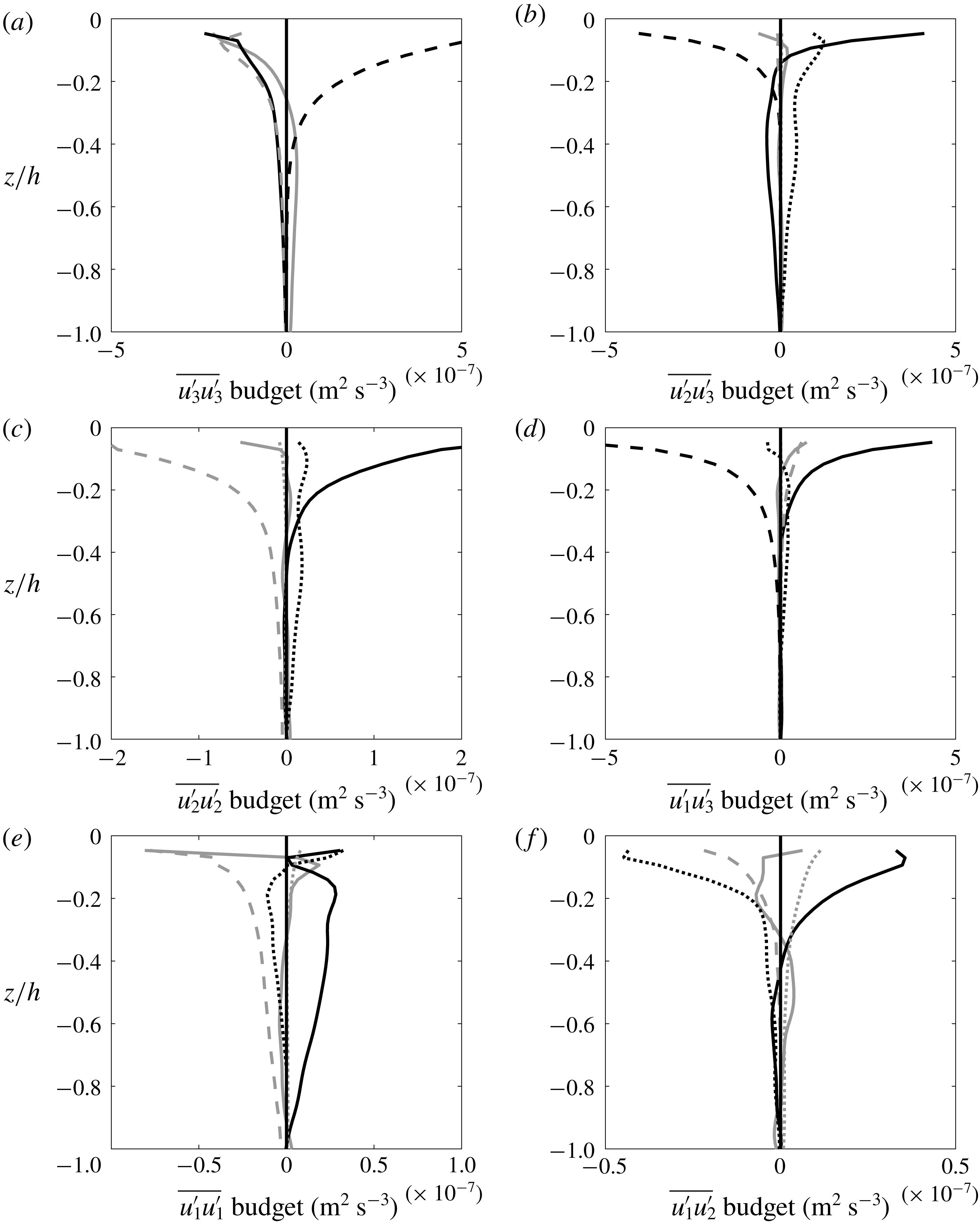
Profiles of terms of the Reynolds stress budgets within the mixed layer. The terms are from the budgets of (a)
 $\overline{u_{3}^{\prime }u_{3}^{\prime }}$
, (b)
 $\overline{u_{2}^{\prime }u_{3}^{\prime }}$
, (c)
 $\overline{u_{2}^{\prime }u_{2}^{\prime }}$
, (d)
 $\overline{u_{1}^{\prime }u_{3}^{\prime }}$
, (e)
 $\overline{u_{1}^{\prime }u_{1}^{\prime }}$
and (f)
 $\overline{u_{1}^{\prime }u_{2}^{\prime }}$
in a flow with
 $La_{t}=0.3$
. Shown are the Stokes production (– –), shear production (
 $\cdots \cdots$
), pressure–strain term (——), stress transport (grey solid), dissipation (grey dashed) and Coriolis term (grey dotted).

Figure 1 shows the terms of the Reynolds stress budgets (2.2) from the LES with
 $La_{t}=0.3$
. In all of the budgets, the pressure–strain term is one of the largest magnitude terms. This demonstrates the need to accurately model
 $\unicode[STIX]{x1D6F1}_{ij}$
for any Langmuir turbulence closure scheme that uses the Reynolds stress budgets, regardless of whether the scheme is derived from these budgets or if it uses these budgets explicitly. The buoyancy and Coriolis terms are too small to plot on these axes (except the Coriolis term in the
 $\overline{u_{1}^{\prime }u_{2}^{\prime }}$
budget). The largest term in the budget for the vertical velocity variance,
 $\overline{u_{3}^{\prime }u_{3}^{\prime }}$
, is Stokes production near the surface, which is balanced by a combination of pressure–strain term (which is decomposed in figure 2
a), stress transport, and dissipation through the LES subgrid scheme. Below 0.5
 $h_{m}$
the stress transport provides the main source of
 $\overline{u_{3}^{\prime }u_{3}^{\prime }}$
, consistent with the transport of energy from near the surface to the rest of the mixed layer through down-welling jets in Langmuir turbulence (McWilliams et al.
Reference McWilliams, Sullivan and Moeng1997; Polton & Belcher Reference Polton and Belcher2007).
The pressure–strain term is the dominant production term near the surface in the
 $\overline{u_{2}^{\prime }u_{2}^{\prime }}$
(cross-wind velocity variance) budget, and away from the surface in the
 $\overline{u_{1}^{\prime }u_{1}^{\prime }}$
(along-wind velocity variance) budget, in both cases being balanced predominantly by dissipation. Shear production of
 $\overline{u_{2}^{\prime }u_{2}^{\prime }}$
is present over the entire mixed layer, while the shear production is a sink of
 $\overline{u_{1}^{\prime }u_{1}^{\prime }}$
away from the surface. The largest terms in the
 $\overline{u_{1}^{\prime }u_{1}^{\prime }}$
budget are an order of magnitude smaller than those of the
 $\overline{u_{3}^{\prime }u_{3}^{\prime }}$
and
 $\overline{u_{2}^{\prime }u_{2}^{\prime }}$
budgets. The dissipation is not evenly distributed across the velocity variance budgets, with the dissipation of
 $\overline{u_{1}^{\prime }u_{1}^{\prime }}$
being smaller than the dissipation of the other velocity variances. Previous studies (Mironov et al.
Reference Mironov, Gryanik, Moeng, Olbers and Warncke2000; Mironov Reference Mironov2001) suggest that the presence of anisotropic dissipation in LES represents unresolved components of the slow pressure–strain term, which is discussed in appendix B.
The budgets for the vertical momentum fluxes,
 $\overline{u_{1}^{\prime }u_{3}^{\prime }}$
and
 $\overline{u_{2}^{\prime }u_{3}^{\prime }}$
, are dominated by a balance between Stokes production and pressure–strain term near the surface. Away from the surface the
 $\overline{u_{2}^{\prime }u_{3}^{\prime }}$
budget is a balance between pressure–strain term and shear production. The terms of the
 $\overline{u_{1}^{\prime }u_{2}^{\prime }}$
budget are an order of magnitude smaller than the other momentum flux budgets, and the pressure–strain term is a significant component of the
 $\overline{u_{1}^{\prime }u_{2}^{\prime }}$
budget over most of the mixed layer. The dissipation of the momentum fluxes is small relative to other terms in their budgets, indicating that the LES is resolving the physical processes that are important in these budgets.
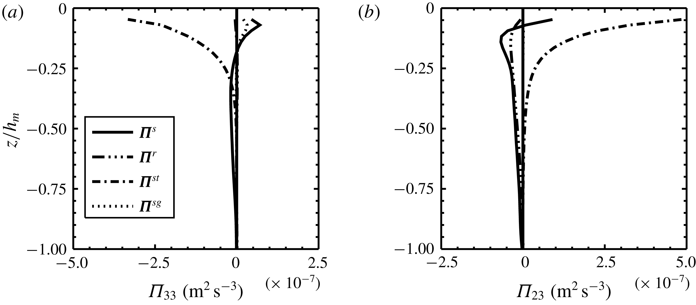
Components of pressure–strain term from the (a)
 $\overline{u_{3}^{\prime }u_{3}^{\prime }}$
and (b)
 $\overline{u_{2}^{\prime }u_{3}^{\prime }}$
budgets in a flow with
 $La_{t}=0.3$
. The components of the pressure–strain term are defined in (2.3), and the buoyancy and Coriolis components are too small to plot on these axes.

To understand which processes contribute to the pressure–strain term, figure 2 shows the components of
 $\unicode[STIX]{x1D6F1}_{33}$
and
 $\unicode[STIX]{x1D6F1}_{23}$
, as defined in (2.3). The largest components of the pressure–strain term are the Stokes, rapid and slow terms, with this trend being observed for all elements of the pressure–strain term tensor (not shown). Near the surface, the Stokes pressure–strain term is the largest component of
 $\unicode[STIX]{x1D6F1}_{33}$
and
 $\unicode[STIX]{x1D6F1}_{23}$
, and it decays with depth, similar to the exponential Stokes drift profile. The rapid and slow components of the pressure–strain term are smaller than the Stokes component near the surface, but become significant components of
 $\unicode[STIX]{x1D72B}$
away from the surface, with
 $\unicode[STIX]{x1D6F1}_{23}^{s}$
and
 $\unicode[STIX]{x1D6F1}_{23}^{r}$
having similar magnitudes while
 $|\unicode[STIX]{x1D6F1}_{33}^{s}|\gg |\unicode[STIX]{x1D6F1}_{33}^{r}|$
. The shapes and magnitudes of
 $\unicode[STIX]{x1D72B}^{st}$
and
 $\unicode[STIX]{x1D72B}^{r}$
are similar to the Stokes and shear production terms of their budgets respectively (figure 1), but the pressure–strain term components have the opposite sign to the production terms. The largest element of the subgrid pressure–strain term is
 $\unicode[STIX]{x1D6F1}_{33}^{sg}$
, which is still an order of magnitude smaller than the largest component of
 $\unicode[STIX]{x1D6F1}_{33}$
at the same depth. This indicates that the pressure fluctuations in the LES represent the dynamics of Langmuir turbulence rather than numerical effects due to unresolved scales.
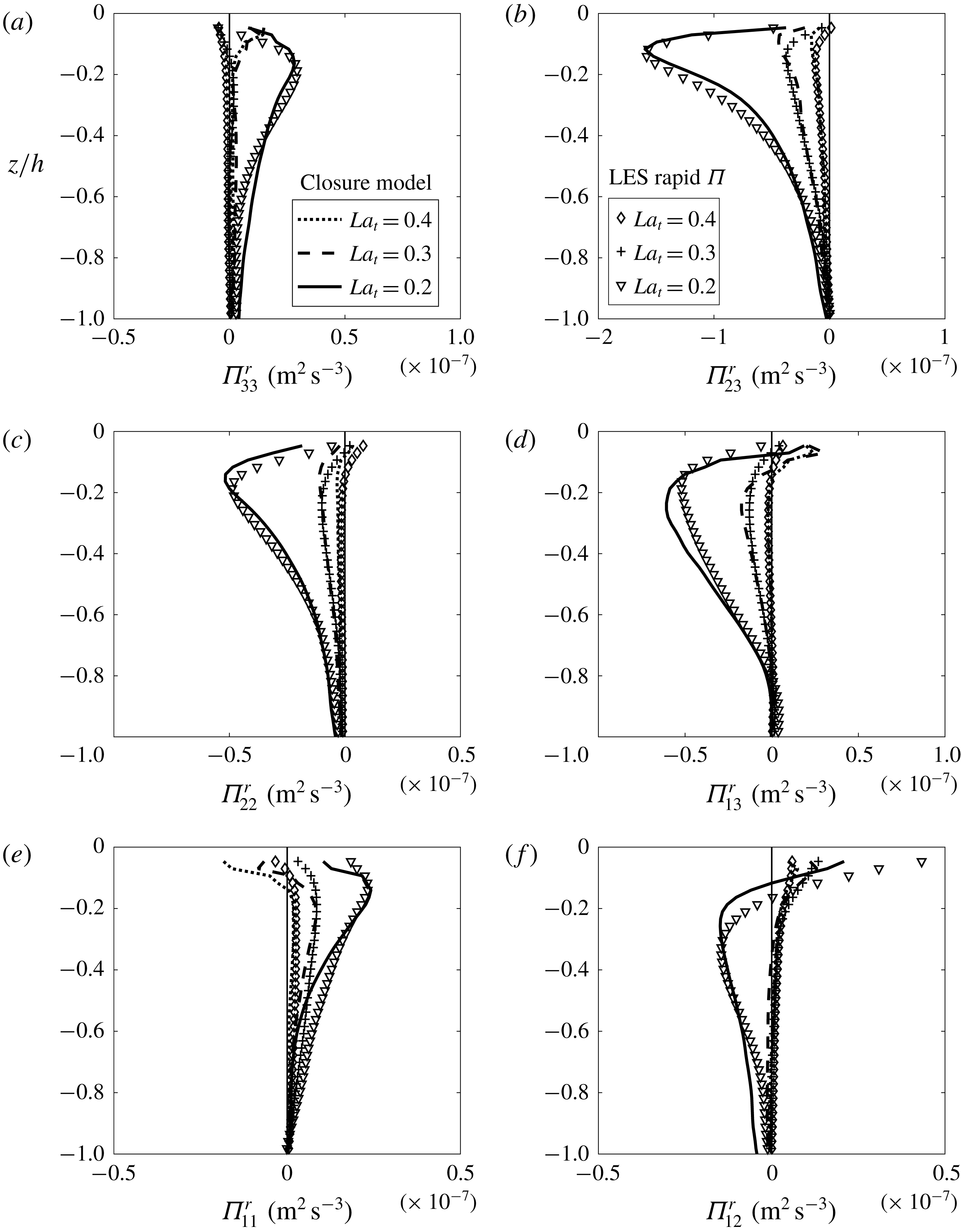
Profiles of the rapid pressure–strain term,
 $\unicode[STIX]{x1D72B}^{r}$
, from LES with varying
 $La_{t}$
. Also shown is the closure model (2.8) using
 $C_{1}=0.6$
,
 $C_{2}=0.3$
and
 $C_{3}=-0.7$
. The elements of the rapid pressure–strain term are (a)
 $\unicode[STIX]{x1D6F1}_{33}^{r}$
, (b)
 $\unicode[STIX]{x1D6F1}_{23}^{r}$
, (c)
 $\unicode[STIX]{x1D6F1}_{22}^{r}$
, (d)
 $\unicode[STIX]{x1D6F1}_{13}^{r}$
, (e)
 $\unicode[STIX]{x1D6F1}_{11}^{r}$
and (f)
 $\unicode[STIX]{x1D6F1}_{12}^{r}$
. Please note the change in horizontal scales between panels.

4.2 Rapid pressure–strain term
Figure 3 shows the LES profiles of the rapid pressure–strain term,
 $\unicode[STIX]{x1D72B}^{r}$
, for a range of
 $La_{t}$
. Also shown is the closure model for
 $\unicode[STIX]{x1D72B}^{r}$
given in (2.8) using
 $C_{1}=0.6$
,
 $C_{2}=0.3$
and
 $C_{3}=-0.7$
, where the Reynolds stresses and current shear have been diagnosed from the LES. The magnitude of all the elements of
 $\unicode[STIX]{x1D72B}^{r}$
increases as
 $La_{t}$
becomes smaller, a property captured by the closure model. A comparison with figure 1 shows that the elements of the rapid pressure–strain term for
 $La_{t}=0.3$
are similar in shape to, opposite in sign to and smaller in magnitude than the explicit shear production within their respective budgets.
The rapid pressure–strain term conserves kinetic energy because it is traceless, a property shared with all components of the pressure–strain term. The rapid pressure–strain term transfers energy from
 $\overline{u_{2}^{\prime }u_{2}^{\prime }}$
to
 $\overline{u_{1}^{\prime }u_{1}^{\prime }}$
in all simulations and, for
 $La_{t}=0.2$
, it also transfers energy from
 $\overline{u_{2}^{\prime }u_{2}^{\prime }}$
to
 $\overline{u_{3}^{\prime }u_{3}^{\prime }}$
, with the closure model capturing the magnitude and shape of both these transfer rates. In the closure model, the appearance of
 $\overline{u_{2}^{\prime }u_{2}^{\prime }}$
to
 $\overline{u_{3}^{\prime }u_{3}^{\prime }}$
transfer at low
 $La_{t}$
results from an increase in the shear production of cross-wind TKE (
 $-\overline{u_{2}^{\prime }u_{3}^{\prime }}\unicode[STIX]{x2202}U_{2}/\unicode[STIX]{x2202}x_{3}$
). This is consistent with Grant & Belcher (Reference Grant and Belcher2009) who showed that while
 $|\overline{u_{2}^{\prime }u_{3}^{\prime }}|$
is zero at the surface, its gradient, and therefore the maximum magnitude of
 $|\overline{u_{2}^{\prime }u_{3}^{\prime }}|$
, increases as
 $La_{t}^{-2}$
. For
 $La_{t}=0.2$
the closure model overestimates the transfer of
 $\overline{u_{2}^{\prime }u_{2}^{\prime }}$
to
 $\overline{u_{3}^{\prime }u_{3}^{\prime }}$
over the lower half of the mixed layer, but this is balanced by an underestimation of the transfer of
 $\overline{u_{2}^{\prime }u_{2}^{\prime }}$
to
 $\overline{u_{1}^{\prime }u_{1}^{\prime }}$
. In the momentum flux budgets the rapid pressure–strain term is negative over most of the mixed layer. As
 $La_{t}$
becomes smaller the off-diagonal elements of
 $\unicode[STIX]{x1D72B}^{r}$
increase in magnitude and the profiles of
 $\unicode[STIX]{x1D6F1}_{23}$
and
 $\unicode[STIX]{x1D6F1}_{12}$
develop negative peaks near the surface. The closure model captures both of these properties of the profiles and shows good agreement with the peak magnitude of all the profiles. These results suggest that the closure model for the rapid pressure–strain term given in (2.8) is appropriate for Langmuir turbulence, despite the turbulence not being primarily driven through rapid distortion by current shear.
4.3 Stokes pressure–strain term
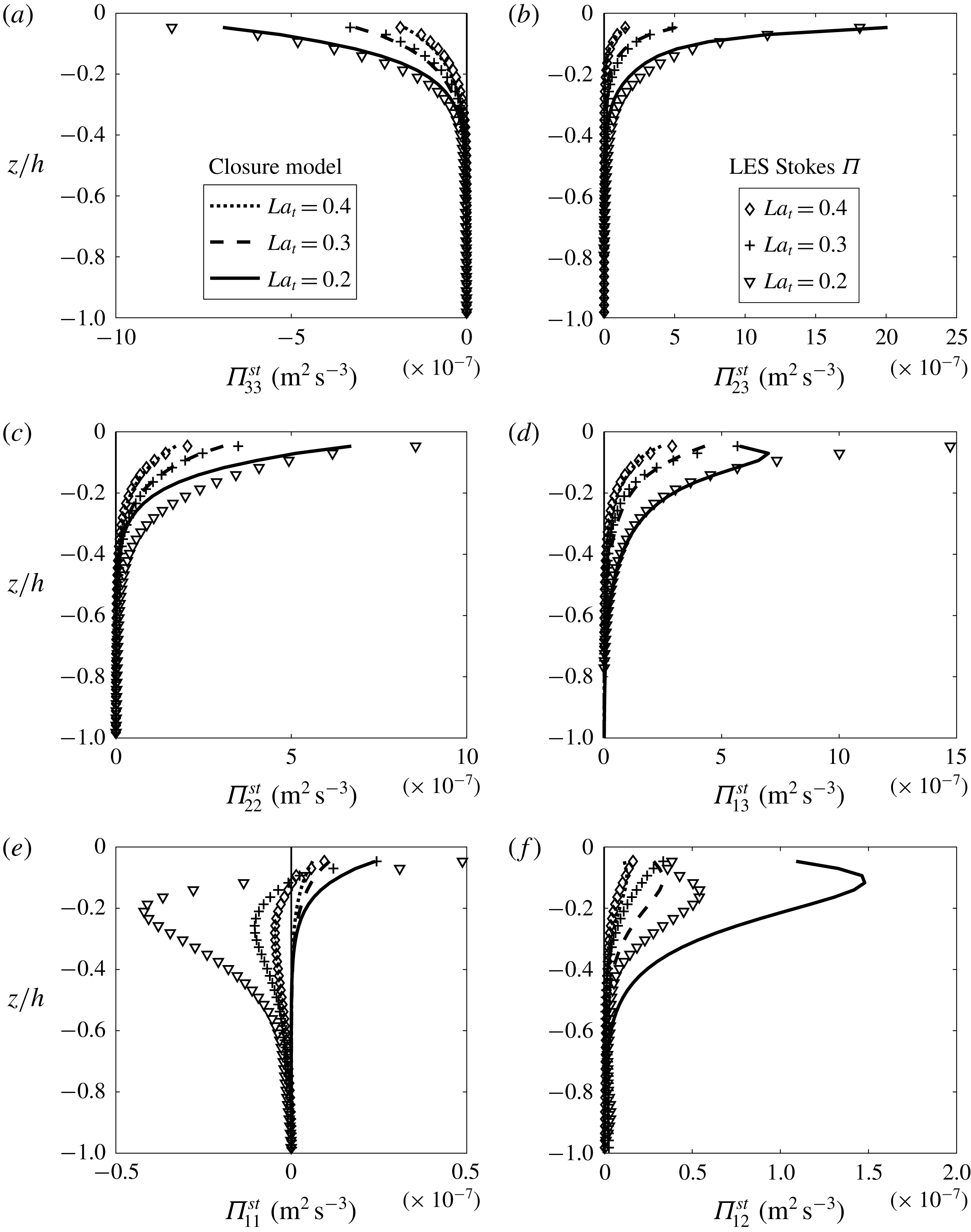
Figure 4 shows the LES profiles of the Stokes pressure–strain term,
 $\unicode[STIX]{x1D72B}^{st}$
, for a range of
 $La_{t}$
. Also shown is the closure model for
 $\unicode[STIX]{x1D72B}^{st}$
given in (2.12) using
 $C_{1}^{st}=1.1$
,
 $C_{2}^{st}=1.4$
and
 $C_{3}^{st}=0.5$
. The Stokes pressure–strain term is the largest component of the pressure–strain term in many of the Reynolds stress budgets (figure 2). Both
 $\unicode[STIX]{x1D6F1}_{11}^{st}$
and
 $\unicode[STIX]{x1D6F1}_{12}^{st}$
are an order of magnitude smaller than the other elements of
 $\unicode[STIX]{x1D72B}^{st}$
. The largest elements of
 $\unicode[STIX]{x1D6F1}_{ij}^{st}$
are concentrated near the surface and are captured reasonably well by the closure model of (2.12) for all
 $La_{t}$
. The closure model is not able to capture
 $\unicode[STIX]{x1D6F1}_{11}^{st}$
, and predicts the correct profile shape for
 $\unicode[STIX]{x1D6F1}_{12}^{st}$
but overestimates its magnitude for all
 $La_{t}$
.
More specifically, in the LES the Stokes drift produces
 $\overline{u_{3}^{\prime }u_{3}^{\prime }}$
(figure 1
a) and the Stokes pressure–strain term transfers energy from
 $\overline{u_{3}^{\prime }u_{3}^{\prime }}$
to
 $\overline{u_{2}^{\prime }u_{2}^{\prime }}$
(figure 4
a,c). This is consistent with Langmuir circulations, near-surface counter-rotating vortices aligned with the wind (Craik & Leibovich Reference Craik and Leibovich1976; Roekel et al.
Reference Roekel, Fox-Kemper, Sullivan, Hamlington and Haney2012), being produced by a mixture of Stokes production and Stokes pressure–strain terms. In LES, an additional transfer of energy to
 $\overline{u_{1}^{\prime }u_{1}^{\prime }}$
deeper in the mixed layer becomes apparent at
 $La_{t}=0.2$
.
Profiles of the Stokes pressure–strain term,
 $\unicode[STIX]{x1D72B}^{st}$
, from LES with varying
 $La_{t}$
. Also shown is the closure model of (2.12) using
 $C_{1}^{st}=1.1$
,
 $C_{2}^{st}=1.4$
and
 $C_{3}^{st}=0.5$
. The elements of the Stokes pressure–strain term are (a)
 $\unicode[STIX]{x1D6F1}_{33}^{st}$
, (b)
 $\unicode[STIX]{x1D6F1}_{23}^{st}$
, (c)
 $\unicode[STIX]{x1D6F1}_{22}^{st}$
, (d)
 $\unicode[STIX]{x1D6F1}_{13}^{st}$
, (e)
 $\unicode[STIX]{x1D6F1}_{11}^{st}$
and (f)
 $\unicode[STIX]{x1D6F1}_{12}^{st}$
. Please note the change in horizontal scales between panels.

Insight into the behaviour of the Stokes closure model can be gained by looking at its components. In the present simulations the closure model for Stokes pressure–strain terms (2.12) becomes,
 $$\begin{eqnarray}\unicode[STIX]{x1D72B}^{st}=\left[\begin{array}{@{}ccc@{}}\left({\displaystyle \frac{C_{2}^{st}-3C_{3}^{st}}{3}}\right)\overline{u_{1}^{\prime }u_{3}^{\prime }}{\displaystyle \frac{\unicode[STIX]{x2202}u_{1}^{st}}{\unicode[STIX]{x2202}x_{3}}} & \left({\displaystyle \frac{C_{2}^{st}-C_{3}^{st}}{2}}\right)\overline{u_{2}^{\prime }u_{3}^{\prime }}{\displaystyle \frac{\unicode[STIX]{x2202}u_{1}^{st}}{\unicode[STIX]{x2202}x_{3}}} & \begin{array}{@{}c@{}}\left[{\displaystyle \frac{C_{1}^{st}}{2}}e+\left({\displaystyle \frac{C_{2}^{st}+C_{3}^{st}}{2}}\right)\unicode[STIX]{x1D622}_{11}\right.\\ ~~\left.+\left({\displaystyle \frac{C_{2}^{st}-C_{3}^{st}}{2}}\right)\unicode[STIX]{x1D622}_{33}\right]{\displaystyle \frac{\unicode[STIX]{x2202}u_{1}^{st}}{\unicode[STIX]{x2202}x_{3}}}\end{array}\\ \left({\displaystyle \frac{C_{2}^{st}-C_{3}^{st}}{2}}\right)\overline{u_{2}^{\prime }u_{3}^{\prime }}{\displaystyle \frac{\unicode[STIX]{x2202}u_{1}^{st}}{\unicode[STIX]{x2202}x_{3}}} & -{\displaystyle \frac{2}{3}}C_{2}^{st}\overline{u_{1}^{\prime }u_{3}^{\prime }}{\displaystyle \frac{\unicode[STIX]{x2202}u_{1}^{st}}{\unicode[STIX]{x2202}x_{3}}} & \left({\displaystyle \frac{C_{2}^{st}+C_{3}^{st}}{2}}\right)\overline{u_{1}^{\prime }u_{2}^{\prime }}{\displaystyle \frac{\unicode[STIX]{x2202}u_{1}^{st}}{\unicode[STIX]{x2202}x_{3}}}\\ \begin{array}{@{}c@{}}\left[{\displaystyle \frac{C_{1}^{st}}{2}}e+\left({\displaystyle \frac{C_{2}^{st}+C_{3}^{st}}{2}}\right)\unicode[STIX]{x1D622}_{11}\right.\\ ~~\left.+\left({\displaystyle \frac{C_{2}^{st}-C_{3}^{st}}{2}}\right)\unicode[STIX]{x1D622}_{33}\right]{\displaystyle \frac{\unicode[STIX]{x2202}u_{1}^{st}}{\unicode[STIX]{x2202}x_{3}}}\end{array} & \left({\displaystyle \frac{C_{2}^{st}+C_{3}^{st}}{2}}\right)\overline{u_{1}^{\prime }u_{2}^{\prime }}{\displaystyle \frac{\unicode[STIX]{x2202}u_{1}^{st}}{\unicode[STIX]{x2202}x_{3}}} & \left({\displaystyle \frac{C_{2}^{st}+3C_{3}^{st}}{3}}\right)\overline{u_{1}^{\prime }u_{3}^{\prime }}{\displaystyle \frac{\unicode[STIX]{x2202}u_{1}^{st}}{\unicode[STIX]{x2202}x_{3}}}\end{array}\right].\end{eqnarray}$$
The diagonal elements of the model (4.1) are proportional to the Stokes production of TKE,
 $-\overline{u_{1}^{\prime }u_{3}^{\prime }}\left(\unicode[STIX]{x2202}u_{1}^{st}/\unicode[STIX]{x2202}x_{3}\right)$
. This means that, like the Stokes production (figure 1), the model’s energy transfer between velocity components is maximum near the surface. This is an accurate model for
 $\unicode[STIX]{x1D6F1}_{22}^{st}$
and
 $\unicode[STIX]{x1D6F1}_{33}^{st}$
across a range of
 $La_{t}$
, transferring TKE from
 $\overline{u_{3}^{\prime }u_{3}^{\prime }}$
to
 $\overline{u_{2}^{\prime }u_{2}^{\prime }}$
at approximately half the rate at which
 $\overline{u_{3}^{\prime }u_{3}^{\prime }}$
is produced by Stokes production, but it is unable to capture
 $\unicode[STIX]{x1D6F1}_{11}^{st}$
because its LES profile has a sub-surface peak that is most apparent for
 $La_{t}=0.2$
. To compensate and remain traceless, the closure model underestimates the production of
 $\overline{u_{2}^{\prime }u_{2}^{\prime }}$
by
 $\unicode[STIX]{x1D6F1}_{22}^{st}$
away from the surface for
 $La_{t}=0.2$
. Physical intuition into the model can be gained by looking at the diagonal elements of (4.1) and (2.12), which show that the Stokes drift strain (
 $C_{2}^{st}$
term) converts equal amounts of along-wind and vertical TKE into the cross-wind direction, while the Stokes rotation rate (
 $C_{3}^{st}$
term) converts vertical TKE into the along-wind direction. The coefficients are such that the latter conversion rate almost balances the former in the along-wind TKE budget, consistent with LES where the maximum of
 $\unicode[STIX]{x1D6F1}_{11}^{st}$
is an order of magnitude smaller than
 $\unicode[STIX]{x1D6F1}_{22}^{st}$
and
 $\unicode[STIX]{x1D6F1}_{33}^{st}$
.
The largest off-diagonal components of
 $\unicode[STIX]{x1D72B}^{st}$
in LES are
 $\unicode[STIX]{x1D6F1}_{23}^{st}$
and
 $\unicode[STIX]{x1D6F1}_{13}^{st}$
, which are comparable and opposite in magnitude to the Stokes production terms in their respective flux budgets (figure 1). The closure model is able to capture these two components across a range of
 $La_{t}$
. In fact the
 $\unicode[STIX]{x1D6F1}_{23}^{st}$
is proportional to the Stokes production term of its budget, while the
 $\unicode[STIX]{x1D6F1}_{13}^{st}$
is more complex (4.1). The closure model also agrees with the shape of
 $\unicode[STIX]{x1D6F1}_{12}^{st}$
from the LES, but it overestimates its magnitude. Notably, while the diagonal components of the closure model are maximum at the surface, the off-diagonal components can peak within the mixed layer because of the presence of Reynolds stresses which tend to zero at the surface (
 $\overline{u_{3}^{\prime }u_{3}^{\prime }}$
and
 $\overline{u_{2}^{\prime }u_{3}^{\prime }}$
), counteracting the surface maximum of
 $\unicode[STIX]{x2202}u_{1}^{st}/\unicode[STIX]{x2202}x_{3}$
.
The good agreement between LES profiles and the closure model of (2.12) for the largest elements of the Stokes pressure–strain term,
 $\unicode[STIX]{x1D72B}^{st}$
, is one of the key results of this paper. The Stokes pressure–strain term is one of the largest terms in the Reynolds stress budgets, and effectively cancels out a significant fraction of many of the explicit Stokes production terms in (2.2), and the implications of these results will be discussed in more detail in § 5. While the closure model captures many of the largest
 $\unicode[STIX]{x1D72B}^{st}$
effects, the closure model does not agree with the LES for smaller pressure terms such as
 $\unicode[STIX]{x1D6F1}_{11}^{st}$
,
 $\unicode[STIX]{x1D6F1}_{12}^{st}$
and, away from the surface,
 $\unicode[STIX]{x1D6F1}_{22}^{st}$
. These differences could arise from simplifications made in deriving (2.12), such as neglecting curvature of the Stokes drift profile and assuming a single-point closure.
Profiles of the slow pressure–strain terms, (a)
 $\unicode[STIX]{x1D6F1}_{23}^{s}$
and (b)
 $\unicode[STIX]{x1D6F1}_{13}^{s}$
, from LES. Also shown is the Rotta (return-to-isotropy) closure model (2.7) using
 $C_{0}=0.2$
.

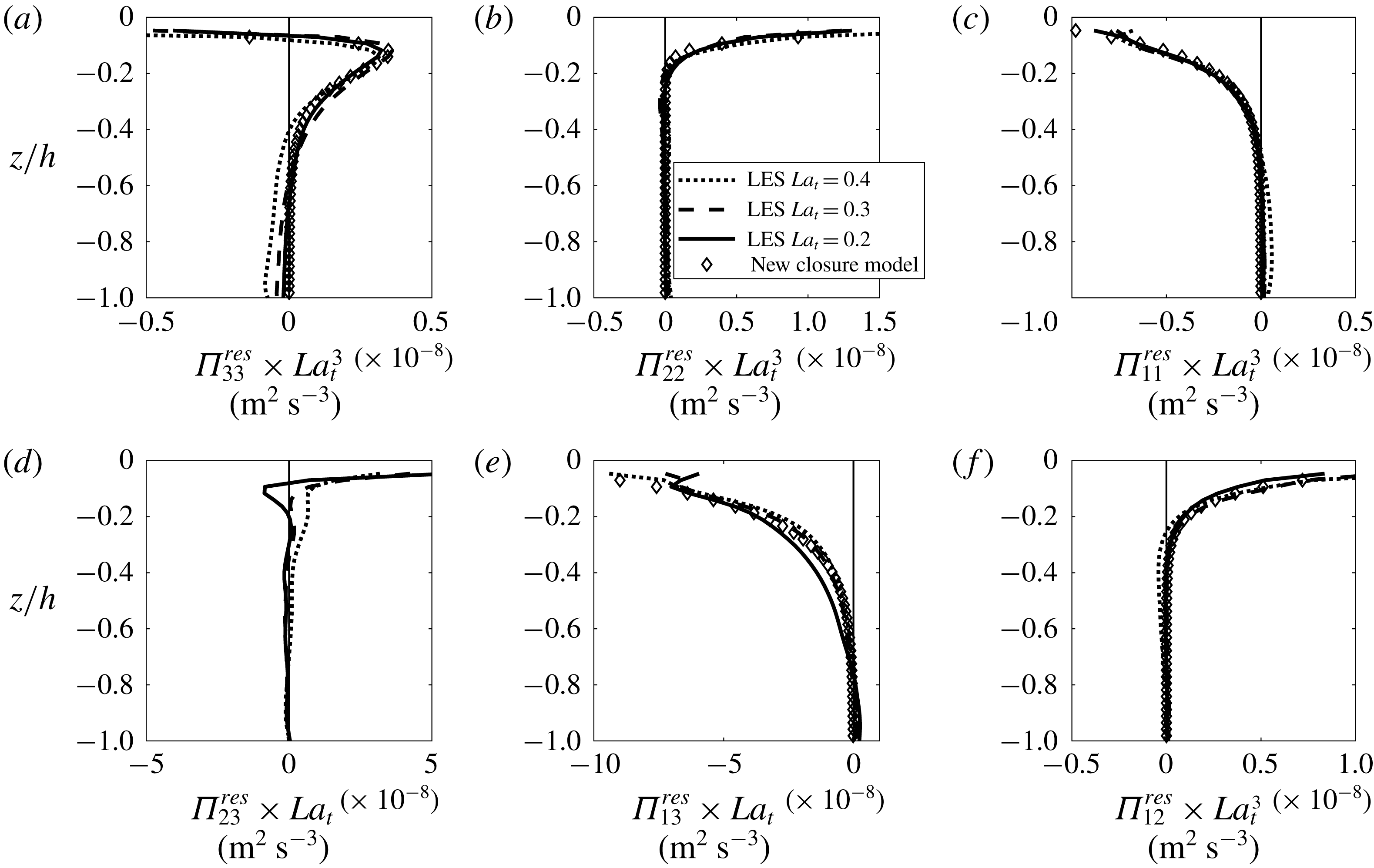
Profiles of the residual pressure–strain terms,
 $\unicode[STIX]{x1D6F1}_{ij}^{res}$
, from LES over a range of
 $La_{t}$
. The residual terms are calculated from (4.2) using
 $C_{0}=0.2$
. Diamonds show the new closure model,
 $F_{ij}(La_{t},z/\unicode[STIX]{x1D6FF})$
, using the parameter values listed in the text. The profiles have been scaled by a function of
 $La_{t}^{n}$
to demonstrate their collapse across simulations. Note that
 $n=1$
for
 $\unicode[STIX]{x1D6F1}_{13}^{res}$
and
 $\unicode[STIX]{x1D6F1}_{23}^{res}$
, and
 $n=3$
for all other profiles. Please note the change in horizontal scales between panels.

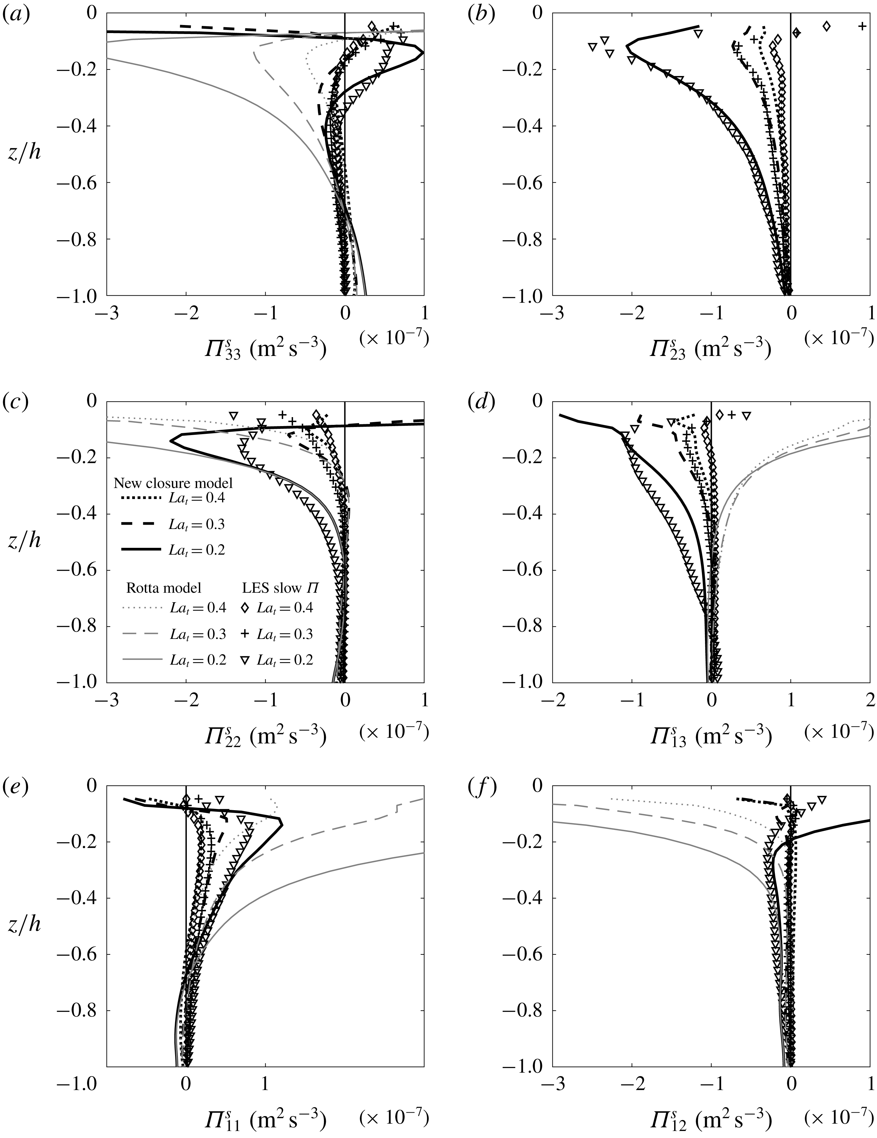
Comparison of the slow pressure–strain components,
 $\unicode[STIX]{x1D6F1}_{ij}^{s}$
, from LES (symbols) and the new closure model proposed in (4.2) (black lines). Also shown are the Rotta closure model prediction for each profile (thin grey lines). The closure parameters are given in the text.

4.4 Slow pressure–strain term
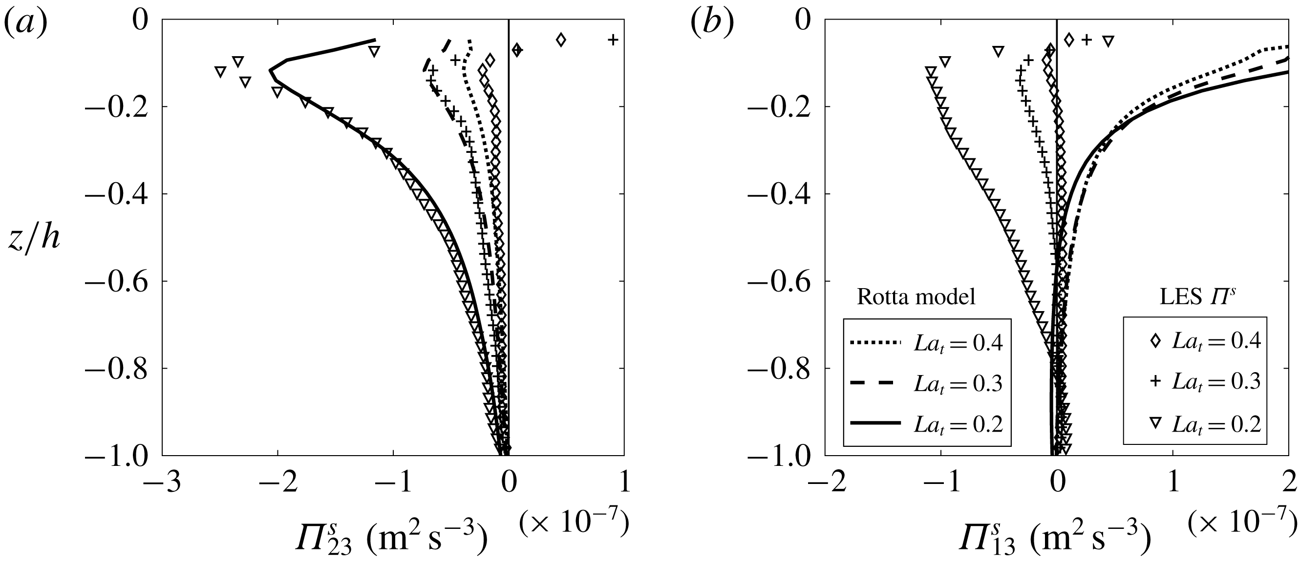
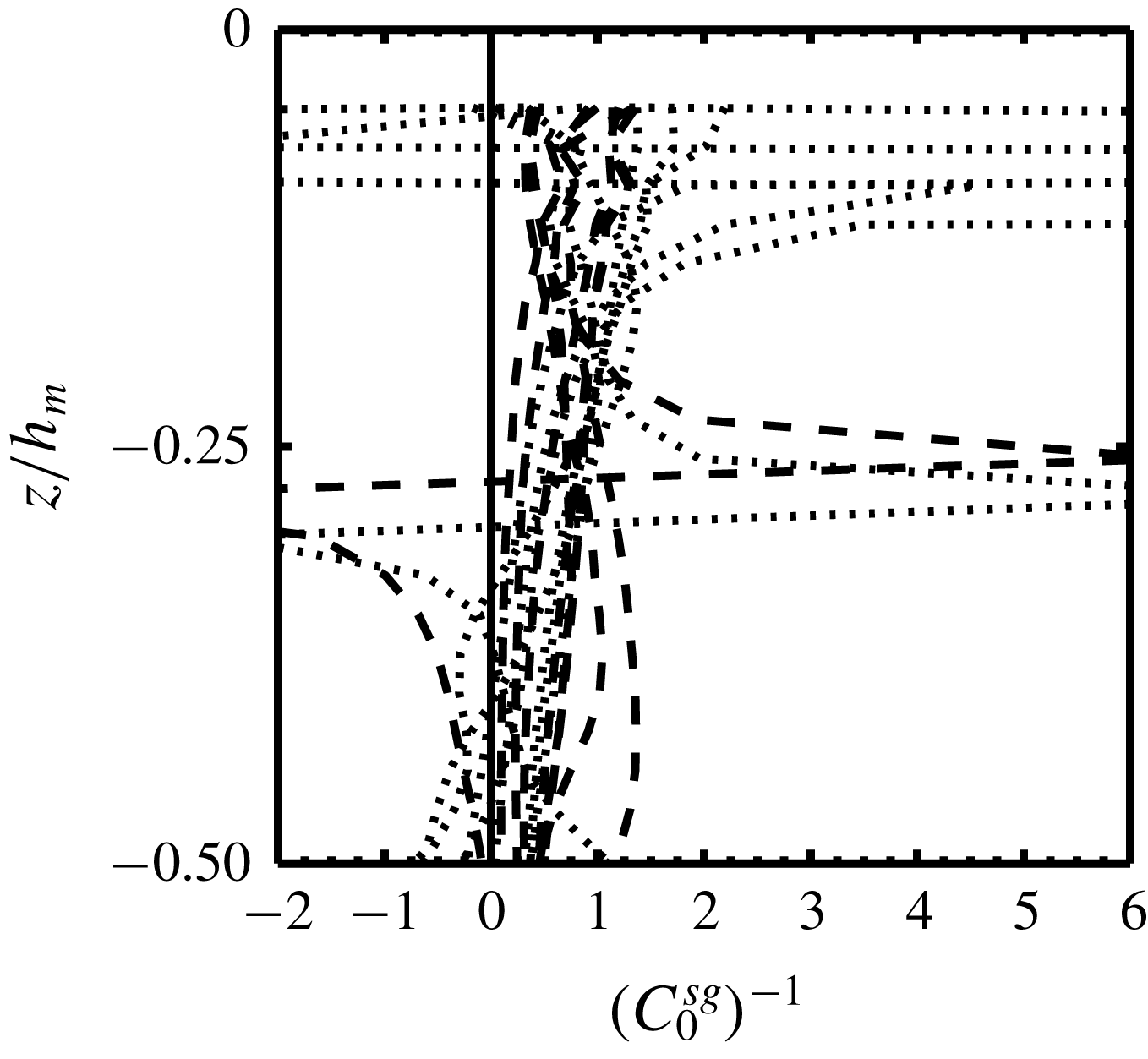
Figure 5 shows LES profiles of two components of the slow pressure–strain term. Also shown is the Rotta (or return-to-isotropy) closure model given by (2.7) using
 $C_{0}=0.2$
. The Rotta model shows good agreement with the LES profiles of
 $\unicode[STIX]{x1D6F1}_{23}^{s}$
over the depth of the mixed layer and their variation with
 $La_{t}$
. However, there are large differences between the Rotta model and the LES profiles of
 $\unicode[STIX]{x1D6F1}_{13}^{s}$
, in fact
 $\unicode[STIX]{x1D6F1}_{13}^{s}$
is increasing the anisotropy for small
 $La_{t}$
. The Rotta model also does not accurately reproduce the other four
 $\unicode[STIX]{x1D6F1}_{ij}^{s}$
components (shown later in figure 7). Based on the agreement between the Rotta model and
 $\unicode[STIX]{x1D6F1}_{23}$
, we propose a simple extension to the Rotta model,
 $$\begin{eqnarray}\unicode[STIX]{x1D6F1}_{ij}^{s}=-\frac{\unicode[STIX]{x1D622}_{ij}}{C_{0}\unicode[STIX]{x1D70F}_{\unicode[STIX]{x1D700}}}e+\unicode[STIX]{x1D6F1}_{ij}^{res}\approx -\frac{\unicode[STIX]{x1D622}_{ij}}{C_{0}\unicode[STIX]{x1D70F}_{\unicode[STIX]{x1D700}}}e+F_{ij}(La_{t},z/\unicode[STIX]{x1D6FF}),\end{eqnarray}$$
where
 $F_{ij}(La_{t},z/\unicode[STIX]{x1D6FF})$
is a closure model for the residual term (
 $\unicode[STIX]{x1D6F1}_{ij}^{res}$
) of the slow pressure–strain that does not follow the Rotta model, and we shall assume that it is a function of the Langmuir number
 $La_{t}$
, and a non-dimensional depth (nominally
 $z/\unicode[STIX]{x1D6FF}$
here). Figure 6 shows
 $\unicode[STIX]{x1D6F1}_{ij}^{res}$
, calculated from (4.2), assuming that
 $C_{0}=0.2$
as implied by the agreement between the Rotta model and
 $\unicode[STIX]{x1D6F1}_{23}^{s}$
. The profiles of
 $\unicode[STIX]{x1D6F1}_{ij}^{res}$
collapse across the simulations once they have been scaled by
 $La_{t}^{n}$
where
 $n$
varies between components. Several of the collapsed profiles decay exponentially with depth and are concentrated near the surface, suggesting that the appropriate non-dimensional depth may be
 $z/\unicode[STIX]{x1D6FF}$
where
 $\unicode[STIX]{x1D6FF}$
is the Stokes decay depth. This leads us to propose the following simple closure model for these components of
 $\unicode[STIX]{x1D72B}^{res}$
,
 $$\begin{eqnarray}F_{ij}=A_{0}La_{t}^{n}e^{A_{1}z/\unicode[STIX]{x1D6FF}},\end{eqnarray}$$
where
 $A_{0}$
,
 $n$
and
 $A_{1}$
are constants (but can depend on
 $i$
and
 $j$
). The profiles of
 $\unicode[STIX]{x1D6F1}_{33}^{res}$
and
 $\unicode[STIX]{x1D6F1}_{23}^{res}$
do not follow a simple exponential decay, so we diagnose the former by making
 $\unicode[STIX]{x1D6F1}_{ij}^{res}$
traceless (
 $\unicode[STIX]{x1D6F1}_{33}^{res}=-\unicode[STIX]{x1D6F1}_{11}^{res}-\unicode[STIX]{x1D6F1}_{22}^{res}$
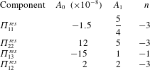
), and the latter is assumed to be zero due to the good agreement between the Rotta model and LES for this component (figure 5a). This closure model (symbols in figure 6) agrees well with the
 $\unicode[STIX]{x1D6F1}_{ij}^{res}$
profiles from LES. The closure parameters are shown in table 1. Note that the closure model proposed here for the residual term is empirical, and it does not obey tensor transformation and symmetry constraints (in contrast to the rapid, Stokes, and Rotta closure models presented earlier). As a result, it should only presently be applied in co-ordinates aligned with the Stokes drift/wind direction.
Closure model parameters for the residual component of the slow pressure–strain term,
 $\unicode[STIX]{x1D72B}^{res}\approx A_{0}La_{t}^{-n}\exp (A_{1}z/\unicode[STIX]{x1D6FF})$
.

Figure 7 shows the LES profiles of slow pressure–strain along with the new closure model proposed in the above paragraph (4.2). The new closure model shows good agreement with the LES profiles, this is due mainly to the new residual closure term, as can be seen by the poor agreement between the Rotta model (thin grey lines) and the LES profiles (symbols). The improvement provided by the new closure model is particularly noticeable for
 $\unicode[STIX]{x1D6F1}_{13}^{s}$
,
 $\unicode[STIX]{x1D6F1}_{11}^{s}$
, and
 $\unicode[STIX]{x1D6F1}_{12}^{s}$
, but for
 $\unicode[STIX]{x1D6F1}_{22}^{s}$
and
 $\unicode[STIX]{x1D6F1}_{33}^{s}$
it still reduces the error compared to the Rotta model alone.
While the new closure model for
 $\unicode[STIX]{x1D72B}^{res}$
is empirical, there must be a physical mechanism that produces
 $\unicode[STIX]{x1D72B}^{res}$
. This will be discussed further in § 5, but for now we note two interesting points. First, the
 $La_{t}$
scaling of
 $\unicode[STIX]{x1D72B}^{res}$
components (figure 6) is not the same as the scaling for the kinetic energy budgets (
 $u_{\ast }^{3}La_{t}^{-2}/h_{m}$
, Grant & Belcher Reference Grant and Belcher2009) or momentum flux budgets (
 $u_{\ast }^{3}La_{t}^{-2/3}/h_{m}$
). Second, the Rotta model has previously been shown to be accurate for shear-driven turbulence (Andren & Moeng Reference Andren and Moeng1993). It is interesting that in Langmuir turbulence the Rotta model only accurately captures
 $\unicode[STIX]{x1D6F1}_{23}^{s}$
, since
 $\overline{u_{2}^{\prime }u_{3}^{\prime }}$
is the only component of the Reynolds stress where mean shear production is the dominant term sustaining anisotropy over most of the mixed layer (figure 1). The other Reynolds stress components are predominantly sustained by pressure–strain or Stokes terms. Note that here ‘sustaining’ terms are those that drive the Reynolds stress component away from isotropy, and that
 $\unicode[STIX]{x1D622}_{23}$
,
 $\unicode[STIX]{x1D622}_{22}$
,
 $\unicode[STIX]{x1D622}_{33}$
and
 $\unicode[STIX]{x1D622}_{12}$
are positive while
 $\unicode[STIX]{x1D622}_{13}$
and
 $\unicode[STIX]{x1D622}_{11}$
are negative, as seen from the Rotta models in figure 7.
5 Discussion
5.1 Direct effect of Stokes drift on pressure–strain terms (
 $\unicode[STIX]{x1D72B}^{st}$
)

The presence of a Stokes drift induces turbulent pressure fluctuations, resulting in a new pressure–strain term,
 $\unicode[STIX]{x1D72B}^{st}$
. In the present paper
 $\unicode[STIX]{x1D72B}^{st}$
has been shown to be comparable, and opposite in magnitude, to many explicit Stokes drift terms in the Reynolds stress budgets. This demonstrates that closure schemes which include Stokes drift terms in the budgets of Reynolds stresses or TKE (i.e. D’Alessio et al.
Reference D’Alessio, Abdella and McFarlane1998; Kantha & Clayson Reference Kantha and Clayson2004), should always include a closure model for Stokes drift effects in the pressure–strain term. While the total TKE is not directly affected by
 $\unicode[STIX]{x1D72B}^{st}$
, neglecting to consider
 $\unicode[STIX]{x1D72B}^{st}$
will limit the ability of closure schemes to predict the partitioning of TKE between velocity components in Langmuir turbulence, which is necessary to quantify directional (i.e. vertical) turbulent mixing and the Eulerian currents induced by Stokes drift (Pearson Reference Pearson2018). Neglecting
 $\unicode[STIX]{x1D72B}^{st}$
will also limit the ability of closure schemes to anticipate off-diagonal Reynolds stresses (turbulent fluxes), which are essential to predict because it is the divergence of these fluxes that quantify the effects of turbulence on mean flow. In § 5.4 we outline how these new
 $\unicode[STIX]{x1D72B}$
closure models could be implemented in first- and second-order closure schemes. Harcourt (Reference Harcourt2013) demonstrated some of the effects that differing pressure–strain correlation closure models could have on the predictions made by turbulence closure schemes.
In the present paper a new closure model for
 $\unicode[STIX]{x1D72B}^{st}$
has been presented which agrees with
 $\unicode[STIX]{x1D72B}^{st}$
profiles diagnosed from LES. This model depends on the local Reynolds stresses and the local Stokes drift gradient, it was derived from the dynamics of pressure fluctuations, and it shares similarities with the model for Eulerian shear-induced pressure–strain terms (
 $\unicode[STIX]{x1D72B}^{r}$
). However, the coefficients of Stokes shear terms in the
 $\unicode[STIX]{x1D72B}^{st}$
closure model (2.12) are different from the coefficients of Eulerian shear terms in the
 $\unicode[STIX]{x1D72B}^{r}$
model (2.8). This result, coupled with the different respective forms of the Stokes and shear production terms in the Reynolds stress budgets (2.2), suggests that simply replacing Eulerian shear by Lagrangian shear in existing turbulence closure schemes (D’Alessio et al.
Reference D’Alessio, Abdella and McFarlane1998; Kantha & Clayson Reference Kantha and Clayson2004) and
 $\unicode[STIX]{x1D72B}$
closure models (H13) is not sufficient to account for the effects of Langmuir turbulence. This result could also explain why first-order closure schemes for Langmuir turbulence that diffuse momentum along Lagrangian, rather than Eulerian, velocity gradients result in complex profiles of eddy diffusivity when fitted to results from LES (McWilliams et al.
Reference McWilliams, Huckle, Liang and Sullivan2012, Reference McWilliams, Huckle, Liang and Sullivan2014). Prior to the new
 $\unicode[STIX]{x1D72B}^{st}$
model, only two studies (Harcourt Reference Harcourt2013, Reference Harcourt2015, H13 and H15 respectively) have included Stokes drift effects in a closure model for
 $\unicode[STIX]{x1D72B}$
, and we shall discuss these in comparison to the new model in § 5.3.
5.2 Indirect effects of Stokes drift (
$\unicode[STIX]{x1D72B}^{r}$
and
$\unicode[STIX]{x1D72B}^{s}$
)


The Stokes drift also changes the rapid and slow pressure–strain terms (
 $\unicode[STIX]{x1D72B}^{r}$
and
 $\unicode[STIX]{x1D72B}^{s}$
), which led us to develop new closure models for these terms in Langmuir turbulence. The rapid pressure–strain term
 $\unicode[STIX]{x1D72B}^{r}$
in Langmuir turbulence can be modelled using the same functional form as existing
 $\unicode[STIX]{x1D72B}^{r}$
models, but with non-dimensional coefficients that differ from existing models. The Stokes drift has a more significant effect on the slow pressure–strain term,
 $\unicode[STIX]{x1D72B}^{s}$
. In Langmuir turbulence the classic Rotta model is a poor closure model for five out of six components of
 $\unicode[STIX]{x1D72B}^{s}$
. The Rotta model was originally developed for idealized turbulence driven by mean shear, and the presence of an alternative forcing (wave-driven Stokes drift) may be the reason the Rotta model is not sufficient in Langmuir turbulence. This hypothesis is supported by both our LES results, where the one component of
 $\unicode[STIX]{x1D72B}^{s}$
that follows the Rotta model is also the only component of anisotropy that is sustained by mean shear, and by previous LES studies of flows dominated by mechanisms other than mean shear, which have shown that the Rotta model is inaccurate for
 $\unicode[STIX]{x1D72B}^{s}$
in strong convection (Ding et al.
Reference Ding, Nguyen, Liu, Otte and Tong2018), and for the pressure-scalar co-variances in rotating convection (Mironov Reference Mironov2001). Following this idea, we have demonstrated a closure model for the non-Rotta part of
 $\unicode[STIX]{x1D72B}^{s}$
that is empirical and based on non-dimensional parameters. Future work should attempt to find a
 $\unicode[STIX]{x1D72B}^{s}$
closure model for Langmuir turbulence that is physically based, like the models presented for
 $\unicode[STIX]{x1D72B}^{r}$
and
 $\unicode[STIX]{x1D72B}^{st}$
. An example of this approach, for turbulent flows with buoyancy, is the recent work of Bou-Zeid et al. (Reference Bou-Zeid, Gao, Ansorge and Katul2018) which developed a closure model for
 $\unicode[STIX]{x1D72B}$
that was a function of the Richardson number in addition to the Rotta model.
In addition to the Rotta model, there are several other more complex closure models for
 $\unicode[STIX]{x1D72B}^{s}$
, and they can broadly be separated into nonlinear return-to-isotropy models and near-wall models (Pope Reference Pope2001). However like the Rotta model neither of these closure models can capture the behaviour of
 $\unicode[STIX]{x1D72B}^{s}$
seen in Langmuir turbulence (figure 7). Wall models represent the inhibition of wall-normal velocity when close to the wall, typically by redistributing
 $\overline{u_{3}^{\prime }u_{3}^{\prime }}$
into horizontal velocity components (Daly & Harlow Reference Daly and Harlow1970; Pope Reference Pope2001, H15), while figure 7 shows that
 $\unicode[STIX]{x1D72B}^{s}$
, and its biases relative to the Rotta model, are opposite in sign for each of the horizontal TKE components. In contrast, nonlinear return-to-isotropy models can account for observations that anisotropic turbulence does not necessarily transition directly to an isotropic state (Chung & Kim Reference Chung and Kim1995; Pope Reference Pope2001). However, a preliminary test of a nonlinear closure model with the form
 $\unicode[STIX]{x1D6F1}_{ij}^{s}=[C_{1}^{nl}\unicode[STIX]{x1D622}_{ij}+C_{2}^{nl}(\unicode[STIX]{x1D622}_{ij}^{2}-\unicode[STIX]{x1D622}_{kk}^{2}\unicode[STIX]{x1D6FF}_{ij}/3)]e/\unicode[STIX]{x1D70F}_{\unicode[STIX]{x1D700}}$
(Choi & Lumley Reference Choi and Lumley2001) did not show significant improvement over the Rotta model when compared to LES profiles of
 $\unicode[STIX]{x1D72B}^{s}$
(not shown). It is also possible that the slow pressure–strain, which is function of two-point correlations, may not be accurately represented by any single-point closure model in Langmuir turbulence. It should be noted that while the empirical model suggested for
 $\unicode[STIX]{x1D72B}^{s}$
here depends on
 $z$
(4.3), it is not necessarily a wall model as this
 $z$
term could arise from a dependence on the local gradient of the Stokes drift [
 $\propto \text{exp}(z/\unicode[STIX]{x1D6FF})$
].
5.3 Limitations of new and existing
$\unicode[STIX]{x1D72B}$
closures for Langmuir turbulence

The present study used LES to diagnose and distinguish components of the pressure–strain terms that are driven by distinct dynamical processes. This allowed new closure models to be tested against the specific pressure–strain terms that they are intended to represent. The new models presented in this manuscript accurately reproduce many of the pressure–strain terms in Langmuir turbulence, but the models presented here still have some limitations, particularly for the smallest pressure–strain terms and components. Specifically, each diagonal component of the
 $\unicode[STIX]{x1D72B}^{st}$
model has an identical shape, as it redistributes energy between each velocity component at a rate proportional to the Stokes production of vertical TKE. This means the
 $\unicode[STIX]{x1D72B}^{st}$
model cannot presently capture the removal of along-Stokes TKE, which has a subsurface peak (figure 4), and as a by-product the production of cross-Stokes TKE at depth, particularly at low
 $La_{t}$
. The new model also overestimates the magnitude of
 $\unicode[STIX]{x1D6F1}_{12}^{st}$
, the smallest off-diagonal
 $\unicode[STIX]{x1D72B}^{st}$
component, although the model is able to capture the shape of
 $\unicode[STIX]{x1D6F1}_{12}^{st}$
LES profiles. In addition, the new model for the
 $\unicode[STIX]{x1D72B}^{s}$
in Langmuir turbulence ((4.2) and (4.3)) is able to capture the large deviations of LES profiles from the traditional Rotta model, but the new model is empirical. It is hoped that in the future this model’s dependence on
 $La_{t}$
and distance from the surface
 $z$
can be justified using the governing dynamical equations.
According to the LES results presented above, the coefficients of the
 $\unicode[STIX]{x1D72B}^{st}$
,
 $\unicode[STIX]{x1D72B}^{r}$
closure models are independent of
 $La_{t}$
whilst in a Langmuir turbulence regime. Presumably as
 $La_{t}\rightarrow \infty$
the
 $\unicode[STIX]{x1D72B}^{r}$
closure coefficients will vary with
 $La_{t}$
and transition to their shear turbulence values. Langmuir turbulence in the real world spans a much wider range of non-dimensional parameter space than the
 $La_{t}$
variations that have been investigated here. The expanse of this parameter space is caused, for example, by changes in surface wave properties (wavelength, wave age and fetch) which change the Stokes drift profile, as well as by variations in the relative orientation of wind and waves, surface heat fluxes, Ekman depth and horizontal mean gradients. Future work should investigate whether the closure models and coefficients presented here extend across this vast parameter space, but for now we note that the
 $\unicode[STIX]{x1D72B}^{st}$
closure model depends on local (in depth) properties of the Stokes drift vector (2.12) which suggests that even with constant coefficients the model could potentially adjust to changes in wave properties.
Only two previous studies (H13 and H15) have included Stokes drift effects in a closure model for
 $\unicode[STIX]{x1D72B}$
. Turbulence closure schemes that incorporated these closure models showed improved agreement with Reynolds stress profiles from LES of Langmuir turbulence (with H15 improving upon H13). Neither of these studies compared
 $\unicode[STIX]{x1D72B}$
models against LES profiles of
 $\unicode[STIX]{x1D72B}$
or its components in Langmuir turbulence, and so it is difficult to isolate whether these models improved the representation of specific
 $\unicode[STIX]{x1D72B}$
components or balanced errors in other closure assumptions (i.e. for the transport terms). Despite this, we can still discuss whether these models could reproduce all of the direct and indirect effects of Stokes drift on pressure–strain terms that are seen in LES and presented throughout this paper. The
 $\unicode[STIX]{x1D72B}$
model proposed in Harcourt (Reference Harcourt2013), here H13, used (2.12) and (2.8) with
 $C_{1}^{st}=C_{1}$
and
 $C_{2}^{st}=C_{3}^{st}=C_{2}=C_{3}=0$
, effectively replacing the current shear by Lagrangian shear. Using the H13 model, only
 $\unicode[STIX]{x1D6F1}_{13}$
would contain a Stokes term, which is not consistent with the direct (figure 4) and indirect (figure 6) effects of Stokes drift seen in LES. Harcourt (Reference Harcourt2015), here H15, noted some of the deficiencies of H13. As a remedy, H15 proposed a wall closure model for Stokes drift effects which redistributes
 $\overline{u_{3}^{\prime }u_{3}^{\prime }}$
into a horizontal velocity component at a rate dependent on the distance from the surface and the rate of vertical TKE production by Stokes drift. The H15 Stokes closure model also includes
 $\unicode[STIX]{x1D72B}$
terms which cancel a depth-dependent fraction of Stokes production of
 $\overline{u_{1}^{\prime }u_{3}^{\prime }}$
and
 $\overline{u_{2}^{\prime }u_{3}^{\prime }}$
. Like the new model presented here, the H15 model has the potential to capture the transfer of TKE from vertical to horizontal components by
 $\unicode[STIX]{x1D72B}^{st}$
seen in LES. It is not clear whether the changes seen with the H15 model, relative to the H13 model, in Langmuir turbulence are attributable to better representation of direct Stokes effects in
 $\unicode[STIX]{x1D72B}^{st}$
or of indirect effects in
 $\unicode[STIX]{x1D72B}^{s}$
, or due to balancing errors in other closure models. If it is assumed that the H15 model is intended to represent
 $\unicode[STIX]{x1D72B}^{st}$
, then it predicts that
 $\unicode[STIX]{x1D6F1}_{11}^{st}/\unicode[STIX]{x1D6F1}_{22}^{st}$
and
 $\unicode[STIX]{x1D6F1}_{12}^{st}/\unicode[STIX]{x1D6F1}_{22}^{st}$
are constant with depth for a given set of forcing conditions (equation (23) of H15), which is not consistent with LES profiles (figure 4
c,e,f; note the former condition is also a limitation of the new model presented here).
Harcourt (Reference Harcourt2015) ran an LES of hypothetical turbulent flow driven by the Craik-Leibovich equations but with no solid boundaries, which they termed free-range Langmuir turbulence, and they used this simulation to infer the role of
 $\unicode[STIX]{x1D72B}$
in OSBL Langmuir turbulence (the latter being the focus of the present paper). The results of their LES indicated that the pressure–strain terms were not important within free-range Langmuir turbulence. This was interpreted to mean that, away from walls, the Stokes drift does not affect
 $\unicode[STIX]{x1D72B}$
so only wall model
 $\unicode[STIX]{x1D72B}$
closures are required for OSBL Langmuir turbulence. However, this is not a robust conclusion as there are at least two elements of this hypothetical free-range Langmuir turbulence that distinguish it from its OSBL counterpart and could change the role of
 $\unicode[STIX]{x1D72B}$
in the flow, but which are not related to the presence of walls. First, the curvature of the Stokes drift is part of the Stokes pressure fluctuation and
 $\unicode[STIX]{x1D72B}^{st}$
(2.9) and is one of the elements that distinguishes the functional form of
 $\unicode[STIX]{x1D72B}^{st}$
from that of
 $\unicode[STIX]{x1D72B}^{r}$
(Launder et al.
Reference Launder, Reece and Rodi1975). In OSBL Langmuir turbulence
 $\unicode[STIX]{x2202}^{2}u_{1}^{st}/\unicode[STIX]{x2202}x_{3}^{2}$
is a maximum in the region of highest TKE production (the surface). However, in free-range Langmuir turbulence
 $\unicode[STIX]{x2202}^{2}u_{1}^{st}/\unicode[STIX]{x2202}x_{3}^{2}$
is zero at the centre of the turbulent layer where the Stokes production of TKE peaks. Second, the slow pressure–strain terms in Langmuir turbulence are affected by Stokes drift (shown above) and depend on third-order turbulent correlations ((2.5) and Rotta Reference Rotta1951), which are similar in form to the turbulent transport of TKE and other Reynolds stresses. In OSBL Langmuir turbulence the vertical turbulent transport of TKE is driven by a unique combination of Langmuir circulations and downwelling jets (Polton & Belcher Reference Polton and Belcher2007). It is not clear that the same transport mechanisms exist in free-range Langmuir turbulence. This means that the other third-order moments, and therefore the effects of Stokes drift on
 $\unicode[STIX]{x1D72B}^{s}$
, in free-range Langmuir turbulence are likely distinct from those in OSBL Langmuir turbulence.
5.4 Implications for turbulence closure schemes
The pressure–strain closure models presented above could be used to improve both second- and first-order turbulence closure schemes. An example outline of this application can be demonstrated with the Reynolds stress budgets (2.2) from which, almost invariably, physically based turbulence closure schemes are derived. Denoting the pressure–strain closure models as
 $\unicode[STIX]{x1D60D}_{ij}^{Stokes}$
,
 $\unicode[STIX]{x1D60D}_{ij}^{rapid}$
, and
 $\unicode[STIX]{x1D60D}_{ij}^{slow}$
from (2.12), (2.8), and (2.7) respectively, then (2.2) can be written as,
 $$\begin{eqnarray}\frac{D_{L}\overline{u_{i}^{\prime }u_{j}^{\prime }}}{Dt}=\unicode[STIX]{x1D617}_{ij}^{shear}+\unicode[STIX]{x1D617}_{ij}^{Stokes}+\unicode[STIX]{x1D60D}_{ij}^{Stokes}+\unicode[STIX]{x1D60D}_{ij}^{rapid}+\unicode[STIX]{x1D60D}_{ij}^{Stokes}+\cdots \,,\end{eqnarray}$$
where, for simplicity, shorthand was used for the shear production (
 $\unicode[STIX]{x1D64B}^{shear}$
) and Stokes production (
 $\unicode[STIX]{x1D64B}^{Stokes}$
), and the Coriolis, buoyancy, transport and dissipation terms are not shown (note the transport also requires a closure scheme). For brevity, here we shall only consider turbulence closure schemes where
 $D_{L}(\overline{u_{i}^{\prime }u_{j}^{\prime }})/Dt=0$
, an assumption made implicitly in first-order closure schemes, where Reynolds stresses are diagnosed from the mean flow. Perhaps surprisingly, this is also an explicit assumption in many geophysical second-order closure schemes. These models, sometimes termed ‘algebraic Reynolds stress models’, solve prognostic equations for only the TKE (
 $e$
) and one other turbulence statistic (often a length scale or time scale), and then calculate the Reynolds stresses from diagnostic equations derived algebraically from their budgets (e.g. Mellor & Yamada Reference Mellor and Yamada1974; Kantha & Clayson Reference Kantha and Clayson2004; Harcourt Reference Harcourt2013). Some second-order closure schemes do explicitly solve (5.1) for all Reynolds stress components, in which case the closure models can trivially be inserted in these equations (e.g. level-4 of Mellor & Yamada Reference Mellor and Yamada1974).
Under this assumption, equation (5.1) can then be written,
 $$\begin{eqnarray}0=\unicode[STIX]{x1D617}_{ij}^{shear}+\unicode[STIX]{x1D617}_{ij}^{Stokes}+\unicode[STIX]{x1D60D}_{ij}^{Stokes}+\unicode[STIX]{x1D60D}_{ij}^{rapid}-\frac{\overline{u_{i}^{\prime }u_{j}^{\prime }}}{C_{0}\unicode[STIX]{x1D70F}_{\unicode[STIX]{x1D700}}}+\frac{2\unicode[STIX]{x1D6FF}_{ij}e}{3C_{0}\unicode[STIX]{x1D70F}_{\unicode[STIX]{x1D700}}}+F_{ij}(La_{t},z/\unicode[STIX]{x1D6FF})+\cdots \,,\end{eqnarray}$$
where the new closure model for the slow pressure–strain (4.2), which is the sum of the Rotta model and a residual term that depends on
 $La_{t}$
and non-dimensional depth, has been included. The Rotta model introduces a Reynolds stress term, which can be moved to the left-hand side to produce a diagnostic equation for each Reynolds stress component. For example, for
 $i,j=1,3$
this diagnostic equation (with
 $\unicode[STIX]{x1D64B}^{shear}$
and
 $\unicode[STIX]{x1D64B}^{Stokes}$
expanded) is,
 $$\begin{eqnarray}\overline{u_{1}^{\prime }u_{3}^{\prime }}=C_{0}\unicode[STIX]{x1D70F}_{\unicode[STIX]{x1D700}}\left[-\overline{u_{3}^{\prime }u_{3}^{\prime }}\frac{\unicode[STIX]{x2202}U_{1}}{\unicode[STIX]{x2202}x_{3}}-\overline{u_{1}^{\prime }u_{1}^{\prime }}\frac{\unicode[STIX]{x2202}u_{1}^{st}}{\unicode[STIX]{x2202}x_{3}}+\unicode[STIX]{x1D60D}_{13}^{Stokes}+\unicode[STIX]{x1D60D}_{13}^{rapid}+F_{13}+\cdots \,\right].\end{eqnarray}$$
The right-hand side of this equation is a function of Reynolds stresses, the mean flow and the Stokes drift. It can be solved either by making assumptions about the terms on the right-hand side so Reynolds stress terms disappear (first-order closure), or by coupling it algebraically with the analogous equations for other Reynolds stress components and closing this system by solving prognostic equations for a small number of second-order statistics (second-order closure). Because the closure models appear in (5.3) they must affect the Reynolds stresses, and as a result the mean flow, in closure schemes based upon these Reynolds stress budgets. Diagnosing this effect in second-order closure schemes is challenging without solving the full equation set due to the complex interplay between Reynolds stress equations (e.g. Harcourt Reference Harcourt2013). Understanding the role of the new pressure–strain closure models in first-order closure schemes is more tractable.
A simple first-order closure scheme can be arrived at by neglecting all the closure models and Stokes drift terms in (5.3) to find
 $\overline{u_{1}^{\prime }u_{3}^{\prime }}=-K\unicode[STIX]{x2202}U_{1}/\unicode[STIX]{x2202}x_{3}$
, where
 $K=C_{0}\unicode[STIX]{x1D70F}_{\unicode[STIX]{x1D700}}\overline{u_{3}^{\prime }u_{3}^{\prime }}$
is a measure of turbulent intensity, and is equivalent to the eddy diffusivity in closure models which parameterize turbulent mixing as down-gradient diffusion. If the Stokes production is also included the Reynolds stress closure is modified, and can be written
 $$\begin{eqnarray}\overline{u_{1}^{\prime }u_{3}^{\prime }}=-K\unicode[STIX]{x2202}U_{1}/\unicode[STIX]{x2202}x_{3}-K\left(\overline{u_{1}^{\prime }u_{1}^{\prime }}/\overline{u_{3}^{\prime }u_{3}^{\prime }}\right)\unicode[STIX]{x2202}u_{1}^{st}/\unicode[STIX]{x2202}x_{3}.\end{eqnarray}$$
The ratio of along-wind and vertical TKE in this equation suggests that Reynolds stresses in Langmuir turbulence cannot simply be parameterized as fluxes down the Lagrangian velocity gradient (Pearson Reference Pearson2018). The pressure–strain closure models presented in this paper can simply be added to the right-hand side of (5.4), like the Stokes term, and in the other Reynolds stress budgets. This will produce a physically based first-order closure scheme for Langmuir turbulence, which hopefully has higher fidelity than existing first-order closure schemes.
6 Conclusions
The pressure–strain term in Langmuir turbulence is dominated by the effects of Stokes drift, and is the primary mechanism transferring energy between turbulent velocity components. The Stokes drift contribution to the pressure–strain term can be parameterized as a function of the Reynolds stresses and the Stokes shear, using a closure model that has a similar form to the Launder et al. (Reference Launder, Reece and Rodi1975) closure model for the shear-driven (rapid) pressure–strain term. The rapid pressure–strain term in Langmuir turbulence can also be parameterized following Launder et al. (Reference Launder, Reece and Rodi1975), but with parameters that differ from the Stokes drift closure model. The slow pressure–strain term cannot be parameterized using a simple Rotta (or return-to-isotropy) closure model (Rotta Reference Rotta1951), although one component, in the vertical flux of cross-Stokes momentum budget, does agree with the Rotta model. Instead, the slow pressure–strain term can be parameterized as the sum of a Rotta model and a residual term. We propose an empirical closure model for this residual term that depends on
 $La_{t}$
and non-dimensional depth. The development of a physically based and more general closure model for the slow pressure–strain term requires further investigation.
Acknowledgements
The authors would like to acknowledge that this work was supported by funding from the OSMOSIS project (NERC NE/I020083/1). B.C.P. was additionally funded by ONR N00014-17-1-2963 and NSF OCE-1350795, and J.A.P. by NERC NE/L003325/1 (PycnMix).
Appendix A. Calculating pressure components in LES
The individual components of pressure (i.e. slow, rapid, Stokes, Coriolis) must be diagnosed within the LES in order to calculate
 $\unicode[STIX]{x1D72B}^{s}$
,
 $\unicode[STIX]{x1D72B}^{r}$
,
 $\unicode[STIX]{x1D72B}^{st}$
,
 $\unicode[STIX]{x1D72B}^{c}$
etc. These pressure components are calculated by solving the Laplacian equations for each of the under-braced terms in (2.5). These are differential equations in a horizontally periodic domain, so their solution requires vertical boundary conditions for each pressure component. It is standard for LES of the OSBL to have a fixed upper boundary (
 $w^{\prime }=\overline{w}=\unicode[STIX]{x2202}w/\unicode[STIX]{x2202}t=0$
at the surface). It then follows from the Craik–Leibovich momentum equation (equation (2.1) of Suzuki & Fox-Kemper (Reference Suzuki and Fox-Kemper2016)), that the boundary condition for the turbulent pressure is,
 $$\begin{eqnarray}\frac{\unicode[STIX]{x2202}p^{\prime }}{\unicode[STIX]{x2202}x_{3}}=b^{\prime }-u_{k}^{\prime }\frac{\unicode[STIX]{x2202}u_{k}^{st}}{\unicode[STIX]{x2202}x_{3}}+SG_{bc}^{\prime },\quad \text{at }x_{3}=0.\end{eqnarray}$$
In the present LES
 $p^{\prime }$
is calculated during run time by implicit application of the above boundary condition in a tridiagonal solver. The individual components of pressure have differing boundary conditions, which sum together to produce the above condition. The buoyancy, Stokes and subgrid components of the turbulent pressure (
 $p_{b}^{\prime }$
,
 $p_{st}^{\prime }$
,
 $p_{sg}^{\prime }$
) are diagnosed by applying the boundary condition of their respective terms in (A 1), while the other pressure components are solved with a Neumann condition (
 $\unicode[STIX]{x2202}p_{\unicode[STIX]{x1D6FC}}^{\prime }/\unicode[STIX]{x2202}z=0$
at the surface). The buoyancy and subgrid boundary conditions have previously been applied to constrain both the total pressure, and specific components of the pressure, in some LES studies (Moeng & Wyngaard Reference Moeng and Wyngaard1986; Ding et al.
Reference Ding, Nguyen, Liu, Otte and Tong2018). While we account for these boundary conditions, in LES of buoyancy-driven boundary layers Ding et al. (Reference Ding, Nguyen, Liu, Otte and Tong2018) decomposed
 $p$
and
 $\unicode[STIX]{x1D72B}$
into free-space, boundary-driven, and harmonic components, and found that the source terms (rapid, slow etc.), rather than boundary-driven or harmonic terms, dominated the structure of
 $\unicode[STIX]{x1D72B}$
.
Appendix B. Estimate of unresolved pressure–strain terms
All LES have finite resolution, and it is therefore important to ensure that the resolved pressure–strain terms are representative of the ‘true’ pressure–strain terms. One way to gauge this is to quantify the anisotropy at the grid scale. Specifically, in previous LES studies of pressure-scalar terms (equivalent to
 $\unicode[STIX]{x1D72B}$
in scalar flux budgets), the anisotropic dissipation of fluxes through the LES subgrid scheme has been used to estimate unresolved pressure-scalar terms (Mironov et al.
Reference Mironov, Gryanik, Moeng, Olbers and Warncke2000; Mironov Reference Mironov2001). It follows that the anisotropic dissipation in the Reynolds stress budgets (2.2) and seen in figure 1 (grey dashed lines), could be used to estimate the subgrid pressure–strain terms. Specifically, if this anisotropic dissipation is much smaller than the resolved
 $\unicode[STIX]{x1D72B}$
it would suggest that the present LES sufficiently resolves the dynamics governing pressure–strain terms in Langmuir turbulence.
If it is assumed that the pressure–strain terms related to Stokes drift and mean shear act predominantly at the largest scales, it would suggest that the Rotta-style model (2.7) could be an appropriate estimator for unresolved pressure–strain terms, and therefore also the anisotropic dissipation,
 $$\begin{eqnarray}\left(\unicode[STIX]{x1D700}_{ij}-\frac{2}{3}\unicode[STIX]{x1D6FF}_{ij}\unicode[STIX]{x1D700}_{kk}\right)=-\frac{\unicode[STIX]{x1D622}_{ij}}{C_{0}^{sg}\unicode[STIX]{x1D70F}_{\unicode[STIX]{x1D700}}}e,\end{eqnarray}$$
where
 $C_{0}^{sg}$
is a constant. Then, the importance of unresolved processes relative to resolved pressure–strain terms can be gauged by comparing
 $(C_{0}^{sg})^{-1}$
and
 $(C_{0})^{-1}$
. Figure 8 shows
 $(C_{0}^{sg})^{-1}$
for all simulations and all Reynolds stresses. The magnitude of
 $(C_{0}^{sg})^{-1}$
is between zero and 1.5 for most of the profiles, although there are some discontinuities which arise from sign changes in
 $\unicode[STIX]{x1D622}_{ij}$
with depth. The values of
 $(C_{0}^{sg})^{-1}$
are much smaller than the constant used in the return-to-isotropy model,
 $(C_{0})^{-1}=5$
, indicating that the LES used here sufficiently resolve the dominant pressure–strain terms in Langmuir turbulence. Figure 8 also suggests that the effects of unresolved scales could be incorporated through a moderate adjustement of the Rotta closure constant.
Profiles of
 $C_{0}^{sg}$
from the subgrid return-to-isotropy model given in (B 1). Shown are the profiles from the budgets of the diagonal (dash) and off-diagonal (dot) components of the Reynolds stress for all simulated
 $La_{t}$
.