Design of the antenna module

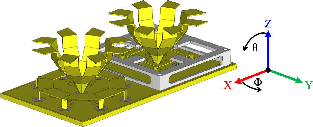
The following multi-antenna module intends to be able to place all antennas in a small area of 114 mm by 56 mm, with a total height of the highest antenna of 26 mm. For the design of such a compressed module, it is necessary that the large wideband antennas for 5G mobile services can be placed above the flat satellite antennas to share the same small area. So, all antennas are performing in a very low volume with each other. In Figure 1, the complete model of the compact automotive multi-antenna system module is pictured. It shows two Palm tree antennas for 5G, which are placed inside the octagonal GNSS Scarabeus ring antenna (front) and the square SDARS Scarabeus antenna (rear), while most of the typical multi-antenna systems have their terrestrial antenna elements next to their satellite antenna elements [Reference Attaran, Larashi, Mäurer and Reddy4, Reference Yacoub and Aloi15]. In the literature, there are only a few contributions that show the function of two or more 5G antennas, which cover the frequency range between 617 MHz and 6 GHz and contain the GNSS bands L1 and L5, to compare with. In Table 1, some of them are shown. As it is not easy to compare different systems with different forms of presentation, the table strives to create a fair comparison. As can be seen, the overall size of our proposed antenna module is one of the examples with the smallest volume requirements. There are some more antenna systems, containing terrestrial and satellite antenna combinations [Reference Nikam and Patil16–Reference Goncharova and Lindenmeier20]. As we can see in Figure 1, the distance between each antenna and the others is very small. This makes it necessary to optimize the physical parameters of every single antenna. In the following sections, we focus on the duality of the Palm tree antennas and a novel dual-band GNSS Scarabeus antenna.

Figure 1.

CST model of the compact multi-antenna module.

Figure 1 Long description

A compact multi-antenna module featuring two Palm tree antennas positioned on a rectangular base. The antennas are depicted with a unique geometric design resembling palm trees, each mounted on separate platforms. The left antenna is placed on a circular platform with multiple cylindrical supports, while the right antenna is situated on a square platform with a grid-like structure. Adjacent to the antennas, a three-dimensional coordinate system is shown with axes labeled X, Y and Z. The X-axis is red, the Y-axis is green and the Z-axis is blue. Two angles, theta and phi, are indicated with curved arrows around the Z and X axes, respectively. The diagram emphasizes the spatial arrangement and orientation of the antennas within the module.

Table 1.

Automotive antenna modules with wideband terrestrial antennas

Table 1 Long description

Rows compare multiple works by PCB size and largest antenna height in millimeters, spacing between terrestrial antennas in millimeters, highest mutual coupling in dB, highest envelope correlation coefficient, whole frequency range in gigahertz without gaps, and applications. Work 7 lists PCB size 122 by 60 with antenna height 22, spacing 60 between middle points and 19.9 between inner edges, mutual coupling less than minus 12 dB, envelope correlation coefficient not given, frequency range 0.617 to 5.5, and applications 5 G, V2X, GNSS L1 and L5, and SDARS. Work 9 lists 120 by 60 with antenna height 52, spacing 19.4, mutual coupling less than minus 9.6 dB, envelope correlation coefficient less than 0.15, frequency range 0.824 to 5.925, and applications LTE, GNSS L1, WLAN, and Wireless Access in Vehicular Environment, WAVE. Work 11 lists 180 by 80 with antenna height 49.5, spacing given as 48.5 by 30 by 49.5, mutual coupling minus 6 dB, envelope correlation coefficient less than 0.4, frequency range 0.617 to 6, and application 2 by 2 5 G MIMO. Work 12 lists shark fin housing size 152 by 58 with antenna height 55, spacing 12, mutual coupling minus 6 dB, envelope correlation coefficient less than 0.3, frequency range 0.698 to 2.69, and applications LTE, FM, and GPS. Work 13 lists 120 by 80 with antenna height 52, spacing not given, mutual coupling values minus 22.1 and minus 23.8 dB, envelope correlation coefficient not given, frequency range 0.698 to 6, and applications LTE, WLAN, V2V, and GNSS L1. Work 14 lists shark fin housing size 160 by 61.5 with antenna height 50 millimeters, spacing not given, mutual coupling less than minus 10 dB, envelope correlation coefficient less than 0.2, frequency range 1.19 to 2.8, and applications LTE, WLAN, and GNSS BeiDou B1. This work lists PCB size 114 by 56 with antenna height 26, spacing 57 between middle points and 12 between inner edges, mutual coupling minus 10.5 dB, envelope correlation coefficient less than 0.05, frequency range 0.617 to 5.925, and applications 5 G, V2X, GNSS L1 and L5, and SDARS.

Palm tree antenna

One basic antenna type of the multi-antenna system is the broadband-capable linearly polarized Palm tree antenna, which acts in a monopole mode. It combines a conical form for wideband coverage of frequencies from 1.4 to 6 GHz with a roof capacitor for coverage of the low-frequency band from 617 to 960 MHz and is easy to realize. Because of the skin effect, the antenna can be designed hollow in the middle, which reduces weight and material. A special property of the antenna is its vertical slots, which make it possible to place circularly polarized ring-like Scarabeus antennas underneath the Palm tree antenna and around their octagonal cones. These slots are sufficient to minimize the influence of the circularly polarized field on the satellite Scarabeus ring antennas.

The current distributions of the two antennas are predominantly orthogonal, as we can see in Figure 2, which reduces electromagnetic coupling between them. This orthogonality minimizes mutual interaction and preserves the individual radiation characteristics of both antennas despite their close spatial integration, thereby enabling the Palm tree antenna to be positioned at the center of the Scarabeus structure. Since the feeding point of the Palm tree antenna is in the center of the ring antenna and since the currents along the ring antenna (yellow) are rotating around it in phase from 0° to 360°, their overall influences on a vertical current at the feed point (red) of the Palm tree antenna compensate each other.

Figure 2.

Schematic visualization of orthogonal current distributions between a Palm tree and a Scarabeus antenna.

The appearance of this specially formed monopole antenna leads to the name “Palm tree.” As in [Reference Panholzer and Lindenmeier7], where a variant of the Palm tree antenna has already been presented, in this contribution, the design develops from a four-level structure to optimize the respective heights in order to minimize mutual coupling effects with other antennas in the proximity of the Palm tree antenna. As it started from a round structure, the cone itself is now designed as an octagonal geometric structure, making it possible to fabricate it from a planar sheet of metal and finally bend it into the final structure and form horizontal elements, which act as a roof capacitor. An evolution of the main Palm tree stages is shown in Figure 3.

Figure 3.

Main evolution steps of the Palm tree antenna.

Figure 3 Long description

Two stages in the evolution of a Palm tree antenna are shown, with dimensions labeled in millimeters. On the left, a smaller antenna structure is shown with several horizontal elements extending outward. The dimensions of these elements are labeled as 8.42 millimeters, 10.71 millimeters and 7.49 millimeters. On the right, a larger antenna structure is depicted, featuring more complex horizontal elements. The dimensions of these elements are labeled as 12.71 millimeters, 10.18 millimeters, 4.30 millimeters and 4.16 millimeters. The central vertical section of the larger antenna is labeled as 45.00 millimeters in height, with a base diameter of 3.56 millimeters. An arrow points from the smaller structure to the larger one, indicating the progression or transformation between the two stages.

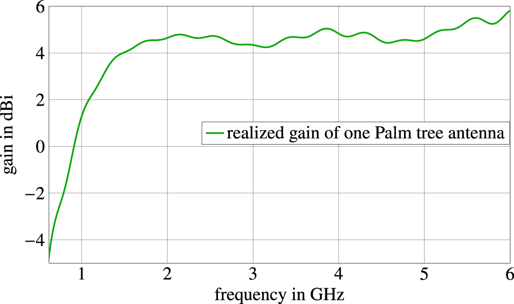
The gain in the horizontal direction for a single simulated omnidirectionally radiating Palm tree antenna is plotted over frequency in Figure 4.

Figure 4.

Simulated realized gain over frequency of one Palm tree antenna at Φ = 270°, Θ = 90°.

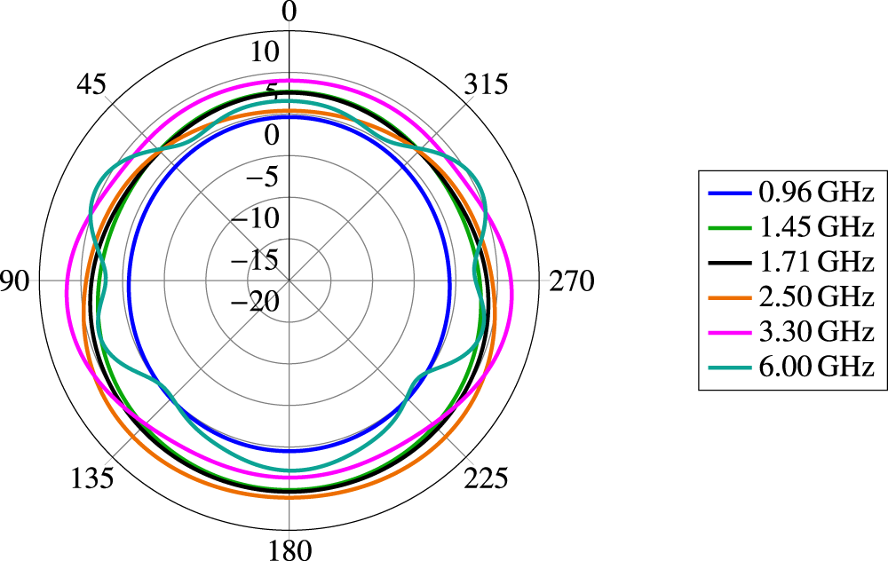
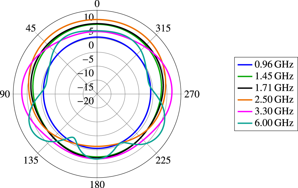
We recognize a low gain in the 5G low-band from 617 to 960 MHz due to the natural mismatch of such a compact monopole-like antenna. To counter this mismatch, the Palm tree antennas are able to use a multi-stage matching network. The realized gain of the Palm tree antennas in the constellation of Figure 1 is plotted in Figure 5 for the Palm tree antenna in the center of the SDARS Scarabeus antenna, and in Figure 6 for the Palm tree antenna in the center of the GNSS Scarabeus antenna.

Figure 5.

Simulated realized gain of the Palm tree antenna inside the SDARS Scarabeus at a cross section of Θ = 90° in dBi.

Figure 5 Long description

Polar plot with angle labels 0, 45, 90, 135, 180, 225, 270 and 315 around the circle. Concentric radial tick labels read 10, 5, 0, minus 5, minus 10, minus 15 and minus 20. A legend at the right lists six line entries: 0.96 gigahertz, 1.45 gigahertz, 1.71 gigahertz, 2.50 gigahertz, 3.30 gigahertz and 6.00 gigahertz. The 0.96 gigahertz curve forms the smallest loop, staying near the 0 ring and dipping inward most strongly around 225 degrees to 315 degrees. The 1.45 gigahertz and 1.71 gigahertz curves form larger, smoother loops between the 0 and 5 rings, with mild outward bulges near 90 degrees and 270 degrees. The 2.50 gigahertz curve tracks close to the 5 ring for much of the circle and is slightly farther out near 135 degrees to 225 degrees. The 3.30 gigahertz curve is the outermost for most angles, running near the 5 to 10 region with a broad, smooth shape. The 6.00 gigahertz curve shows the most variation, with pronounced lobes outward near about 60 degrees and about 300 degrees and deeper inward notches near about 150 degrees and about 210 degrees.

Figure 6.

Simulated realized gain of the Palm tree antenna inside the GNSS Scarabeus at a cross section of Θ = 90° in dBi.

Figure 6 Long description

Simulated realized gain of the Palm tree antenna inside the GNSS Scarabeus at a cross section of Theta equals 90 degrees in dBi. Polar plot with angular axis shown as degrees, labeled 0, 45, 90, 135, 180, 225, 270, 315. Radial axis shows values 10, 5, 0, minus 5, minus 10, minus 15, minus 20. Legend entries list six frequency traces: 0.96 gigahertz, 1.45 gigahertz, 1.71 gigahertz, 2.50 gigahertz, 3.30 gigahertz, 6.00 gigahertz. The 0.96 gigahertz trace forms an almost circular curve close to the 5 ring, with a small outward bulge near 0 degrees and a small inward dip near 180 degrees. The 1.45 gigahertz trace stays between the 5 and 10 rings, closest to the 10 ring near 0 degrees and closer to the 5 ring near 180 degrees. The 1.71 gigahertz trace closely follows the 1.45 gigahertz trace and remains slightly inside it for most angles. The 2.50 gigahertz trace is near the 10 ring around 0 degrees and moves inward toward the 5 ring around 180 degrees. The 3.30 gigahertz trace shows two broad outward bulges near 90 degrees and 270 degrees and a lower section nearer the 5 ring around 180 degrees. The 6.00 gigahertz trace shows multiple lobes and notches, with outward lobes near 135 degrees and 225 degrees approaching the 10 ring and inward notches near 90 degrees and 270 degrees dropping toward the minus 10 ring.

In comparison with some other applications of terrestrial antennas in such close proximity, the radiation patterns show a good omnidirectional behavior with a gain of typically around 4 dB in the horizontal plane and dimples of 0 dB gain at frequencies of more than 5 GHz [Reference Demien and Sarkis21].

Novel GNSS Scarabeus antenna

For GNSS communication purposes, a new Scarabeus-type antenna is deployed. The Scarabeus antenna is a ring antenna with vertical elements in order to shorten the size of the ring. Placed at a distance above the PCB, the Scarabeus antenna performs with low losses as a result of the surrounding air. Through correct design, a Scarabeus antenna is able to cover more L-bands simultaneously [Reference Meredov and Lindenmeier22]. Scarabeus antennas are based on a horizontal ring structure, where, in the resonant radiation mode, one guided wave propagates along the ring structure with one wavelength fitting in. Up to now, four additional vertical elements have been used to shorten the ring while keeping its resonant behavior. The Scarabeus ring structure makes it ideal to be placed underneath a terrestrial antenna of monopole type. As mentioned before, the Palm tree antenna does not disturb the very good performance of Scarabeus ring antennas, even in the case where this wideband antenna totally covers the Scarabeus ring antenna.

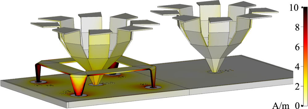
However, the Palm tree antenna itself, which should cover frequencies between 0.6 and 6 GHz, is influenced by resonant modes on the Scarabeus antenna at frequencies close to 3 GHz, where each quarter of the square Scarabeus antenna forms a resonating structure, as can be seen in Figure 9. This behavior can be illustrated very well by the surface current distribution. In Figure 7, we can see the resulting magnitude of the surface current distribution when the left-side Palm tree antenna is excited at 3.1 GHz. The Palm tree antenna induces a surface current at every resonant length of the surrounding four-foot Scarabeus antenna, which also oscillates in monopole mode. Every quarter of the Scarabeus antenna now acts as a parasitic radiator, changing the input impedance of the Palm tree antenna in the center, resulting in a mismatch characteristic.

Figure 7.

Magnitude of surface current distribution in four-foot Scarabeus scenario when the GNSS-side Palm tree antenna is excited at 3.1 GHz.

Figure 7 Long description

The surface current distribution on two antennas mounted on a flat surface. The antennas have a complex geometric structure resembling inverted pyramids with multiple tiers. The left antenna is supported by four legs, each connected to the base, while the right antenna is directly mounted on the surface. A color scale on the right side of the image ranges from 0 to 10 amperes per meter, indicating the magnitude of the surface current distribution. The colors transition from dark red at higher values to yellow at lower values, showing variations in current intensity across the antennas and the supporting structure. The left antenna displays a more intense current distribution at its base and legs, while the right antenna shows a more uniform distribution across its structure.

Figure 8.

CST model of novel octagonal dual-band Scarabeus antenna.

This is why we now introduce a new octagonal concentric Scarabeus antenna with eight vertical elements, as can be seen in Figure 8. For this structure, the same desired resonant behavior is performed for the GNSS frequencies at L1 and L5 bands. But in contrast to the square Scarabeus antenna, higher-order resonances are suppressed, which would harm the performance of the wideband Palm tree antenna.

So, the idea of the new octagonal Scarabeus antenna is to split the resonant length of the resonant quarters of the square Scarabeus antenna by two, as it is illustrated in Figure 9, and to shift the resonance to higher frequencies above 5 GHz.

Figure 9.

CST models of the four-foot dual-band Scarabeus antenna and novel octagon dual-band Scarabeus antenna with comparison of their respective resonant lengths in monopole mode (red) when attached to a Palm tree antenna.

Figure 9 Long description

The image consists of two models of a Scarabeus antenna, each mounted on a square base. The left model shows a central structure with four protruding arms, each connected to a circular pad on the base. Red arrows indicate the flow of current from the central point to the outer pads, illustrating a direct path. The right model is similar but includes additional red arrows forming a loop around the base, indicating a more complex current path. Both models highlight the antenna′s structure and current distribution.

In Figure 9, the two Scarabeus antennas are compared. On the left side, the resonant currents of the square Scarabeus quarters in monopole mode are depicted. Their resonant length is close to λ/4. On the right side of Figure 9, it is visible that the corresponding resonant length of one-eighth of the octagonal Scarabeus is shorter. This way, its resonant frequency is higher. The impact of the resonant length reduction on the surface current distribution can be seen in Figure 10, where we notice an attenuation of the surface current magnitude at the GNSS antenna, while it is high at the Palm tree antenna itself, creating a higher radiation efficiency and total efficiency.

Figure 10.

Magnitude of surface current distribution in the novel octagonal Scarabeus scenario when the GNSS-side Palm tree antenna is excited at 3.1 GHz.

Figure 10 Long description

The surface current distribution on two Scarabeus antennas mounted on a flat base. Each antenna has a complex structure with multiple angular segments extending outward. The left antenna displays a series of angular segments arranged in a circular pattern, while the right antenna mirrors this design. Both antennas are positioned on a rectangular platform with circular mounts beneath them. The surface current distribution is represented by a color gradient scale on the right side, ranging from 0 to 10 amperes per meter, with colors transitioning from lighter to darker shades. The base platform shows circular elements beneath each antenna, possibly indicating mounting points or connectors. The color gradient suggests varying levels of current intensity across the antenna surfaces, with higher values concentrated near the center of each structure.

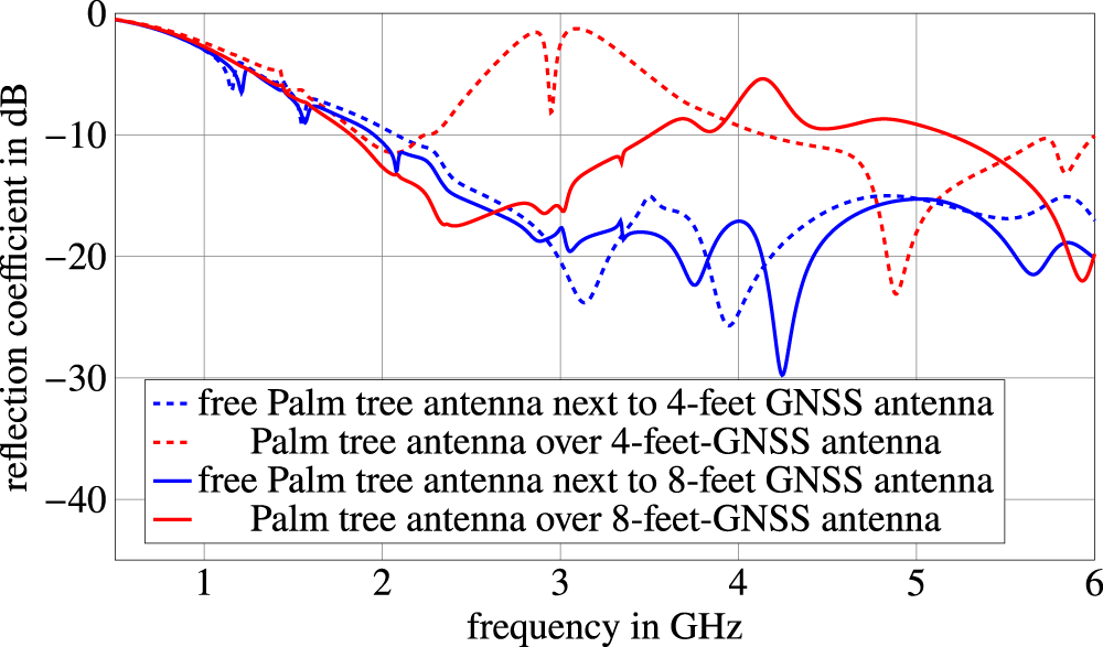
To validate the statement, a direct comparison of the impact of the different Scarabeus types is given in Figure 11. There, the S-parameters of the Palm tree twin antennas are examined when placed in one case inside a four-foot dual-band GNSS antenna, as seen in Figure 7, and in the other case inside the novel eight-foot octagonal dual-band GNSS antenna, as seen in Figure 10. For the comparison, the raw S-parameters of the antenna radiators are shown, without a matching network.

Figure 11.

Comparison of Palm tree twin reflection coefficients in different Scarabeus type scenarios. Reflection coefficient shown for the pure radiators, without a matching network.

As expected, the reduced resonant length leads to an increase in the spurious resonance frequency by 1.3 GHz and an additional suppression of the reflection coefficient by more than 4 dB. An even stronger suppression of the reflection coefficient of the Palm tree antenna inside the GNSS Scarabeus antenna could be achieved by further reducing the coupling-capable resonant length if we use a higher number of vertical elements. The significant improvement qualifies the novel Scarabeus type for deployment under the operating conditions mentioned before.

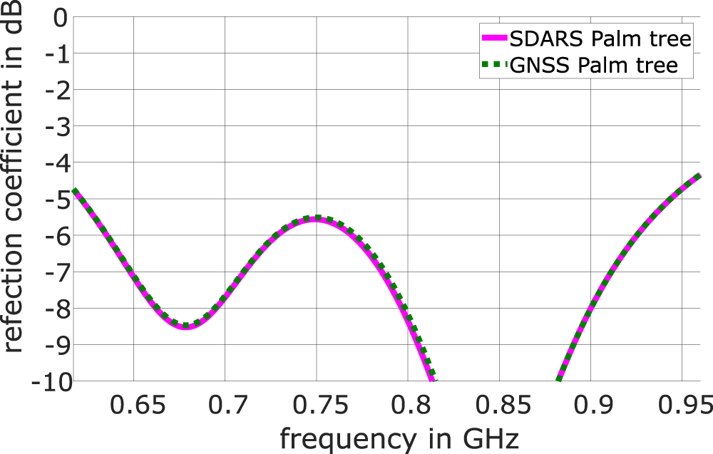
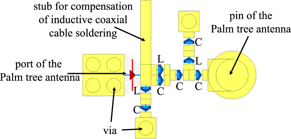
In order to match the Palm tree antennas also at the low-band between 617 and 960 MHz, a further matching network can be included consisting of a series capacitor, a ground connection via, a series resonant circuit and a capacitor, as well as a parallel resonant circuit in series. Figure 12 shows an example of such matching of two Palm tree antennas in the module together with the octagonal GNSS Scarabeus, where the Palm tree antennas have even a 4 mm lower height, still obtaining matching of typically better than −6 dB. The CST layout of this matching network, applied in the overall system from Figure 1, can be seen in Figure 13.

Figure 12.

Example of low-band (617–960 MHz) matching of Palm tree antennas in the module.

Figure 13.

CST layout of low-band (617–960 MHz) multi-stage matching network of the Palm tree antennas in the overall system.

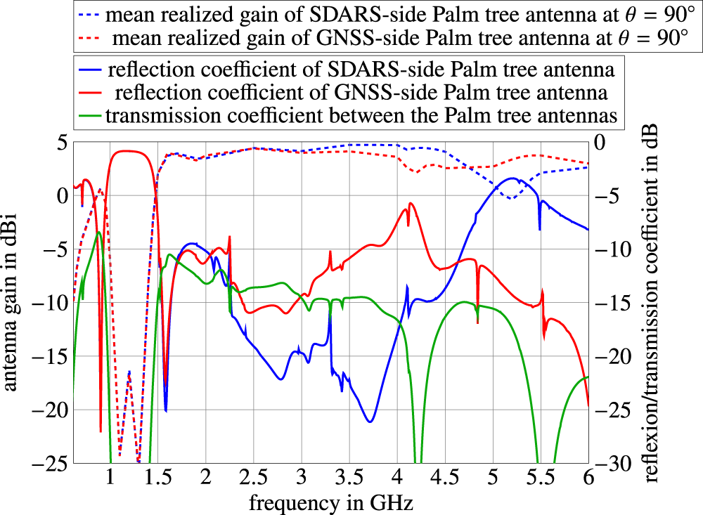
By inserting this matching network into this contribution, we can observe the resulting reflection coefficient and the resulting realized gain of the Palm tree antennas in Figure 14. An optimization of the circuitry is in progress. We also notice good decoupling, mainly lower than −10 dB.

Figure 14.

Reflection coefficient, coupling, and resulting realized gain of the Palm tree antennas with a multi-stage matching network.

Figure 14 Long description

Mean realized gain of SDARS-side Palm tree antenna at theta equals 90 degree Mean realized gain of GNSS-side Palm tree antenna at theta equals 90 degree Reflection coefficient of SDARS-side Palm tree antenna Reflection coefficient of GNSS-side Palm tree antenna Transmission coefficient between the Palm tree antennas. The x-axis is labeled, frequency in gigahertz, with ticks at 1, 1.5, 2, 2.5, 3, 3.5, 4, 4.5, 5, 5.5 and 6. The left y-axis is labeled, antenna gain in decibel isotropic, ranging from minus 25 to 5 with ticks every 5. The right y-axis is labeled, reflexion slash transmission coefficient in decibel, ranging from 0 at the top to minus 30 at the bottom with ticks every 5. Two dashed curves show mean realized gain. The dashed blue curve stays near 3 to 5 decibel isotropic from about 1.6 to about 4.6, then drops to about 0 near 5.2 and rises to about 2 to 3 by 6. The dashed red curve stays near 2 to 4 decibel isotropic from about 1.6 to 6, with a dip to about 2 near about 4.2 to 4.6. Three solid curves use the right y-axis. The solid blue curve is near minus 20 around about 1.6, then varies between about minus 5 and minus 22 from about 2 to 4, then rises toward about minus 2 near about 5.2 and is around minus 6 to minus 8 by 6. The solid red curve is near 0 around about 1.1 to 1.5, then drops sharply near about 1.6, then stays mostly between about minus 8 and minus 15 from about 2 to 5.5 and falls toward about minus 25 by 6. The solid green curve stays mostly between about minus 10 and minus 15 from about 1.7 to 5, with deep notches reaching about minus 30 near about 4.2 and near about 5.5 and is around minus 22 near 6.

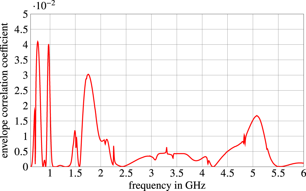
The simulated envelope correlation coefficient (ECC) is shown in Figure 15, which is determined from the S-parameters of the Palm tree antennas with this multi-stage matching network. ECC is a performance criterion for cross-correlation behavior and channel capacity [Reference Kwon, Song and Kim9, Reference Shen, Luo, Miao and Liu14, Reference Vaughan and Andersen23], where values lower than 0.5 at the mobile side are considered to be suitable for MIMO applications. As can be seen in Figure 15, the highest value of ECC is below 0.045 in the considered multi-antenna system, which is caused by its low transmission parameters and a helpful phase difference between reflection and transmission parameters. With that, the multi-antenna system is practicable for MIMO deployment.

Figure 15.

Simulated ECC from the S-parameters of the Palm tree antennas with a multi-stage matching network.

Figure 16.

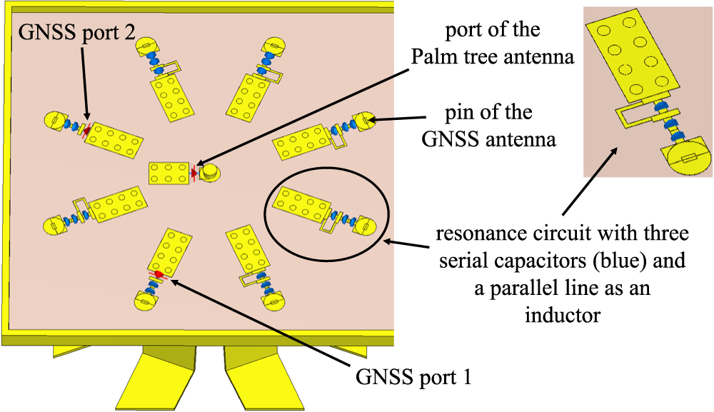
GNSS backside of the PCB with respective circuits and feeds.

Figure 16 Long description

A rectangular board outline contains multiple repeated feed assemblies arranged around a central area. Each assembly shows a rectangular pad with several circular holes, connected by a short trace to a small network made of three serial capacitors and a parallel line and then connected to a circular pad. Text labels identify, GNSS port 2 pointing to one assembly, GNSS port 1 pointing to another assembly, port of the Palm tree antenna pointing to a rectangular pad and pin of the GNSS antenna pointing to a circular pad. One assembly is enclosed by an oval outline and a separate magnified view shows the same enclosed assembly with the rectangular pad, the three serial capacitors, the parallel line and the circular pad. A callout text reads, resonance circuit with three serial capacitors left parenthesis blue right parenthesis and a parallel line as an inductor.

Figure 17.

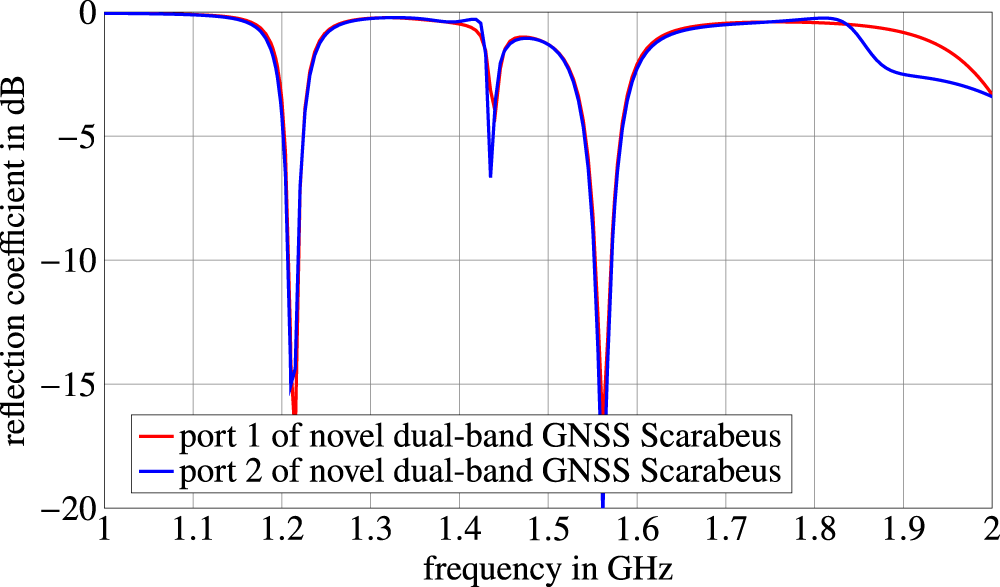
Simulated reflection coefficient of the novel dual-band GNSS Scarabeus at its two ports.

Figure 18.

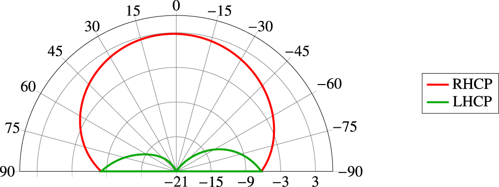
Simulated IEEE gain of the novel octagon GNSS Scarabeus at 1.2 GHz and Phi = 0° in dBi.

Figure 19.

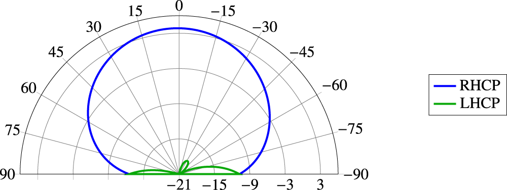
Simulated IEEE gain of the novel octagon GNSS Scarabeus at 1.575 GHz and Phi = 0° in dBi.

Figure 20.

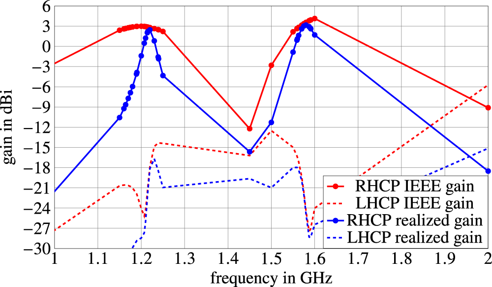
Simulated gain over frequency of the novel dual-band GNSS Scarabeus antenna.

Figure 20 Long description

The x-axis is labeled, frequency in gigahertz, ranging from 1.0 to 2.0 with tick marks at 0.1 intervals. The y-axis is labeled, gain in decibel isotropic, ranging from minus 30 to 6 with tick marks at 3 intervals. A legend lists four series: RHCP IEEE gain, LHCP IEEE gain, RHCP realized gain and LHCP realized gain. RHCP IEEE gain is a solid line with circular markers. It rises from about minus 3 at 1.0 to about 3 near 1.2, then drops to about minus 12 near 1.45, rises to about 4 near 1.6, then decreases to about minus 9 at 2.0. RHCP realized gain is a solid line with circular markers. It rises from about minus 21 at 1.0 to about 3 near 1.22, then drops to about minus 16 near 1.45, rises to about 3 near 1.58, then decreases to about minus 18 at 2.0. LHCP IEEE gain is a dashed line. It is about minus 27 at 1.0, increases to about minus 21 near 1.15, drops to about minus 25 near 1.2, rises to about minus 15 near 1.23, stays around minus 15 to minus 16 through about 1.5, drops to about minus 27 near 1.6, then increases to about minus 6 at 2.0. LHCP realized gain is a dashed line. It is near minus 30 around 1.2, rises to about minus 16 near 1.22, stays around minus 21 to minus 19 from about 1.25 to 1.5, drops to about minus 28 near 1.6, then increases to about minus 15 at 2.0.

Now we consider the performance of the new octagonal GNSS Scarabeus antenna, which is simulated together with the complete antenna module. With just a most unpretentious matching network consisting of series capacitors, recognizable in Figure 16, where the bottom side of the PCB at the GNSS side is pictured, a dual-band matching is realized also for the Scarabeus antenna.

Figure 17 plots the simulated reflection coefficient of the novel dual-band GNSS Scarabeus antenna implemented in the overall system, shown in Figure 1. Figure 18 shows the simulated IEEE gain of the octagonal GNSS Scarabeus antenna when inserted in the overall system at 1.2 GHz. Figure 19 shows the same situation for 1.575 GHz. The performance in the overall system is described with the cross-polarization discrimination (XPD) between right-hand circularly polarized gain and left-hand circularly polarized gain. As we can see, an excellent XPD of more than 20 dB and an axial ratio (AR) close to 1 are achieved even in the presence of the Palm tree antenna. The good XPD is also obtained at the other frequency samples of the proposed frequency bands, as we can see in Figure 20, where the IEEE gain and the realized gain of the novel octagonal dual-band Scarabeus antenna are plotted over frequency.

We notice a broadband XPD behavior at the L1, L2, and L5 GPS bands with a respective high IEEE gain for the right-hand polarization. For this contribution, we decided to use an easy dual-band-capable network because this is sufficient to prove the obtained performance of the novel octagon GNSS Scarabeus antenna while covered by a Palm tree antenna in its center. The radiation efficiency of the dual-band octagon GNSS is in the region of −3 and −4 dB, which is caused by the dual-band resonant network. For single-frequency applications, we get values in the region of −1.5 and −2 dB. In the actual state of the design, there is still potential left to improve the efficiency significantly. More than 20% of the losses are caused by the loss tangent of the cheap FR-4 substrate. Around 10% of the losses are caused by the circuitry, which can be further improved in its design. Also, the metal plating can be changed, which actually leads to 30% of the losses. This way, we can estimate a further increase of 1–2 dB in efficiency for further design iterations.

Measurement of scattering parameters

The scattering parameters of the compact multi-antenna module are measured with a Vector Network Analyzer on an extended ground plane. In Figure 24, we can see the setup for the S-parameter measurement.

Figure 24.

S-parameter measurement setup.

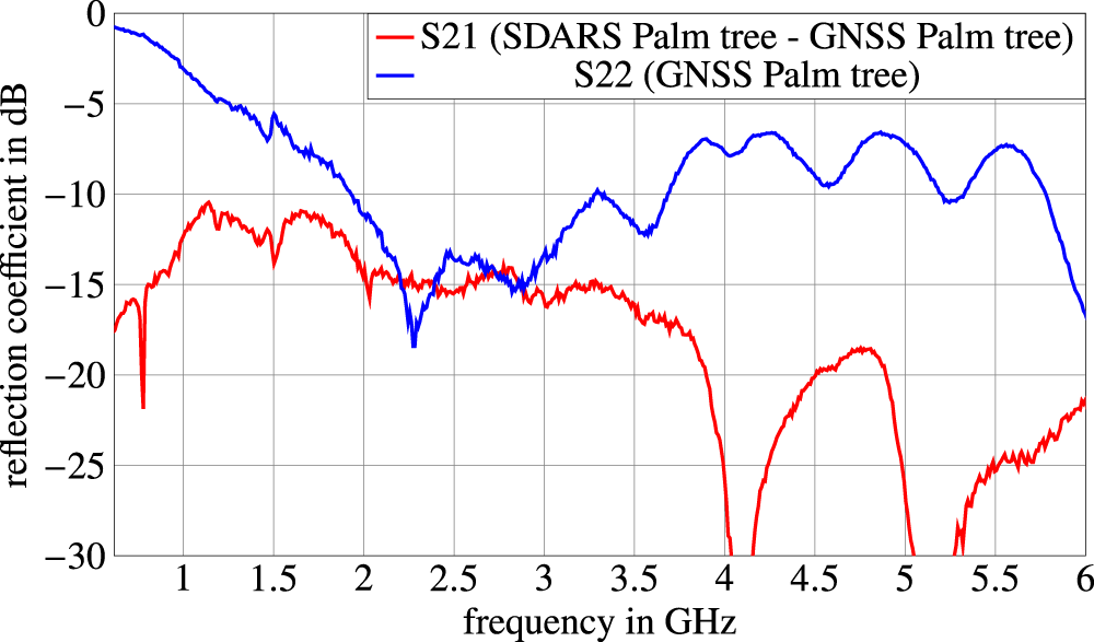
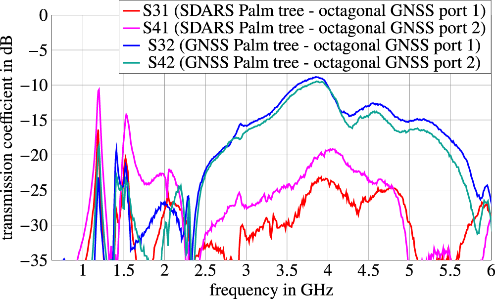
As mentioned before, one of the main challenges of multi-antenna systems in a small accommodation area is the coupling between the respective antennas. Therefore, we have to pay particular attention to the coupling parameters. In Figure 25, we can see the measured transmission coefficient between the linearly polarized terrestrial Palm tree antennas as well as the measured reflection coefficient of the GNSS-side Palm tree antenna.

Figure 25.

Measured S-parameters of Palm tree antennas without a matching network.

Because of the extremely compact module and an antenna distance of only 57 mm, the mutual coupling in this structure is relatively high. But as can be shown by simulation results in Figure 14, the coupling can still be kept mainly lower than −10 dB even with a matching circuit because of its additional losses. For further discussion, we concentrate on frequencies above 1 GHz, due to the usual mismatch of the Palm tree antennas in the 5G low-band, caused by the small height of the antennas. In Figure 25, we can see a coupling of −10 dB at maximum for frequencies up to 2 GHz. For higher frequencies, a coupling of around −15 dB is achieved. For frequencies above 3.9 GHz, transmission coefficients of less than −20 dB are measured. For consideration of the coupling between the new octagonal GNSS Scarabeus antenna and the Palm tree antennas, we look at Figure 26, where we recognize two small band maxima peaks in coupling between the SDARS Palm tree and the octagonal GNSS Scarabeus at 1.196 GHz of −10.7 dB and at 1.53 GHz of −14.2 dB. This is not critical since the 5G antennas are not active at these frequencies.

Figure 26.

Measured transmission coefficients between the Palm tree antennas and the octagonal GNSS Scarabeus.

Figure 26 Long description

Transmission coefficient in decibel. The x-axis is labeled, frequency in gigahertz, with tick labels at 1, 1.5, 2, 2.5, 3, 3.5, 4, 4.5, 5, 5.5 and 6. The y-axis is labeled, transmission coefficient in decibel, with tick labels at 0, minus 5, minus 10, minus 15, minus 20, minus 25, minus 30 and minus 35. A legend lists four curves: S31, S41, S32 and S42. S32 varies from about minus 35 near 1 gigahertz, rises to about minus 10 around 4.0 gigahertz, then decreases to about minus 25 to minus 30 by about 6 gigahertz. S42 follows a similar shape to S32, reaching about minus 10 around 4.0 gigahertz, then decreasing to about minus 30 by about 6 gigahertz. S31 stays mostly between about minus 35 and minus 20, with a broad rise to about minus 23 to minus 24 near 4.0 gigahertz, then drops to about minus 35 near about 5.2 to 5.6 gigahertz and rises again toward about minus 27 near 6 gigahertz. S41 shows a sharp peak near about 1.3 gigahertz at about minus 10, then remains mostly between about minus 30 and minus 20 up to about 4.8 gigahertz, then drops to about minus 35 near about 5.0 to 5.8 gigahertz and rises toward about minus 30 near 6 gigahertz.

For the rest of the frequencies, the antennas are coupled with typically much less than −20 dB. Looking at the coupling between the Palm tree antenna inside the GNSS Scarabeus and the octagonal GNSS Scarabeus, we recognize a peak around 4 GHz with a maximum coupling of slightly more than −10 dB, while at the other frequencies, the antennas are coupled with much lower transmission coefficients. The measurement of the coupling is consistent with the simulated matching of the Palm tree antenna, as shown in Figure 11, where we notice the increase in the reflection coefficient close to 4 GHz.

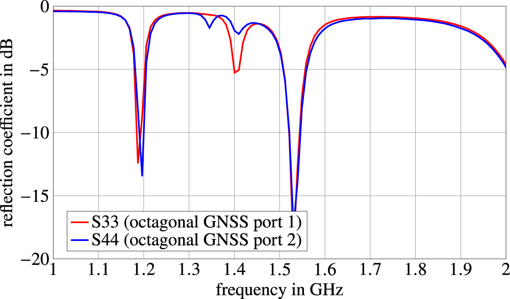
The big advantage of the octagonal GNSS Scarabeus, next to the reduced coupling compared to a four-foot Scarabeus, is its dual-band capability. Therefore, for this antenna, we have to look at the reflection coefficient in Figure 27, where we recognize two peaks with matching character.

Figure 27.

Measured reflection coefficient of the novel octagonal dual-band GNSS Scarabeus.

Compared to the simulated reflection coefficient, illustrated in Figure 17, we see good agreement between the graphs. Some slight frequency deviations of the matched peaks are recognizable, which partly originate from fabrication tolerances of the antennas and elements, as well as parasitic effects of the matching circuits, which consist of resonant circuits, realized in SMD technology. Optimization of the system is in progress.

Measurement of far-field antenna patterns

The far-field measurements are performed in the institute’s anechoic chamber on a finite ground plane with bent edges and a diameter of 1.2 and 4 m of antenna distance. In Figure 28, the measurement setup for the far-field antenna patterns is shown.

Figure 28.

Far-field measurement setup in the anechoic chamber.

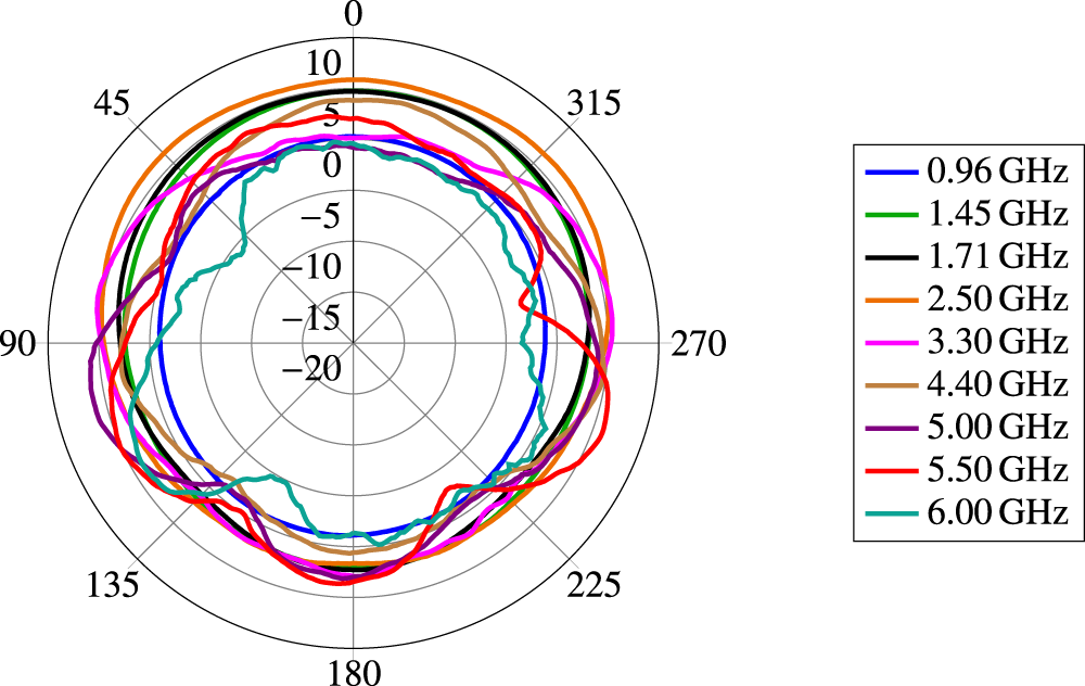
To validate the Palm tree antennas, vertical, horizontal, and half-sphere measurements are performed. Because of the limited ground plane of the measurement setup, the maximum amplitude of the Palm tree antennas is not located at Θ = 90°. Therefore, we look at the vertical plots of the Palm tree antenna inside the octagonal GNSS antenna in Figure 29.

Figure 29.

Measured gain of the Palm tree antenna inside the octagonal dual-band GNSS Scarabeus at different vertical cut sections in dBi.

Figure 29 Long description

Four semicircular polar line plots titled, Phi equals 0 degree, Phi equals 45 degree, Phi equals 90 degree and Phi equals 135 degree. Each plot shows angle in degrees along the arc from 90 degree through 60 degree and 30 degree to 0 degree, then to minus 30 degree, minus 60 degree and minus 90 degree. The radial scale shows values minus 20, minus 15, minus 10, minus 5, 0, 5 and 10. A legend lists six traces labeled 0.960 gigahertz, 1.450 gigahertz, 1.710 gigahertz, 2.500 gigahertz, 3.300 gigahertz and 6.000 gigahertz. Across all four plots, each frequency trace forms two main lobes on either side of 0 degree, with a narrow minimum at 0 degree near the minus 20 ring. For Phi equals 0 degree, the 6.000 gigahertz trace has the most jagged outline and reaches outward to around the 0 to 5 rings near about plus 60 degree and minus 60 degree, then drops toward the minimum at 0 degree near minus 20. The other frequency traces form smoother lobes that stay mostly between the minus 10 ring and the 0 ring, then converge to the same minimum near minus 20 at 0 degree. For Phi equals 45 degree, the two lobes remain centered away from 0 degree and the minimum at 0 degree remains near minus 20. The 6.000 gigahertz trace again extends outward to around the 0 to 5 rings on both sides before returning toward the minimum. The other traces remain mostly between the minus 10 ring and the 0 ring. For Phi equals 90 degree, the lobes are broader in angle, with several traces extending outward to around the 0 ring and slightly above it between about plus 60 degree to plus 90 degree and minus 60 degree to minus 90 degree. The minimum at 0 degree remains near the minus 20 ring. For Phi equals 135 degree, the 6.000 gigahertz trace extends outward to around the 0 to 5 rings near about plus 60 degree, while several other traces extend outward to around the 0 ring over angles from about minus 60 degree to minus 90 degree. The minimum at 0 degree remains near the minus 20 ring.

In Figure 29, we notice a very symmetrical structure of the vertical far-field pattern of the respective frequencies for the four azimuthal cut sections. The roundness is emphasized again in Figure 30, where the horizontal pattern of the Palm tree antenna inside the octagonal GNSS antenna is plotted at an elevation angle of Θ = 70°. As we can notice from the simulated results, the measurement results show an overall good roundness of the radiation pattern with low variance in gain for the respective frequencies. In the direction of the other Palm tree antenna, the gain is slightly decreased by 2 dB, while it is increased by 2 dB in the opposite direction. At higher frequencies, the variances increase, but are still low with respect to the environment of three other antennas.

Figure 30.

Measured gain of the Palm tree antenna inside the octagonal dual-band GNSS Scarabeus at Θ = 70° in dBi.

Figure 30 Long description

Polar plot with angle markings at 0, 45, 90, 135, 180, 225, 270 and 315. The radial scale is labeled 10, 5, 0, minus 5, minus 10, minus 15 and minus 20. A legend lists nine traces: 0.96 gigahertz, 1.45 gigahertz, 1.71 gigahertz, 2.50 gigahertz, 3.30 gigahertz, 4.40 gigahertz, 5.00 gigahertz, 5.50 gigahertz and 6.00 gigahertz. The 2.50 gigahertz trace stays close to the 10 ring for most angles. The 1.71 gigahertz and 1.45 gigahertz traces stay between the 5 and 10 rings for most angles. The 0.96 gigahertz trace stays near the 0 to 5 rings and dips below 0 around the 270 direction. The 3.30 gigahertz, 4.40 gigahertz and 5.00 gigahertz traces mostly lie between the 0 and 10 rings with small undulations. The 5.50 gigahertz trace shows a pronounced outward bulge near 270 and a lower section near 180. The 6.00 gigahertz trace is the most irregular, with multiple inward dips reaching near the minus 10 ring, including around 90 and 270.

Figure 31.

Measured gain of the Palm tree antenna inside the SDARS Scarabeus at Θ = 70° in dBi.

Figure 31 Long description

Polar plot with angular axis shown as degree labels 0, 45, 90, 135, 180, 225, 270, 315. Radial axis tick labels are 10, 5, 0, minus 5, minus 10, minus 15, minus 20, representing gain in decibel isotropic. Legend entries list nine frequency traces: 0.96 gigahertz, 1.45 gigahertz, 1.71 gigahertz, 2.50 gigahertz, 3.30 gigahertz, 4.40 gigahertz, 5.00 gigahertz, 5.50 gigahertz, 6.00 gigahertz. The 2.50 gigahertz trace stays close to the 10 ring over most angles. The 1.45 gigahertz and 1.71 gigahertz traces are generally between 5 and 10 with small undulations. The 0.96 gigahertz trace varies around the 5 ring, dipping toward 0 near 225 and 270. The 3.30 gigahertz trace is near 10 around 90 and 270 and closer to 5 around 0 and 180. The 4.40 gigahertz trace is often between 0 and minus 10, with a broad low region around 180. The 5.00 gigahertz trace is mostly between 0 and 5, with a dip below 0 near 0 and 315. The 5.50 gigahertz trace is mostly between 0 and 5, with a dip toward 0 near 270. The 6.00 gigahertz trace has the deepest notches, reaching about minus 15 near 225 and about minus 10 near 180 and rising toward 5 to 10 near 45 and 90.

Figure 32.

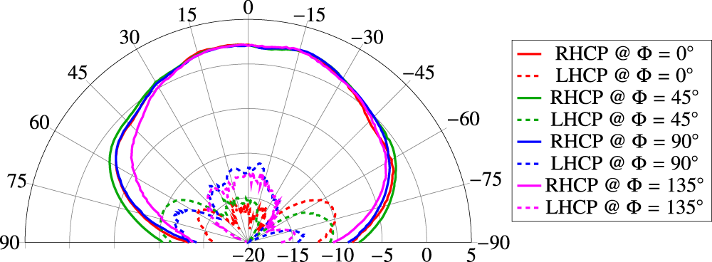
Measured IEEE gain of the octagonal dual-band GNSS Scarabeus antenna at 1.2 GHz in dBi.

Figure 32 Long description

The polar plot illustrates gain patterns for RHCP and LHCP at angles of 0, 45, 90 and 135 degrees. The radial axis represents gain, likely in decibels, ranging approximately from -20 to +5. Solid lines indicate RHCP, while dashed lines indicate LHCP. The red, green, blue and magenta colors correspond to angles of 0, 45, 90 and 135 degrees, respectively. The plot shows dominant lobes with peak gains around 0 degrees and notable sidelobes. RHCP generally exhibits higher gain compared to LHCP, with LHCP being suppressed at certain angles. Key features include peak gain levels and the presence of sidelobes at specific angles, providing insight into the antenna′s directional performance.

Figure 33.

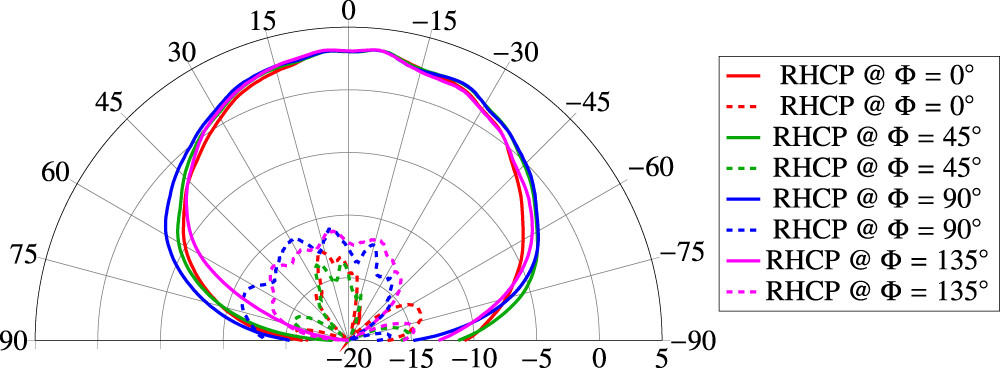
Measured IEEE gain of the octagonal dual-band GNSS Scarabeus antenna at 1.58 GHz in dBi.

Figure 33 Long description

A polar plot with angle markings from 90 through 0 to minus 90. The radial scale is labeled with values minus 20, minus 15, minus 10, minus 5, 0 and 5. No radial axis quantity name or unit is shown. Legend entries list eight traces: RHCP at phi equals 0 degree shown with a solid line and a dashed line, RHCP at phi equals 45 degree shown with a solid line and a dashed line, RHCP at phi equals 90 degree shown with a solid line and a dashed line and RHCP at phi equals 135 degree shown with a solid line and a dashed line. For all four phi values, the solid traces form a broad main lobe centered near 0 degree. The solid traces stay close to the 0 radial ring from about plus 60 degrees to minus 60 degrees, then drop toward the minus 20 radial region as the angle approaches plus 90 degrees and minus 90 degrees. The dashed traces remain in the inner region between about minus 20 and minus 10 on the radial scale. Multiple small lobes are visible between about plus 60 degrees and minus 60 degrees. The dashed traces approach the minus 20 radial region near plus 90 degrees and minus 90 degrees.

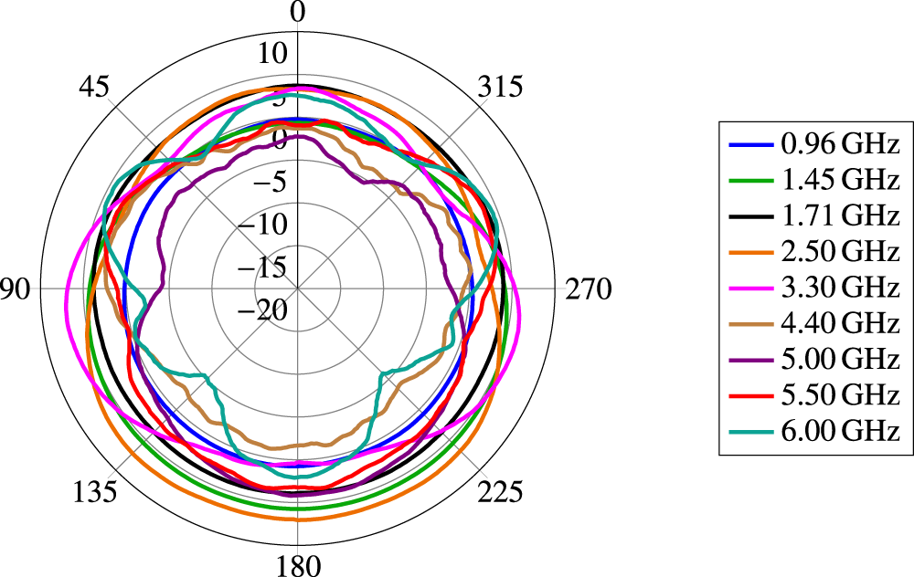
We also get a similarly advantageous radiation pattern with low variance when we look at the Palm tree antenna inside the SDARS Scarabeus. Figure 31 shows the gain of the SDARS side Palm tree antenna, identical in construction, for the same horizontal cut section at Θ = 70°. Here, there is again an increased gain by 2 dB in the opposite direction of the other Palm tree antenna. This way, the slight variances in gain of the two Palm tree antennas complement each other. In summary, the measurements of the Palm tree antennas show good omnidirectional behavior from the point of view of a compact multi-antenna system of this size. It also proves the functionality in combination with the Scarabeus satellite antenna concept. The next measurements concentrate on the novel octagonal dual-band GNSS Scarabeus antenna. The slight frequency shift in good matching of the reflection coefficient, seen in Figure 27, leads to a slight mismatch at the antenna resonance frequencies. Therefore, to show the potential performance of the dual-band Scarabeus antenna, the IEEE gain is plotted. In Figure 32, the IEEE gain of the octagonal dual-band GNSS Scarabeus antenna is plotted for 1.2 GHz, and in Figure 33 for 1.58 GHz.

For both frequencies, we achieve a measured IEEE gain of around 3 dB, while obtaining an XPD of more than 14 dB at 1.2 GHz and 15 dB at 1.58 GHz. The measurements of the novel octagonal dual-band GNSS Scarabeus antenna show very good agreement with the simulated results. Also, the functionality of this antenna concept in combination with a broadband Palm tree antenna is validated.