1. Introduction
Large cooperative robot swarms offer substantial advantages, including decentralization and cost-effectiveness, which generally surpass the challenges brought on by increased system complexity. Decentralization leads to systems that are not only robust against individual failures but also resilient and cost effective to maintain. Moreover, the per-unit cost of individual agents within a swarm is typically lower than that of singular robots designed for comparable tasks, leading to potential savings in both initial investment and long-term operational costs.
Multi-agent systems play a crucial role in mission-critical applications, enabling access to hard-to-reach areas, exploration of hazardous environments, and execution of rescue operations. In search and rescue missions, swarm robots navigate disaster zones, locate survivors, and relay critical information without endangering human responders. In environmental monitoring, they autonomously track pollution levels, map forest fires, and conduct underwater surveillance. The agriculture sector benefits from swarm robotics through precision farming, where coordinated robotic systems optimize planting, irrigation, and harvesting. In industrial automation, swarm robots streamline warehouse logistics, improving inventory management and material transportation. In space exploration, autonomous robotic swarms provide scalable solutions for planetary mapping, extraterrestrial construction, and resource extraction. These diverse applications highlight how swarm robotics enhances efficiency, scalability, and resilience in tackling real-world challenges.
However, the pace of progress in the field of swarm robotics is often hampered by financial and physical constraints. The development of an accessible, small-scale, low-cost, multi-agent robotics platform could significantly enhance research productivity and attract newcomers to the field. Such a platform would serve both as an affordable introduction to swarm robotics and as a versatile testbed for sophisticated algorithms.
Our literature review focuses on a specific niche within distributed robotic systems [Reference Parker1] and swarm robotics [Reference Navarro and Matía2], centering on small-scale (semi-)autonomous mobile multi-robot systems, hereafter referred to as mobile microrobot swarms for brevity. The defining features of these systems include their mobility, albeit potentially limited, and compact size, often just a few cubic inches. These robots, also called agents or units, form a collective, alternatively termed a swarm or group. Each unit is outfitted with a wireless microcontroller to facilitate inter-agent communication and potentially link with external swarm processing nodes, such as a central supervisory computer. The robots possess a degree of autonomy that enables the collective to undertake collaborative tasks or missions. Optionally, agents may be equipped with onboard sensors or actuators, granting them the ability to execute specialized functions, such as detecting chemical plumes or manipulating objects.
The list of systems, platforms, frameworks, and even products we review herein is not exhaustive. We merely aim to offer a historical overview of the technological benchmarks and research trajectories in the field of mobile microrobot swarms over time. The origin of frameworks for swarms of communicating miniature mobile robots dates back to the late 1980s, driven by the ambition to create hardware and software solutions that enable distributed robotic systems. This endeavor aimed to advance research and education in developing algorithms that facilitate cooperative behavior among mobile robots operating at scale. Inherent to microrobots are limitations due to the small size of the swarm units, affecting computational power, energy, mobility range, and the extent of sensing and communication abilities.
One of the pioneering efforts in creating a mobile micro-robot, sized at one cubic inch, was the development of Squirt in the late 1980s by researchers at the Massachusetts Institute of Technology’s (MIT’s) AI Lab [Reference Brooks3–Reference Flynn, Brooks, Wells and Barrett6]. This platform was motivated by educational goals in robotics. Similarly, the Khepera robot, initiated at the Microcomputing Laboratory (LAMI) of the Swiss Federal Institute of Technology in Lausanne (EPFL) in 1991, quickly became a favored tool for collaborative and distributed robotics research over the next three decades. The Khepera IV model [Reference Soares, Navarro and Martinoli7], now discontinued, was priced at $3,200. The initial goal behind the development of both Khepera and Squirt was to advance the miniaturization of mobile robots with respect to sensors, computing, actuation, and power supply rather than focusing on the domain of robot swarms. A noteworthy mention is warranted for the marketable Lego Mindstorms platform [Reference Gindling, Ioannidou, Loh, Lokkebo and Repenning8, Reference Klassner and Anderson9]. Although the Mindstorms “kit” doesn’t strictly belong to the “micro” or swarm robotics category, serving instead as a standardized platform, it represents a significant commercial effort to make robotics educationally accessible and to incorporate robotics into the computing curriculum [Reference Klassner and Anderson9].
Carnegie Mellon University’s Millibot comprised of a heterogeneous team of
 $7^{3}\,{\textrm{cm}}^{3}$
continuous track robots tasked to map and localize within its operational environment [Reference Grabowski, Navarro-Serment, Paredis and Khosla10, Reference Navarro-Serment, Grabowski, Paredis and Khosla11]. Its design philosophy aimed for modularity on a small scale, namely, the ability to conveniently add different capabilities (mostly sensing and less actuating modules) for creating heterogeneous teams. Parallely, the University of Southern California’s Robomote was specifically engineered to enhance power use and efficiency within large-scale, distributed, small-scale robotic systems and sensor networks [Reference Dantu, Rahimi, Shah, Babel, Dhariwal and Sukhatme12, Reference Sibley, Rahimi and Sukhatme13]. Its goal was to facilitate research into expansive mobile sensor networking by employing diminutive units, roughly
 $3.5^{3}\,{\textrm{cm}}^3$
in size, providing functionalities on par with those of larger, more expensive models. The term “mote” refers to low-power sensor nodes integral to distributed sensor networks, attracting substantial research interest in the early 2000s. The concept originates from the aspiring idea of “Smart Dust Motes” – millimeter-sized, low-power nodes designed for sensing and communication – put forward by researchers at the University of California, Berkeley (UCB) [Reference Agogino, Granderson and Qiu14–Reference Wen16]; presumably, as pinpointing its exact origins proves difficult.
The attributes of a mote closely align with those of mobile microrobots, barring the elements of mobility and possibly actuation. The development of TinyOS [Reference Levis, Madden, Polastre, Szewczyk, Whitehouse, Woo, Gay, Hill, Welsh, Brewer and Culler17], an operating system designed for the distinctive requirements of low-power sensing nodes, marks a notable progression derived from mote research at UCB. This example underscores the pivotal importance of specialized software solutions, including unique programming languages, operating systems, or simulation tools, in navigating the intricacies of swarm robotic systems [Reference Pinciroli and Beltrame18, Reference Pinciroli, Trianni, O’Grady, Pini, Brutschy, Brambilla, Mathews, Ferrante, Di Caro, Frederick and Birattari19].
The MICAbot [Reference McMickell, Goodwine and Montestruque20], developed in the early 2000s by the University of Notre Dame, leveraged the MICA platform [Reference Hill and Culler21] from UCB. MICA, a wireless embedded sensor system, served as the wireless microcontroller for these mobile robots. The MICA platform’s appeal lay in its modular suite of sensors, which could be easily attached or detached from the main “mother” interface board.
Concurrently, at UCB’s Sensor & Actuator Center, the CostBots project emerged [Reference Bergbeiter22, Reference Bergbreiter and Pister23]. The developers recognized that the robotic systems available at that time were either prohibitively expensive or excessively specialized, posing challenges for replication. CostBots highlights a miniaturized mobile microrobot platform constructed from off-the-shelf components and open technology, addressing the need for affordable and accessible robotic systems.
Alice [Reference Caprari and Siegwart24], a microrobot platform developed at the Autonomous Systems Lab (ASL) of EPFL, highlighted size as a critical design aspect. With a volume of just
 $2^3\,{\textrm{cm}}^3$
, one of the most miniature systems signified the challenge of integrating locomotion, processing, sensing, and actuation within such compact dimensions. It also introduced the use of Zigbee [Reference Ergen25], a communication radio module operating on TinyOS. Another notable platform is e-puck [Reference lvaro Gutiérrez, Campo, Dorigo, Donate, Monasterio-Huelin and Magdalena26, Reference Mondada, Bonani, Raemy, Pugh, Cianci, Klaptocz, Magnenat, Zufferey, Floreano and Martinoli27], created by GCtronic and three EPFL labs, including the Laboratory of Intelligent Systems and ASL. With currently limited availability in Europe and Asia and a cost of $950, it features a
 $7\,{\textrm{cm}}$
diameter for operating in small desks, a comprehensive sensor array, and an entirely open-source design. E-puck’s “E-Puck Range and Bearing” board facilitates localization of nearby units.
Another example of pursuing miniaturization in communicating mobile robots is Jasmine, which occupies a volume of approximately
 $2.6^{3}\,{\textrm{cm}}^{3}$
. This robot was developed in the early 2010s at the University of Stuttgart [Reference Kernbach28]. Similarly, Bebot, created at the University of Paderborn [Reference Loh and Traechtler29], also maintains a compact design with a volume of roughly
 $9^{3}\,{\textrm{cm}}^{3}$
. A distinctive feature of Bebot is its overhead mechanical platforms, designed to enable collective load transportation through shared effort among swarm members. This capability demonstrates collaboration and swarm actuation, effectively addressing the limitations inherent in individual units.
Rice University’s r-one system [Reference Lynch30, Reference McLurkin, Rykowski, John, Kaseman and Lynch31] was explicitly developed for a problem-based curriculum and educational purposes. The value of this platform extends beyond its design to include resources that facilitate the development of a robotics curriculum. Concurrently, Harvard’s Kilobot [Reference Rubenstein, Ahler, Hoff, Cabrera and Nagpal32, Reference Rubenstein, Ahler and Nagpal33] captured the robotics community’s attention. Kilobot stands out with its distinctive vibrational tripod locomotion mechanism, a single sensor, and a simple yet effective infrared inter-agent communication system. Moreover, its manufacturing cost of $14 positions it as an attractive platform for fostering research in swarm robotics.
In the early 2020s, the Robotarium system from the Georgia Institute of Technology (GaTech) [Reference Pickem, Glotfelter, Wang, Mote, Ames, Feron and Egerstedt34] emerged as a leading example of a remotely accessible multi-robot testbed, allowing users globally to implement and test their algorithms on a physical mobile robot swarm since 2017. The paper by Wilson et al. [Reference Wilson, Glotfelter, Wang, Mayya, Notomista, Mote and Egerstedt35] delivers a comprehensive analysis and assessment of the Robotarium’s user base, detailing demographics, types of experiments conducted, and users’ anticipated outcomes. This study stands out as perhaps the sole contribution that documents and emphasizes the need for and importance of accessibility in mobile multi-robot platforms. Recently, the focus on miniature mobile robotics has pivoted toward transportation systems, with significant research directed toward autonomy and decision-making algorithms that address real-world transportation challenges. Notable ecosystems in this domain include MIT’s Duckietown [Reference Paull, Tani, Ahn, Alonso-Mora, Carlone, Cap, Chen, Choi, Dusek, Yajun and Hoehener36, Reference Tani, Paull, Zuber, Rus, How, Leonard and Censi37], which also offered remote access, and the Scaled Smart City [Reference Beaver, Behdad Chalaki, Zhao, Zayas and Malikopoulos38–Reference Stager, Bhan, Malikopoulos and Zhao40] at Cornell University, epitomizing the research transition towards autonomous transportation systems.
Since the early 2010s, the widespread availability and accessibility of PCB fabrication and 3D printing services, along with desktop printers, have empowered researchers, academic laboratories, and hobbyists to design and develop their own platforms. These platforms, distinguished by unique design, hardware, and software characteristics, often align with the domain of mobile microrobot swarms, either fully or partially. Notable examples include Carnegie Mellon’s Finch [Reference Lauwers and Nourbakhsh41], Arizona State University’s Pheeno [Reference Wilson, Gameros, Sheely, Lin, Dover, Gevorkyan, Haberland, Bertozzi and Berman42], Parallax’s Scribbler [Reference Tran43], Pololu’s 3pi [Reference Thursky and Gaspar44], and iRobot’s Create [Reference Correll, Bachrach, Vickery and Rus45].
This comprehensive, albeit not exhaustive, overview of platforms encapsulates the defining notions and design traits of mobile microrobot swarms, enabling us to confidently derive certain observations, insights, and conclusions. These conclusions are drawn from online resources and research literature corresponding to nearly three decades of development efforts by numerous institutions and small companies, primarily in North America and Europe.
In essence, the quintessential and indispensable attributes of a mobile microrobot swarm include compactness, affordability, mobility, and capabilities in communication and autonomy. At the system level, it is crucial for the agents (robots) to possess real-time localization within their operational environment (arena), and for the system to exhibit scalability, meaning it should seamlessly support a large number of units. Additionally, the platform must be accessible and thoroughly documented.
A significant body of research literature, which utilizes mobile multi-robot experimental testbeds to validate theoretical findings on topics pertinent to distributed control or estimation in multi-robot systems and swarm behavior, underscores the need for such platforms. Furthermore, from an educational standpoint, there is a global drive toward introducing robotics and programming to increasingly younger audiences.
Presently, only a single system (e-puck) is commercially available on a limited number of continents, while several platforms – such as Khepera and Kilobot – have been phased out from the market. This scenario suggests that these systems do not present a viable commercial opportunity, given that the demand, although present, is insufficient to sustain their production and distribution. Therefore, there is a palpable discrepancy between the availability and the demand for mobile microrobot swarm systems.
Moreover, literature suggests a preference among end-users either to purchase or to construct their own systems. The challenge of replication, particularly in the context of manufacturing, acts as a deterrent. Users generally favor purchasing affordable components over undertaking their own fabrication efforts. Despite the availability of numerous platforms offering detailed instructions and blueprints, actual replication is rare. This can be attributed to several factors, including limited access to fabrication tools (e.g., 3D printers) or the requisite expertise to operate them. Consequently, purchasing low-cost components, such as a robot chassis, emerges as a more viable and practical option. Additional barriers that render experimental testbeds for such systems inaccessible include limited laboratory space, a lack of expertise (e.g., in electronics, programming, CAD design), and issues related to affordability.
In light of the discussed need, significance, availability, barriers to accessibility, and end-user preferences, we introduce the ArachneFootnote 1 System: our proprietary open-access mobile microrobot swarm experimental testbed platform. This initiative, presented in this paper, represents the culmination of approximately ten years of research into developing computer-controlled, small-scale, affordable robotic platforms, targeting the educational engagement of high school and undergraduate students with mobile and swarm robotics. Notably, the platform was inclusively developed by first-year engineering and computer science undergraduate students, aiming to acquaint students with the then-emerging fields of networked control and cyber-physical systems. Through the development process, the platform serves as an introductory tool for students, merging concepts from communications, embedded programming, control systems, and robotics into a cohesive learning experience.
At the heart of the Arachne System are the Arachne Bots, centimeter-scale mobile robots characterized by their engaging design, minimal assembly time, low cost, and availability of parts. The system utilizes globally accessible off-the-shelf components, which can be sourced from both toy and electronics stores. In this paper, we pinpoint the essential building blocks required to construct a mobile microrobot swarm, ensuring that developers can substitute unavailable parts with equivalent alternatives. This approach allows for the replication of our design into customized systems that align with individual budgets and specifications.
Moreover, we demonstrate how straightforward electronic modifications can enhance the sensory capabilities of the Arachne Bots. Our contribution includes a suite of algorithms facilitating a range of behaviors, from basic tasks like set-point convergence and individual robot object manipulation to more complex collective actions such as collision avoidance and group object manipulation. We have articulated the control logic in an accessible manner, eliminating the need for an in-depth understanding of control theory or robotics.
This endeavor seeks to make research in mobile robotic swarms more inclusive, offering a platform that can be developed with little to no specialized knowledge. Our goal is to inspire the broader community in the creation of custom testbeds, original peripherals, and control algorithms for mobile microrobot swarms, thus democratizing the field for researchers, students, and enthusiasts alike.
The physical architecture and design of the Arachne Bots are explored in Section 2, where we detail its subsystems and components. The development of a miniaturized proximity sensor for the Arachne Bots is outlined in Section 3. Mathematical modeling principles governing the Arachne Bots are elucidated in Section 4, providing insight into their movement and control mechanisms. The same section is dedicated to the exposition and analysis of several control algorithms for various system tasks. An empirical assessment of the Arachne Bots’ performance, demonstrating their practical capabilities, is presented in Section 5. Finally, Section 6 offers concluding observations on the platform.
2. Design and architecture
Arachne Bots, an overhead camera, and a laptop computer comprise the Arachne System. The overhead camera serves as the main motion sensor, while the supervisory controller is executed on the laptop computer. The Arachne Bots themselves consist of four basic subsystems: a chassis and transport mechanism, motion sensors, a microprocessor, and a radio component. The four subsystems constitute the essential, bare minimum, structural components required to assemble a mobile and cooperative multi-robot system. Each Arachne Bot takes roughly
 $90$
min to assemble, costs approximately
 $\$80$
, and has a volumetric footprint of about
 $12\,{\textrm{cm}}^{3}$
.
2.1. Body and motors
Mechanical components of the Arachne Bots were obtained from the commercially available Spider toy robot by HEXBUG [46]. The HEXBUG’s Spiders are six-legged arthropods that are powered using two DC motors. The Arachne Bots’ controlled DC motors control forward motion and heading. Figure 1 shows the front view of an Arachne Bot. HEXBUG is a consumer robotics line developed by Innovation First International to complement the VEX Robotics Design System [47]. In January 2023, Spin Master Corp. acquired the HEXBUG brand, expanding its portfolio of creative robotic technology.
Front view of the arachne bot. The main body is obtained from HEXBUG’s toy robot, spider. A protoboard with a small footprint is placed on top of the robot’s chassis. The protoboard mounts the wireless microcontroller. The latter generates the control signals that operate the robot’s motion.

The frame of the HEXBUG Spider was selected due to its engaging bio-inspired appearance with the objective of stimulating the interest of younger audiences. The robot’s hexapedal locomotion can accommodate mildly uneven terrains, exceeding many other centimeter-scaled, hard-wheeled, mobile robots. However, the system is versatile enough to support different types of drive systems, such as differential wheels or steering configurations. An alternative commercially available differential drive robotic chassis, that was used for the system, can be seen in Fig 2.
The wireless microcontroller of the arachne bot is attached to a differential drive chassis.

2.2. Wireless microcontroller
Each Arachne Bot is remotely controlled by the panStamp low-power wireless microcontroller [48]. The panStamp was selected due to its low cost, small footprint, and radio capabilities. It is programmed from the Arduino open-source Integrated Development Environment (IDE), which incorporates numerous libraries that can accommodate low-level operations. A significant volume of documentation and code is accessible online for the Arduino, which has been produced by the large community that supports this platform.
Adruino’s easy-to-use tools and programming language significantly reduce the development time of the Arachne System, making it accessible to users with limited experience in computer engineering. The second significant advantage of the panStamp is its ability to function as a transceiver rather than only a transmitter or receiver. To this end, the control algorithms can be executed from a central supervisory controller or distributively between the wireless mobile nodes. The ability of the Panstamps to function as either simple transmitter-receiver pairs, or as a more complex network, is an essential strength of the Arachne System. These varied capabilities make the platform accessible for researchers or students with limited communication experience, while still allowing for complex communication networks.
Central to the panStamp is an
 $8\,{\textrm{MHz}}$
Atmel Atmega 28P MCU. RF communication (frequency:
 $868/915\,{\textrm{MHz}}$
, baud rate:
 $38400$
) is integrated using a Texas Instruments CC1101 RF interface with a line-of-sight range of up to
 $200\,{\textrm m}$
.
2.3. Webcam-based agent tracking
Each Arachne Bot is tracked using Roborealm [49], a commercially available visual software application. The overhead camera captures the top view of the planar workspace containing the Arachne Bots. The software is able to track predetermined markers known as fiducials. The fiducial marker is placed on top of the rigid bodies (Arachne Bots or objects), parallel to the plane, in order to be fully visible by the overhead camera. The visual tracking system serves as a virtual Global Positioning System (GPS), localizing each Arachne Bot in the workspace (arena). The rate at which the pose (position and heading) measurements are captured ranges between
 $20$
to
 $30\,{\textrm{fps}}$
. These data are then further broadcasted to each Arachne Bot at a rate of
 $100\:\,{\textrm{Hz}}$
. The area Roborealm scans is approximately
 $3{\textrm m}\times 1{\textrm m}$
. However, the size of the viewed area can be controlled by changing the camera’s vertical position. The testing setup, including the camera and the robots, is shown in Fig. 3.
Camera apparatus and testing area. In the existing system, the overhead camera is placed approximately
 $1.6\;{\textrm m}$
from the floor resulting in a
 $3\,{\textrm m}\times 1\,{\textrm m}$
visible arena.

In the Arachne System, Roborealm transmits the pose measurements to each agent individually through a Python script that is executed to a central panStamp transmitter. The overhead video sensor used in the experiments was an inexpensive Logitech Photo ID webcam. A personal license for Roborealm costs
 $\$49.95$
, and an academic license is even less costly with a price of
 $\$39.95$
. The Roborealm software, overhead camera, and central panStamp transmitter were connected to a laptop computer. The central computer collects the pose data of each robot and transmits this information to each robot. In a centralized configuration (mission, scenario, or experiment), the central computer executes the supervisory controller controlling the individual agents.
2.3.1. Electronics
A Texas Instruments DRV8833 motor driver commands the motion of the Arachne Bots. This PWM-based motor driver is ideal due to the integrated over-current and over-temperature protection circuit, and its wide range of operational voltages. The motor driver controls both DC motors with a voltage range between
 $2.7\,{\textrm V}$
and
 $10.8\,{\textrm V}$
. The PWM inputs to the DRV8833 motor driver control the motor speed and direction. The Arachne Bots are powered by lithium-ion polymer (LiPo) batteries that incorporate an onboard charging station. The charging station also includes an LED power indicator light and a power switch.
The LiPo batteries used with the Arachne Bots output
 $3.7\,{\textrm V}$
from a supply of
 $850\,{\textrm{mAh}}$
, which offers approximately three to four hours of battery life. The battery chargers can accept power via a micro-USB port at either
 $3.3\,{\textrm V}$
or
 $5\,{\textrm V}$
. The batteries themselves can plug into the chargers using a JST and receive a maximum current of
 $100\,{\textrm{mA}}$
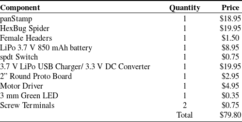
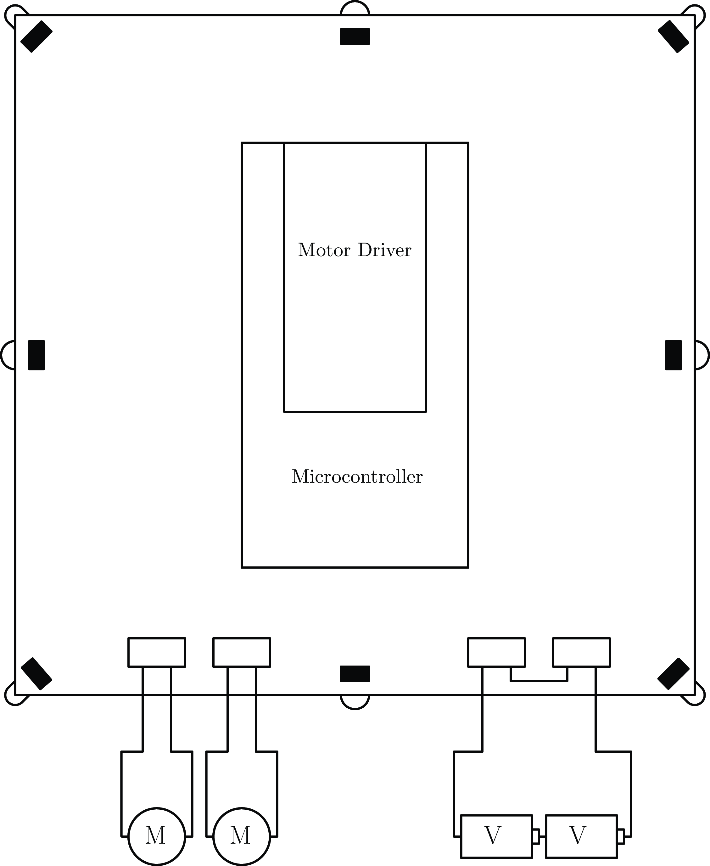
. If on-board charging is unnecessary for a particular project, this circuit could be removed to reduce cost. Table I outlines the individual parts and their cost for a single Arachne Bot. The schematic for the standard Arachne Bot board is illustrated in Fig. 4.
Electronic components and their cost for a single Arachne Bot.

Schematic of the standard Arachne Bot board. The main components are the panStamp wireless microcontroller, the DRV8833 motor driver, and the voltage regulator.

Unlike the vast majority of existing small-scale multi-robot systems, the entire manufacturing process of the Arachne Bots is performed on a simple through-hole protoboard. Therefore, there is no need for machine assembly or extensive soldering experience. Any home user with access to a basic soldering kit could easily assemble an Arachne Bot without any additional training. This not only helps reduce the cost of construction but it also allows complete beginners to assemble Arachne Bots with ease.
3. Sensor Extension: the infrared beacon
The Arachne Bot can be configured to operate using different sensory or maneuverability attachments. One such extension is the InfraRed (IR) sensing beacon board. The beacon functions as an on-board perception module placed on each individual locomotive agent. It can be used to measure both the range and bearing of neighboring Arachne Bots or its surroundings locally. Its functionality resembles the operation of a primitive LiDAR system (Light Detection and Ranging). Compared to other available multi-agent robotic systems, the Arachne Bot’s IR Beacon (IRB) provides a very low-cost method of implementing cooperative control algorithms on mobile robotic collectives. This section describes how the standard board can be modified to incorporate an on-board IR perception module.
3.1. Hardware overview
The IRB board consists of eight emitter-receiver pairs operating at a wavelength of
 $940\,nm$
arranged on top of, and below the board, at
 $45^{\circ }$
intervals as shown in Fig. 5. The SEN-00241 receivers are straight-facing and have an operational field-of-view of approximately
 $45^{\circ }$
. This allows for the beacons to detect
 $360^{\circ }$
of infrared light (separated to eight sectors). When an infrared source is in range, exactly one receiver will detect the signal with little to no dead zones or overlap.
Representation of the IR Beacon Board. In our design, the board acts as an interface shield, connecting the microcontroller to the power source and the two motors.

The 7OED-EL-1L2 emitters are high-powered infrared LEDs chosen due to their high intensity and low power consumption. With the microcontroller output of
 $3.3\,{\textrm V}$
, the receivers can detect the emitters at distances of up to
 $15\,{\textrm{cm}}$
, which is an ample range for a
 $3\,{\textrm{cm}}$
by
 $3\,{\textrm{cm}}$
robot. The emitters are installed under the beacon facing outwards. Since the receivers and emitters are placed on top of, and under the board, respectively, each pair can be mounted at the same orientation on the beacon without the risk of an agent detecting itself. This setup also allows the boards to detect collisions with reflective walls and surfaces, as well as the imminent occurrence of other agents.
The emitters are connected in parallel to one digital output pin of the microcontroller. Using the built-in analog voltage sensing capabilities of the unit, the sensor readings can range from
 $0$
to
 $1023$
with a sampling rate of
 $10\,{\textrm{kHz}}$
. These measured values correspond to a voltage interval from
 $0\,{\textrm V}$
to
 $5\,{\textrm V}$
, meaning that each point is equivalent to approximately
 $4.9\,{\textrm{mV}}$
. Low and high readings correspond to high and low-intensity signals, respectively.
The board is powered by two lithium-polymer batteries with terminal voltages of
 $3.7\,{\textrm V}$
. The full
 $7.4\,{\textrm V}$
supply is used to power the infrared receivers and motor driver which both require at least
 $5\,{\textrm V}$
to operate accurately. The board also contains a voltage regulator which reduces the voltage to
 $3.3\,{\textrm V}$
in order to power the microcontroller. The full wiring schematic for the IRB can be found in Fig. 6.
Wiring schematic for the Arachne Bot IRB board. This extension module is equipped with emitter-receiver pairs that provide each Arachne Bot on-board perception capabilities. Each bot can detect adjacent obstacles and agents.

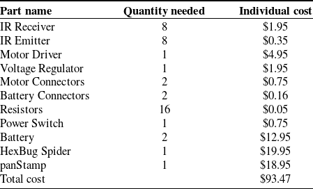
Even though printed electronics were used for the IRB board, the same circuit can be easily assembled with a simple through-hole protoboard (much like the standard Arachne Bot board) without sacrificing size or usability. Table II shows a price breakdown of each individual component of the Arachne Bots IRB.
Electronic components and their cost of an arachne bot with the IRB board.

3.2. Measurements
Three tests were performed to ensure the accuracy and usability of the IRB hardware. The first two tests investigate the localization capabilities of the IRB boards. The use of a local coordinate system requires two types of measurements: range and bearing. Range determines how far away a neighboring agent is located, and bearing determines its relative heading. A third test was also performed to determine the amount of noise or interference detected by the infrared receivers.
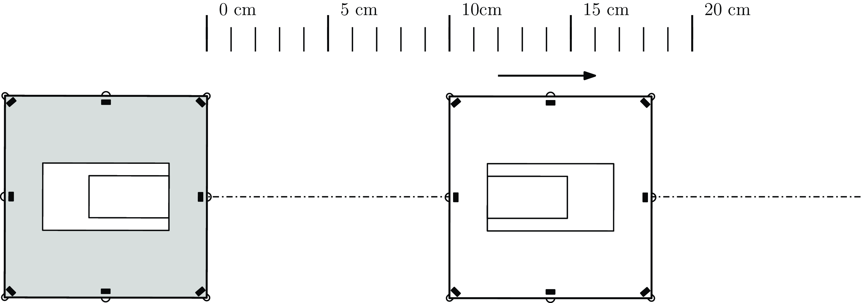
Each test was performed using two IRB boards on a flat surface. In order to measure range, an emitter beacon was kept stationary while a receiver beacon was moved apart from the emitter incrementally. The range measurements were performed at a constant bearing with the two North emitters of the two beacons facing each other. The receiving beacon was then moved back from
 $0\,{\textrm{cm}}$
to
 $18\,{\textrm{cm}}$
at increments of
 $1\,{\textrm{cm}}$
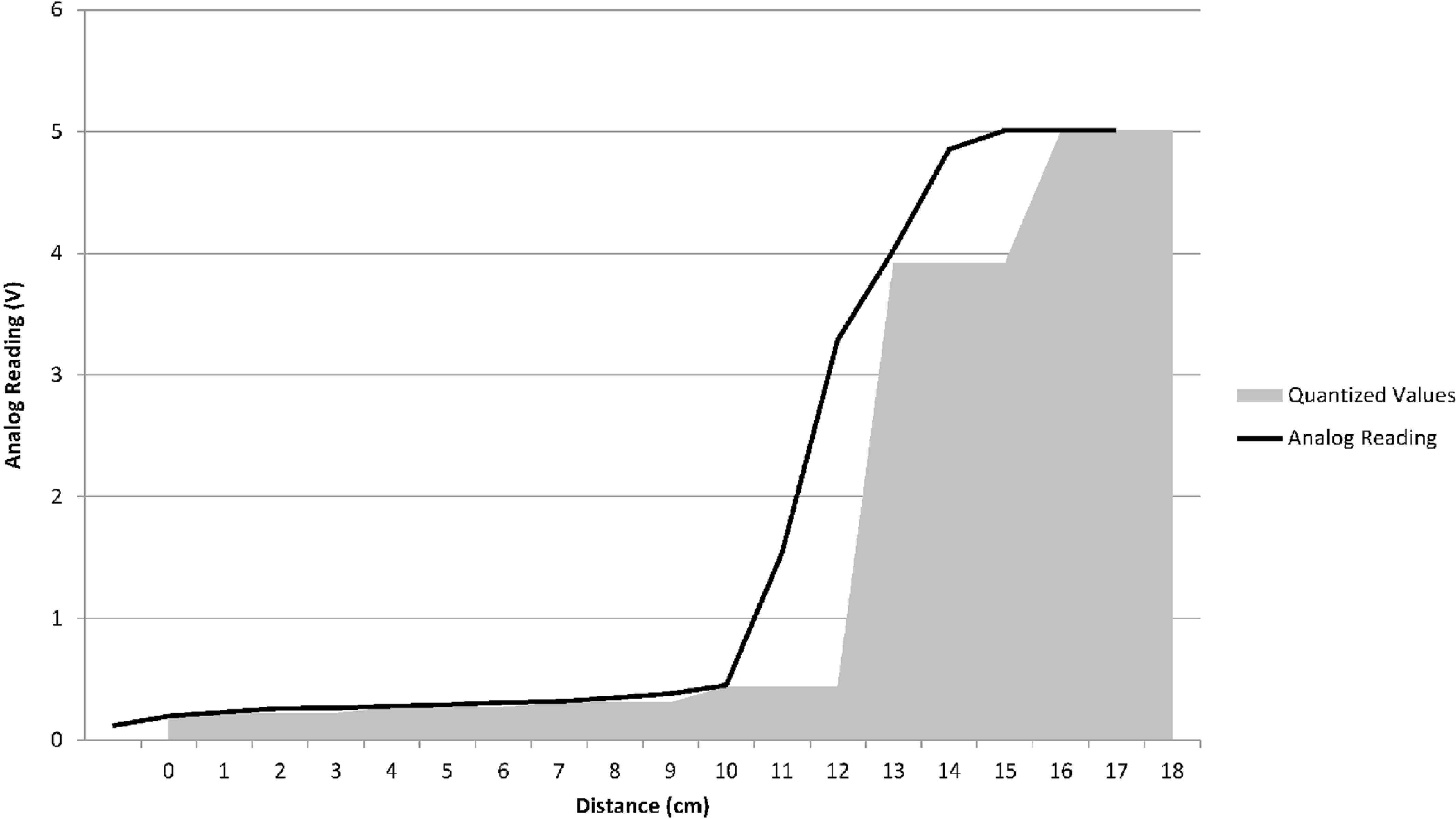
. Figure 7 illustrates the experiment with corresponding results presented in Fig. 8. All graphical data are inverted for ease of viewing, meaning that a low reading corresponds to a low-intensity signal. The microprocessor uses a nonlinear quantized scale to determine the range in centimeters. Figure 9 shows the quantized values that the microprocessor uses along with the raw analog voltage reading attained.
Diagram of range test. The receiver beacon (white) is moving apart from the emitter beacon (grey), in increments of
 $1\,{\textrm{cm}}$
while retaining constant heading.

Range measurements from the receivers of the IRB board.

Range map of the IRB board. The distance readings are not linear. In the chart, the dark line represents the analog voltage readings on the north pin, while the shaded areas mark the quantized distances which the microprocessor translates these readings from.

The verification of the direction bearing was performed at a distance of
 $6\,{\textrm{cm}}$
with the emitting board kept stationary, while the receiving board was rotated in
 $10^{\circ }$
increments through a full rotation. The experiment procedure is illustrated in Fig. 10, and the receiver readings can be found in Fig. 11.
Diagram of bearing test. The receiver board (white) is rotated in increments of
 $10^{\circ }$
relative to the emitter board (gray). The relative range between the two boards is kept constant to
 $6\,{\textrm{cm}}$
.

Bearing measurements from the receivers of the IRB board.

The final experiment was performed using a method that was very similar to the range test. The boards were placed on a level surface facing one another and starting at a distance of
 $1\,{\textrm{cm}}$
. From there, they were gradually separated in intervals of
 $3\,{\textrm{cm}}$
. At each of these distances, the analog voltage reading was recorded about
 $1500$
times over a period of around
 $3$
min. The results of this experiment prove that there is very little noise or interference. In fact, not even one point of deviation was measured over distances up to
 $13\,{\textrm{cm}}$
. These results indicate that the beacons detect very little noise, removing the need to filter the infrared sensor signals.
4. Analytical foundations of the system: kinematic analysis, control principles, and task execution algorithms
This section describes some fundamental analytical background related to the motion of the Arachne Bots. In addition, it provides a series of engaging algorithms that involve both individual and collaborative behavior of the Arachne System. The objective is to provide an analytical description of the Arachne Bots motion and also set some benchmark routines that can be used for object manipulation and group-collaborative tasks.
We emphasize that the algorithms described herein are relevant to small-scale planar mobile robots across different locomotion configurations, extending beyond the Arachne System. Their design is intuitive, aiming to be accessible without necessitating an extensive knowledge of control systems theory.
4.1. Arachne Bot kinematics
The legs of the Arachne Bot are equivalent to a nonslipping driving wheel. Its steerability is controlled by the rotation of its torso. The Arachne Bot maneuverability is similar to a differential-drive or unicycle-like robots. The robot’s kinematics constitute a nonholonomic system that has a first-order, non-integrable constraint [Reference Kanayama, Kimura, Miyazaki and Noguchi50]. As a result, the Arachne Bots’ motion cannot be described as omnidirectional.
Two reference frames are introduced to illustrate the Arachne Bots’ planar kinematic equations. The reference frames are defined using the center and two orthogonal unit vectors. First, the fixed inertial (global) reference frame is
 $\mathcal{F}_{I}=\left \{ O_{I},\vec {i}_{I},\vec {j}_{I}\right \}$
. The second reference frame is a moving body-fixed reference frame, defined as
 $\mathcal{F}_{B}=\left \{ O_{B},\vec {i}_{B},\vec {j}_{B}\right \}$
. This reference frame origin,
 $O_{B}$
, is the center of gravity body (CG) of the Arachne Bot. A traditional right-handed Cartesian coordinate system
 $\left \{ \vec {i}_{B},\vec {j}_{B}\right \}$
is constructed using a vector,
 $\vec {i}_{B}$
, which points forward and a vector
 $\vec {j}_{B}$
which points to the left aft side as shown in Fig. 12.
The polar coordinate system, inertial and body-fixed reference frames, and the heading angles defined from cartesian to polar coordinate transformation. The angle
 $\sigma$
represents the LOS of the robot.

The posture vector,
 $p=\left [x;y;\psi \right ]$
, fully defines the robot’s planar 2-D motion. Here,
 $x$
,
 $y$
represent the inertial frame Cartesian coordinates, and the robot’s heading is
 $\psi$
. By definition, the two frames
 $\mathcal{F}_{I}$
and
 $\mathcal{F}_{B}$
are aligned when
 $\psi =0$
. The combination of angular velocity,
 $\omega$
, and linear velocity,
 $v$
, controls the robot’s locomotion. The standard unicycle-like robot kinematics are
 \begin{align} \dot {x} & =v\cos \psi ,\nonumber \\ \dot {y} & =v\sin \psi ,\nonumber\\ \dot {\psi } & =\omega . \end{align}
The linear and angular velocities are controlled by regulating the voltage of the two DC motors on board the Arachne Bot. For simplicity, we assume a static map between the velocities of the robots and its motors, that is,
 \begin{align}&\, v =K_{v}V_{{{legs}}}, \end{align}
 \begin{align}& \omega =K_{\omega }V_{{{torso}}}, \end{align}
where
 $K_{v}$
and
 $K_{\omega }$
are positive gains, and
 $V_{{{legs}}}$
and
 $V_{{{torso}}}$
are the voltages that regulate the motion of the legs and the torso of the Arachne Bot, respectively.
4.2. Set-point control (move to a target location)
The stabilization challenge of non-omindirectional robots has been thoroughly investigated [Reference Kanayama, Kimura, Miyazaki and Noguchi50–Reference Samson and Ait-Abderrahim53]. The goal is to move the robot to the null posture
 $[0;0;2n\pi ]$
with
 $n\in \mathbb{Z}$
. Robot stabilization with non-holonomic constraints is presented in Kolmanovsky’s survey paper [Reference Kolmanovsky and McClamroch54].
In the context of the Arachne System, set-point control is considered a less analytically complex modulation of the stabilization law. Hereafter, we only need the inertial reference frame,
 $\mathcal{F}_{I}$
, to define coordinates. The goal is to have the robot navigate to a reference target location
 $\left (x_{t},y_{t}\right )\in \mathbb{R}^{2}$
in the 2-D plane, referred to as the set-point or waypoint. The robot is not required to have a certain heading when it reaches the target set-point.
Our subsequent algorithms for collision avoidance and object manipulation use a high-level paradigm that calculates reference waypoints for robotsFootnote 2 in a discrete-time or -event manner. This method is standard for the “task” or “mission” control layer, generating commands that define a velocity profile or waypoint. The subordinate set-point control algorithm ensures the robot converges on these waypoints within a practical timeframe by adjusting its linear and angular velocities. The lower-level motor and steering control layer, as delineated in (2) and (3) for the Arachne System, maps linear and angular velocity profiles into voltage signals for the robot’s motor(s) and steering mechanism. This foundational layer aligns with the robot’s electromechanical configuration that defines its maneuverability [Reference Siegwart and Nourbakhsh55]. This hierarchical control architecture enables the high-level algorithms, specifically those for collision avoidance and object manipulation, to be not only applicable to the Arachne System but also adaptable and hardware-agnostic with respect to the mobile robot platforms on which they are implemented.
We adopt a modified version of the set-point control law presented in ref. [Reference Lee, Cho, Hwang-Bo, You and Oh56]. Essentially, the algorithm is a formal version of the intuitive principle of “turn and move-towards-the-target” approach. The controller is expressed with respect to the polar coordinates, instead of the standard Cartesian form:
 \begin{alignat} {2} \rho & =\sqrt {\left (x-x_{t}\right )^{2}+\left (y-y_{t}\right )^{2}} & \;\;\; & \psi _{t}=\textrm {atan2}\left (y_{t}-y,x_{t}-x\right ). \end{alignat}
Here, the coordinates
 $\rho$
and
 $\psi _{t}$
represent the relative distance and heading, respectively, between the Arachne Bot and the target. The error between the robot’s current heading and the target is
 $\alpha =\psi _{t}-\psi$
. The three coordinate systems are illustrated in Fig. 12.
The set-point control problem requires that the coordinates
 $\left (\alpha ,\rho \right )$
will asymptotically converge to one of the equilibrium points
 $\left (0,2n\pi \right )$
with
 $n\in {{\mathbb{Z}}}$
as
 $t\rightarrow \infty$
. This requires that the target is aligned with the heading of the robot (
 $\alpha \rightarrow 2n\pi$
), and that the robot converges to the target (
 $\rho \rightarrow 0$
). After the coordinates change (from
 $x$
,
 $y$
to
 $\rho$
,
 $\alpha$
), the robot’s kinematics become
 \begin{align}&\,\,\, \dot {\rho } =-\cos \alpha \cdot v, \end{align}
 \begin{align}& \dot {\alpha } =\sin \alpha \cdot \frac {v}{\rho }-\omega . \end{align}
A quick inspection of the kinematics illustrates that a singularity occurs when
 $\rho =0$
. This incidence takes place due to the ambiguity introduced by the definition of
 $\texttt {atan2}({\cdot },{\cdot })$
when
 $\left (x,y\right )=\left (x_{t},y_{t}\right )$
. When the control law is implemented, this singularity is eliminated. Furthermore, in practical, real-world implementations, algorithm execution is terminated once the robot enters a circular disk of the set-point of radius
 $R_{t}$
. The feedback control law is similar to that presented in ref. [Reference Wilson, Glotfelter, Wang, Mayya, Notomista, Mote and Egerstedt35]:
 \begin{align} v & =K_{\rho }\cos \alpha \cdot \rho ,\nonumber \\ \omega & =K_{\rho }\cos \alpha \cdot \sin \alpha +K_{\alpha }\sin \alpha , \end{align}
where
 $K_{\rho }$
and
 $K_{\alpha }$
the positive valued gains. This differs from [Reference Wilson, Glotfelter, Wang, Mayya, Notomista, Mote and Egerstedt35] because
 $K_{\alpha }\sin \alpha$
is used rather than the simpler proportional term
 $K_{\alpha }\alpha$
. In our approach, all angles are channeled through trigonometric functions to eliminate the discontinuous jumps that take place by the definition of
 $\psi _{t}$
and the measurement range of
 $\psi$
.
The stability of the control law is established using the following Lyapunov function:
 \begin{equation*} V(\rho ,\alpha )=\frac {1}{2}\rho ^{2}+\left (1-\cos \alpha \right ) \end{equation*}
which is positive definite for
 $\rho \neq 0$
and
 $\alpha \neq 2n\pi$
where
 $n\in \mathbb{Z}$
. Taking the derivative of
 $V(\rho ,\alpha )$
with respect to time along the system trajectories yields:
 \begin{align*} \dot {V} & =-\cos \alpha \cdot \rho \cdot v+\sin \alpha \cdot \left (\sin \alpha \cdot \frac {v}{\rho }-\omega \right )\\ & \stackrel {\text{(7)}}{=}-K_{\rho }\cos ^{2}\alpha \cdot \rho ^{2}-K_{\alpha }\sin ^{2}\alpha \lt 0\\ &\text{ for }\rho \neq 0\text{ and }\alpha \neq 2n\pi \text{, }n\in \mathbb{Z}. \end{align*}
The derivative of
 $V(\rho ,\alpha )$
is negative definite. The resulting equilibrium points
 $\left (0,2n\pi \right )$
, with
 $n\in \mathbb{Z}$
, are asymptotically stable.
When the heading error equals
 $2n\pi$
, the robot aligns with the target. According to the control law in (7), the advancement
 $v$
turns negative if
 $\cos \alpha \lt 0$
. When that happens, the Arachne Bot reverses until its heading aligns with the target. To ensure forward movement only, conditional logic is applied, enabling positive advancement when the target falls within the robot’s line-of-sight (LOS), represented by the angle
 $\sigma \in \left (0,\;\frac {\pi }{2}\right ]$
. In this case, pure rotation without advancement occurs if
 $\left |\alpha \right |\gt \sigma$
or
 $\cos (\alpha )\gt \cos (\sigma )$
, with control velocities as follows:
 \begin{equation*} v=0; \quad \omega =\begin{cases} -\omega _{0}, & \sin \alpha \geq 0,\\ \omega _{0}, & \text{otherwise}, \end{cases} \end{equation*}
where
 $\omega _{0}\gt 0$
denotes a constant angular velocity. When
 $|\alpha |\lt \sigma$
, the feedback control law reverts to (7), ensuring a positive (forward) advancement
 $v$
as
 $\cos \alpha \gt 0$
in this heading error,
 $\alpha$
range. The pseudocode for this set-point control law is detailed in Algorithm 1.

4.3. Collision avoidance
Collision avoidance is frequently encountered in real-world multi-robot applications. Deconfliction algorithms should be used by each robot on the team to guarantee collision-free missions. These collision avoidance algorithms can take many forms including optimization and force fields [Reference Kuchar and Yang57]. We present an intuitive, distributed deconfliction algorithm to validate the collaborative behavior and group constraints of Arachne Bots.
Consider a workspace containing
 $n$
mobile robots (Arachne Bots), mathematically represented as the index set
 $\mathcal{N}=\left \{ i=1,\ldots ,n\right \}$
. A target location
 $\left (x_{t}^{i},y_{t}^{i}\right )\in \mathbb{R}^{2}$
,
 $i\in \mathcal{N}$
, is prescribed to each robot. When two robots,
 $i$
and
 $j$
, are separated by a distance that is less than some critical value,
 $R_{c}$
, a conflict has occurred:
 \begin{equation*} \rho _{i,j}\leq R_{c}\textrm{, where}\quad \rho _{i,j}=\sqrt {\left (x^{i}-x^{j}\right )^{2}+\left (y^{i}-y^{j}\right )^{2}}. \end{equation*}
An intermediate, reference location for each robot,
 $\left (x_{r}^{i},y_{r}^{i}\right )\in \mathbb{R}^{2}$
,
 $i\in \mathcal{N}$
, is defined within the collision avoidance algorithm. The following equality
 $\left (x_{r}^{i},y_{r}^{i}\right )=\left (x_{t}^{i},y_{t}^{i}\right )$
, holds true when no conflict occurs. At each execution instant, robot
 $i$
determines the set of conflicting robots, which is defined as
 $\mathcal{D}_{i}=\left \{ j\in \mathcal{N}-\left \{ i\right \} :\rho _{i,j}\leq R_{c}\right \}$
. In a real-world application, the set
 $\mathcal{D}_{i}$
can be identified by an onboard proximity sensor on robot
 $i$
, such as the infrared beacon described in Section 3. If a single sensor measures the absolute position of each robot, the set
 $\mathcal{D}_{i}$
is determined by calculating the relative distance between each robot
 $i$
and the remaining
 $n - 1$
robots in the swarm.
Robot
 $i$
’s relative heading angles with respect to (conflicting) robots belonging to
 $\mathcal{D}_{i}$
are
 \begin{equation} \psi _{i,j}=\textrm{atan}2\left (y^{j}-y^{i},x^{j}-x^{i}\right ). \end{equation}
The above definition yields
 $\psi _{j,i}=\psi _{i,j}-\pi$
. Note that robot
 $i$
’s reference heading to the target (4) is by definition
 \begin{equation} \psi _{t}^{i}=\textrm{atan}2\left (y_{t}^{i}-y^{i},x_{t}^{i}-x^{i}\right ). \end{equation}
The algorithm partitions the radius
 $R_{c}$
circular disk with origin at robot
 $i$
, denoted by
 $A_{i}$
, into
 $S$
equal circular sectors,
 $S_{i}^{k}$
,
 $k=1,\ldots ,S$
, with central angles
 $s=2\pi /S$
. When a conflict arises, indicated by a nonempty set
 $\mathcal{D}_{i}$
, the
 $S$
circular sectors are sequentially scanned to locate the first one that is empty, meaning it does not contain any conflicting robots. The first sector,
 $S_{1}$
, is defined such that its bisection is aligned with the line that connects robot
 $i$
with its target location, and the reference location is set equal to the target location, i.e.,
 $\left (x_{r}^{i},y_{r}^{i}\right )=\left (x_{t}^{i},y_{t}^{i}\right )$
. Assuming that the first sector is empty of conflicting robots, robot
 $i$
moves toward the target location. Otherwise, the second sector is scanned, and if, in turn, this sector is empty, the reference location becomes the point where the bisection of
 $S_{2}$
intersects the margin of
 $A_{i}$
.
Overall, the scanning sequence continues until a sector
 $S_{i}^{k}$
is found free of conflicting robots in
 $\mathcal{D}_{i}$
. When this is the case, the reference point of robot
 $i$
,
 $\left (x_{r}^{i},y_{r}^{i}\right )$
, is set equal to the intersection point of the bisection of the sector
 $S_{i}^{k}$
with the circular margin of
 $A_{i}$
, such that we have
 \begin{align} x_{r}^{i} & =x^{i}+R_{c}\cos \left [\psi _{k}^{i}\right ]\: & y_{r}^{i}=y^{i}+R_{c}\sin \left [\psi _{k}^{i}\right ], \end{align}
where
 \begin{equation} \psi _{k}^{i}=\psi _{t}^{i}+\left (k-1\right )\frac {2\pi }{S}\text{ for }k\in \mathcal{N} . \end{equation}
Figure 13 shows schematically the sector partitions of
 $A_{i}$
. Segment
 $S_{k}^{i}$
is deemed collision free when for
 $j\in \mathcal{D}_{i}$
we have
 \begin{equation} \cos \left (\psi _{i,j}-\psi ^{i}\right )\lt \cos \left (\pi /S\right ). \end{equation}
The conflict disk,
 $A_{i}$
, characterized by a radius
 $R_{c}$
, is segmented into
 $S$
circular sectors. During each iteration of the algorithm, these sectors are examined in sequence to locate a sector devoid of collisions. The sector identified as collision-free, denoted as
 $S_{i}^{k}$
, where
 $k\in \{1,\ldots ,S\}$
, is designated to include the reference location
 $(x_{r}^{i},y_{r}^{i})$
.

When a robot finds itself encircled by conflicting agents, meaning all circular sectors are occupied, it opts to remain stationary by setting its coordinates
 $(x_{r}^{i},y_{r}^{i})$
to its current location
 $(x^{i},y^{i})$
. The choice of how many partitions
 $S$
to divide the disk
 $A_{i}$
into is a critical design parameter that influences the algorithm’s behavior and performance. A higher number of partitions enhances the probability of identifying an unoccupied sector for the robot to move toward, yet it concurrently escalates the algorithm’s computational load and run time.
Our approach delineates a specific movement strategy for the robots: each seeks the earliest unoccupied “corridor” to its right for navigation. This prescribed movement pattern induces a collective, macroscopic behavior akin to the counterclockwise flow observed in a cyclone, leading the swarm, when observed as a whole, to exhibit rotational motion. Robots situated on the perimeter of this cyclonic formation are thus able to locate a clear path toward their designated targets. The pseudocode detailing this collision avoidance mechanism is presented in Algorithm 2.

The algorithm can be executed either centrally, in a supervisory controller, or distributively, on each robot. In the central execution, the supervisory controller receives the coordinates of all robots and determines the reference coordinates for each robot to ensure collision-free motion. In the distributed execution, each robot independently uses its global coordinates and sensory data, such as from a proximity sensor (e.g., the IRB board), to compute its desired reference coordinates.
In terms of complexity, the central execution has a time and space complexity of
 $O(nS)$
, where
 $n$
is the number of robots and
 $S$
is the number of sectors. Conversely, the distributed execution reduces the complexity to
 $O(S)$
.
4.4. Object manipulation
Incorporating object interaction capabilities into mobile robots significantly enhances their functionality and adaptability in diverse environments. We describe an algorithmic procedure that enables Arachne Bot to perform a form of object manipulation. Specifically, the algorithm allows a planar mobile robot to push a round object from any initial position to a designated target position,
 $\mathcal{T}:\left (x_{t},y_{t}\right )\in \mathbb{R}^{2}$
.
During object manipulation, the robot persistently re-positions itself so that the object lies between the robot and the target. It then walks toward the target, pushing the object as it goes. Let
 $\mathcal{O}:\left (x_{o},y_{o}\right )\in \mathbb{R}^{2}$
denote the geometric center of the object and its coordinates. The contact point is determined by a position vector from the object to the target. This position vector, along with its unit vector, is given by
 \begin{equation*} N_{o}=\left [\begin{array}{cc} x_{o}-x_{t}; & y_{o}-y_{t}\end{array}\right ]\quad \textrm {and}\quad \hat {n}=\left [\begin{array}{cc} n_{x}; & n_{y}\end{array}\right ], \end{equation*}
where
 $\hat {n}=N_{o}/\left \Vert N_{o}\right \Vert$
. The point of contact,
 $\mathcal{C}$
, between the object and the robot is determined by the unity vector
 $\hat {n}$
as well as a positive coefficient
 $\mu _{o}$
, representative of the radius (or size) of the object. The position of
 $\mathcal{C}$
, in the inertial reference frame is given by
 \begin{equation*} \mathcal{C}:\left (C_{x},C_{y}\right )=\left (x_{o}+\mu _{o}\cdot n_{x},y_{o}+\mu _{o}\cdot n_{y}\right ). \end{equation*}
To circumvent an untimely collision with the object before reaching point
 $\mathcal{C}$
, the robot’s reference point is adjusted to first direct it toward an inline point,
 $\mathcal{I}$
, prior to proceeding to
 $\mathcal{C}$
. Similar to
 $\mathcal{C}$
,
 $\mathcal{I}$
is located along the line that connects the target with the object. However,
 $\mathcal{I}$
is positioned further from the target compared to
 $\mathcal{C}$
. The position of
 $\mathcal{I}$
is determined analogous to
 $\mathcal{C}$
. The location of
 $\mathcal{I}$
is defined as
 \begin{equation*} \mathcal{I}:\left (I_{x},I_{y}\right )=\left (x_{o}+\mu _{I}\cdot n_{x},y_{o}+\mu _{I}\cdot n_{y}\right ), \end{equation*}
where the coefficient
 $\mu _{I}$
, which is largest than
 $\mu _{o}$
, specifies its distance from the object.
When the robot commences the manipulation procedure from a position between the target and the object, it is instructed to execute a sidestep maneuver to one of two auxiliary reference points,
 $\mathcal{A}$
or
 $\mathcal{B}$
, situated in the aft vicinity of the object. This maneuver is a precursor to the previously outlined procedure. Points
 $\mathcal{A}$
and
 $\mathcal{B}$
are defined with the same safe distance
 $\mu _{I}$
of
 $\mathcal{I}$
such that no premature collisions occur when the robot approaches the object. The waypoints
 $\mathcal{A}$
and
 $\mathcal{B}$
are given by
 \begin{align*} \mathcal{A}:\left (A_{x},A_{y}\right ) & =\left (x_{o}-\mu _{I}\cdot n_{x},y_{o}+\mu _{I}\cdot n_{y}\right )\\ \mathcal{B}:(B_{x},B_{y}) & =\left (x_{o}+\mu _{I}\cdot n_{x},y_{o}-\mu _{I}\cdot n_{y}\right ) \end{align*}
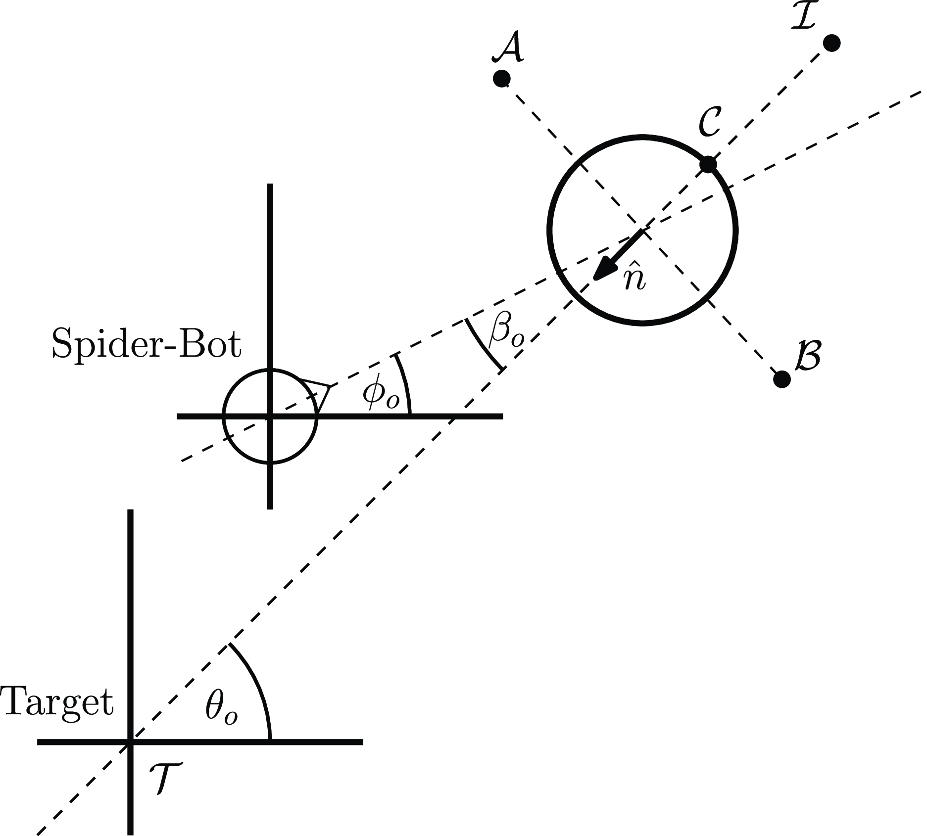
Figure 14 illustrates all the waypoints described so far. The sequence of waypoints that the Arachne Bot moves through is governed by the angle,
 $\beta _o$
, which is determined by the difference between the line segment connecting the robot to the object and the one connecting the target to the object. This angle
 $\beta _o$
is calculated as the difference between the relative angle of the object with respect to the robot,
 $\phi _o$
, and the relative angle of the object with respect to the target,
 $\theta _o$
. These angles are computed as follows:
 \begin{align*} \theta _{o}&=\textrm {atan2}\left (y_{o}-y_{t},x_{o}-x_{t}\right ),\\ \phi _{o}&=\textrm {atan2}\left (y_{o}-y,x_{o}-x\right ), \end{align*}
and
 \begin{equation*} \beta _{o}=\phi _{o}-\theta _{o}. \end{equation*}
Representation of waypoints and relative angles involved in the object manipulation algorithm.

The choice of the waypoint sequence – either (
 $\mathcal{I}$
,
 $\mathcal{C}$
) or (
 $\mathcal{A}$
or
 $\mathcal{B}$
,
 $\mathcal{I}$
,
 $\mathcal{C}$
) – depends on the robot’s initial position relative to the quadrants defined by the line through points
 $\mathcal{A}$
and
 $\mathcal{B}$
and the line connecting the target with the robot, as depicted in Fig. 15.
Halfplanes and their corresponding conditions determining the sequence of waypoints for the object manipulation algorithm. The selection between waypoints
 $\mathcal{A}$
or
 $\mathcal{B}$
is dictated by the sign of
 $\sin \beta _o$
.

If the robot starts in the half-plane opposite the target, demarcated by
 $\mathcal{A}$
and
 $\mathcal{B}$
, the condition
 $\cos \beta _{o}\lt 0$
applies, and the robot adheres to the sequence (
 $\mathcal{I}$
,
 $\mathcal{C}$
). Otherwise, it follows the sequence (
 $\mathcal{A}$
or
 $\mathcal{B}$
,
 $\mathcal{I}$
,
 $\mathcal{C}$
). The choice between
 $\mathcal{A}$
and
 $\mathcal{B}$
as the initial waypoint hinges on the sign of
 $\sin \beta _o$
;
 $\mathcal{A}$
is chosen if
 $\sin \beta _o\gt 0$
; otherwise, the sequence starts with
 $\mathcal{B}$
. The task is deemed completed when the relative distance between the object,
 $\mathcal{O}$
, and the target,
 $\mathcal{T}$
, falls below a tolerance threshold,
 $\epsilon _{t}$
.
The pseudo-code for this procedure is shown in Algorithm 3. At each step of the pseudo-code, a waypoint is generated. The set-point control algorithm, detailed in Section 4.2, is then utilized to guide the robot toward these waypoints.

4.5. Group object manipulation
Advancing from single-robot to multi-robot manipulation, this section presents an algorithm for a team of four Arachne Bots to transport a rectangular box with known dimensions. This algorithm enables the coordinated effort required for the robots to push the box to a specified target location and orientation, represented as
 $\mathfrak{T}:\left [\mathcal{T},\theta _{t}\right ] \in \mathbb{R}^{2} \times \left [0,2\pi \right )$
where
 $\mathcal{T}:\left (x_{t},y_{t}\right )\in \mathbb{R}^{2}$
, from any initial configuration of the robots and the box.
The specified challenge merges swarm robotics [Reference Wang and Schwager58] with the classical computational challenge known as the “piano movers” problem [Reference Canny59, Reference Schwartz and Sharir60], which involves moving an object from one point to another within a plane containing geometric constraints, such as walls.
The core strategy involves the robots encircling the box in a calculated, equiangular arrangement to ensure effective caging and transportation. Caging, a method where robots form a perimeter around an object to control its movement, is fundamental for achieving the desired position and orientation [Reference Brown and Jennings61–Reference Yamada and Saito65]. In our approach, the movement toward the target is facilitated through waypoints, which guide the robots through three main phases: pathing (initial positioning), translation (moving towards the target location), and rotation (adjusting to the target orientation). In the subsequent analysis, it is necessary to define an object-fixed frame, denoted as
 $\mathcal{F}_{B}=\{\mathcal{O},\vec {i}_{B},\vec {j}_{B}\}$
.
The origin of the frame,
 $\mathcal{O}$
, is positioned at the geometric center of a rectangular box. The basis vectors
 $ \{\vec {i}_{B}, \vec {j}_{B}\}$
are aligned with the symmetry axes of the box, with
 $ \vec {j}_{B}$
preferably oriented along the symmetry axis corresponding to the length or longer side of the rectangular object.
Pathing
The pathing phase entails the determination of the robots’ initial approach waypoints in relation to the object, contingent upon the object’s orientation. Initially, we define the orientation angle of the object,
 $\theta _{b}$
, within the inertial reference frame, leading to the segmentation of the plane into quadrants based on this angle. Subsequently, approach points are delineated at a fixed distance,
 $\rho _{a}$
, from the object. These points are evenly distributed, with angular increments of
 $\frac {\pi }{2}$
radians commencing from
 $\theta _b$
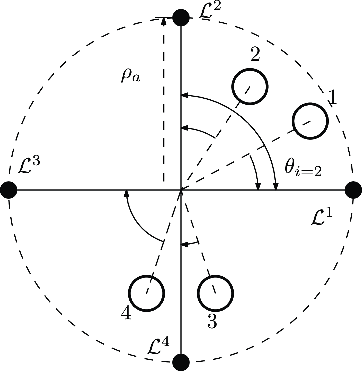
. Figure 16 depicts the four waypoints used to position the robots around the box (object). The approach distance,
 $\rho _{a}$
, is required to exceed half of the box’s larger dimension – whether width or length – by a factor of at least two.
Approaching robot waypoints,
 $\mathcal{L}^{i}$
with
 $i\in \{1,2,3,4\}$
, around the object during the pathing phase of the algorithm. The robots are distributed around the object in
 $\pi /2$
increments starting from the object’s orientation
 $\theta _b$
in the reference frame.

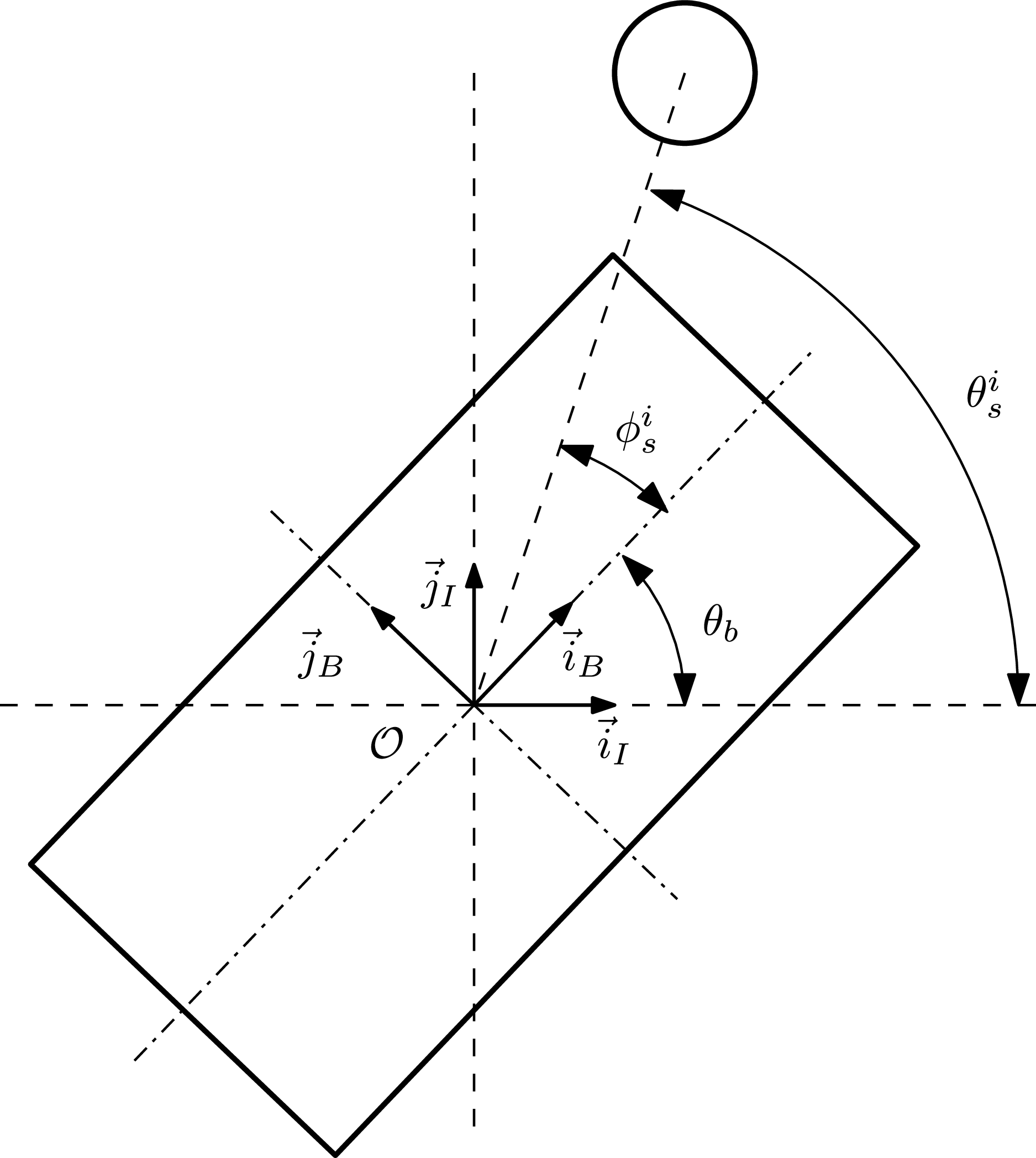
This configuration facilitates the robots’ arrangement around the object, mitigating premature collisions and setting the stage for the initiation of the pushing phase. The calculation of the caging angles is articulated as follows:
 \begin{align*} \theta _{s}^{i}&=\text{atan2}(y_{s}^{i}-y_{o},x_{s}^{i}-x_{o})\\ \phi _{s}^{i}&=\theta _{s}^{i}-\theta _{b}\text{, }i\in \{1,2,3,4\}, \end{align*}
where
 $\theta ^{i}_s$
and
 $\phi ^{i}_s$
represent the relative angles of the robots with respect to the inertial and object-fixed frames, respectively. The graphical representation of these angles is depicted in Fig. 17.
Relevant angles for the calculation of the relative angles
 $\phi ^i_{s}$
of the robots with respect to the box.

The ensuing task of pathing is to allocate the designated approach points among the four robots, considering their initial locations, with the aim of preventing collisions. Toward this end, Algorithm 4 presents the pseudocode of a sorting algorithm designed to achieve this objective. This procedure systematically assigns waypoints to each robot according to its relative orientation,
 $\phi ^{i}_{s}$
, in relation to the other robots and the object.

Let
 $\mathcal{O}:\left (\mathcal{O}_{x},\mathcal{O}_{y}\right )\in \mathbb{R}^{2}$
represent the coordinates of the box’s geometric center, and let
 $\mathcal{L}^{i}:\left (\mathcal{L}^{i}_{x},\mathcal{L}^{i}_{y}\right )\in \mathbb{R}^{2}$
, for
 $i\in \{1,\ldots ,4\}$
, denote the coordinates of the four approach points to the box, all expressed in the inertia frame. Employing straightforward geometrical principles, the coordinates of the waypoints for approaching the box are determined as follows:
 \begin{align*} \mathcal{L}^{i}:\left (\mathcal{L}^{i}_{x};\mathcal{L}^{i}_{y}\right )&=\left [\begin{array}{c} \mathcal{O}_{x}\\ \mathcal{O}_{y} \end{array}\right ]+\left [\begin{array}{c} \rho _{a}\cos \left (\theta _{b}+\frac {\pi }{2}(i-1)\right )\\ \rho _{a}\sin \left (\theta _{b}+\frac {\pi }{2}(i-1)\right ) \end{array}\right ],\;i\in \{1,\ldots ,4\}. \end{align*}
The pathing waypoints
 $ \mathcal{L}^{i}$
position the robots safely along the symmetry axes of the object, at a distance
 $ \rho _{a}$
from its geometric center
 $ \mathcal{O}$
.
Translation
Upon all robots reaching their designated initial approach points, the algorithm progresses to its second phase, focusing on generating waypoints to facilitate the object’s translation by the robots.
The translation phase is bifurcated into two parts: caging and pushing. In the caging part, robots surround the box to form a cross-shaped enclosure, positioning themselves at distances
 $\rho _{L}$
and
 $\rho _{W}$
along the box’s length and width symmetry axes, respectively. The caging waypoints, during translation, are
 \begin{align*} \mathcal{N}^{i}:\left (\mathcal{N}_{x}^{i},\mathcal{N}_{y}^{i}\right ) & =\left [\begin{array}{c} \mathcal{O}_{x}\\ \mathcal{O}_{y} \end{array}\right ]+\left [\begin{array}{c} \rho _{L}\cos \left (\theta _{b}+\frac {\pi }{2}(i-1)\right )\\ \rho _{L}\sin \left (\theta _{b}+\frac {\pi }{2}(i-1)\right ) \end{array}\right ],\;\text{for }i\in \{1,3\};\\ \mathcal{N}^{i}:\left (\mathcal{N}_{x}^{i},\mathcal{N}_{y}^{i}\right ) & =\left [\begin{array}{c} \mathcal{O}_{x}\\ \mathcal{O}_{y} \end{array}\right ]+\left [\begin{array}{c} \rho _{W}\cos \left (\theta _{b}+\frac {\pi }{2}(i-1)\right )\\ \rho _{W}\sin \left (\theta _{b}+\frac {\pi }{2}(i-1)\right ) \end{array}\right ],\;\text{for }i\in \{2,4\}. \end{align*}
After the caging formation is established, the robots initiate a uniform, parallel motion, moving in unison toward the same direction, to advance the box toward its designated target location
 $\left (x_{t},y_{t}\right )$
. This movement is facilitated by waypoints generated from a consistent directional vector and the caging waypoints. Adherence to these pushing waypoints by the robots orchestrates the collective movement of the object toward its goal.
The directional vector has a magnitude
 $\rho _{M}$
and an angle
 $\theta _{M}$
, which is determined by the bearing from the object’s center to the target location, calculated as follows:
 \begin{equation} \theta _{M} = \text{atan2}(y_{o} - y_{t}, x_{o} - x_{t}). \end{equation}
The pushing waypoints, denoted as
 $\mathcal{M}^{i}$
, are derived by applying the directional vector to the corresponding caging waypoints
 $\mathcal{N}^i$
as
 \begin{equation} \mathcal{M}^{i}:\left (\mathcal{M}_{x}^{i},\mathcal{M}_{y}^{i}\right )=\left [\begin{array}{c} \mathcal{N}_{x}^{i}\\ \mathcal{N}_{y}^{i} \end{array}\right ]-\left [\begin{array}{c} \rho _{M}\cos \theta _{M}\\ \rho _{M}\sin \theta _{M} \end{array}\right ],\text{ for }i\in \{1,\ldots ,4\}. \end{equation}
The depiction of the caging and pushing waypoints, along with the characteristics (magnitude and bearing) of the directional vector that delineates the pushing waypoints, is presented in Fig. 18. The translation phase, encompassing both caging and pushing, persists until the object arrives at its target location. This condition is mathematically satisfied when the distance
 $\rho _{t}$
between the object and the target is reduced to less than a threshold value
 $\epsilon _{t}$
, which signifies the permissible distance error tolerance from the target. Once this condition is satisfied, the algorithm advances to its final phase: rotation.
Geometric configuration elements of the group object manipulation algorithm during the translation phase.

Rotation
In the rotation phase, only two robots, lying in the opposing halfplanes defined by the box’s length symmetry axis, participate in the object manipulation process, while the other two step back and track the box’s orientation.
Assume that indexed units 2 and 4 are designated to the “long” sides of the box; they will be responsible for rotating the box. In this case, robots 1 and 3 do not participate in the manipulation process and observe the proceedings by adhering to the approaching waypoints
 $\mathcal{L}^1$
and
 $\mathcal{L}^3$
.
The “wrenching” robots – 2 and 4 – are assigned waypoints,
 $\mathcal{W}^{2}$
and
 $\mathcal{W}^{4}$
, located within the box’s footprint (see Fig. 19). The waypoints are arranged along a line segment angularly displaced from the box’s length symmetry axis by an angle
 $\theta _r$
, with their distance from the box’s center denoted by
 $\rho _{r}$
. To simplify,
 $\mathcal{W}^{2}$
and
 $\mathcal{W}^{4}$
are positioned on one of the box’s diagonals. As a result,
 $\theta _{r}$
takes on values of either
 $-\pi /4$
or
 $\pi /4$
, while
 $\rho _{r}$
must remain below half the length of the main diagonal. This arrangement ensures that, as the robots follow these waypoints, their movement will enable a rotation aimed at minimizing the box’s orientation error.
Waypoint generation in the rotation phase. Two of the robots, 2 and 4, execute the box’s turning maneuver, whereas robots 1 and 3 retract to a “spectator” configuration, following the box’s manipulation. The wrenching waypoints lie within the area of the box.

The procedure of this phase involves comparing the angular error between the box’s current orientation and its target orientation represented by the difference
 $\theta _b - \theta _t$
. The sign of this error determines whether the box will be turned clockwise or counterclockwise. If it is positive, the offset angle
 $\theta _r$
is set to
 $\pi /4$
, inducing a clockwise rotation of the box. Conversely, if the angular error is negative,
 $\theta _r$
is set to
 $-\pi /4$
, resulting in a counterclockwise rotation of the box. The waypoints that enable the rotation are expressed as follows:
 \begin{align}&\,\, \mathcal{W}^{2}:\left (\mathcal{W}^{1}_{x},\mathcal{W}^{1}_{y}\right ) =\left [\begin{array}{c} \mathcal{O}_{x}\\ \mathcal{O}_{y} \end{array}\right ]+\left [\begin{array}{c} \rho _{r}\cos\theta _{r}\\ \rho _{r}\sin\theta _{r} \end{array}\right ] \end{align}
 \begin{align}& \mathcal{W}^{4}:\left (\mathcal{W}^{4}_{x},\mathcal{W}^{4}_{y}\right ) =\left [\begin{array}{c} \mathcal{O}_{x}\\ \mathcal{O}_{y} \end{array}\right ]+\left [\begin{array}{c} -\rho _{r}\cos\theta _{r}\\ -\rho _{r}\sin\theta _{r} \end{array}\right ] \end{align}
The waypoints are employed until the object achieves the desired angular orientation, specifically when the absolute angular error
 $|\theta _{b}-\theta _{t}|$
falls below a predetermined threshold
 $\epsilon _{r}$
. Should there remain a positional error following the rotation phase, the process iteratively cycles through the translation and rotation phases until errors in both phases are reduced to within their respective predefined tolerance thresholds.
5. Experimental validation
This section presents a comprehensive overview and detailed description of the experiments conducted to validate the Arachne System’s operation, functionality, and capabilities. Additionally, we offer several tuning guidelines and indicative coefficient values for the procedural algorithms, described in Section 4, and configuration procedures for optimizing the hardware setup.
The sequence of the algorithms tested includes set-point control, single-agent object manipulation, multi-agent object manipulation, standard collision avoidance, and infrared collision avoidance. For all experiments, raw video data were captured by an overhead camera with a
 $320 \times 240$
pixel resolution and analyzed at a high frequency of
 $100\,{\textrm{Hz}}$
using Roborealm computer vision software. The processed video stream by Roboreal furnished the real-time coordinates of the Arachne Bots, which is essential for the execution of the majority of the task fulfillment algorithms. The unit of measurement for distance provided by RoboRealm is expressed in pixels. The camera’s height affects the area represented by each pixel, thereby influencing the apparent size of objects in pixels captured in the video feed.
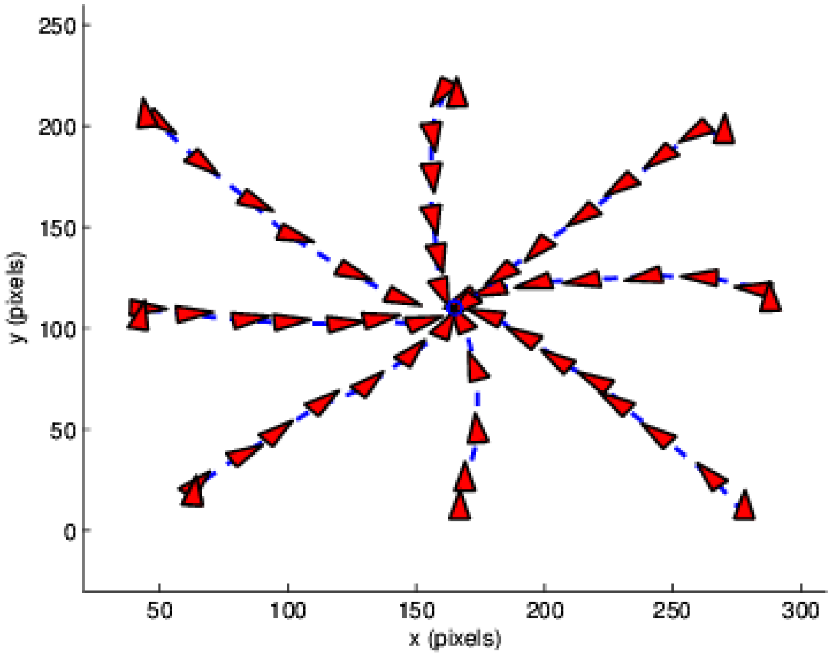
In evaluating the set-point control logic, described in Section 4.2, Arachne Bots were positioned at various starting points within the overhead camera’s field of view. For each test, the Arachne Bot initiated its movement from locations within the inner boundary of a circle, assigned to reach the exact target location positioned at the circle’s center. For this experiment, the starting positions were strategically chosen so that, for some of them, the target was positioned behind and to the aft of the robot. Figure 20 depicts a bot’s posture at periodic time instances during multiple attempts of the set-point approaching assignment. This visualization underscores the Arachne Bots’ adeptness in achieving concurrent advancement and rotation, a capability their unique walking mechanism facilitates. This functionality enables the bots to execute the fundamental operation of moving toward reference points in a configurable and efficient manner.
Set-point reaching operation: an Arachne Bot was launched from different starting positions to converge on a predetermined target location. The feedback control law incorporates the Line of Sight (LOS) criterion, under which the robot performs a pure rotation until the target enters its LOS. Upon this condition being met, the robot progresses toward the target guided by the feedback law specified in (7).

The disk radius
 $R_{t}$
, asserting that the target has been reached and illustrated in Fig. 12, was fixed at
 $15\,{\textrm{pixels}}$
. This radius is determined through empirical observation. The control logic includes the forward motion stipulation, as detailed in the pseudocode of Algorithm 1, which allows advancement towards the target only when it falls within the robot’s LOS. The angular field of view
 $\sigma$
, defining the extent of the LOS, was configured to
 $0.9\,{\textrm{rad}}$
(
 $51.6^\circ$
). A larger
 $\sigma$
angle results in a more curved trajectory. The two positive feedback gains,
 $K_{\rho }$
and
 $K_{\alpha }$
, as specified in Eq. (7), are calibrated to ensure that the static mappings from velocities to voltages yield appropriate pulse width modulation (PWM) signals for actuating the motors of the legs and torso, respectively. In the case of our Arachne Bots, both gains were set at
 $127$
. Increasing the values of these gains results in a corresponding increase in the robot’s rotational and translational speed.
Figure 20 depicts a bot’s posture at periodic time instances during multiple attempts of the set-point approaching assignment. This visualization underscores the Arachne Bots’ adeptness in achieving concurrent advancement and rotation, a capability their unique walking mechanism facilitates. This functionality enables the Arachne Bots to execute the fundamental operation of moving toward reference points configurable and efficiently. The subsequent algorithms evaluated are developed to create waypoints that, when adhered to, achieve specific objectives, such as object manipulation or collision avoidance. Positioned within the lower tier of the control system hierarchy, the set-point control logic is tasked with producing the linear and angular velocities required to reach the waypoints established by the “high-level” algorithm.
The next algorithm tested was the object manipulation task by a single Arachne Bot, explained in Section 4.4. The waypoint generation process for this task is outlined in Algorithm 3. For the object, we chose a plastic cylindrical hull with dimensions (height and radius) comparable to those of the Arachne Bot.
The radius of the object was experimentally evaluated to be approximately
 $35\,{\textrm{pixels}}$
. The distance
 $\mu _{o}$
to the contact point is set equal to the object radius. An approximation of the robot’s diameter is required to calculate certain waypoints within the algorithm, which was measured to be approximately
 $40\,{\textrm{pixels}}$
. The distance
 $\mu _{I}$
, critical for defining the approach waypoints
 $\mathcal{A}$
,
 $\mathcal{B}$
, and
 $\mathcal{I}$
, is assigned based on the combined radius of the robot and the object, totaling
 $75\,{\textrm{pixels}}$
. The tolerance threshold,
 $\epsilon _{t}$
, was fixed at
 $25\,{\textrm{pixels}}$
.
Figure 21 demonstrates the experimental implementation of the single-bot object manipulation task. The actual and target coordinates of the object (from a distinct experimental trial) over time are depicted in Fig. 22. Despite the irregular shape of its legs interacting with the round object, the Arachne Bot successfully maneuvered the object.
Single-bot object manipulation: posture of the arachne bot and object location at intermittent time points during an experimental trial. The dashed circle marks the target location area.

The object’s coordinates over time (black solid line) and its target location (dashed blue line).

The next algorithmic procedure that was validated is the box manipulation by a group of four Arachne Bots, described in Subsection 4.5. For brevity, in the subsequent description, it is implied that the index
 $i$
takes values from the set
 $\{1,2,3,4\}$
. In our experiment, the dimensions of the box were
 $(114\,{\textrm{pixels}})\times (104\,{\textrm{pixels}})$
. In our convention, we assume the box’s length to be its larger dimension.
Initially, the distances
 $\rho _{L}$
and
 $\rho _{W}$
, which determine the caging waypoints
 $\mathcal{N}^{i}$
in the translation phase, are set to be equal to half the box’s length and width, respectively, subtracting the robot’s radius. For the current setup,
 $\rho _{L}$
and
 $\rho _{W}$
were established at
 $94\,{\textrm{pixels}}$
and
 $84\,{\textrm{pixels}}$
. This fitting is essential for the bots to surround the box effectively.
Reverting to the pathing phase, the distance
 $\rho _{a}$
, defining the approach waypoints, should exceed the greater of
 $\rho _{L}$
or
 $\rho _{W}$
. In our experiments,
 $\rho _{a}$
was set to
 $1.5\rho _{L}$
, approximately
 $56\,{\textrm{pixels}}$
. For devising the pushing waypoints
 $\mathcal{W}^{i}$
, a directional vector in polar form,
 $\rho _{M}\angle \theta _{M}$
, is appended to
 $\mathcal{N}^{i}$
. This vector is intended to position the waypoints within the box for the bots executing the push, avoiding too small values that might hinder the box’s forward movement by the leading bots or too large values placing waypoints outside the box. Considering the box’s dimensions,
 $\rho _{M}$
was adjusted to
 $22\,{\textrm{pixels}}$
. The same value assigned to
 $\rho _{M}$
was also used for
 $\rho _{r}$
, denoting the distance that establishes the waypoints for the propelling bots responsible for inducing the box’s rotation. The rationale was analogous: the waypoints for the wrenching bots must be within the box. Finally, the tolerance thresholds that mark the completion of the translation and rotation phases,
 $\epsilon _{t}$
and
 $\epsilon _{r}$
, were set at
 $25$
pixels and
 $10^{\circ }$
(approximately
 $0.174$
radians), respectively.
Figure 23 illustrates nine execution snapshots acquired from data collected during an experimental trial. The execution time instance corresponding to each view is carefully chosen to ensure that the figure’s gallery comprehensively showcases all phases of the group box manipulation task. The procedure systematically and reliably leads to the successful transportation of the box to its designated posture by the group of Arachne Bots.
Group object manipulation: each view displays the configuration of the bots and the box at selected execution time instances based on data obtained during an experimental run. The sequence of tiles is arranged to be read from top to bottom and left to right.

The final two experimental setups are dedicated to exploring collision avoidance, utilizing two different proximity sensing techniques. Both implementations adhere to the algorithmic procedure outlined in Algorithm 2. The overhead camera system captures each bot’s absolute posture (position and orientation). The key distinction between the two validation procedures lies in how the proximity between each robot and its neighboring units is detected. In the first scenario, the camera system provides this relative measurement (relative distance and bearing), whereas, in the second scenario, proximity detection is facilitated by the IRB, as detailed in Section 3. The key parameter for the collision avoidance algorithm, detailed in Section 4.3, is the collision radius,
 $R_{c}$
, fixed at
 $52\, {\textrm{pixels}}$
.
Figure 24 demonstrates the trajectories and orientations of six Arachne Bots engaged in collision avoidance over successive time intervals during an experimental trial. Despite navigating in a limited space with the clutter of six Arachne Bots, the swarm members arrived at their predetermined target locations without collisions. The effectiveness of two Arachne Bots equipped with the IRB for proximity sensing during a collision avoidance algorithm trial is demonstrated in Fig. 25. Echoing the format of previous validation results, the figure captures the bots’ configurations in tiles corresponding to sequential time instances of the experiment, showcasing the IRB’s capability to provide functional sensory information for the reliable and repeated completion of the collision avoidance task. With its modest cost, compact design, and simplicity, the IRB consistently proved to be a reliable sensor for collision avoidance, reaffirming its value across multiple experimental repetitions.
Collision avoidance with the overhead camera: each tile portrays the paths and postures of six Arachne Bots at successive time instances throughout the execution of the collision avoidance algorithm in an experimental trial. The tiles are arranged to follow a viewing sequence from top to bottom and left to right.

Collision avoidance with the IRB: each tile portrays the paths and postures of two Arachne Bots at successive time instances throughout the execution of the collision avoidance algorithm in an experimental trial. Similar to the previous two illustration formats, the tiles are organized to follow a viewing sequence from top to bottom and left to right.

6. Conclusion
This work introduces a new robotics platform that is both compact and inexpensive, requiring minimal time and resources for assembly. Moreover, its simplicity makes it accessible to users who may be unfamiliar with complex robotic systems. The platform’s efficacy is evidenced by its application in testing various algorithms, including those for set-point control, single-agent object manipulation, and multi-agent object manipulation. Additionally, the platform’s design facilitates customization, as demonstrated by the integration of an IRB. The primary goal of this new platform is to propel the field of swarm robotics forward by offering an easily reproducible, low-cost, and user-friendly system. Such a system is poised to enable researchers and educational institutions alike to engage directly with collective robotic behaviors.
Acknowledgments
The authors would like to thank David J. Willis for his invaluable help in editing the paper and insightful comments for improving it. Ioannis Raptis extends his gratitude to his beloved newborn daughter, his little spider, Alexandra Rapti (born 1/28/2024), who kept him company with her coos while writing this paper. Ioannis Raptis gratefully dedicates this work to his newborn daughter, Alexandra (born 1/28/2024) – his cherished “little spider” – whose gentle coos provided comfort throughout the writing of this paper.
Author contributions
IR conceived and designed the study, wrote and edited the article, and supervised BS in developing the Arachne Bots.
Financial support
This work was partially supported by the National Science Foundation under Grant No.DGE-2105701.
Competing interests
The authors declare no conflicts of interest exist.
Ethical approval
Not applicable.