Should public retirement plans be fully funded?

HENNING BOHN

doi:10.1017/S1474747211000096

Should public retirement plans be fully funded?

Published online by Cambridge University Press: 12 April 2011

HENNING BOHN

Show author details

HENNING BOHN: Affiliation:
Department of Economics, University of California Santa Barbara, Santa Barbara, CA 93106, USA (e-mail: bohn@econ.ucsb.edu)

Article contents

Abstract
Introduction
The problem of pension funding
A model of local government
Legal ambiguity and default risk
Accounting implications of intermediation costs
Concluding comments
Footnotes
References

Rights & Permissions

Abstract

Most state and local retirement plans strive for full funding, at least by actuarial standards. Funding measured at market values fluctuates and often falls short. In a model where most taxpayers hold debt and face intermediation costs, returns on pension assets are less than taxpayers’ costs of borrowing. Hence, zero pension funding is optimal. Also, unfunded pension promises are properly discounted at a rate strictly greater than the government's borrowing rate. Funding can still be in taxpayers’ interests if legal enforcement problems make unfunded pensions risky for employees, but except in special cases, the optimal funding ratio is less than 100%.

‘Neither a borrower nor a lender be’ (Shakespeare)

Information

Type: Articles
Information: Journal of Pension Economics & Finance , Volume 10 , Issue 2 , April 2011 , pp. 195 - 219

DOI: https://doi.org/10.1017/S1474747211000096 [Opens in a new window]
Copyright: Copyright © Cambridge University Press 2011

1. Introduction

Most state and local retirement plans strive for full funding as measured by actuarial standards. Funds are commonly invested in risky assets. Hence, actual funding ratios – the ratios of assets to accrued benefit obligations – fluctuate and are often less than 100%. Press reports about underfunding naturally cause taxpayer anxiety. Recent experience follows this pattern. Although average funding ratios were over 80% before the recent financial crisis, many state and local pension funds are now seriously underfunded (Munnell et al., Reference Munnell, Haverstick, Sass and Aubry2008, Reference Munnell, Haverstick, Sass, Aubry and Quinby2010). Concerns about funding are reinforced by controversies about actuarial standards. Some economists have argued that officially reported funding ratios are inflated because pension obligations are computed at excessively high discount rates (Novy-Marx and Rauh, Reference Novy-Marx and Rauh2009).

This paper first reviews these issues broadly and then examines the implications of an observation seemingly ignored in the literature: Most U.S. voters and taxpayers are borrowers. (See Table 1 for evidence, discussed below.) If borrowers incur positive intermediation costs – or at least if marginal intermediation costs are increasing and positive at sufficiently high debt levels – there is a wedge between the market return on financial assets and the cost of borrowing.

Table 1.

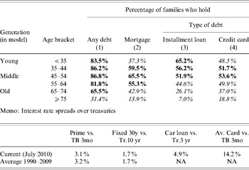
What percentages of U.S. families are borrowers?

Legend: Bold=majority. Italics=minority.

Sources: Percentage of families’ data from Survey of Consumer Finances 2007. Mortgage refers to mortgages secured by primary residence. Rate spread averages are own calculations based on FRB release H.15. Current spreads from the Wall Street Journal for 9 July 2010. Prime vs. TB 3mo=Prime rate minus 3-month Treasury bill rate. Fixed 30 y vs. Tr.10 yr=30-year fixed rate mortgage rate minus 10-year Treasury rate. Car loan vs. Tr.3 yr=Average rate on 36 month car loans minus 3-year Treasury rate (Per SCF, car loans are the most common installment loans). Av. Card vs. TB 3mo=Average rate on credit cards minus 3-month Treasury bill rate.

Positive intermediation costs have strong implications for public pension funding: Zero funding is optimal for taxpayers who hold debt. The basic argument is that indebted taxpayers are better off if, instead of paying taxes to fund public pensions that earn the market return, they leave pensions unfunded, defer the taxes until pension payouts are due, and use the funds to reduce their debt, which accumulates at a higher interest rate.

Because about 75% of U.S. families are debtors, this simple argument suggests that zero funding is optimal for a large majority of taxpayers – a strikingly negative answer to this paper's title question. To anticipate, the analysis will indeed show that there is a strong case against full funding, and a good case for zero funding as benchmark. The main challenge is to convert the simple argument at the individual (debtor) level into a result about policy in general equilibrium.

The two main complications are (1) to explain why debtors’ interests should determine public policy even though on aggregate, there is as much lending as borrowing, and many debtors also hold assets; and (2) to reconcile unfunded pensions with the balanced-budget principle, which restricts public debt and seems popular with voters.

My model explains the coexistence of borrowing and lending in part by life-cycle consumption smoothing, and in part by national tax incentives. To capture life-cycle borrowing, the model considers a local community of adults who live for three periods – young, middle, and old age. The young and middle-aged work, the old are retired. Young individuals borrow and middle-aged individuals are net savers. A tax incentive arises because marginal (national) income tax rates are generally higher in working age than in retirement. This means retirement savings have an after-tax return strictly greater than the market return. Hence, the middle-aged simultaneously borrow and hold retirement assets, provided the tax incentives exceed the borrowing costs. In equilibrium, all interested taxpayers hold debt.

Note that the same tax incentive gives middle-aged taxpayers an argument against public pension funding even if they are not debtors. They are better off if, instead of using after-tax income to fund public pensions, they save more on a pre-tax basis and pay local taxes later, out of less-taxed retirement income. Their incentives are aligned with debtors.

To reconcile unfunded pensions with restrictions on public debt, the model makes two assumptions. First, local taxes are property taxes. Future property taxes are then capitalized into house values, which dampens voter incentives to defer taxes beyond their lifetimes. Second, public debt is bounded because intermediation costs increase on the margin, at least at high levels of debt. Repeated voting then yields a finite equilibrium public debt. I show that because current voters (debtors) have discount rates greater than the market return, equilibrium debt is higher than the debt level that would maximize house values. Restrictions on public debt are then generally Pareto improving, can be sustained as sequential equilibrium in a voting game, and can be interpreted broadly as balanced-budget restrictions.

In this setting, with or without debt restrictions, voting over pensions always yields zero funding as a unique outcome – the outcome preferred by all voters over any other funding level. In summary, the simple insight that borrowers prefer zero pension funding is valid in general equilibrium.

The main model focuses on the case against funding. This is not to deny that there are arguments in favor of funding, which may explain why most public retirement plans have some funding. One important issue is legal ambiguity, which makes unfunded promises potentially unenforceable. (Uninsurable default would have similar implications.) The argument, which I present in an extension, is that if employees are risk averse and cannot insure against enforcement problems, the employer must pay a wage premium. A dedicated retirement fund that provides credible collateral then allows employers to reduce total compensation. This creates a trade-off between taxpayers’ intermediation costs (the basic argument) and reduced labor costs. The extended model yields partial funding near 100% if employees are highly risk averse and highly dependent on the pension for their retirement consumption.

The analysis has implications for pension accounting and pension regulations. First, the appropriate discount rate for unfunded Defined Benefit (DB) pensions is taxpayers’ marginal cost of funds. If most taxpayers are borrowers, the appropriate discount rate is a risk-adjusted borrowing rate, which is higher than the safe interest rate. Second, because funding is costly and full funding is usually suboptimal, regulations that impose full funding undermine employer incentives to offer DB plans. Most private employers phased out their DB plans after costly funding and insurance requirements were imposed in the 1970s. If current political anxieties about public retirement plans lead to excessive funding requirements, the effects may prove similarly destructive.

The paper is organized as follows. Section 2 reviews pension funding in general. Section 3 sets up an overlapping generations’ model with local property taxes to study pension funding. Section 4 examines the impact of legal ambiguities and default risk. Section 5 comments on accounting implications. Section 6 concludes. Proofs are given in the appendix.

2. The problem of pension funding

This section examines pension funding broadly, both to review the literature and to introduce key issues for the model. The focus is on U.S. state and local government pensions and does not consider federal programs.

To start, one must distinguish between DB and Defined Contribution (DC) plans. Whereas DC plans promise only contributions, DB plans promise a formula-determined retirement income in exchange for a reduced salary. Thus, DB promises are a form of deferred compensation and create liabilities for the employer. Funding means setting aside financial assets dedicated to making promised payments. About 80% of state and local retirement plans are DB plans (Munnell et al., Reference Munnell, Haverstick, Sass and Aubry2008).

The DB design raises several questions: What is full funding, and does it ensure that all promised payments are covered? How does deferred compensation relate to the principle of balanced budgets, and does this principle impose a norm that DB pensions should be fully funded? And what are the costs and benefits of funding?Footnote ¹

2.1. The ambiguous meaning of full funding

There are at least three different ways to interpret full funding. I will call them the accounting view, the finance view, and the populist view.

The accounting view considers a retirement plan fully funded if an actuarial measure of fund assets equals an actuarial measure of accrued liabilities. Accounting rules for U.S. state and local governments are set by the Government Accounting Standards Board (GASB). The key rule for pension accounting, GASB 25, gives plan sponsors a choice between several different actuarial methods for pension obligations (see Peng, Reference Peng2009). A common approach is to use expected returns on assets to determine the discount rate on liabilities. Measures of funding are the unfunded actuarial accrued liability (UAAL), the gap between liabilities and assets, and the funding ratio, which is the ratio of assets over liabilities. If a plan sponsor makes contributions under GASB rules, assets should equal liabilities on average, but due to capital gains and losses, the funding ratio will almost always differ from 100%. GASB rules specify that any positive or negative UAAL must be amortized over time by raising or lowering new contributions.

The finance view also considers a pension fully funded if pension assets match the present value of promised pensions (e.g., Novy-Marx and Rauh, Reference Novy-Marx and Rauh2009). In contrast to the accounting view, state-contingent claims pricing is used to value obligations, and economic rather than legal reasoning is used to ascertain the scope of obligations (Bulow, Reference Bulow1982). Because pension promises have strong legal protections (see Brown and Wilcox, Reference Brown and Wilcox2009; Peng, Reference Peng2009), the default risk is widely considered negligible. Hence, finance principles call for discounting at ‘safe’ interest rates, which are lower than the discount rates used by accountants. The resulting present values are higher. So plans that are well funded by GASB standards are often underfunded by finance standards (Novy-Marx and Rauh, Reference Novy-Marx and Rauh2009).

The analysis below will show that intermediation costs provide a rationale consistent with standard finance for discount rates greater than the safe interest rate.

By populist view, I mean the view reflected in newspaper stories that portray any occurrence of underfunding as disturbing or scandalous. This view treats a pension plan as not fully funded unless pension assets cover all future obligations in all states of nature, even under adverse conditions, so that there is no risk of a shortfall that might require employer contributions.

It may be tempting for politicians and regulators to cater to negative publicity by imposing increasingly stringent valuation standards. However, a pursuit of zero risk is probably futile, and threatens to reinforce the apparent misperception that enough funding might somehow release the sponsor from its liabilities. The analysis below will show that funding requirements generally reduce welfare.

2.2. Balanced-budget rules and deferred compensation

Almost all state and local governments operate under balanced-budget rules. A separate capital budget allows for bond financing, usually subject to voter approval, with bonds repaid out of operating funds. Pension funds are commonly separate entities, funded by contributions from the operating budget and dedicated to paying retirees.

Underfunded public pensions complicate this fiscal framework. A funding shortfall due to unexpectedly low investment returns reduces government net worth. A shortfall because of missed contributions means that the operating budget understates employee compensation. Hence, one must ask if the balanced-budget principle demands full funding, or otherwise constrains funding. The question is important because according to opinion polls, balanced budgets are extremely popular.Footnote ²

The literature on balanced budgets unfortunately does not provide clear answers. A theoretical literature on national debt has identified political distortions that tend to favor excessive debt (see, e.g., Alesina and Perotti, Reference Alesina and Perotti1995; Persson and Tabellini, Reference Persson and Tabellini2000). For example, uncertainty about re-election may shorten politicians’ planning horizons and invite the use of debt as a tool to constrain successor governments. A fiscal rule imposing balanced budgets is a natural corrective mechanism for such distortions.

There may also be simple principal–agent explanations of why voters like balanced budgets. Voters must monitor politicians who act as their agents. Credible information about local budgets is often unavailable or costly. The potential damages from political favoritism, corruption, or other monitoring failures are much greater if politicians can incur debt than if expenditures are bounded by current revenues.Footnote ³

These arguments about balanced budgets do not directly address public pensions and their funding. One may argue by analogy that the distortions that favor excessive debt also favor borrowing through underfunded pensions. Then funding requirements complement a balanced-budget rule. If corruption is a concern, however, funding rules that place vast pools of financial assets under the control of politicians may be quite dangerous. Monitoring the performance of investment managers is difficult, especially if they have authority to invest in risky assets, and so incompetence or fraud can be disguised as bad luck. Recurrent scandals involving ‘pay to play’ schemes suggest that monitoring is a problem. The problem would be eliminated if public pensions were left unfunded.

The analysis below treats the popularity of balanced budgets as a stylized fact that economic theory should explain or at least respect. The question how pension funding should be treated within a balanced-budget framework is addressed as part of the analysis.

Note that there is a literature on state and local pensions without balanced budgets. D'Arcy et al. (Reference D'Arcy, Dulebohn and Oh1999) argue that with distortionary taxes, optimal pension funding should be governed by tax smoothing arguments. They conclude that a range of funding levels can be optimal, depending on the growth rates of taxes and expenditures. Lucas and Zeldes (Reference Lucas and Zeldes2009) note that pension funding and investment strategy would be irrelevant if Ricardian neutrality applied; they also examine ramifications of tax smoothing. Bader and Gold (Reference Bader and Gold2007) examine tax arbitrage opportunities in public pensions. The analysis here differs from this literature by accepting the popularity of balanced budgets.

2.3. Pension returns and taxpayers’ cost of funds

The financial situation of taxpayers has received remarkably little attention in the pension literature. Because state and local taxpayers are the ultimate sponsors of public retirement plans, their opportunity costs of funds should matter for determining optimal funding levels. For taxpayers, the decision on how to fund their government's public retirement plan is fundamentally a choice to pay taxes when pension promises are made or to defer taxes until the promised pensions are due.

The implicit assumption in the literature seems to be that taxpayers are savers who have essentially the same investment opportunities as the government (e.g., Lucas and Zeldes, Reference Lucas and Zeldes2009). Hence, pension funding has zero opportunity cost. For borrowers, however, paying taxes to fund public pensions is costly, because loan rates include charges for intermediation costs – the costs of screening, monitoring, and other administrative expenses. Hence, loan rates are generally higher than the returns available on investments.

Table 1 documents the prevalence of debt among U.S. families. According to the Survey of Consumer Finances 2007 (SCF), more than 80% of families with heads of household under 65 hold debt. Retirees are somewhat less indebted. Credit card debt is held by majorities in the 35–54 age brackets, installment debt by majorities in the under-54 age brackets, and mortgages by majorities in the 35–64 age brackets. Thus, most U.S. families hold debt, including the vast majority of working-age families.

Table 1 also shows how interest rates on popular types of loans compare with Treasury rates. Spreads between T-bills and credit card rates are about 14%, spreads on car loans (the most common installment loan) are about 5%, and spreads on prime mortgages are about 1.7%. The interpretation is difficult because these spreads include compensation for default risk in addition to intermediation costs. A further complication is that if borrowers rationally move from low-cost to higher-cost loans as their debt increases, average interest spreads understate the marginal costs of borrowing. In theory, a risk-adjustment of investment returns should yield the safe interest rate as risk-adjusted return, and a risk-adjustment of loan rates should yield the safe interest rate plus intermediation costs. A useful benchmark is the spread between the Prime rate and the T-bill rate, which is about 3%. Because prime loans are granted only to the best borrowers, the Prime spread is reasonable proxy for intermediation costs. This suggests that intermediation costs are a significant opportunity cost for borrowers.Footnote ⁴

Because most families are in debt, the preferences of borrowers deserve attention in thinking about optimal public policy. A possible counterargument is that many borrowers also hold financial assets, notably retirement savings. In addition, one may wonder if a focus on borrowing is incomplete because aggregate net worth is positive – which means borrowing is less than saving – and because some borrowing is encouraged by tax incentives. To address these complications, the next section presents a model that includes debt subject to intermediation costs, retirement saving, and saving incentives.

3. A model of local government

This section examines a model of local public pensions. The model considers a community with overlapping generations of tax-paying residents/voters. The local government hires public employees to produce public services that are financed by property taxes. Public debt and public pensions are capitalized into home prices, as in Epple and Schipper (Reference Epple and Schipper1981).Footnote ⁵ To keep the model tractable, I reduce the life cycle to three periods and abstract from uncertainty.

3.1. Assumptions and a benchmark allocation

The community is populated by overlapping generations of individuals (adults) who live for three periods – young, middle, and old age. Time is indexed by t and cohorts by age i (i=1, 2, 3). The community has an exogenous number of residents (Nⁱ) in each cohort. The young supply one unit of labor and earn a wage w. The middle-aged supply e>1 units of labor and earn ew. The old do not work and may receive transfers TR from the national government. All individuals have preferences over consumption (c_tⁱ), local public services (g_t), and housing.

The wage w and the interest rate r are constant and are determined outside the community.Footnote ⁶ Also assume perfect foresight about future government policy and no defaults on debt, so all optimization problems are deterministic.

Assume that the community has $\bar{N}$ houses that can be owned by residents or by commercial owners. Owner-occupied houses provide a consumption value v(g_t) per period for the young and middle-aged, which depend on public services, and assume v(⋅) is increasing and concave. Utility of individuals born in generation t is

(1)

$U_{t} \equals u\lpar c_{t}^{\setnum{1}} \plus h_{t}^{\setnum{1}} v\lpar g_{t} \rpar \rpar \plus \beta u\lpar c_{t \plus \setnum{1}}^{\setnum{2}} \plus h_{t \plus \setnum{1}}^{\setnum{2}} v\lpar g_{t \plus \setnum{1}} \rpar \rpar \plus \beta ^{\setnum{2}} u\lpar c_{t \plus \setnum{2}}^{\setnum{3}} \rpar \comma$

where β∊(0,1) captures time preference, h_tⁱ∊[0,1] indicates home ownership, and u(⋅) is increasing and strictly concave. (Ownership greater than one is treated as commercial.) Homeowners pay property taxes T_t.

Commercial owners earn the value v(g_t) as rental income per house, but unlike residents, they incur a management cost χ_H>0.Footnote ⁷ Thus, rental income is v(g_t)−T_t−χ_H. Assume $\bar{N} \gt N^{\setnum{1}} \plus N^{\setnum{2}}$ (there are more houses than residential buyers), so house prices are determined by commercial owners. They capitalize rental income at rate r, which yields a house price

(2)

$H_{t} \equals \mathop {\sum}\limits_{n \equals \setnum{0}}^{\infty } {\left( {{1 \over {1 \minus r}}} \right)^{n} } \lpar v\lpar g_{t \plus n} \rpar \minus T_{t \plus n} \minus \chi _{\rm H} \rpar.$

Public services are produced by local government employees. Let production with L _t¹ young and L _t² middle-aged public employees be

(3)

$g_{t} \equals G\lpar L_{t}^{\setnum{1}} \sol \bar{N}\comma L_{t}^{\setnum{2}} \sol \bar{N}\rpar \comma$

where G is increasing, concave, and has constant returns to scale.

As simple benchmark, suppose the government pays non-deferred market wages, balances its budget, and maximizes house prices. Then labor costs are wL _t¹+ewL _t² and property taxes are $T_{t} \equals \lpar wL_{t}^{\setnum{1}} \plus ewL_{t}^{\setnum{2}} \rpar \sol \bar{N}$ per house. Cost minimization requires G ₂(l,1−l)/G ₁(l,1−l)=e, which defines an optimal share of young workers l=L ¹/(L ¹+L ²) and a unit cost T_t/g_t=w[l+e(1−l)/G(l,1−l)]≡χ_g. The optimality condition v′(g_t)=χ_g defines optimal public services g*=(v′)⁻ ¹(χ_g) and optimal employment $L^{\setnum{1}\ast } \equiv l \cdot \bar{N}g{\ast } \sol G\lpar l\comma 1 \minus l\rpar$ and $L^{\setnum{2}\ast } \equiv \lpar 1 \minus l\rpar \bar{N}g{\ast } \sol G\lpar l\comma 1 \minus l\rpar$ . The implied house price is

(4)

$H{\ast } \equals \mathop {\sum}\limits_{n\geqslant \setnum{0}} {\left( {{1 \over {1 \plus r}}} \right)^{n} \lsqb v\lpar g{\ast } \rpar \minus \chi _{g} g{\ast } \minus \chi _{\rm H} \rsqb } \equals {{\lpar 1 \plus r\rpar } \over r}\lsqb v\lpar g{\ast } \rpar \minus \chi _{g} g{\ast } \minus \chi _{\rm H} \rsqb.$

Assume χ_H<v(g*)−χ_gg* to ensure a positive house price.

A key assumption is that borrowers must incur intermediation costs, for example, screening and monitoring costs. Intermediation costs may differ by type and amount of debt, and there may be tax benefits for home mortgages. To express the menu of borrowing choices parsimoniously, assume borrowers rank alternative sources of debt by net borrowing costs, which means intermediation costs minus tax benefits. Let χ_dⁱ(d) denote the resulting schedule of marginal costs, let $\bar{\chi }_{d}^{i} \lpar d\rpar \equals {\textstyle{1 \over d}}\int_{\setnum{0}}^{d} {\chi _{d}^{i} \lpar x\rpar } x\,{\rm d}x$ be the average cost of debt d, and let $1 \plus \bar{r}_{d}^{i} \lpar d\rpar \equals \lpar 1 \plus r\rpar \lpar 1 \plus \bar{\chi }_{d}^{i} \lpar d\rpar \rpar$ be the promised repayment in period t+1. Assume borrowing costs depend at most on age and on homeownership (h_tⁱH_t), and assume:

Assumption 1. Marginal intermediation costs χ_dⁱ are strictly increasing and continuous with χ_dⁱ→∞ as d→∞ and χ_dⁱ(hⁱH)>0.

For homeowners, this allows χ_dⁱ(0)<0, which means intermediation would be negative up to ${\tilde d}\vskip-.2pt \hskip1pt^{i} \equiv \lpar \chi _{d}^{i} \rpar ^{ \minus \setnum{1}} \lpar 0\rpar$ <hⁱH. The essence of Assumption 1 is therefore that marginal costs exceed tax benefits as the loan-to-value ratio approaches 100%, and that other debt is costly. The intermediation costs have to be sufficiently strong to outweigh the federal tax subsidy. Define (χ_dⁱ)⁻ ¹(x)=0 for all x⩽χ_dⁱ(0); so (χ_dⁱ)⁻ ¹ and $\tilde{d}\vskip-.2pt \hskip1pt^{i} \equiv \lpar \chi _{d}^{i} \rpar ^{ \minus \setnum{1}} \lpar 0\rpar$ are always defined. I will refer to debt $d_{t}^{i} \gt \tilde{d}\vskip-.2pt \hskip1pt^{i}$ as costly debt.

Income taxes are a key motivation for saving in retirement plans. To model taxes, assume the national government taxes income at constant rates τⁱ that are age specific. The motivation is that U.S. income taxes are progressive and the age-earnings profile peaks in middle age, which means marginal tax rates tend to peak in middle age. Age-specific tax rates are a simple way to capture these stylized facts (without modeling progressivity). Assume specifically:

Assumption 2. Taxes peak in middle age: τ²>τ³⩾0 and τ²⩾τ¹>0.

This means tax rates are highest in middle age, strictly positive in working age, and strictly less in retirement than during peak earnings years. Income taxes apply to wage income minus pension contributions, to returns on regular (taxable) investments, and to pension payouts.

With income taxes, employers have an incentive to offer retirement plans.Footnote ⁸ In this deterministic setting, assets in DB and DC plans earn a market return equal to r. The only difference is that DB plans give employers a choice of funding, whereas DC plans are always funded. Assuming employers compete for workers, all tax savings accrue to workers, and employer contributions reduce cash wages one-for-one. If private employers’ cost of capital is r, they have no reason to defer funding. Hence, one may assume that private employers offer DC plans and let employees make (and choose) the contributions.

The after-tax return on retirement saving at age i can be written as

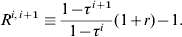
$R^{i\comma i \plus \setnum{1}} \equiv {{1 \minus \tau ^{i \plus \setnum{1}} } \over {1 \minus \tau ^{i} }}\lpar 1 \plus r\rpar \minus 1.$

This is because one unit of after-tax income at age i requires 1/(1−τⁱ) units of pre-tax income that can be saved instead; the saving earns interest r; and the accumulated assets are taxed at rate τⁱ ⁺¹.Footnote ⁹Assumption 1 implies R ²³>r and R ¹²⩽r, and so retirement contributions are encouraged in middle age and discouraged in young age.

Individuals must then account separately for taxable savings, pension savings, and debt. Let x_tⁱ⩾0 denote DC retirement contributions (for i=1, 2) and let

(5)

$X_{t \plus \setnum{2}} \equals x_{t}^{\setnum{1}} \lpar 1 \plus r\rpar ^{\setnum{2}} \plus x_{t \plus \setnum{1}}^{\setnum{2}} \lpar 1 \plus r\rpar$

denote retirement income (pre-tax). Let a_tⁱ⩾0 denote taxable assets at the end of a period, and let d_tⁱ⩾0 denote debt. The individual budget equations are:

(6)

$c_{t}^{\setnum{1}} \plus h_{t}^{\setnum{1}} \lpar H_{t} \plus T_{t} \rpar \equals \lpar w \minus x_{t}^{\setnum{1}} \rpar \lpar 1 \minus \tau ^{\setnum{1}} \rpar \plus d_{t}^{\setnum{1}} \minus a_{t}^{\setnum{1}} \comma$

which says the young finance consumption, home purchases, and property taxes from after-tax wages and net borrowing;

(7)

$\eqalign{ c_{t \plus \setnum{1}}^{\setnum{2}} \plus h_{t \plus \setnum{1}}^{\setnum{2}} T_{t \plus \setnum{1}} \plus \lpar h_{t \plus \setnum{1}}^{\setnum{2}} \minus h_{t}^{\setnum{1}} \rpar H_{t \plus \setnum{1}} \equals \tab \lpar ew \minus x_{t \plus \setnum{1}}^{\setnum{2}} \rpar \lpar 1 \minus \tau ^{\setnum{2}} \rpar \plus d_{t \plus \setnum{1}}^{\setnum{2}} \minus a_{t \plus \setnum{1}}^{\setnum{2}} \cr \tab \plus \lsqb 1 \plus r\lpar 1 \minus \tau ^{\setnum{2}} \rpar \rsqb a_{t}^{\setnum{1}} \minus \lpar 1 \plus r\rpar \lpar 1 \plus \bar{\chi }\lpar d_{t}^{\setnum{1}} \rpar \rpar d_{t}^{\setnum{1}} \comma \cr}$

so the middle-aged finance consumption, property taxes, and changes in home ownership from after-tax wages and changes in net borrowings; and

(8)

$c_{t \plus \setnum{2}}^{\setnum{3}} \equals \lpar 1 \minus \tau ^{\setnum{3}} \rpar X_{t \plus \setnum{2}} \plus TR_{t \plus \setnum{2}} \plus h_{t \plus \setnum{1}}^{\setnum{2}} H_{t \plus \setnum{2}} \minus \lpar 1 \plus r\rpar \lpar 1 \plus \bar{\chi }\lpar d_{t \plus \setnum{1}}^{\setnum{2}} \rpar \rpar d_{t \plus \setnum{1}}^{\setnum{2}} \plus \lsqb 1 \plus r\lpar 1 \minus \tau ^{\setnum{3}} \rpar \rsqb a_{t \plus \setnum{1}}^{\setnum{2}}.$

which means the old consume their retirement income and housing wealth minus net debt.

In general, the individual problem of maximizing utility by choice of assets (a_t ¹,a_t ₊₁²), debt (d_t ¹,d_t ₊₁²), retirement contributions (x_t ¹,x_t ₊₁²), and home ownership (h_t ¹,h_t ₊₁²) involves a multitude of Kuhn–Tucker constraints that may or may not bind, reflecting a range of possibly optimal borrowing and saving strategies. To avoid distracting case distinctions, assume all residents buy homes, the young want to consume more than they earn, and a home price is not enough to finance retirement. That is:

Assumption 3 Model parameters are such that individuals optimally choose h_t ¹=h_t ₊₁²=1, c_t ¹>w_t, and c_t ₊₂³>H_t ₊₂+TR_t ₊₂.

Intuitively, home ownership is optimal if χ_H is sufficiently high. Borrowing in young age is optimal if β is sufficiently low and saving for retirement is optimal if house prices and transfers are not too high.Footnote ¹⁰

These assumptions suffice to characterize the marginal rates of substitution between periods. Define

${\rm MRS}_{t}^{\setnum{12}} \equiv {{u'\lpar \hskip1.5pt \hat{c}_{t}^{\setnum{1}} \rpar } \over {\beta u'\lpar \hskip1.5pt \hat{c}_{t \plus \setnum{1}}^{\setnum{2}} \rpar }}\quad {\rm and}\quad {\rm MRS}_{t \plus \setnum{1}}^{\setnum{23}} \equiv {{u'\lpar \hskip1.5pt \hat{c}_{t \plus \setnum{1}}^{\setnum{2}} \rpar } \over {\beta u'\lpar \hskip-0.5pt c_{t \plus \setnum{2}}^{\setnum{3}} \rpar }}\comma$

where $\hat{c}_{t}^{i} \equals c_{t}^{i} \plus v\lpar g_{t} \rpar$ . Then one obtains (see the appendix for all proofs):

Proposition 1 Under Assumptions 1–3:

(a) The young incur costly debt, $d_{t}^{\setnum{1}\ast } \gt \tilde{d}$ , and they do not save (x_t ^1*=a_t ^1*=0).
(b) The middle cohort makes retirement contributions x_t ₊₁^2*>0.
(c) Both cohorts have marginal rates of substitution greater than the market interest rate:
(9)
${\rm MRS}_{t}^{\setnum{12}} \equals \lpar 1 \plus \chi _{d} \lpar d_{t}^{\setnum{1}} \rpar \rpar \lpar 1 \plus r\rpar \gt 1 \plus r\quad {\rm and}\quad {\rm MRS}_{t \plus \setnum{1}}^{\setnum{23}} \equals \lpar 1 \plus r\rpar \lpar 1 \plus R^{\setnum{23}} \rpar \gt 1 \plus r.$
(d) The middle cohort borrows d_t ₊₁^2*=(χ_d ²)⁻ ¹(R ²³) and has no taxable saving (a_t ₊₁^2*=0).

The key point of Proposition 1 is that both cohorts have marginal rates of substitution strictly greater than 1+r. This provides a setting for local government policy where young and middle-aged voters have strong incentives to defer property taxes.

Assume that voting over policy takes place every period after the housing market clears. The old are then indifferent about property taxes and can be assumed to abstain. Hence, in this model, all voters with an interest in public policy are borrowers. In the following, to avoid reiterating that the old are indifferent, let ‘voters’ refer to those who are not indifferent, i.e., usually the young and middle aged.

Several model properties are worth noting. First, one can show that without Assumption 3, MRS²³⩾(1+r)(1+R ²³) always holds, so R ²³>r alone would be sufficient for MRS²³>1+r. Second, d_t ₊₁^2*>0 holds if and only if χ_d ²(0)<R ²³. To avoid case distinctions, assume χ_d ²(0)<R ²³ in the following, and so the middle-aged hold non-zero debt. (From Table 1, this is the empirically relevant case.) Then MRS_t ₊₁²³=(1+χ₂²(d_t ₊₁^2*))(1+r), and so the Euler equations for young and middle cohorts can be written generically as MRS=(1+χ_d(d))(1+r). Third, if the national tax system were changed to eliminate borrowing incentives in middle age (e.g., if τ¹=τ²=τ³>0), middle-aged voters would become indifferent about tax payments that are invested in the market. However, young voters’ discount rates would still exceed the market rate r, and their incentives to defer taxes would not encounter opposition. Hence, all interested voters would still be borrowers. Fourth, the model implies that the young should not contribute to pensions. Many young families in the U.S. indeed contribute almost nothing, which is sometimes considered puzzling. According to SCF, 58% of families under 35 have no retirement accounts at all. Hence, zero contributions are a useful benchmark. Finally, note that despite all the borrowing, aggregate net wealth in this community can be positive, namely if retirement assets plus housing wealth exceed the debts.

The model is silent about financial flows within a period. Since every retiree has incentives to take a reverse mortgage, one may interpret this model as an economy where everyone holds debt – from early adulthood until the day of death. This suggests that if one subdivided the life cycle into more than three periods, retirees would have voting interests like the middle-aged in this model and be indifferent only in their final period of life.

For interpreting empirical data, risk and the distinction between risk premiums and intermediation costs are important. Note therefore that the analysis here generalizes straightforwardly to a stochastic setting with risky asset returns and defaultable debt. If the exogenous interest rate r is replaced by an exogenous pricing kernel for state-contingent claims, marginal rates of substitution differ from the pricing kernel by the same factors 1+χ_d(d_t ^1*) and 1+χ₂²(d_t ₊₁^2*)=1+R ²³ as in the deterministic model (see Bohn, Reference Bohn2010). Because the economic forces here – borrowing costs and tax incentives – are not stochastic, abstracting from uncertainty is without loss of generality.

As rough calibration of tax incentives, suppose tax rates for the middle-aged decline from τ²=30% to τ³=15% over a period of about 20 years. Then (1−τ²)/(1−τ³)=0.85/0.70=(1+0.98%)²⁰, and so R ²³ provides an extra return of about 1% annually. Recall from the discussion of interest rates (Section 2.3, Table 1) that intermediation costs on consumer debt are about 3% (using the Prime rate spread as proxy). This suggests that retirement savers hold only debt with relatively low intermediation costs (e.g. mortgages). It also suggests that the marginal rate of substitution of the young is greater than – and further away from the market return – than the marginal rate of substitution of the middle aged. Next consider voting.

3.2. Voting over policy: intuition

Every period, the local government must make several operational and financing decisions. The operational choices are about public services (g_t), number of young and middle-aged employees (L_t ¹,L_t ²), and about their compensation plan (DB or DC). The financing decisions are about public debt and the funding of pension promises.

A simple marginal argument provides useful intuition to guide the analysis. Voters care about policy because their utility depends on property taxes, public services, and the house value when they are old. Consider the present value of these items discounted using the voter's own marginal rate of substitution. For middle-aged voters, this means

$V_{t}^{\setnum{2}} \equiv \lpar v\lpar g_{t} \rpar \minus T_{t} \rpar \plus {1 \over {{\rm MRS}_{t}^{\setnum{23}} }}H_{t \plus \setnum{1}} \comma$

because period-t middle-aged value period-t taxes and public services, and they sell their house in period t+1. The young value taxes and public services in periods t and t+1, and they sell their house in period t+2, so

$V_{t}^{\setnum{1}} \equiv \lpar v\lpar g_{t} \rpar \minus T_{t} \rpar \plus {1 \over {{\rm MRS}_{t}^{\setnum{12}} }}\left[ {\lpar v\lpar g_{t \plus \setnum{1}} \rpar \minus T_{t \plus \setnum{1}} \rpar \plus {1 \over {{\rm MRS}_{t \plus \setnum{1}}^{\setnum{23}} }}H_{t \plus \setnum{2}} } \right].$

Using (2) and (9), these values can be written as

(10)

$V_{t}^{\setnum{2}} \equals \lpar v\lpar g_{t} \rpar \minus T_{t} \rpar \plus {1 \over {1 \plus \chi _{d} \lpar d_{t}^{\setnum{2}\ast } \rpar }}\mathop{\sum}\limits_{n\geqslant \setnum{1}} {\left( {{1 \over {1 \plus r}}} \right)^{n} } \left( {v\lpar g_{t \plus n} \rpar \minus T_{t \plus n} \minus \chi _{\rm H} } \right)$

and

(11)

$\eqalign{V_{t}^{\setnum{1}} \equals \tab \lpar v\lpar g_{t} \rpar \minus T_{t} \rpar \plus {1 \over {1 \plus \chi _{d} \lpar d_{t}^{\setnum{1}\ast } \rpar }}{{v\lpar g_{t \plus \setnum{1}} \rpar \minus T_{t \plus \setnum{1}} } \over {\lpar 1 \plus r\rpar }} \cr \tab\plus {1 \over {\lpar 1 \plus \chi _{d} \lpar d_{t}^{\setnum{1}\ast } \rpar \rpar \lpar 1 \plus \chi _{d} \lpar d_{t \plus \setnum{1}}^{\setnum{2}\ast } \rpar \rpar }}\mathop{\sum}\limits_{n\geqslant\setnum{2}} {\left( {{1 \over {1 \plus r}}} \right)^{n} } \left( {v\lpar g_{t \plus n} \rpar \minus T_{t \plus n} \minus \chi _{\rm H} } \right).}$

It is straightforward to show that for each cohort, marginal changes in taxes and services have an impact on voter utility that is proportional to the impact on V_tⁱ.Footnote ¹¹ Hence, equations (10) and (11) reveal how voters trade off current versus future taxes.

Several insights follow. First, both cohorts have effectively infinite planning horizons. This is because future policy is capitalized into home prices. Second, voters discount future taxes by more than the market discount factor 1/(1+r). The extra discounting reflects voters’ intermediation costs. Hence, intermediation costs provide incentives to defer taxes. Third, discount rates are higher during each voter's own lifetime than thereafter. Hence, a government controlled by successive cohorts has time-inconsistent preferences. Current voters, realizing that the price of their house reflects future taxes discounted at r, would like future voters to discount taxes at this rate. This gives them a motive to support fiscal rules that constrain public debt.

3.3. Constraints on local policy

For a full analysis of voter choices, one must formalize the constraints. This section derives the constraints on public pensions and on public debt.

The government as employer must offer workers a wage and pension package that provides the same utility as a private job. Let w_t ¹ and w_t ₊₁² denote cash wages in DB a plan, and let x_t ¹=w_t−w_t ¹ and x_t ₊₁²=ew_t ₊₁−w_t ₊₁² denote the difference between private and government wages. In this deterministic setting, DB pensions offer workers no special risk sharing or other advantages over DC plans. Hence, public employees with DB plan solve the same optimization problem as private-sector employees, except that (x_t ¹,x_t ₊₁²) and X_t ₊₂ are determined by the employer.

Note that a fully funded DB plan, which earns the market return, must satisfy the same budget equation (5) as a DC plan. Because private sector workers choose (x_t ¹,x_t ₊₁²) optimally, a funded DB plan cannot offer employees anything better. Hence, the optimal-funded DB plan replicates DC contributions and benefits – they are equivalent. In this model, the only difference between DB and DC is that in a DB plan, funding is a choice.Footnote ¹²

The analysis of DB plans with arbitrary funding simplifies because x_t ^1*=0. Hence, one may assume without loss of generality that young workers in DB plans receive w_t ¹=w, the same wage as in private employment.Footnote ¹³ Government outlays for DB pension benefits (B_t) then reflect promises made to middle-aged employees in the previous period, and so B_t=X_tL_t₋ ₁². Let $\bar{U}\lpar x_{t}^{\setnum{2}} \comma X_{t \plus \setnum{1}} \rpar$ denote the maximum worker utility under a DB plan that pays w_t ²=ew−x_t ² and promises X_t ₊₁. A DC plan provides $\bar{U}\lpar x_{t}^{\setnum{2}\ast } \comma \lpar 1 \plus r\rpar x_{t}^{\setnum{2}\ast } \rpar \equiv \bar{U}^{{\rm DC}}$ . Hence, DB plans must satisfy $\bar{U}\lpar x_{t}^{\setnum{2}} \comma X_{t \plus \setnum{1}} \rpar \geqslant \bar{U}^{{\rm DC}}$ . To separate voting from employment interests, assume throughout that voters do not work for the local government.

Turning to public debt, it might be tempting to simplify the analysis by ignoring debt. But given the common interpretation of underfunding as form of debt, it would be unconvincing to treat pension funding as a choice without also considering debt. Hence, the paper takes up the challenge to explain why rational voters may favor constraints on debt and unfunded pensions. This requires modeling municipal debt.

To ensure a finite equilibrium, assume that public debt is subject to intermediation costs that increase on the margin. Let χ_D ⁺(D) be the marginal cost (here excluding tax benefits) and let $\bar{\chi }_{D}^{ \plus } \lpar D\rpar \equals {\textstyle{1 \over D}}\int_{\setnum{0}}^{D} {\chi _{D}^{ \plus } \lpar x\rpar } x\,{\rm d}x$ be the average costs. The tax deduction for municipal interest is important enough to model separately. If investors in municipal debt have a marginal tax rate τ>0 and incur marginal costs χ_D ⁺(D), the marginal unit of debt must pay an interest rate (1+r−rτ)(1+χ_D ⁺(D))−1 to match the return on taxable investments.Footnote ¹⁴ Define the net marginal intermediation costs $\chi _{D} \lpar D\rpar \equiv {\textstyle{{\lpar 1 \plus r \minus r\tau \rpar \lpar 1 \plus \chi _{D}^{ \plus } \lpar D\rpar \rpar } \over {1 \plus r}}} \minus 1 \equals \lpar 1 \minus {\textstyle{{r\tau } \over {1 \plus r}}}\rpar \chi _{D}^{ \plus } \lpar D\rpar \minus {\textstyle{{r\tau } \over {1 \plus r}}}$ , so that (1+r−rτ)(1+χ_D ⁺(D))=(1+r)(1+χ_D(D)); similarly define net average cost by $\bar{\chi }_{D} \lpar D\rpar \equals \lpar 1 \minus {\textstyle{{r\tau } \over {1 \plus r}}}\rpar \bar{\chi }_{D}^{ \plus } \lpar D\rpar \minus {\textstyle{{r\tau } \over {1 \plus r}}}$ . Assume:

Assumption 4 The local government's intermediation costs χ_D ⁺ are strictly increasing on the margin and continuous, with χ_D ⁺(0)< 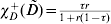${\textstyle{{\tau r} \over {1 \plus r\lpar 1 \minus \tau \rpar }}}$ , $\chi _{D}^{ \plus } \lpar \tilde{D}\rpar \equals {\textstyle{{\tau r} \over {1 \plus r\lpar 1 \minus \tau \rpar }}}$ for some $\tilde{D} \gt 0$ , and χ_D ⁺(D)→∞ as D→∞.

The value $\tilde{D}$ defines the debt where marginal intermediation costs match the tax benefit, and so net costs are zero: $\chi _{D} \lpar \tilde{D}\rpar \equals \lpar 1 \minus {\textstyle{{r\tau } \over {1 \plus r}}}\rpar \chi _{D}^{ \plus } \lpar \tilde{D}\rpar \minus {\textstyle{{r\tau } \over {1 \plus r}}} \equals 0$ .

Because $\bar{\chi }_{D}^{ \plus } \lpar D\rpar \lt \chi _{D}^{ \plus } \lpar D\rpar$ , average intermediation costs are strictly less than the tax benefit for all $D\leqslant \tilde{D}$ ; by continuity, $\bar{\chi }_{D}^{ \plus } \lpar D\rpar \lt 0$ holds for a range D-values greater than $\tilde{D}$ . In this range, the average interest rate on municipal debt, $\lpar 1 \plus r \minus r\tau \rpar \lpar 1 \plus \bar{\chi }_{D}^{ \plus } \lpar D\rpar \rpar \minus 1$ , is less than r. Empirical data showing municipal yields below Treasury yields are therefore consistent with net intermediation costs that are positive on the margin.

To account for pension funding, consider the retirement fund as separate entity from other government operations. Assume the government pays cash wages w_t ¹L_t ¹+w_t ²L_t ² directly to employees and contributes P_t to a pension fund. Given an initial fund balance F_t ⁰, end-of-period fund assets are F_t=F_t*+P_t−B_t, and F_t ₊₁⁰=(1+r)F_t.

In the regular budget, property taxes on $\bar{N}$ homes pay for cash wages and for pension contributions. Given initial debt D_t ⁰, end-of-period debt is $D_{t} \equals D_{t}^{\setnum{0}} \plus w_{t}^{\setnum{1}} L_{t}^{\setnum{1}} \plus w_{t}^{\setnum{2}} L_{t}^{\setnum{2}} \plus P_{t} \minus \bar{N} \cdot T_{t}$ , and D_t ₊₁⁰=(1+r−rτ)(1+χ_D ⁺(D))D_t. Combining regular and pension budgets,

(12)

$D_{t} \minus F_{t} \equals D_{t}^{\setnum{0}} \minus F_{t}^{\setnum{0}} \plus B_{t} \plus w_{t}^{\setnum{1}} L_{t}^{\setnum{1}} \plus w_{t}^{\setnum{2}} L_{t}^{\setnum{2}} \minus \bar{N} \cdot T_{t}.$

Assuming that investors impose the transversality condition lim_n_→∞(D_t _+n−F_t _+n)/(1+r)ⁿ=0, one obtains an intertemporal budget constraint (IBC)

(13)

$\hskip-2pt \mathop{\sum}\limits_{n\geqslant \setnum{0}} {\left( {{1 \over {1 \plus r}}} \right)^{n} } \left( {\bar{N} \cdot T_{t \plus n} } \right) \equals\hskip-3pt \mathop{\sum}\limits_{n\geqslant \setnum{0}} {\left( {{1 \over {1 \plus r}}} \right)^{n} } W_{t \plus n} \plus D_{t}^{\setnum{0}} \plus B_{t} \minus F_{t}^{\setnum{0}} \plus \hskip-3pt \mathop{\sum}\limits_{n\geqslant \setnum{0}} {\left( {{1 \over {1 \plus r}}} \right)^{n} } \bar{\chi }_{D} \lpar D_{t \plus n} \rpar D_{t \plus n} \comma$

where $W_{t} \equals w_{t}^{\setnum{1}} L_{t}^{\setnum{1}} \plus w_{t}^{\setnum{2}} L_{t}^{\setnum{2}} \plus {\textstyle{1 \over {1 \plus r}}}B_{t \plus n \plus \setnum{1}}$ captures compensation for period-t labor.Footnote ¹⁵ Because property taxes are capitalized, home prices are

(14)

$\eqalign{ H_{t} \equals \tab {{1 \over {\bar{N}}}}\mathop{\sum}\limits_{n\geqslant \setnum{0}} {\left( {{1 \over {1 \plus r}}} \right)^{n} } \left( {v\lpar g_{t \plus n} \rpar \minus W_{t \plus n} \minus \chi _{H} } \right) \minus {\textstyle{1 \over {\bar{N}}}}\left( {D_{t}^{\setnum{0}} \plus B_{t} \minus F_{t}^{\setnum{0}} } \right) \cr \tab \plus {{1 \over {\bar{N}}}}\mathop{\sum}\limits_{n\geqslant \setnum{0}} {\left( {{1 \over {1 \plus r}}} \right)^{n} } \left( {{{r\tau } \over {1 \plus r}} \minus \left( {1 \minus {{r\tau } \over {1 \plus r}}} \right)\bar{\chi }_{D}^{ \plus } \lpar D_{t \plus n} \rpar } \right)D_{t \plus n} \cr}$

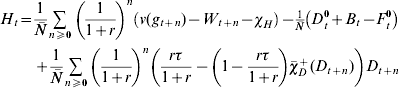
using (2) and (13), where ${\textstyle{{r\tau } \over {1 \plus r}}} \minus \lpar 1 \minus {\textstyle{{r\tau } \over {1 \plus r}}}\rpar \bar{\chi }_{D}^{ \plus } \lpar D_{t \plus n} \rpar \equals \minus \bar{\chi }_{D} \lpar D_{t \plus n} \rpar$ . Equation (14) shows how house prices depend on government policy: The first term is the present value of government services minus labor costs; the second term shows that initial debt D_t ⁰ and unfunded pension promises B_t−F_t ⁰ reduce H_t; the third term shows that the tax benefits of municipal debt and the average intermediation costs are also capitalized.

Note that the tax benefits of municipal debt net of intermediation costs would be maximized if $D_{t \plus n} \equals \tilde{D}\forall n$ . At $\tilde{D}$ , ${\textstyle{{r\tau } \over {1 \plus r}}} \minus \lpar 1 \minus {\textstyle{{r\tau } \over {1 \plus r}}}\rpar \bar{\chi }_{D}^{ \plus } \lpar \tilde{D}\rpar \gt 0$ , and so the tax-deductibility of municipal interest adds value to the house. (By comparison, debt $D_{t \plus n} \lt \tilde{D}$ would fail to exploit the tax benefits; debt $D_{t \plus n} \gt \tilde{D}$ would have marginal costs greater than tax benefits.).

3.4. Voting over local government policy

Two voting scenarios are of interest in this setting – repeated voting with discretion, and voting constrained by fiscal rules.

First consider discretionary voting, which means that voters set current policy variables and take future policy as given. One finds:

Proposition 2 Under Assumptions 1–4, with discretionary voting:

(a) Voter references over pension funding F_t and over public debt D_t are single peaked.
(b) For all voters, F_t=0 maximizes utility, regardless of initial conditions.
(c) For each voter (age i), the preferred debt Dⁱ equates the marginal costs of public debt net of tax benefits with the marginal costs of the voter's own debt:
(15)
$\chi _{D} \lpar D^{i} \rpar \equals \left( 1 \minus {{r\tau } \over {1 \plus r}}\right) \chi _{D}^{ \plus } \lpar D^{i} \rpar \minus {{r\tau } \over {1 \plus r}} \equals \chi _{d}^{i} \lpar d_{d}^{i\ast } \rpar \comma$
So Dⁱ≡(χ_D)⁻ ¹ (χ_dⁱ(d_dⁱ*)).

Proposition 2 confirms that zero pension funding is optimal for all voters. Proposition 2 also shows that taxpayers with personal debts have an incentives to vote for more public debt until the marginal costs of public debt matches their own borrowing costs.

The equilibrium debt is D_t=D ¹ or D_t=D ², depending on the median voter's age. Note that both exceed $\tilde{D}$ . If the intermediation costs χ_D ⁺ are small at first, equilibrium debt may be extremely high. Moreover, voters and investors must anticipate that $D_{t \plus n} \equals D^{i} \gt \tilde{D}$ for all n, which reduces house prices relative to $\tilde{D}$ . Irrespective of current debt, if voters were able to control future debt, they would like to set $D_{t \plus n} \equals \tilde{D}$ for all n⩾1, i.e., they would value a mechanism that limit future debt.

Hence, consider fiscal rules. To avoid tedious case distinctions, assume that the middle aged are the majority (N ²>N ¹), so the discretionary outcome is D_t=D ²∀t, and that χ_d ²(d_d ^2*)⩽χ_d ¹(d_d ^1*), so D ²⩽D ¹. Then two questions arise.

First, if voters could enact a permanent debt limit $\ \ihats{D}$ for themselves and for all future periods (so $D_{t \plus n} \leqslant \ \ihats {D} \ \forall n$ ), would they do so? Because any limit $\ \ihats{D}\ \leqslant \, D^{\setnum{2}}$ would hold with equality, the optimal debt limit ( $\ \ihats {D}\hskip1.5pt ^{\setnum{2}\ast}$ ) is found by maximizing voter utility with respect to $\ \ihats{D}$ . The first-order condition can be written as

(16)

$\left( 1 \minus {{r\tau } \over {1 \plus r}}\right) \chi _{D}^{ \plus } \lpar D^{\setnum{2}\ast } \rpar \minus {{r\tau } \over {1 \plus r}} \equals \chi _{D} \lpar D^{\setnum{2}\ast } \rpar \equals {{r\lpar 1 \plus r\rpar } \over {1 \plus r\lpar 1 \plus r\rpar }}\chi _{d}^{\setnum{2}} \lpar d_{d}^{\setnum{2}\ast } \rpar.$

Since $0 \lt {\textstyle{{r\lpar 1 \plus r\rpar } \over {1 \plus r\lpar 1 \plus r\rpar }}} \lt 1$ , $\ \ihats{D}\hskip2pt^{\setnum{2}\ast }$ is strictly less than D ², though greater than $\tilde{D}$ . The outcome $D_{t} \equals \ \ihats{D}\hskip2pt^{\setnum{2}\ast } \forall t$ yields higher utility for middle-aged voters than the discretionary equilibrium.Footnote ¹⁶

Second, how can debt limits be enforced? Game theory provides an answer:

Proposition 3 There is a range of debt limits $\lsqb \ \ihats{D}\, _{\min } \comma \ \ihats{D}\, _{\max } \rsqb$ , which includes $\ \ihats{D}\hskip2pt^{\setnum{2}\ast }$ so that for any $\ \ihats{D}\ \in \lsqb \ \ihats{D}\, _{\min } \comma \ \ihats{D}\, _{\max } \rsqb$ , $D_{t \plus n} \equals \ \ihats{D}\ \forall n$ is a sequential equilibrium in a repeated voting game with the following trigger strategies: $D_{t} \equals \ \ihats{D}$ if $D_{i} \leqslant \ \ihats{D}\ \forall i \lt t$ , and D_t=D ² otherwise.

Assuming that an initial middle-aged generation can choose $\ \ihats{D}\, \in \lsqb \ \ihats{D}\, _{\min } \comma \ \ihats{D}\, _{\max } \rsqb$ , it chooses $\ \ihats{D} \equals \ \ihats{D}\hskip2pt^{\setnum{2}\ast }$ , and so the equilibrium debt is $D_{t} \equals \ \ihats{D}\hskip2pt^{\setnum{2}\ast } \, \forall t$ . One can show that young voters also support a range of debt limits, and that this range includes $\ \ihats{D}\hskip2pt ^{\setnum{2}\ast }$ provided χ_d ¹(d_d ¹*) and χ_d ²(d_d ^2*) are not too far apart. Then $\ \ihats{D}\hskip2pt^{\setnum{2}\ast }$ is a Pareto improvement over both D ¹ and D ².

Constitutional and procedural rules that regulate voting on debt are empirically relevant. Most U.S. states and local government operate in a balanced-budget setting that allows debt issues only for capital projects. Note that if ${\textstyle{{r\lpar 1 \plus r\rpar } \over {1 \plus r\lpar 1 \plus r\rpar }}}$ is small, the debt $\ \ihats{D}\hskip2pt^{\setnum{2}\ast }$ has net marginal costs close to zero. Hence, the prediction of the model is that fiscal rules should allow public debt up to a level where the marginal costs roughly match the tax benefits, but not much more. One may suspect that capital debt can be evaluated easily by lenders and ratings agencies and has low intermediation costs, whereas unsecured or ‘floating’ debt would require extensive due diligence – to avoid adverse selection – and monitoring. Hence, the model is broadly consistent with U.S. fiscal rules.Footnote ¹⁷

Returning to pension funding, the main conclusion is that rational voters have reason to support balanced-budget-type constraints on public debt. Importantly, there is no parallel argument that would justify constraints on pension funding. Zero pension funding is the unique preferred outcome for all voters in all periods. Hence, it is proper for balanced-budget rules to be silent about pension funding.

A further implication is that if an outside regulator or national government were to restrict debt relative to the discretionary outcome, voters should approve. But if a regulator were to impose minimum funding requirements on public pensions (say, F_t⩾F _min>0), such restrictions would reduce utility for everyone.Footnote ¹⁸

The possibility that pension returns differ from the market interest rate is worth discussing. If pension returns were less, e.g., because public pension funds are costly to administer, voters’ aversion to funding would be strengthened. Conversely, if pension funds earned reliably above-market returns, the effective cost of funding would be reduced. Voters who have sufficiently great expectations about active fund management would favor funding. This may provide a behavioral explanation as to why many public retirement plans are funded.

In summary, the main result is that zero pension funding is optimal for rational taxpayers who face intermediation costs on their own debt. Such taxpayers are also tempted to incur high public debt, but they prefer to support fiscal rules that limit debt. The model implies that such rules should not apply to ‘borrowing’ via unfunded pension promises – thus invalidating popular analogies between debt and underfunded pensions.

4. Legal ambiguity and default risk

Legal ambiguity and pension defaults deserve attention here because they provide rational motives for taxpayers to fund pensions even when funding is costly.

The key issues are (1) uninsurable risk and (2) the role of pension assets as collateral. Employees covered by a DB plan typically rely on a single pension for a large share of retirement consumption. The risk of non-payment is a concentrated risk that is difficult to insure. To attract employees, the employer must compensate for uninsurable risk by offering a wage premium. If pension assets can serve as collateral, funding may reduce the wage premium, perhaps enough to outweigh the intermediation costs argument.

By legal ambiguity I mean the possibility that a plan sponsor can successfully dispute the scope or existence of pension obligations. If a plan sponsor finds a legal flaw or otherwise challenges a pension payment, an insurer could raise the same objections. Hence, employees cannot insure against legal ambiguity. Employees must always worry how the courts might rule, and this uncertainty is uninsurable.

For example, consider a plan that promises a fixed percentage of final salary, which is then indexed to inflation, as is common in DB plans. Final salary is an ambiguous term when the structure of compensation is evolving. A stingy definition – excluding all bonus-type payments – would allow the employer to cut pensions by reducing base salaries and instead paying repeated bonuses. With inflation, freezing nominal salaries would work similarly. A generous definition would invite attempts to manipulate the timing of payments to show an abnormally high final salary – a practice known as ‘pension spiking.’ Indexing clauses may also cause trouble, e.g., if simple formulas become so ‘unreasonable’ over time that a court may not enforce them.

To model legal ambiguity – or more broadly, enforcement problems that create uninsured risk – assume that there are two possible outcomes for the pension plans, indicated by states of nature (s_t ₊₁⁻,s_t ₊₁⁺). In a stochastic setting, they could be interpreted as two outcomes that divide each otherwise identical state of nature. With probability $\bar{\pi }$ , the promised benefits X_t ₊₁ are disputed and the plan sponsor successfully refuses additional contributions. Then beneficiaries share the available funds, and so actual payments are X(s_t ₊₁⁻)=min{X_t ₊₁,F_t ₊₁⁰/L_t ²}. With probability $1 \minus \bar{\pi }$ , promised benefits are honored, so X(s_t ₊₁⁺)=X_t ₊₁. As a behavioral extension, let employees’ perception of enforcement problems be distinct from the employer's view and be denoted by $\bar{\pi }^{e}$ .

For simplicity, assume that $\bar{\pi }$ and $\bar{\pi }^{e}$ are exogenous; that the local government is controlled by middle-aged voters; that voters’ marginal utility is approximately the same in states (s_t ₊₁⁻,s_t ₊₁⁺); and that public employees have power utility with relative risk aversion γ. The government's objective is then (written loosely to avoid elaborate notation) to maximize V_t ² in expected value subject to the government budget constraint and subject to the employment constraint that

(17)

$\lpar 1 \minus \pi \rpar \bar{U}\lpar x_{t}^{\setnum{2}} \comma X_{t \plus \setnum{1}} \rpar \plus \pi \bar{U}\lpar x_{t}^{\setnum{2}} \comma \min \hskip-2pt \lcub X_{t \plus \setnum{1}} \comma F_{t \plus \setnum{1}}^{\setnum{0}} \sol L_{t}^{\setnum{2}} \rcub \rpar \geqslant \bar{U}^{DC}.$

The intuition is that whenever F_t ₊₁⁰/L_t ²<X_t ₊₁, state s_t ₊₁⁻ triggers a discrete loss of retiree consumption as compared to c_t ₊₁³(s ⁺), and hence an upward ‘jump’ in marginal utility. To satisfy (17) with this friction, x_t ² must be reduced by an amount that includes a risk premium. That is, the government must pay wages and benefits with higher expected value than if they could commit to paying benefits with certainty. Let $\rmDelta u' \equals {\textstyle{{u'\lpar c_{t \plus \setnum{1}}^{\setnum{3}} \lpar s^{ \minus } \rpar \rpar \minus u'\lpar c_{t \plus \setnum{1}}^{\setnum{3}} \lpar s^{ \plus } \rpar \rpar } \over {u'\lpar c_{t \plus \setnum{1}}^{\setnum{3}} \lpar s^{ \plus } \rpar \rpar }}}$ be the percentage gap between employees’ marginal utilities between states (s_t ₊₁⁻,s_t ₊₁⁺). With power utility, Δu′ can be expressed in terms of the funding ratio f=F_t ₊₁⁰/(X_t ₊₁L_t ²)⩾0, and the pension dependence ξ=(1−τ³)X_t ₊₁/c_t ₊₁³(s ⁺)⩾0, which is the ratio pension income to total retirement consumption:

$\rmDelta u\prime \lpar f\comma \xi \rpar \equals \lsqb 1 \minus \lpar 1 \minus f\rpar \xi \rsqb ^{ \minus \gamma } \minus 1\geqslant 0.$

Note that Δu′ is decreasing in f, so funding reduces risk, and that both Δu′ and the derivative ∂(Δu′)/∂f are increasing in ξ for all f<1. The latter suggests that funding matters most for retirees who rely heavily on their DB pensions. One finds:

Proposition 4 In a setting with intermediation costs and enforcement problems, the optimal funding ratio f depends on how χ_d ²(d_t ^2*) compares with ${\textstyle{{1 \minus \bar{\pi }} \over {1 \minus \bar{\pi }^{e} }}}\lsqb 1 \plus \bar{\pi }^{e} \cdot \rmDelta u'\lpar f\comma \xi \rpar \rsqb$ :

If ${\textstyle{{1 \minus \bar{\pi }} \over {1 \minus \bar{\pi }^{e} }}}\lsqb 1 \plus \bar{\pi }^{e} \cdot \rmDelta u\prime \lpar 0\comma \xi \rpar \rsqb \leqslant 1 \plus \chi _{d}^{\setnum{2}} \lpar d_{t}^{\setnum{2}\ast } \rpar$ , then f=0. If ${\textstyle{{1 \minus \bar{\pi }} \over {1 \minus \bar{\pi }^{e} }}}\geqslant 1 \plus \chi _{d}^{\setnum{2}} \lpar d_{t}^{\setnum{2}\ast } \rpar$ , then f=1. Otherwise, 0<f<1 is uniquely defined by

(18)

$\lsqb 1 \plus \bar{\pi }^{e} \cdot \rmDelta u'\lpar f\comma \xi \rpar \rsqb {{1 \minus \bar{\pi }} \over {1 \minus \bar{\pi }^{e} }} \equals 1 \plus \chi _{d}^{\setnum{2}} \lpar d_{t}^{\setnum{2}\ast } \rpar.$

The term $1 \plus \bar{\pi }^{e} \rmDelta u\prime \lpar f\comma \xi \rpar$ exceeds one if $\bar{\pi }^{e}$ >0 and if the risk is uninsured (so Δu′(f,ξ)>0). The ratio ${\textstyle{{1 \minus \bar{\pi }} \over {1 \minus \bar{\pi }^{e} }}}$ equals one unless employees and the employer have different perceptions. Two corollaries follow:

(1) Under symmetric expectations, the optimal funding ratio is bounded away from one but not from zero: For $\bar{\pi } \equals \bar{\pi }^{e}$ , equation (18) reduces to $\bar{\pi } \cdot \rmDelta u'\lpar f\comma \xi \rpar \equals \chi _{d}^{\setnum{2}} \lpar d_{t}^{\setnum{2}\ast } \rpar \gt 0$ . Full funding cannot be optimal because Δu′→0 as f→1. The corner solution f=0 applies whenever
$\rmDelta u'\lpar 0\comma \xi \rpar \equals \lpar 1 \minus \xi \rpar ^{ \minus \gamma } \minus 1\leqslant \chi _{d}^{\setnum{2}} \lpar d_{t}^{\setnum{2}\ast } \rpar \sol \bar{\pi }$
and this holds for a range of parameters with low $\bar{\pi }$ , low ξ, and/or high χ_d ²(d_t ^2*) values.
(2) Full funding is not optimal unless employees are more ‘pessimistic’ than the employer: The gap in expectations must be at least $\bar{\pi }^{e} \minus \bar{\pi }\geqslant \lpar 1 \minus \bar{\pi }^{e} \rpar \chi _{d}^{\setnum{2}} \lpar d_{t}^{\setnum{2}\ast } \rpar \gt 0$ .

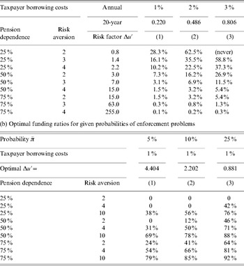
Table 2 illustrates the relationship between optimal funding, pension dependency, and the probability of enforcement problems (legal disputes or default) quantitatively. Panel (a) shows cutoff probabilities for zero funding. Panel (b) shows optimal funding ratios. Generally, high pension dependence, high-risk aversion, and a high degree of legal ambiguity favor funding, whereas intermediation costs discourage funding. The cutoff probabilities in Panel (a) are over 10% for all scenarios with 25% pension dependence and for many of the 50%-dependence scenarios. Thus, zero funding remains optimal unless legal ambiguities are substantial and unless pension dependence is high.Footnote ¹⁹

Table 2.

Pension funding as collateral

(a) Maximum probability of enforcement problems so ZERO funding is optimal

Source: Own calculations, see Section 4. Probability of enforcement problems refers to the probability of legal challenges in case of ambiguity and to the default probability in case of uninsurable defaults.

To focus on scenarios that justify positive funding, all columns in Panel (b) assume low intermediation costs and some rows assume very high risk aversion (up to 10). Some entries are nonetheless under 50%. Funding ratios greater than 80%, which are observed empirically, are optimal with relatively high pension dependence (⩾50%) and high risk-aversion (γ=10). Note that scenarios with high pension dependence are empirically relevant because many state and local government employees are not participating in social security.

In conclusion, legal ambiguity can explain why there is pension funding.

The argument relies, however, on several subtle points that should be noted. First, the argument is about uninsurable risk. If insurance were available, the no-funding result from Section 3 would still apply. Only uninsurable risk produces a wage premium in the sense that the employee values the compensation package less than the employers. Second, outright default is observable and therefore should be insurable. Hence, I focus on legal ambiguity as the most plausible source of uninsurable risk.Footnote ²⁰ Third, the argument applies only if pension assets can provide a floor on benefits when legal ambiguities arise. Pension assets are only credible as collateral if they are irrevocably reserved for benefit payments and cannot be reclaimed by the plan sponsor. Strong regal restrictions against ‘raids’ by plan sponsors are indeed common, even when a plan seems vastly overfunded. Such restrictions are difficult to rationalize except by legal ambiguity.Footnote ²¹ Moreover, many retirement funds have a governance structure designed to protect beneficiaries, e.g., through board representation. These design features suggest that legal ambiguities are a concern.

5. Accounting implications of intermediation costs

This section comments briefly on accounting implications. How should governments account for unfunded pension obligations when taxpayers face intermediation costs?

To be specific, consider a DB plan as modeled in Section 3 that promises X_t ₊₁=(1+r)x_t ² to government employees who receive wages w_t ²=ew−x_t ². Total benefits are B_t ₊₁=X_t ₊₁L_t ².

Investors and taxpayers disagree on how to value these benefits. Outside investors who use market rates for discounting compute the accrued actuarial liability as AAL_t^m=B_t ₊₁/(1+r)=x_t ²L_t ². Taxpayers discount the future by (1+r)(1+χ_d(d)), so

${\rm AAL}_{t} \equals {1 \over {1 \plus \chi _{d} \lpar d\rpar }}x_{t}^{\setnum{2}} L_{t}^{\setnum{2}} \equals {1 \over {1 \plus \chi _{d} \lpar d\rpar }}{\rm AAL}_{t}^{m} \lt {\rm AAL}_{t}^{m}.$

To explain the practical implications, it helps to include risk premiums explicitly. The analysis of Section 3 applies analogously to a setting with uncertain asset returns and state-contingent retirement benefits, provided r is replaced by an stochastic pricing kernel, m_t ₊₁. Then outside investors’ value (possibly state-contingent) benefits B_t ₊₁ at AAL_t^m=E_t[m_t ₊₁B_t ₊₁]. Taxpayers who face intermediation costs have a marginal rate of substitution ${\textstyle{{\beta u'\lpar \hat{c}_{t \plus \setnum{1}}^{i} \rpar } \over {u'\lpar \hat{c}_{t}^{i} \rpar }}} \equals {\textstyle{{m_{t \plus \setnum{1}} } \over {1 \plus \chi _{d} \lpar d\rpar }}}$ that discounts the future more than m_t ₊₁. Hence, they value the same pension benefit at

(19)

${\rm AAL}_{t} \equals E_{t} \left[ {{{m_{t \plus \setnum{1}} } \over {1 \plus \chi _{d} \lpar d\rpar }}B_{t \plus \setnum{1}} } \right] \equals {1 \over {1 \plus \chi _{d} \lpar d\rpar }}{\rm AAL}_{t}^{m}.$

The disagreement about discounting is the same with and without uncertainty. Either way, the relevant discount rate for taxpayers includes an allowance for intermediation costs, i.e., it should be derived from taxpayers’ borrowing costs, which is higher than the risk-adjusted interest rates available to investors.

This argument for a higher discount rate should not be confused with accounting arguments that link discount rates to assets returns (e.g. GASB). The discount rate in (19) depends on the risk characteristics of pension liabilities; it is unrelated to the pension fund's expected investment return or funding status.

In applications, adjusting for intermediation costs means adding a spread to investment-based discount rates. For example, consider a plan with ‘safe’ benefits that are often discounted at duration-matched Treasury rates (Novy-Marx and Rauh, Reference Novy-Marx and Rauh2009). Over the last 20 years, 10-year Treasuries yields have averaged 2.8% in real terms (5.6% nominal, 2.8% inflation). If the median voter faces an intermediation cost of 1–3%, one obtains real discount rates of about 4–6%.Footnote ²² For pension benefits subject to default risk, one would have to add a risk premium, e.g., the spread between taxable municipal bond and Treasuries (say 1%). This suggests real discount rates in the 5–7% range, or nominal 8–10%. These values are comparable to the 7–8% discount rates commonly used by accountants – and perhaps higher for highly indebted taxpayers. Thus, though accountants’ reasoning is questionable, their discount rates are not unreasonable.

One complication is that because funding is suboptimal, measures of ‘underfunding’ are difficult to interpret. A fund with assets F_t has an expected funding gap at the start of the next period of

(20)

$\eqalign{{\rm UAAL}_{t} \equals \tab E_{t} \left[ {{{m_{t \plus \setnum{1}} } \over {1 \plus \chi _{d} \lpar d\rpar }}\left( {B_{t \plus \setnum{1}} \minus F_{t \plus \setnum{1}}^{\ast } } \right)} \right] \equals {\rm AAL}_{t} \minus {1 \over {1 \plus \chi _{d} \lpar d\rpar }}F_{t} \cr \equals \tab \lpar {\rm AAL}_{t} \minus F_{t} \rpar \plus {{{\chi _{d} \lpar d\rpar } \over {1 \plus \chi _{d} \lpar d\rpar }}}F_{t} \comma}$

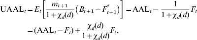
which is positive even if one starts with F_t=AAL_t. The last term in (20) captures taxpayers’ intermediation costs. Hence, a forward-looking measure of underfunding must include not only the current funding gap AAL_t−F_t but also a charge for the funding costs that are suboptimal for taxpayers. Overall, intermediation costs have accounting implications that differ significantly from the standard approaches in finance and accounting.

6. Concluding comments

The paper examines optimal public pension arrangements in a setting where many taxpayers are borrowers, and borrowers face intermediation costs.

In a benchmark model constructed so that all interested voters are debtors, zero funding is an optimal policy for public pensions. It is utility maximizing for everyone, and hence the unique Pareto optimum. The basic argument is that intermediation costs create a wedge between the costs of borrowing and the returns on financial assets. Indebted taxpayers are then better off if they, instead of paying taxes to fund public pensions, leave pensions unfunded, defer the taxes until pension payouts are due, and use the tax-deferral to reduce their own debt.

In practical terms, the question is: Why should taxpayers vote to accumulate assets in a public retirement plans that buys Treasury notes yielding, say, 2% when they are paying 14% interest on their credit cards and 7% on car loans? Although part of the spreads between consumer loans and Treasury rates undoubtedly reflects default premiums, another part reflects intermediation costs. Even Prime borrowers pay spreads of about 3% over T-bills. More than 75% of U.S. families hold debt. They could avoid the intermediation costs by underfunding public pensions and thereby deferring taxes.

The model has two other noteworthy features. First, despite households’ incentives to borrow and to underfund public pensions, the model is consistent with fiscal rules that limit public debt. The intuition is that because of indebted voters’ strong incentives to incur public debt, an unconstrained equilibrium would result in an excessive debt (as formalized in the model). Hence, voters have reason to support a debt limit even if it restricts their own ability to issue public debt. Second, the model implies that unfunded pension obligations should be discounted at an interest rate that includes intermediation costs. This is relevant to the current debate about GASB rules. It implies that discounting future pension obligation at interest rates significantly greater than Treasury rates is consistent with economic theory.

Although the main model is deterministic, the argument generalizes straightforwardly to a stochastic setting. For any asset class, if returns to pension assets and returns to taxpayer debt are adjusted for risk, there is a gap that equals the costs of intermediation. Fees for fund management would widen the gap – unless voters are gullible enough to believe that pension managers can earn abnormal returns that justify all the costs.

The basic model abstracts from complications that may justify pension funding. In an extension, I focus on legal ambiguity – the risk that unfunded pension promises may not be enforceable – as an important complication. If pension assets provide credible collateral, they avoid a risk-related wage premium, and so funding can be optimal for taxpayers subject to intermediation costs. The collateral function can explain why retirement plans are legally structured so that assets are irrevocably committed to pay plan benefits. The extended model with legal ambiguity is broadly consistent with the fact that most public retirement plans are funded, but assets usually fall short of full funding.

Appendix: Proofs

Proposition 1 Let μ(z)⩾0 denote the Kuhn–Tucker multiplier for any constraint z⩾0. The optimality conditions for (x_t ₊₁²,a_t ₊₁²,d_t ₊₁²) can be written as

$\eqalign{{{u\prime\lpar \hskip2pt\hat{c}_{t \plus \setnum{1}}^{\setnum{2}} \rpar } \over {\beta \lpar 1 \plus r\rpar u'\lpar c_{t \plus \setnum{2}}^{\setnum{3}} \rpar }} \equals \tab{{1 \minus \tau ^{\setnum{3}} } \over {1 \minus \tau ^{\setnum{2}} }} \minus {{\mu \lpar x_{t \plus \setnum{1}}^{\setnum{2}} \rpar } \over {\beta \lpar 1 \plus r\rpar u\prime \lpar c_{t \plus \setnum{2}}^{\setnum{3}} \rpar }} \equals {{1 \plus r\lpar 1 \minus \tau ^{\setnum{3}} \rpar } \over {1 \plus r}} \plus {{\mu \lpar a_{t \plus \setnum{1}}^{\setnum{2}} \rpar } \over {\beta \lpar 1 \plus r\rpar u'\lpar c_{t \plus \setnum{2}}^{\setnum{3}} \rpar }} \cr\equals \tab 1 \plus \chi _{d} \lpar d_{t \plus \setnum{1}}^{\setnum{2}} \rpar \minus {{\mu \lpar d_{t \plus \setnum{1}}^{\setnum{2}} \rpar } \over {\beta \lpar 1 \plus r\rpar u'\lpar c_{t \plus \setnum{2}}^{\setnum{3}} \rpar }}}$

Since ${\textstyle{{1 \minus \tau ^{\setnum{3}} } \over {1 \minus \tau ^{\setnum{2}} }}} \gt 1\ges {\textstyle{{1 \plus r\lpar 1 \minus \tau ^{\setnum{3}} \rpar } \over {1 \plus r}}}$ , μ(a_t ₊₁²)>0, so a_t ₊₁^2*=0. Then c_t ₊₂³>H_t ₊₂+TR_t ₊₂ implies x_t ₊₁²>0, hence μ(x_t ₊₁²)=0 and ${\textstyle{{{\rm MRS}^{\setnum{23}} } \over {1 \plus r}}} \equals {\textstyle{{u'\lpar \hskip1.5pt \hat{c}_{t \plus \setnum{1}}^{\setnum{\hskip1pt 2}} \rpar } \over {\beta \lpar 1 \plus r\rpar u'\lpar c_{t \plus \setnum{2}}^{\setnum{3}} \rpar }}} \equals {\textstyle{{1 \minus \tau ^{\setnum{3}} } \over {1 \minus \tau ^{\setnum{2}} }}} \equals 1 \plus R^{\setnum{23}} \equals 1 \plus \chi _{d} \lpar d_{t \plus \setnum{1}}^{\setnum{2}} \rpar$ , which proves d_t ₊₁^2*=(χ_d ²)⁻ ¹(R ²³). In young age, c_t ¹>w and h_t ¹=1 implies $d_{t}^{\setnum{1}} \gt H_{t} \gt \tilde{d}$ , so μ(d_t ¹)=0 and χ_d(d_t ¹)>0. Using MRS²³=(1+r)(1+R ²³), the optimality conditions for (x_t ¹,a_t ¹,d_t ¹) can be written as

${{{u'\lpar \hskip1pt\hat{c}\hskip1pt_{t}^{\setnum{1}} \rpar } \over {\beta \lpar 1 \plus r\rpar u'\lpar \hskip1pt \hat{c}_{t \plus \setnum{1}}^{\setnum{ \hskip1pt 2}} \rpar }}} \equals {{1 \minus \tau ^{\setnum{2}} } \over {1 \minus \tau ^{\setnum{1}} }} \minus {{\mu \lpar x_{t}^{\setnum{1}} \rpar } \over {\beta \lpar 1 \plus r\rpar u'\lpar \hskip1pt \hat{c}_{t \plus \setnum{1}}^{\setnum{\hskip1pt 2}} \rpar }} \equals {{1 \plus r\lpar 1 \minus \tau ^{\setnum{2}} \rpar } \over {1 \plus r}} \plus {{\mu \lpar a_{t}^{\setnum{1}} \rpar } \over {\beta \lpar 1 \plus r\rpar u'\lpar\hskip1pt \hat{c}_{t \plus \setnum{1}}^{\setnum{\hskip1pt 2}} \rpar }} \equals 1 \plus \chi _{d} \lpar d_{t}^{\setnum{1}} \rpar$

Because 1+χ_d(d_t ¹)>1, whereas ${\textstyle{{1 \minus \tau ^{\setnum{2}} } \over {1 \minus \tau ^{\setnum{1}} }}}\leqslant 1$ and ${\textstyle{{1 \plus r\lpar 1 \minus \tau ^{\setnum{2}} \rpar } \over {1 \plus r}}} \lt 1$ , μ(a _t¹)>0 and μ(x _t¹)>0 follow, so x _t¹=a_t ¹=0.

Proposition 2 Follows from differentiating (1) subject to (12), (14) and $\bar{U}\lpar x_{t}^{\setnum{2}} \comma X_{t \plus \setnum{1}} \rpar \geqslant \bar{U}^{{\rm DC}}$ .

Proposition 3 Consider the middle-aged voter's problem of maximizing (1) subject to (12), (14) and $\bar{U}\lpar x_{t}^{\setnum{2}} \comma X_{t \plus \setnum{1}} \rpar \geqslant \bar{U}^{{\rm \hskip1pt DC}}$ with $D_{t \plus n} \equals \ \ihats{D}\ \forall n\geqslant 1$ and given D_t, and let $U^{\ast}\lpar D_{t} \comma \ \ihats{D}\, \rpar$ denote the maximum utility for given $\lpar D_{t} \comma \ \ihats{D}\, \rpar$ . Straightforward differentiation yields $\ \ihats{D}\hskip2pt^{\setnum{2}\ast } \equals \arg \max _{\ \ihats{D}} U^{\ast } \lpar \ \ihats{D}\, \comma \ \ihats{D}\, \rpar$ with ${\rm d}U^{\ast } \lpar \ \ihats{D}\,\comma \ \ihats{D}\,\rpar \sol {\rm d}\ \ihats{D}$ positive/negative below/above $\ \ihats{D}\hskip2pt^{\setnum{2}\ast }$ . Define $\ \ihats{D}_{\hskip2pt \min } \equiv \min \lcub \ \ihats{D}\,\geqslant 0\colon U^{\ast } \lpar \ \ihats{D}\hskip2pt \comma \ \ihats{D}\hskip2pt \rpar \geqslant U^{\ast } \lpar D^{\setnum{2}} \comma D^{\setnum{2}} \rpar \rcub$ and $\ \ihats{D}_{\ \max } \equiv D^{\setnum{2}}$ , where $\ \ihats{D}_{\ \min } \lt \ \ihats{D}\hskip2pt^{\setnum{2}\ast }$ because $U^{\ast } \lpar \ \ihats{D}\hskip2pt^{\setnum{2}\ast } \comma \ \ihats{D}\hskip2pt^{\setnum{2}\ast }\rpar \gt U^{\ast } \lpar D^{\setnum{2}} \comma D^{\setnum{2}} \rpar$ . If future voters follow the assumed trigger strategy with given $\ \ihats{D}$ , period-t voters can choose either $D_{t} \leqslant \ \ihats{D}$ which yields $\max _{D_{t} \leqslant \ \ihats{D}} U^{\ast } \lpar D_{t} \comma \ \ihats{D}\hskip2pt \rpar \equals U^{\ast } \lpar \ \ihats{D}\hskip2pt \comma \ \ihats{D}\hskip2pt \rpar$ ; or $D_{t} \gt \ \ihats{D}$ , which yields max_{D_t}U*(D_t,D ²)=U*(D ²,D ²). By construction of $\ \ihats{D}_{\hskip2pt \min }$ , the former is preferred if $\ \ihats{D} \hskip2pt \in\lsqb \ \ihats{D}_{ \hskip2pt \min } \comma D^{\setnum{2}} \rpar$ , and so $\ \ihats{D} \hskip2pt \in \lsqb \ \ihats{D}_{ \hskip2pt \min } \comma \hskip3pt \ihats{D}_{\hskip2pt\max } \rsqb$ with $D^{\setnum{2}} \equals \ \ihats{D}_{\hskip2pt \max }$ is sustainable. QED.

Proposition 4 Equation (18) follows from differentiating the expected value of V_t ² with respect to F_t, subject to (12), (14), and (17).

Footnotes

¹ The paper does not address the cost and benefits of DB versus DC plans per se, except with regard to funding. Bohn (Reference Bohn2010) comments on DB versus DC more broadly. See Friedberg (Reference Friedberg2010) for a review for labor market issues.

² For example, according to a November 2009 CNN poll, 67% of U.S. voters agree that ‘the government should balance the budget even when the country is in a recession and is at war.’

³ Such information problems do not imply ‘fiscal illusion’ – the notion that voters underestimate the long-run cost of deficit-financed expenditures. The issue here is risk reduction. An appropriate analogy is the question how much signature authority to give to an accountant – control over current accounts or also the power to borrow.

⁴ Special considerations apply for home mortgages, because the interest is tax-deductible for itemizers and it may reflect federal subsidies to housing lenders. Less than half of all mortgage holders itemize, and many of them hold other debts, too. Hence for most homeowners, the marginal cost of funds exceeds the safe interest rate.

⁵ Home ownership is a convenient device to make voters care about the community's long run future without having to model intergenerational altruism.

⁶ I abstract from uncertainty only to simplify the exposition. An earlier working paper (Bohn, Reference Bohn2010), which includes a stochastic model with arbitrary state-contingent returns, uncertain wages, and defaultable debt, shows that the results here are also valid under uncertainty. In the stochastic version, a pricing kernel replaces the discount factor 1/(1+r) and one must take expectations over states of nature; the economic arguments and the results are completely analogous.

⁷ The assumption of management is needed to ensure that all residents will buy a house.

⁸ Individual IRA accounts deliver similar tax benefits as retirement plans and can be subsumed here under DC plans. It is beyond the scope of this paper to explain why Congress has enacted laws that in effect subsidize pension savings. My focus is on the implications.

⁹ This simple argument ignores restrictions on early withdrawal. This is not a limitation here because in this model, the middle aged will make positive contributions.

¹⁰ Parameters that satisfy Assumption 3 exist. For example, suppose w=1, ew=1.5, the interest rate is 2% annually for a 20-year generational period, and β=1/(1+r). Assume H is five times the annual wages, property taxes are 1% annually, so H=0.25 and T=0.05 per 20-year period. Assume v(g)=0.2, which is consistent with H=0.25 for χ_H=6.8%, and TR=0.5. Assuming taxes and borrowing cost are approximately zero, one finds that home ownership is optimal and $\tilde{c}^{\setnum{1}} \equals \tilde{c}^{\setnum{2}} \equals c^{\setnum{3}} \approx 1.11$ . Assumption 3 is satisfied because w=1 and H+TR=0.75 are less than consumption.

¹¹ For example, consider utility (1) for the middle-aged in period t (which is U_t₋ ₁), insert (7) and (8) and h_t ¹=h_t ²=1∀t. Taking the total differentials of U_t₋ ₁ and of V_t ² with respect to (g_t,T_t,H_t ₊₁) one finds

$\eqalign{ {\rm d}U_{t \minus \setnum{1}} \tab \equals \beta u'\lpar \tilde{c}_{t \plus \setnum{1}} \rpar \lpar v'{\rm d}g_{t \plus \setnum{1}} \minus {\rm d}T_{t \plus \setnum{1}} \rpar \plus \beta ^{\setnum{2}} u'\lpar c_{t \plus \setnum{2}} \rpar {\rm d}H_{t \plus \setnum{1}} \cr \tab \equals \beta u'\lpar \tilde{c}_{t \plus \setnum{1}} \rpar \left\{ {v'{\rm d}g_{t \plus \setnum{1}} \minus {\rm d}T_{t \plus \setnum{1}} \plus {\textstyle{{\beta u'\lpar c_{t \plus \setnum{2}} \rpar } \over {u'\lpar \tilde{c}_{t \plus \setnum{1}} \rpar }}}{\rm d}H_{t \plus \setnum{1}} } \right\} \cr \tab \equals \beta u'\lpar \tilde{c}_{t \plus \setnum{1}} \rpar {\rm d}V_{t}^{\setnum{2}} \cr}$

so changes in V_t ² are proportional to changes in utility.

¹² The model abstracts from many important differences between DB and DC (see Friedberg, Reference Friedberg2010), but this helps focus on the paper's main question, the choice of funding.

¹³ A formal proof that optimal DB pensions pay w_t ¹=w would be straightforward but lengthy, because one would have to define notation for multi-period pension accruals. In practice, legal restrictions may force DB plan sponsors to include the young. While the paper is not set up to examine accrual methods, the optimality of x_t ^1*=0 suggests caution in using accounting methods (such as entry-age-normal) that mechanically allocate projected benefits over an entire career.

¹⁴ The interpretation is that municipal debt buyers are a special group of outside investors that gains a tax advantage from holding municipal debt. Their tax rate τ may differ from local residents’ tax rates.

¹⁵ Rational investors will also impose a natural debt limit, which is that taxes cannot make house prices negative. I assume public services are sufficiently valuable that house prices are positive for all policies considered in this section.

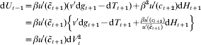
¹⁶ As proof, note that $\ \ihats{D} \equals D^{\setnum{2}}$ is a feasible debt limit but not optimal.

¹⁷ To be precise, the game-theoretic interpretation of fiscal rules is that voters abide by such rules (say, a balanced budget) because they expect a violation to trigger a string of discretionary outcomes that would yield low utility. Proposition 3 formalizes this intuition. Note that a switch to discretion for a finite number of periods would also sustain a range of debt levels less than D ², so Proposition 3 could be generalized.

¹⁸ A current issue is the regulation of retiree health benefits. They are traditionally unfunded – as consistent with optimal policy here – but GASB 43 has created strong accounting incentives to start funding.

¹⁹ Note that enforcement problems are costly for the plan sponsor even when the problems are not severe enough to justify funding. Whenever employees face uninsured risk, wage costs are greater than they would be under certainty.

²⁰ Default may still be relevant empirically because many public employees are in fact uninsured against employer default, though in theory, they should demand insurance. Alternatively, default insurance may fail to exist because attempts to collect (e.g. on credit default swaps) would involve too many legal uncertainties.

²¹ Otherwise, it would be economically efficient to give the plan sponsor (as residual claimant) the right to recover overfunding. But with legal uncertainty, ‘overfunding’ is not well defined because the scope of obligations is likely part of the dispute. Hence, a right to recover funds would undermine the collateral function.

²² Because intermediation costs generally differ across individuals (as exemplified by age differences in the model), there is no single ‘correct’ discount rate for everyone. Hence, I provide a range of rates; the choice of a particular value is a matter of setting accounting conventions.

References

Alesina, Alberto and Perotti, Roberto (1995) The political economy of budget deficits. IMF Staff Papers 42: 1–31.CrossRef Google Scholar

Bader, Lawrence N. and Gold, Jeremy (2007) The case against stock in public pension funds. Financial Analysts Journal, 63(1): 55–62.CrossRef Google Scholar

Bohn, Henning (2010) Should public retirement plans be fully funded? NBER Working Paper No. 16409, September.CrossRef Google Scholar

Brown, Jeffrey and Wilcox, David (2009) Discounting state and local pension liabilities. American Economic Review, 99(2): 538–542.CrossRef Google Scholar

Bulow, Jeremy (1982) What are corporate pension liabilities? Quarterly Journal of Economics 97(3): 435–452.CrossRef Google Scholar

D'Arcy, Stephen P., Dulebohn, James H. and Oh, Pyungsuk (1999) Optimal funding of state employee pension systems. Journal of Risk and Insurance, 66(3): 345–80.CrossRef Google Scholar

Epple, Dennis and Schipper, Katherine (1981) Municipal pension funding: a theory and some evidence. Public Choice, 37(1): 179–87.CrossRef Google Scholar

Friedberg, Leora (2010) Labor Market Aspects of State and Local Retirement Plans: A Review of Evidence and a Blueprint for Future Research. Mimeo: University of Virginia.Google Scholar

Lucas, Deborah and Zeldes, Stephen (2009) How should pension funds invest? American Economic Review, 99(2): 527–532.CrossRef Google Scholar

Munnell, Alicia, Haverstick, Kelly, Sass, Steven and Aubry, Jean-Pierre (2008) The Miracle of Funding by State and Local Pension Plans. Chestnut Hill, MA: Center for Retirement Research, Boston College.Google Scholar

Munnell, Alicia, Haverstick, Kelly, Sass, Steven, Aubry, Jean-Pierre and Quinby, Laura (2010) The Funding of State and Local Pension Plan: 2009–2013. Chestnut Hill, MA: Center for Retirement Research, Boston College.Google Scholar

Novy-Marx, Robert and Rauh, Joshua D. (2009) The Liabilities and Risks of State-Sponsored Pension Plans. Journal of Economic Perspectives 23(4): 191–210.CrossRef Google Scholar

Peng, Jun (2009) State and Local Pension Fund Management. Boca Raton, FL: Taylor & Francis.Google Scholar

Persson, Torsten and Tabellini, Guido (2000) Political Economics. Cambridge, MA: MIT Press.Google Scholar

Table 1. What percentages of U.S. families are borrowers?

Table 2. Pension funding as collateral(a) Maximum probability of enforcement problems so ZERO funding is optimal

Article contents

Should public retirement plans be fully funded?

Abstract

Information

1. Introduction

2. The problem of pension funding

2.1. The ambiguous meaning of full funding

2.2. Balanced-budget rules and deferred compensation

2.3. Pension returns and taxpayers’ cost of funds

3. A model of local government

3.1. Assumptions and a benchmark allocation

3.2. Voting over policy: intuition

3.3. Constraints on local policy

3.4. Voting over local government policy

4. Legal ambiguity and default risk

5. Accounting implications of intermediation costs

6. Concluding comments

Appendix: Proofs

Footnotes

References

Save article to Kindle

Save article to Dropbox

Save article to Google Drive

Reply to: Submit a response

Your details

You have entered the maximum number of contributors

Conflicting interests