1. Introduction
The mechanisms behind auroral breakup, a sudden increase of auroral strength during the magnetospheric substorm (Akasofu Reference Akasofu1968), are not yet entirely understood. While it is known (Schindler Reference Schindler1975) that the three main events in this process are (a) magnetotail reconnection, (b) cross-tail current reduction and (c) auroral breakup, their exact order has not been conclusively determined. There are two main competing models, the near-Earth neutral line (NENL) model and the current disruption (CD) model.
In the NENL model (Baker et al. Reference Baker, Pulkkinen, Angelopoulos, Baumjohann and McPherron1996), a reconnection of the magnetic field lines in the magnetotail creates jets of plasma that flow earthward and tailward. The earthward jet causes a decrease in the cross-tail current, and then enters the high-latitude atmosphere, where it causes the auroral breakup.
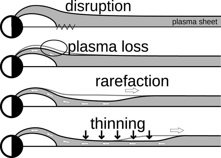
In the CD model (Lui, Meng & Akasofu Reference Lui, Meng and Akasofu1977), a CD instability reduces the cross-tail current, breaking the balance of the near-Earth magnetotail plasma, which enters the high-latitude atmosphere and causes the auroral breakup. The magnetotail plasma loss induces a rarefaction wave in the plasma sheet (figure 1). The tailward propagation of the rarefaction wave causes a reduction of plasma sheet thickness, eventually leading to magnetotail reconnection.
A rarefaction wave causing plasma sheet thinning. Image adapted from Chao et al. (Reference Chao, Kan, Lui and Akasofu1977).

Roughly a decade ago, the THEMIS mission (Angelopoulos Reference Angelopoulos2008) tried to determine which of these two models is the one triggering the auroral substorms. Satellite part of the THEMIS mission is composed of five identical satellite probes distributed and coordinated in the tail of the magnetosphere, which enables us to observe the disturbances in the magnetotail leading to the auroral substorm. To support the satellite observations in space, a number of all-sky cameras were deployed in North America to observe the signature of auroral breakup at the magnetic footprints of the satellites (Mende et al. Reference Mende, Harris, Frey, Angelopoulos, Russell, Donovan, Jackel, Greffen and Peticolas2008). By using the data obtained by the THEMIS mission, Angelopoulos et al. (Reference Angelopoulos, McFadden, Larson, Carlson, Mende, Frey, Phan, Sibeck, Glassmeier and Auster2008) demonstrated an event in which reconnection took place at  $-20 R_{e}$ a few minutes earlier than the signature of current disruption at
 ${\sim }-10 R_{e}$. This observation supports the NENL model, that is, that auroral substorms are initiated by reconnection in the magnetotail. Later, however, Lui (Reference Lui2009) claimed that multisatellite observations during the same interval can be interpreted based on the CD paradigm. Earlier studies by Liou et al. (Reference Liou, Meng, Lui, Newell and Wing2002) of the magnetic field data from GOES 8 and GOES 9 geostationary weather satellites also suggested that the near-Earth reconnection cannot occur before CD, as an unrealistically fast plasma flow speed would be required to satisfy the event timing estimates. Thus, it is still controversial which of these two models better explains the development of the magnetotail disturbances before auroral breakups, and can be regarded as the dominant triggering mechanism of substorms.
In this paper, we consider the CD model. Chao et al. (Reference Chao, Kan, Lui and Akasofu1977) have approximated the initial disturbance that causes the rarefaction wave with an imaginary piston on the near-Earth side of the plasma sheet; earthward movement of the piston generates the rarefaction wave. A simplified model of a piston-bounded one-dimensional (1-D) gas tube was used to approximate the rarefaction wave in the weakly magnetized neutral sheet plasma, and the result was extrapolated to the full plasma sheet. Lui (Reference Lui1991) has stated that to fully assess the ramifications of the rarefaction wave, there is a need to consider a more realistic magnetotail model that includes a non-zero normal magnetic field  $B_z$. We will attempt to move one step closer towards that goal by raising the dimension of the model. However, as a non-zero
 $B_z$ would require a significantly more complicated steady-state configuration than employed in this paper, or even a full three-dimensional simulation, a more comprehensive model will be needed for conclusive results. Nevertheless, we should be able to draw some inferences from simulating the simplified model presented below.
We extend the 1-D model introduced above to a two-dimensional (2-D) vertical cross-section of the plasma sheet, including the north and south magnetic lobes. This allows us to take into account the influence of the strongly magnetized lobe plasma, as well as any dynamics that result from the interaction of plasmas as radically different as sheet and lobe plasma are. We show that, although there is a small drop in pressure, the rarefaction wave, which is supposed to be a signature of the CD model, is not noticeable. Furthermore, the thinning is preceded by a wave train consisting of pulses of increased pressure, generated by the movement of the lobe magnetic field. Since the deformation of the boundary is strongly affected by the physics in the lobe plasma, the propagation velocity of the thinning front shows a strong dependence on lobe conditions.
Preliminary results for this research have been published in an earlier paper (Tretler, Tatsuno & Hosokawa Reference Tretler, Tatsuno and Hosokawa2020), and include a sampling of initially obtained data points with a brief discussion.
This paper is organized as follows. In § 2, we introduce the magnetohydrodynamic (MHD) equations, the physical model of the plasma sheet and the numerical scheme. In §§ 3 and 4, simulation results for the plasma sheet modelled with, respectively, gas equations and MHD equations are presented and discussed. In § 5, we attempt to determine the mechanism behind the thinning by decomposing the system into MHD wave components. In § 6, we compare the results of the 1-D and 2-D models. Finally, concluding remarks are given in § 7.
2. Simulation set-up
2.1. MHD equations
We use the normalized MHD equations in their formulation as a system of conservation laws (Ryu, Jones & Frank Reference Ryu, Jones and Frank1995). System of conservation laws in two dimensions is
 \begin{equation} \frac{\partial \boldsymbol{U}}{\partial t} + \frac{\partial }{\partial x}\boldsymbol{F}(\boldsymbol{U}) + \frac{\partial }{\partial y}\boldsymbol{G}(\boldsymbol{U}) = 0, \end{equation}
where  $\boldsymbol {U}$ is a vector of conserved variables and
 $\boldsymbol {F}(\boldsymbol {U})$ and
 $\boldsymbol {G}(\boldsymbol {U})$ are, respectively, fluxes in
 $x$ and
 $y$ directions. For the ideal MHD system, the conserved variables are
 \begin{equation} \boldsymbol{U} = (\rho , \rho u , \rho v , \rho w , B_x , B_y , B_z , e)^\textrm{T}, \end{equation}
where  $\rho$ is the density,
 $\boldsymbol {u} = ( u, v, w )$ is the velocity vector,
 $\boldsymbol {B} = ( B_x, B_y, B_z )$ is the magnetic field vector and
 $e$ is the total energy. The fluxes in (2.1) are
 \begin{gather} \boldsymbol{F}(\boldsymbol{U}) = \begin{bmatrix} \rho u \\ \rho u u - B_x B_x + p_{\mathrm{total}} \\ \rho v u - B_x B_y \\ \rho w u - B_x B_z \\ 0 \\ B_y u - B_x v \\ B_z u - B_x w \\ u(e + p_{\mathrm{total}}) - B_x(\boldsymbol{u} \boldsymbol{\cdot} \boldsymbol{B})\end{bmatrix}, \end{gather}
 \begin{gather} \boldsymbol{G}(\boldsymbol{U}) = \begin{bmatrix} \rho v \\ \rho u v - B_y B_x \\ \rho v v - B_y B_y + p_{\mathrm{total}} \\ \rho w v - B_y B_z \\ B_x v - B_y u \\ 0 \\ B_z v - B_y w \\ v(e + p_{\mathrm{total}}) - B_y(\boldsymbol{u} \boldsymbol{\cdot} \boldsymbol{B})\end{bmatrix}, \end{gather}
where total pressure  $p_{\mathrm {total}}$ is
 \begin{equation} p_{\mathrm{total}} = p + \tfrac{1}{2} \boldsymbol{B} \boldsymbol{\cdot} \boldsymbol{B} \end{equation}
with plasma kinetic pressure  $p$ defined as
 \begin{equation} p = (\gamma-1) \left( e - \frac{1}{2} \rho \boldsymbol{u} \boldsymbol{\cdot} \boldsymbol{u} - \frac{1}{2} \boldsymbol{B} \boldsymbol{\cdot} \boldsymbol{B} \right), \end{equation}
where  $\gamma$ is the ratio of specific heats, taken to be
 $5/3$.
2.2. Plasma sheet model
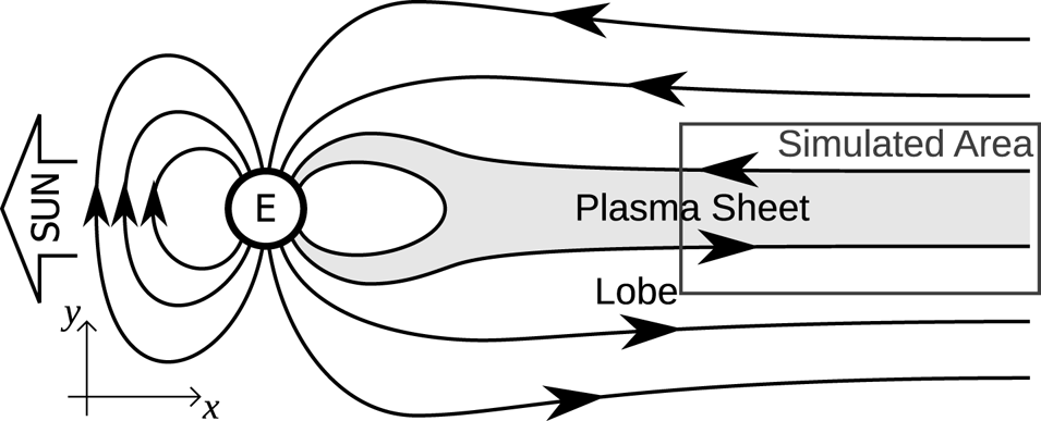
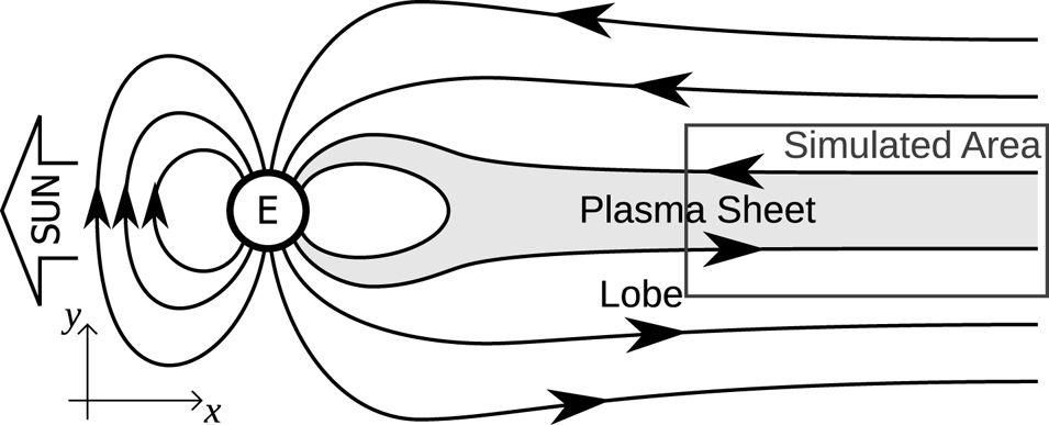
For the simulation, we take the relatively flat area of the plasma sheet, where the magnetic field lines are approximately parallel (figure 2), and look at the  $x$–
 $y$ cross-section, where the
 $x$ axis points from the Earth tailward and the
 $y$ axis points north.
Rough structure of the Earth's magnetosphere, with the simulated area marked.
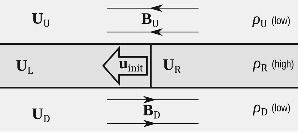
The neutral sheet is composed of a weakly magnetized, high-density plasma,  $\boldsymbol {U}_\mathrm {R}$ (where ‘R’ stands for ‘right’;
 $\boldsymbol {U}_\mathrm {L}$, ‘left’, is the initial disturbance region and will be described later – see figure 3). This plasma is sandwiched between the magnetic lobes, with strongly magnetized, antiparallel, low-density plasmas,
 $\boldsymbol {U}_\mathrm {U}$ (northern lobe, ‘up’) and
 $\boldsymbol {U}_\mathrm {D}$ (southern lobe, ‘down’).
Initial configuration of the simulated area of the plasma sheet.

The inner layer of the plasma sheet,  $\boldsymbol {U}_\mathrm {sheet} = \boldsymbol {U}_\mathrm {R,L}$, was assumed by Chao et al. (Reference Chao, Kan, Lui and Akasofu1977) to have a profile described by
 $\boldsymbol {B}_\mathrm {sheet} = \boldsymbol {B}_\infty \tanh (y)$. However, testing has shown that the results are almost identical if the plasma sheet contains uniform plasma with no magnetic field. Since the latter is more amenable to analysis, we use a uniform plasma sheet as the initial condition for our simulations.
We assume that prior to the disturbance the plasma sheet was in a steady-state configuration, in which case sheet and lobes are separated by tangential discontinuities. The Rankine–Hugoniot jump condition for a tangential discontinuity (Baumjohann & Treumann Reference Baumjohann and Treumann2012) is
 \begin{equation} [p_{\mathrm{total}}] = 0, \end{equation}
where  $[X]$ denotes the jump in
 $X$ when crossing the boundary. With plasma sheet magnetic field
 $\boldsymbol {B}_{\mathrm {sheet}} = \boldsymbol {0}$, and lobe magnetic field pointing in the
 $x$ direction,
 $\boldsymbol {B}_\mathrm {U,D} = \boldsymbol {B}_{\mathrm {lobe}} = ({\pm }B_x, 0, 0)$, this condition becomes
 \begin{equation} p_{\mathrm{sheet}} = p_{\mathrm{lobe}} + \tfrac{1}{2}B_{x,\mathrm{lobe}}^2. \end{equation}
We normalize the system so that  $p_\mathrm {sheet} = 1.0$,
 $\rho _\mathrm {sheet} = 1.0$, and the initial thickness of the plasma sheet is
 $h_\mathrm {sheet} = 1.0$, covering the area
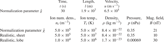
 $-0.5 < y < 0.5$. The relationship between physical and normalized units, as well as realistic values for sheet and lobe obtained from satellite measurements (Baumjohann, Paschmann & Cattell Reference Baumjohann, Paschmann and Cattell1989; Baumjohann & Treumann Reference Baumjohann and Treumann2012), are shown in table 1. With the geometry fixed and physical quantities normalized to sheet conditions, we can fully describe the problem with only a handful of parameters.
Units are normalized with respect to the plasma sheet. In the top half and the first row of the second half are the normalization parameters  $\hat {\chi }$, with the conversion relation for physical quantity
 $\chi$ defined as
 $\chi _\mathrm {real} = \hat {\chi } \chi _\mathrm {sim},$ where
 $\chi _\mathrm {real}$ are the physical units and
 $\chi _\mathrm {sim}$ are the normalized units used in the simulation. In the second and third rows of the bottom half are the realistic values for, respectively, plasma sheet and magnetic lobe, obtained from satellite measurements (Baumjohann et al. Reference Baumjohann, Paschmann and Cattell1989; Baumjohann & Treumann Reference Baumjohann and Treumann2012). The normalization parameters
 $\hat {\chi }$ are strongly coupled, as they have to satisfy the MHD equations. Only three of them can be set freely; here, the chosen free parameters are distance
 $\hat {l} \approx 3R_{E}$, ion temperature
 $\hat {T}_{i}$ and ion number density
 $\hat {n}_{i}$.

As a first parameter we take the lobe plasma beta  $\beta _\mathrm {lobe}$, where plasma beta is defined as
 $\beta = 2p / B^2$.
For the second parameter, we define the kinetic temperature ratio  $\tau$,
 \begin{equation} \tau = \frac{T_{i,\textrm{sheet}}}{T_{i,\textrm{lobe}}} = \frac{p_\mathrm{sheet} / \rho_\mathrm{sheet}}{p_\mathrm{lobe} / \rho_\mathrm{lobe}}, \end{equation}
where the ion temperature  $T_{i}$ is defined through
 \begin{gather} p = n_{i} k_{B} T_{i} , \end{gather}
 \begin{gather}\rho = n_{i} m_{p}, \end{gather}
where  $n_{i}$ is the ion number density,
 $k_{B}$ is the Boltzmann constant and
 $m_{p}$ is the proton mass.
These two parameters, plasma beta  $\beta _\mathrm {lobe}$ and temperature ratio
 $\tau$, are sufficient to define the steady-state initial condition of the normalized plasma sheet.
As the CD in the magnetosphere is outside the scope of the MHD theory (Lui Reference Lui1996), we need to approximate the disruption with an initial disturbance. The piston model used by Chao et al. (Reference Chao, Kan, Lui and Akasofu1977) is replaced with a simple earthward plasma flow which will induce the rarefaction wave. The flow is created by assigning an initial velocity  $\boldsymbol {u}_\mathrm {init} = (u_\mathrm {init},0,0)$ to the plasma
 $\boldsymbol {U}_\mathrm {L}$ on the Earth side of the plasma sheet (see figure 3;
 $x < 0$,
 $-0.5 < y < 0.5$ in the simulation).
The velocity magnitude  $u_\mathrm {init}$, which indicates the strength of the disturbance, is the third and final parameter needed to unambiguously define the plasma sheet problem.
Finally, we also define the sound velocity  $c_{s}$ and the Alfvén velocity
 $c_{A}$ as
 \begin{equation} c_{s} = \sqrt{\frac{\gamma p}{\rho}}, \quad c_{A} = \sqrt{\frac{B^2}{\rho}}. \end{equation}
2.3. Numerical scheme
Since the problem set-up introduced in the previous section contains discontinuities, and the solution is likely to contain shocks and rarefaction waves, we require a numerical scheme that can safely handle them. Preliminary testing has shown that, for our purposes, the second-order essentially non-oscillatory (ENO) scheme with Lax–Friedrichs (LF) flux splitting (Harten Reference Harten1987; Shu Reference Shu1998) has a good balance between accuracy, computation speed and complexity of implementation.
When the ENO scheme is applied to a system of equations, we use the characteristic decomposition to transform the problem into a set of mutually independent equations. The characteristic decomposition requires the system to be hyperbolic, i.e. to have a full set of eigenvalues and left and right eigenvectors of the system's Jacobians,
 \begin{equation} \boldsymbol{\mathsf{A}}(\boldsymbol{U}) = \frac{\partial \boldsymbol{F}}{\partial \boldsymbol{U}}, \quad \boldsymbol{\mathsf{B}}(\boldsymbol{U}) = \frac{\partial \boldsymbol{G}}{\partial \boldsymbol{U}}. \end{equation}
However, if the MHD equations are expressed as a full 2-D system of conservation laws, we can see from (2.1) that the fluxes  $\boldsymbol {F}$ and
 $\boldsymbol {G}$ are guaranteed to contain at least one zero, which means that their Jacobians are singular and the ENO scheme cannot be constructed. To work around this problem, instead of solving the entire 2-D system, we split it up into collections of orthogonal 1-D systems of conservation laws (Shu Reference Shu1998). This allows us to use the well-formed 1-D ENO–LF solver.
Using a 1-D solver on a 2-D MHD system solves one problem, but creates another. As the  $\boldsymbol {\nabla }\boldsymbol {\cdot } \boldsymbol {B} = 0$ condition is not explicitly enforced in the MHD equations, the independent calculations in
 $x$ and y direction are likely to introduce an error and the divergence becomes non-zero. This error accumulates exponentially (Powell Reference Powell1994). To remedy this issue, after every time step we conduct divergence cleaning by solving the Poisson equation
 \begin{equation} \nabla^2\phi + \boldsymbol{\nabla}\boldsymbol{\cdot} \boldsymbol{B} = 0 \end{equation}
with the successive over-relaxation (known as SOR) method, and calculating the corrected magnetic field (Ryu et al. Reference Ryu, Jones and Frank1995) with
 \begin{equation} \boldsymbol{B}_\mathrm{corrected} = \boldsymbol{B} + \boldsymbol{\nabla}\phi. \end{equation}
Finally, for time stepping we use the optimal third-order total variation diminishing (known as TVD) Runge–Kutta method (Gottlieb & Shu Reference Gottlieb and Shu1998) with a variable time step  $\Delta t$, calculated so that the Courant–Friedrichs–Lewy number is lower than
 $0.1$. The source code of the simulation program is available on GitHub (Tretler Reference Tretler2019).
For the results presented in this paper, the simulation box length was  $( L_x, L_y ) = ( 32.0, 6.0 )$ units, with
 $-16 \leqslant x \leqslant 16$,
 $-3 \leqslant y \leqslant 3$. Each unit length in
 $x$ and
 $y$ direction is divided into
 $16$,
 $32$ and
 $64$ grid points, for a total of, respectively,
 $( N_x, N_y ) = ( 512, 96 )$,
 $( 1024, 192 )$ and
 $(2048, 384)$ grid points. The boundary conditions are Dirichlet at
 $x = -16.0$ (Earth) and
 $x = 16.0$ (tail), Neumann at
 $y = -3.0$ (south) and
 $y = 3.0$ (north), except for the magnetic field component perpendicular to the boundary, which is calculated from
 $\boldsymbol {\nabla }\boldsymbol {\cdot } \boldsymbol {B} = 0$. To reduce numerical artefacts, the discontinuities in the initial conditions have been smeared over two additional grid points.
3. Gas model, simulation and results
To set up a baseline behaviour for comparison, we first run the simulations without magnetic field, essentially treating plasma as a gas.
3.1. 1-D gas model
In the original 1-D model, where the disturbance is generated with a piston (Chao et al. Reference Chao, Kan, Lui and Akasofu1977), time evolution of plasma has an exact solution (Landau & Lifshitz Reference Landau and Lifshitz1987). If the piston is moving at velocity  $u_{p}$, then for
 $0 < -u_{p} < 2 c_{s}/(\gamma -1)$, plasma velocity
 $u(x,t)$, pressure
 $p(x,t)$ and density
 $\rho (x,t)$ are given by
 \begin{gather} u(x,t) = \begin{cases} u_{p} & \textrm{if } x < \left( c_{s} + \dfrac{\gamma+1}{2}u_{p} \right) t, \\ 0 & \textrm{if } x > c_{s} t, \\ \dfrac{2}{(\gamma+1)t} x - \dfrac{2 c_{s}}{\gamma+1} & \textrm{otherwise}, \end{cases} \end{gather}
 \begin{gather}p(x,t) =p_0 \left[ 1 - \frac{\gamma-1}{2} \frac{|u(x,t)|}{c_{s}} \right] ^{2\gamma/(\gamma-1)}, \end{gather}
 \begin{gather}\rho(x,t) = \rho_0 \left[ 1 - \frac{\gamma-1}{2} \frac{|u(x,t)|}{c_{s}} \right] ^{2/(\gamma-1)}, \end{gather}
where  $p_0, \rho _0$ are the initial pressure and density inside the plasma sheet.
From the Galilean invariance, the piston moving with a velocity  $u_{p}$ in a fixed plasma is equivalent to the fixed piston in a moving plasma with the velocity
 $-u_{p}$. If we mirror the ‘fixed piston, moving plasma’ system around the piston location, we obtain a combined system with a wall in the middle, two (mirrored) rarefaction waves moving outward, and stationary plasma behind the rarefaction waves. As the system is symmetric, the wall can be removed, resulting in a system where two lumps of plasma are moving apart with the velocity
 ${\pm } u_{p}$ from a fixed point in space, and we obtain a symmetric state with respect to the point which may be regarded as the piston in the model of Chao et al. Applying the Galilean invariance once again, we can make the system symmetric around
 $u_{p}$, with initial plasma velocities
 $0$ and
 $u_\mathrm {init} \equiv 2 u_{p}$, where
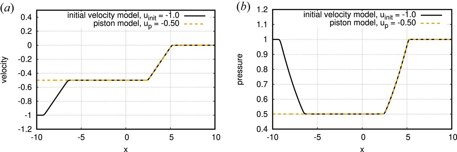
 $u_\mathrm {init}$ is the initial disturbance parameter introduced in § 2.2. The equivalence of the two models can be clearly seen in figure 4, where mirror symmetric forward and backward rarefaction waves are shown as the solid line, and the dashed line denotes the analytic solution given in (3.1)–(3.3).
Results of the numerical simulation of the initial velocity model (solid line) compared with the exact solution of the equivalent piston model (dashed line). The plots shown are for (a) velocity and (b) pressure at time  $t = 4.0$.

Figure 4 shows the comparison of piston model in 1-D theory (Chao et al. Reference Chao, Kan, Lui and Akasofu1977) and the 1-D simulation of the initial velocity model with a grid density of 128 points per unit length. There is an excellent agreement between the results, confirming the equivalence of the two models.
3.2. 2-D gas model
In the previous section, of the three plasma parameters defined earlier, we used only the initial velocity,  $u_\mathrm {init}$. We now extend the non-magnetized plasma model to 2-D by adding (so far unmagnetized) north and south ‘lobe’ regions. This introduces the second parameter, sheet/lobe temperature ratio
 $\tau$. Since the lobe magnetic field is zero, the pressure balance is achieved by making the initial pressure uniform over the entire simulation area.
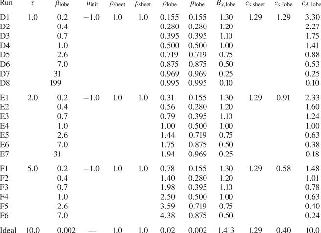
The initial conditions for simulation runs A, B and C are shown in table 2, where variables  $X_\mathrm {sheet}$ are for the plasma sheet (
 $\boldsymbol {U}_\mathrm {L}$,
 $\boldsymbol {U}_\mathrm {R}$) and variables
 $X_\mathrm {lobe}$ are for the magnetic lobes (
 $\boldsymbol {U}_\mathrm {D}$,
 $\boldsymbol {U}_\mathrm {U}$). The magnetic fields are all set to zero,
 $\boldsymbol {B}_\mathrm {sheet} = \boldsymbol {B}_\mathrm {lobe} = \boldsymbol {0}$. Each of these configurations was simulated with initial disturbance
 $\boldsymbol {U}_\mathrm {L}$, with velocity
 $u_\mathrm {init} = -1.0$.
Initial conditions for the 2-D unmagnetized plasma simulations.

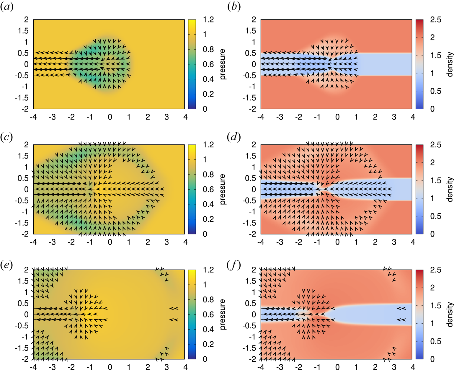
The 2-D plots of density for run B ( $\tau = 2.0$,
 $u_\mathrm {init} = -1.0$) are given in figure 5. At time
 $t = 0$, the left half of the plasma sheet (
 $x < 0$,
 $-0.5 < y < 0.5$) begins moving to the left at velocity
 $u_\mathrm {init}$. This creates a drop in pressure in the centre of the plasma sheet, which starts pulling in the surrounding plasma. As a result, a rarefaction wave starts spreading in all directions. The plasma from the right half of the sheet is pulled by the rarefaction wave, lowering pressure and breaking the balance between sheet and lobes.
Plots of pressure and density evolution for run B ( $\tau = 2.0$,
 $u_\mathrm {init} = -1.0$) of the 2-D gas simulation with a grid resolution of 32 points per unit length. After an initial set-up period, the thinning does not propagate tailward. Velocity vectors are over-plotted, at a resolution of four vectors per unit length, with velocities below
 $0.075$ not shown for clarity. Density plots are shown because the shape of the plasma sheet is not visible in the pressure plots, as the initial pressure is uniform. (a) Pressure at
 $t = 1.0$, (b) density at
 $t = 1.0$, (c) pressure at
 $t = 2.5$, (d) density at
 $t = 2.5$, (e) pressure at
 $t = 4.0$, (f) density at
 $t = 4.0$.

As the pressure balance is disturbed, lobe plasma starts pushing at the sheet plasma, transforming the rarefaction wave into plasma sheet thinning (figure 5b). However, due to the inward movement of the lobe plasma, the sheet plasma is compressed, its pressure rises, and the pressure balance between sheet and lobes is quickly re-established. While the rarefaction wave itself continues to propagate in all directions, since the jump between sheet and lobe pressures is lost, there is no further significant inward movement of the sheet–lobe boundary on the right-hand side ( $x > 0$) after
 $t \gtrsim 2.5$ (figure 5d,f).
As can be seen from table 2, initial properties of sheet and lobe plasmas for run A are identical. As a result, the rarefaction wave generated by the initial velocity spreads evenly in all directions, and since there is no distinct sheet–lobe boundary, no thinning can be observed.
In run C, the deformation of the boundary progresses through the identical sequence as in run B. However, the development is slightly slower, presumably due to a lower sound velocity in the lobes.
4. Plasma model, simulation and results
Finally, we introduce the lobe magnetic field, described with the third parameter, lobe plasma beta  $\beta _\mathrm {lobe}$. A realistic lobe plasma beta would be of the order of
 $\beta _\mathrm {lobe} \lesssim 0.01$ (Baumjohann, Paschmann & Lühr Reference Baumjohann, Paschmann and Lühr1990); however, this is difficult to achieve in a simulation due to the extremely low kinetic pressure in such a plasma. For this paper, we limit the values of plasma beta to
 $\beta _\mathrm {lobe} \geqslant 0.2$.
The addition of the magnetic field to the lobe plasma means that, to keep the total pressure constant and the lobe/sheet pressure balanced, the lobe kinetic pressure must be lowered. An overview of the initial conditions is shown in table 3.
An overview of the initial conditions for 2-D plasma sheet simulations. The last row shows the ideal, realistic values, which could not be used due to limitations of the simulation program.

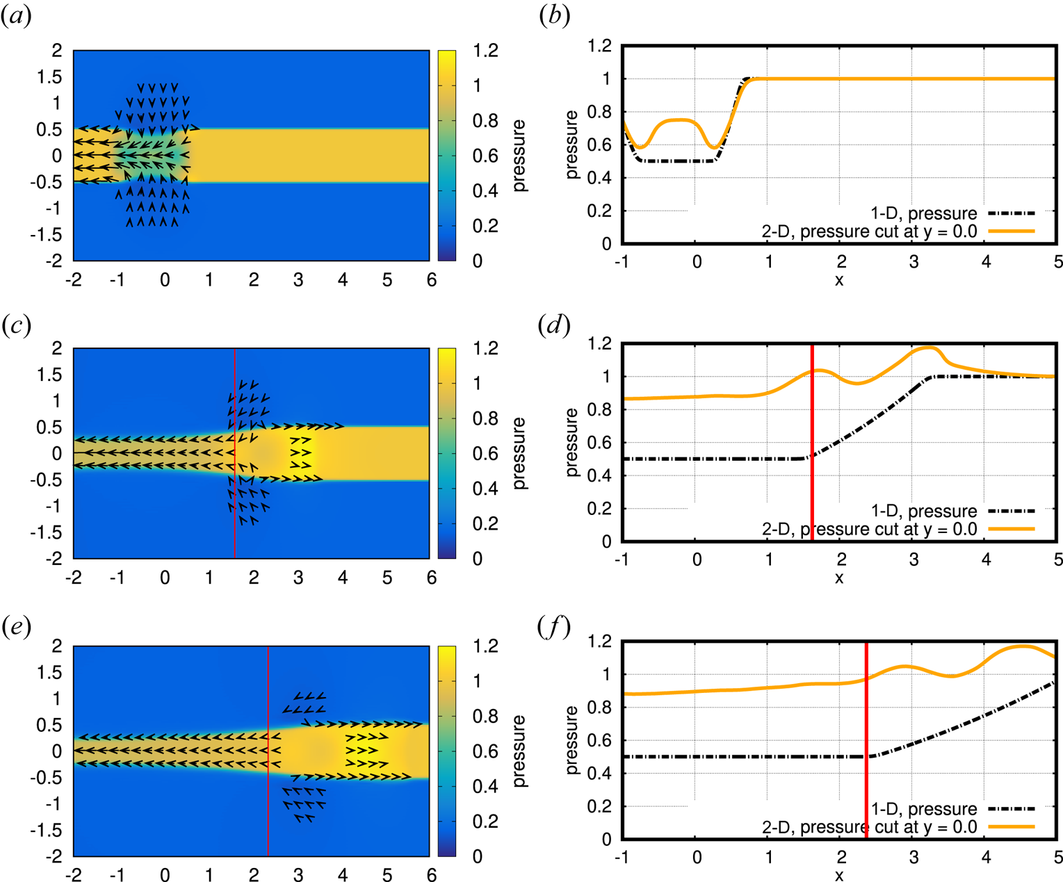
Two-dimensional plots of pressure for run E1 are shown on the left side of figure 6. At time  $t = 0$, the left half of the plasma sheet begins moving earthward. The pressure drop that the disturbance leaves behind pulls in the surrounding plasma (figure 6a). The right side of figure 6 shows the time evolution of sheet pressure taken from 1-D gas simulation at a grid density of 128 points (black dash-dotted line) and a profile at
 $y = 0$ taken from the 2-D plasma simulation (orange solid line). For a few moments, the resulting rarefaction wave in two dimensions is similar to the one in the 1-D simulation (
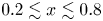 $0.2 \lesssim x \lesssim 0.8$ in figure 6b); however, as the boundaries with the magnetic lobes move inward due to loss of the pressure balance, the plasma sheet is compressed and the pressure rises, nullifying the rarefaction wave and generating a wave train of pulses of increased pressure (figure 6d,f). The produced waves will be identified as fast-mode MHD waves in § 5. Despite the apparent loss of the rarefaction wave, the earthward plasma flow and the accompanying thinning of the plasma sheet continue. It is noted that the thinning propagates in a self-similar fashion after an initial set-up period at
 $t \lesssim 1$ (see figure 6c,e).
Plots of pressure evolution for run E1 ( $\tau = 2.0, \beta _\mathrm {lobe} = 0.2, u_\mathrm {init} = -1.0$) of the 2-D plasma simulation with a resolution of 32 grid points per unit length. Panel (a) shows the initial plasma sheet pressure drop and the beginning of recompression. Panels (c,e) show the propagation of the thinning front, with the detected location of the front marked with a red line. Velocity vectors are over-plotted, at a resolution of four vectors per unit length, with velocities below
 $0.075$ not shown for clarity. Panels (b), (d) and (f) show the comparison of pressure in 1-D and 2-D simulation, with the detected location of the front again marked with a red line. The grid density for 1-D simulation is 128 points per unit length. For the 2-D simulation, we show the horizontal cut through the centre of the plasma sheet, at
 $y = 0$. (Note that it is only a coincidence that the thinning front and the foot of the 1-D rarefaction wave are in approximately the same location. Since the sheet parameters do not change the 1-D rarefaction wave is identical in all of the simulation runs, while the location of the thinning front is different for each run.) (a) Pressure at
 $t = 0.5$, (b) 1-D versus 2-D at
 $t = 0.5$, (c) pressure at
 $t = 2.5$, (d) 1-D versus 2-D at
 $t = 2.5$, (e) pressure at
 $t = 4.0$, (f) 1-D versus 2-D at
 $t = 4.0$.

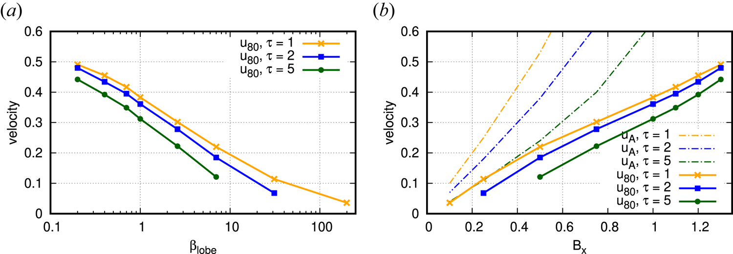
The other runs listed in table 3 follow the same basic sequence of events, albeit with different propagation velocities and thinning amounts; the propagation velocity decreases as lobe beta and temperature ratio  $\tau$ increase. While the propagation velocity appears to be fairly constant over a single simulation run for sufficiently large
 $\beta$, for lobe plasmas with
 $\beta \gg 1$ the measured propagation velocity may eventually stop or even slightly reverse direction. This effect is more pronounced in runs with higher temperature ratio
 $\tau$, where sound and Alfvén velocities in the lobe are lower. Presumably, the physical process that causes the propagation of the thinning front is on too slow a time scale for the current simulation. As the actual lobe plasma has
 $\beta \ll 1$, and the high-beta simulations have been conducted only to determine the overall scaling and confirm it asymptotes towards the ‘infinite-beta’ gas simulation from § 3, the affected runs are not required and have been discarded from the overview table and the following analysis.
It is worth noting that we observed the development of Kelvin–Helmholtz instability on the sheet–lobe interface, arising due to the velocity difference between the two plasmas (Chandrasekhar Reference Chandrasekhar1981). However, the instability appears only for the weak magnetic field ( $B_{x, \mathrm {lobe}} \lesssim 0.5$,
 $\beta _\mathrm {lobe} \gtrsim 7$), and when it does appear its effect is constrained to the far left of the simulation domain (
 $x \lesssim -3$), where the velocity difference is significantly larger. As we are only interested in the right-hand side of the domain (
 $x > 0$), the presence of the instability does not affect the following discussions.
Additionally, the flows that can be seen on the sheet–lobe boundary in the right-hand half of figure 6(c,e) are due to thin, non-physical jets in the two-grid-points-wide transition area between sheet and lobe, which was introduced to increase the numerical stability of the simulation by slightly smoothing out the initial discontinuity. Increasing the grid density and/or widening the transition area weakens the jets; however, as widening the transition area makes the following analysis more difficult, and the evolution of the plasma sheet shape does not noticeably change, we kept the transition area width at two grid points.
For further analysis of the plasma sheet thinning, we measure the propagation velocity of its front with the following method. First, for each discrete  $x$ coordinate, we linearly interpolate the
 $B_x$ profile to find the location in
 $y$ where the magnetic field drops below half of the initial lobe value. Collecting all the
 $(x,y)$ values gives us a rough profile of the plasma sheet, which we can again linearly interpolate to obtain the
 $x$ coordinate of the point where the sheet thickness is reduced to
 $80\,\%$ of the initial value. We repeat the procedure and obtain the ‘
 $80\,\%$ thinning’ locations between
 $t = 2$ and
 $t = 10$ (skipping the initial period at
 $t < 2.0$ where the self-similar shape of the thinning may not yet be fully developed). Finally, we derive the thinning velocity
 $u_{80}$ from a linear fit on the ‘
 $80\,\%$ thinning’ locations. The results for grid density
 $32$ are shown in figure 7.
Front velocity dependence on the temperature ratio  $\tau$ and the plasma beta
 $\beta _\mathrm {lobe}$ (a) for 2-D simulations with grid density of 32 points, plotted versus lobe beta (a) and the initial lobe magnetic field strength (b) with Alfvén velocities for the lobe initial conditions shown for comparison. The relationship between lobe beta and lobe magnetic field is
 $\beta _\mathrm {lobe} = 2/B_x^2 - 1$.

We can observe a strong, approximately linear dependence between the magnetic field strength in the lobes and the thinning velocity. Furthermore, all thinning velocities are considerably slower than the sheet sound velocity. Assuming the linear relationship holds for smaller  $\beta _\mathrm {lobe}$ (larger
 $B_{x,\mathrm {lobe}}$), and taking into account that, in order to satisfy the pressure balance condition (2.7),
 $B_{x,\mathrm {lobe}} \leqslant \sqrt {2}$, we can extrapolate that the maximum velocity of the
 $80\,\%$ thinning is
 $u_{80} \sim 0.5$, or less than half of the sheet sound velocity
 $c_{s,\textrm {sheet}} = 1.29$.
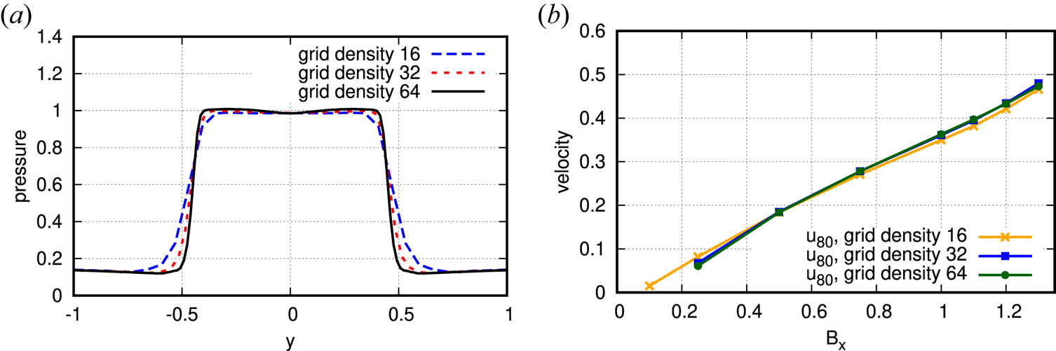
In order to show numerical convergence, the comparison between grid densities for temperature ratio  $\tau = 2$ is shown in figure 8. We can see a good agreement between grid densities
 $16$ and
 $32$, and an excellent agreement between grid densities
 $32$ and
 $64$. More specifically, for
 $\beta _\mathrm {lobe} \leqslant 7$ (
 $B_{x,\mathrm {lobe}} > 0.5$), the disagreement in thinning velocity between grid densities
 $16$ and
 $32$ is below
 $4\,\%$, and the disagreement between grid densities
 $32$ and
 $64$ is below
 $2\,\%$. The convergence worsens for
 $\beta _\mathrm {lobe} > 7$, as determining the thinning velocity grows less reliable and requires more grid density as that velocity nears zero. However, lobe plasma is a low-beta plasma, and the simulations for
 $\beta _\mathrm {lobe} > 1$ are used only to confirm that the thinning velocity goes to zero as lobe beta rises (as anticipated from the 2-D gas simulation); therefore, somewhat rough results for high values of lobe beta are acceptable.
Comparisons between simulation results with different grid densities. Pressure profiles of the plasma sheet are increasingly smeared out as grid density falls (a), though the sheet width is consistent. The impact of the minor width variation on measured thinning velocity is low (b). (a) Pressure profiles for run E1 at  $x = 2.0$. (b) Thinning velocity versus
 $B_x$.

5. Wave decomposition
One possible approach that can be used to determine the physical process behind an event in a system of conservation laws is to decompose the disturbances into component waves. The decomposition may be obtained by applying a diagonalization procedure similar to the one presented by Shu (Reference Shu1998).
Each  $x$ and
 $y$ coordinate of the 2-D system is, again, treated as a collection of 1-D systems of the form
 \begin{equation} \frac{\partial \boldsymbol{U}}{\partial t} + \frac{\partial }{\partial x}\boldsymbol{F}(\boldsymbol{U}) = 0, \end{equation}
and an equivalent system in the  $y$ direction. Multiplying from the left with the matrix
 $\boldsymbol{\mathsf{L}} = (\boldsymbol {L}_1, \ldots , \boldsymbol {L}_n)$, where
 $\boldsymbol {L}_1, \ldots , \boldsymbol {L}_n$ are the left eigenvectors of the system's Jacobian,
 $\partial \boldsymbol {F} / \partial \boldsymbol {U}$, and assuming the matrix
 $\boldsymbol{\mathsf{L}}$ is constant, we obtain a diagonalized system
 \begin{equation} \frac{\partial (\boldsymbol{\mathsf{L}} \boldsymbol{U})}{\partial t} + \frac{\partial (\boldsymbol{\mathsf{L}} \boldsymbol{F})}{\partial x} = 0, \end{equation}
which can be split into a set of  $n$ independent advection equations
 \begin{equation} \frac{\partial w_i}{\partial t} + \lambda_i \frac{\partial w_i}{\partial x} = 0, \end{equation}
where  $w_i$
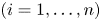 $(i = 1, \ldots , n)$ is a component of the transformed vector
 $\boldsymbol {W} = \boldsymbol{\mathsf{L}} \boldsymbol {U}$ and
 $\lambda _i$ are the respective eigenvalues corresponding to
 $\boldsymbol {L}_i$. It follows that an approximate strength of each wave component can be calculated by discretizing the transformed flux
 $\boldsymbol{\mathsf{L}}\boldsymbol {F}$ from (5.2). Unfortunately, in the case of MHD the matrix
 $\boldsymbol{\mathsf{L}}$ is not constant; however, by locally freezing the value of
 $\boldsymbol{\mathsf{L}}$, we may still obtain an approximate decomposition.
We define the strength of wave components  $\boldsymbol {S}_{j+1/2}$ between grid points
 $j$ and
 $j+1$ as
 \begin{equation} \boldsymbol{S}_{j+1/2} = \boldsymbol{\mathsf{L}}_{j+1/2} \boldsymbol{F}_{j+1} - \boldsymbol{\mathsf{L}}_{j+1/2} \boldsymbol{F}_{j}, \end{equation}
where  $\boldsymbol{\mathsf{L}}_{j+1/2} = \boldsymbol{\mathsf{L}}(\boldsymbol {U}_{j+1/2})$ is the discretized value of the matrix of the left eigenvectors
 $\boldsymbol{\mathsf{L}}$ between grid points
 $j$ and
 $j+1$, with
 $\boldsymbol {U}_{j+1/2}$ calculated by averaging density, velocity, magnetic field and total pressure of
 $\boldsymbol {U}_{j}$ and
 $\boldsymbol {U}_{j+1}$ (Brio & Wu Reference Brio and Wu1988) and
 $\boldsymbol {F}_{j} = \boldsymbol {F}(\boldsymbol {U}_{j})$ is the discretized flux at grid point
 $j$.
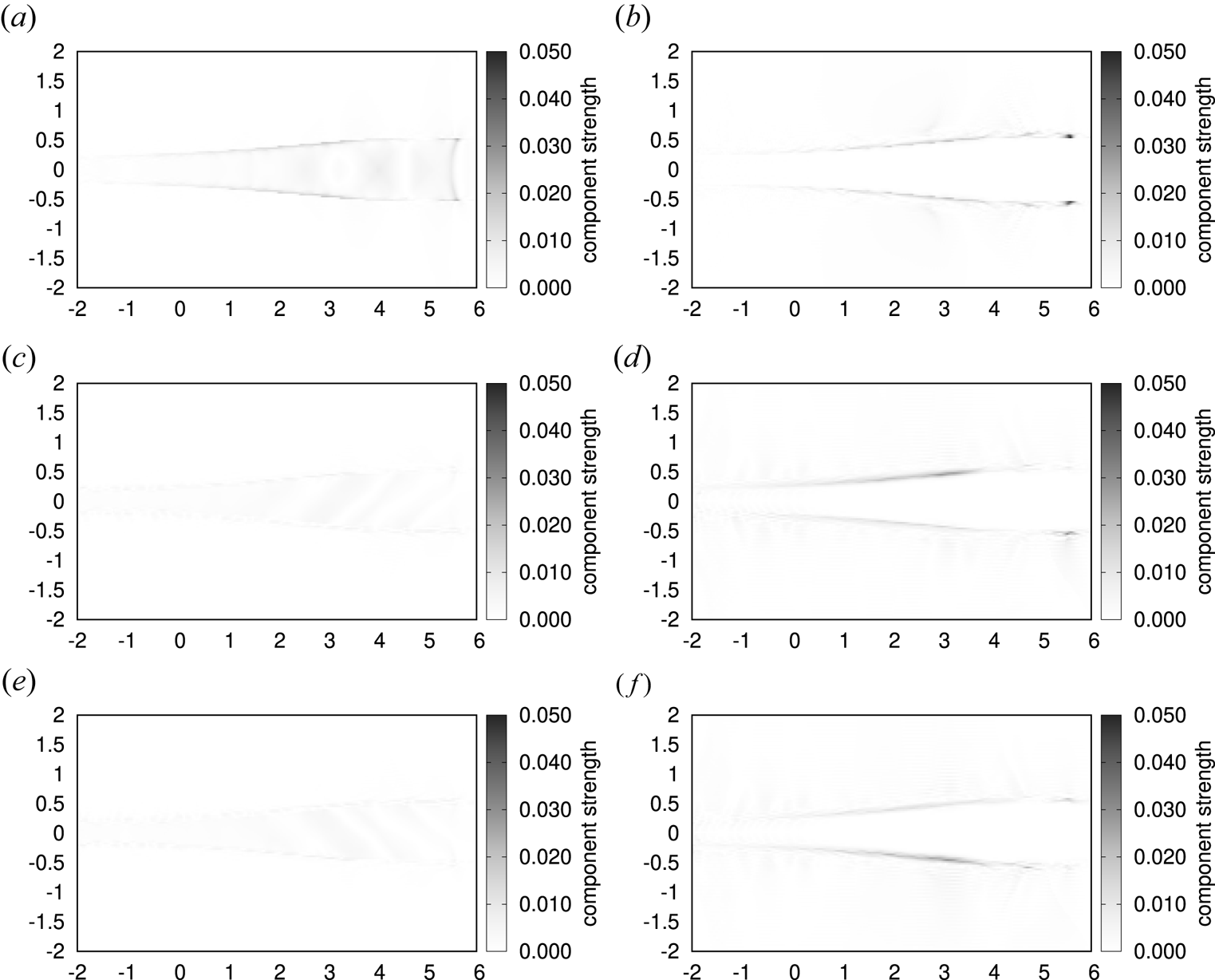
Figure 9 shows the dominant wave components  $|\boldsymbol {S}_{j+1/2}|$ in the
 $x$ and
 $y$ directions around the thinning front of the plasma sheet for run E1, with other components being at most half as large as the maximum of the positive-direction fast-mode component (
 $\approx 0.025$), which is half as large as the peaks of the slow-mode component (
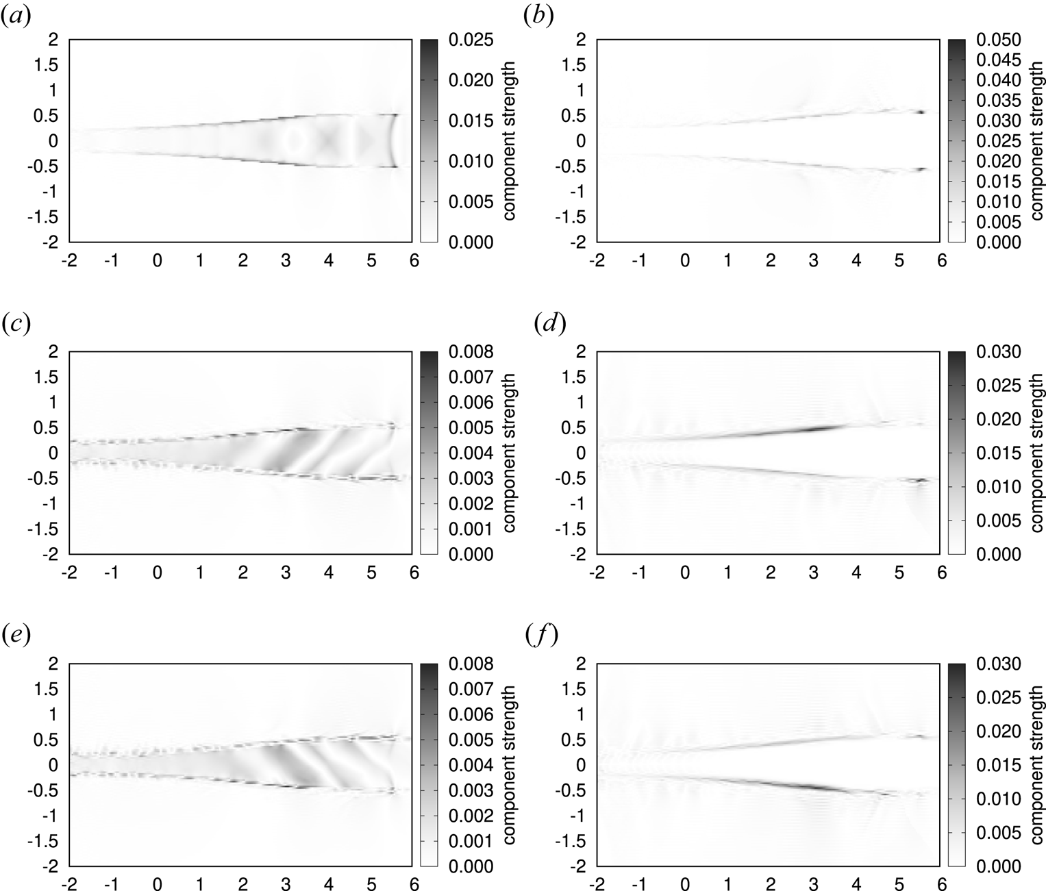
 ${\approx }0.050$). Figure 10 shows the same components, rescaled to better show their structure.
Absolute value of the wave strengths  $|\boldsymbol {S}_{i+1/2}|$ at time
 $t = 4.0$ for run E1 (
 $\tau = 2.0$,
 $\beta _\mathrm {lobe} = 0.2$,
 $u_\mathrm {init} = -1.0$) of the 2-D plasma simulation with a resolution of 32 grid points per unit length. All plots are scaled to the same value to allow for relative comparison; see figure 10 for clearer representation of individual plots. (a) Fast-mode wave in the positive
 $x$ direction, (b) slow-mode wave in the positive
 $x$ direction, (c) fast-mode wave in the negative
 $y$ direction, (d) slow-mode wave in the negative
 $y$ direction, (e) fast-mode wave in the positive
 $y$ direction, (f) slow-mode wave in the positive
 $y$ direction.

Absolute value of the wave strengths  $|\boldsymbol {S}_{i+1/2}|$ at time
 $t = 4.0$ for run E1 (
 $\tau = 2.0$,
 $\beta _\mathrm {lobe} = 0.2$,
 $u_\mathrm {init} = -1.0$) of the 2-D plasma simulation with a resolution of 32 grid points per unit length. All plots are scaled to their own maximum value; see figure 9 for comparison between different wave modes. (a) Fast-mode wave in the positive
 $x$ direction, (b) slow-mode wave in the positive
 $x$ direction, (c) fast-mode wave in the negative
 $y$ direction, (d) slow-mode wave in the negative
 $y$ direction, (e) fast-mode wave in the positive
 $y$ direction, (f) slow-mode wave in the positive
 $y$ direction.

A wave train of fast-mode MHD waves (i.e. sound waves) propagating tailward at sound velocity can be observed inside of the plasma sheet in figure 10(a), with peaks and troughs that roughly align with, respectively, troughs and peaks of pressure in figure 6(f). There also appears to be a slow-mode MHD wave propagating in the  $x$ direction along the sheet–lobe boundary, visible as a peak at
 $(x,y) \approx (5.6, \pm 0.5)$ in figure 10(b). However, the slow-mode peak is not moving at the lobe slow magnetosonic speed of
 $0.91$, but instead moves at the sheet fast magnetosonic speed (i.e. sound speed) of
 $1.29$, advancing together with the dark arc-like structure at the front of the plasma sheet wave train at
 $x \approx 5.5$. Since there is a sharp change at the exact point of the sheet–lobe interface when crossing between sheet and lobe, where the fast-mode component (the dark arc) suddenly weakens and the slow-mode component (the peaks) grows, it is likely that the slow wave is generated through mode conversion by the front of the fast-mode wave-train as it touches the boundary.
From the decomposition in the  $y$ direction, in figure 10(d,f) we can observe a strong slow-mode component along the sheet–lobe boundary when crossing from lobe to sheet. As the plasma changes from the strongly magnetized lobe plasma into non-magnetized sheet plasma, the slow magnetosonic speed falls to zero and the slow wave at the boundary is unable to enter the sheet. Instead, it appears to launch a series of fast-mode waves across the sheet, clearly visible in figure 10(c,e). The location of the peak of the
 $y$ direction slow-mode wave corresponds to the thinning front of the plasma sheet, suggesting that the slow-mode wave may be driving the thinning process.
Comparing figure 10 with the pressure plots in figure 6, we can see that, while the  $x$ direction wave train moves at the same velocity as the rarefaction wave in the 1-D model, it causes the sheet pressure to increase instead of decrease, resisting the deformation of the magnetic field lines. After the pulses of increased pressure associated with the wave train pass, the sheet–lobe boundary starts moving inward and the thinning begins, as can be seen from the
 $y$ direction slow-mode MHD waves in figure 10(d,f). The wave train appears to be influenced by the slow-mode wave at the sheet–lobe boundary; as the
 $y$ direction fast-mode waves move across the sheet, new waves are generated slightly tailwards, giving the appearance of a right-moving stripe. The first pulse in the wave train is generated during the initial sheet recompression, as can be seen in figure 6(b).
It is worth noting that there were no Alfvén waves detected by the wave decomposition procedure, down to the level of the numerical error. This suggests that the  $y$ direction slow-mode waves are the primary driver behind the bending of the magnetic field lines during the thinning process.
6. Comparison of 1-D and 2-D models
In the 1-D gas model (Chao et al. Reference Chao, Kan, Lui and Akasofu1977), the initial disturbance generates a rarefaction wave travelling tailward. As the pressure drops behind the wave, the boundary between sheet and lobe is forced to move inward. Since the plasma beta in the sheet is greater than one, the rarefaction wave moves at the sound velocity,  $c_{s,\textrm {sheet}}$. The thinning front, presumably, moves at approximately the same velocity. There is no stated dependence between the thinning front velocity and the conditions in the magnetic lobes; only the thinning amount is influenced by them.
Extending to a 2-D gas model, we observed that the rarefaction wave generated by the initial disturbance is drastically weakened in the first moments of the event. Furthermore, even though this weakened form of the rarefaction wave continues propagating, the thinning ceases to propagate due to the loss of the sheet–lobe pressure difference (see figure 5).
Extending to a 2-D plasma model by introducing the magnetic field into the lobes, the dynamics of the plasma sheet thinning drastically changes.
Firstly, the rarefaction wave is weakened so much that it is no longer clearly noticeable as an independent entity. It is either subsumed in other, stronger waves, or completely extinguished by compression in the first few moments of the event. In either case, the significant drop in pressure ceases to propagate tailward. However, despite the lack of a significant pressure drop, and in stark contrast to the 2-D gas model, the thinning continues to propagate (figure 6). This indicates that the rarefaction wave is not a sole component of the plasma sheet thinning.
Secondly, the thinning front velocity is lower than the rarefaction wave velocity. This is another indicator that thinning dynamics have separated from the rarefaction wave that initially caused them.
Thirdly, the thinning front velocity shows a strong dependence on the conditions in the magnetic lobes (figure 7). The thinning front propagates faster when the lobe magnetic field is stronger, in stark contrast to the 1-D model. As the 2-D gas simulation showed, in the limit of no magnetic field there is an initial burst after which the thinning front completely stops propagating; this aligns with the small  $B_x$ limit of the 2-D plasma simulation.
Fourthly, in the 2-D plasma model there is a wave train of slight pressure increases moving tailward through the plasma sheet at the fast magnetosonic (i.e. sound) velocity (figure 6). The wave train is completely absent in the 1-D and 2-D gas models.
The above points of comparison clearly show that the dynamics of plasma sheet thinning seem to be dominated by the sheet–lobe interaction that could not be accounted for in the 1-D model.
Finally, as mentioned in § 1, the CD model employs the rarefaction wave and the resulting pressure drop to trigger reconnection in the near Earth neutral line. That is, the rarefaction wave needs to propagate tailward for a long distance, for example, from the site of CD ( ${\sim } -10 R_{e}$) to that of reconnection (
 ${\sim }-20 R_{e}$), which are approximately
 $10 R_{e}$ apart. In the current simulation study, however, the rarefaction wave and, more importantly, corresponding pressure drop are damped soon after the occurrence of pressure decrease due to CD. Therefore, the mechanism described in the CD model may be insufficient to trigger reconnection because of the weakening of pressure decrease in the central plasma sheet at
 ${\sim } -20 R_{e}$. In this sense, the results of the numerical simulation suggest that the CD model may need to be carefully reconsidered to account for magnetic reconnection, as the current form may not be able to fully explain all the phenomena in the magnetotail during the episode of auroral substorm.
7. Conclusion
Starting from a simple 1-D model of the plasma sheet thinning, we have first extended it to a 2-D configuration by adding the north and south (non-magnetic) lobes. In this 2-D gas simulation the rarefaction wave is weakened and thinning ceases to propagate (figure 5). After adding a magnetic field to the lobes and simulating the resulting 2-D plasma model, we observed that the thinning propagates again, but this time the rarefaction wave is absent (figure 6).
The lack of thinning propagation in the 2-D gas simulation means that the influence of the sheet–lobe configuration on the dynamics can be too strong to allow extrapolating the behaviour from a 1-D model. The appearance of thinning in the 2-D plasma simulation indicates that the deformation of the magnetic field may play a significant role in the plasma sheet thinning. This conclusion is strengthened by observing that the signature aspect of the CD model of the plasma breakup, the rarefaction wave, as well as its associated pressure drop, are drastically weakened soon after the event begins, and the thinning, which was supposed to be following behind the – now absent – rarefaction wave, continues propagating, though at a slower velocity. The thinning is preceded by a wave train of pulses of increased pressure, propagating tailward as fast-mode MHD waves. The thinning begins after the wave train passes, and its velocity is shown to be strongly influenced by the conditions in the magnetic lobes; in particular, there is an approximately linear dependence on the lobe magnetic field strength.
Finally, the weakening or outright disappearance of the rarefaction wave and the presence of the wave train indicate that it is possible that the reconnection in the CD model may not be preceded by a significant drop in pressure. While a relatively small pressure drop is still present (figure 6f), it is preceded by pulses of pressure increase in the centre of the plasma sheet, and the thinning front appears to be positioned ahead of the pressure drop.
However, the ideal MHD model employed in the simulation is unable to reproduce the magnetic reconnection, and therefore does not address the development of the system after the thinning of the plasma sheet. It may be that the aforementioned weakened drop in pressure is still sufficient to trigger the reconnection when finite resistivity or non-MHD effects are included. A more sophisticated simulation model, e.g. the extended MHD or a kinetic model, would be required to determine whether the reconnection ultimately does or does not occur under the simplified geometry used in this paper.
In future research, we hope to more precisely determine the dependence of the plasma sheet thinning on the parameters of the plasma sheet and magnetic lobes. We would also like to confirm whether or not the reconnection can occur if the presented plasma sheet configuration is simulated with a more sophisticated simulation model.
Acknowledgements
We thank Dr. Takashi Minoshima of the Japan Agency for Marine-Earth Science and Technology (JAMSTEC) for valuable discussions. This research was partially supported by the Rotary Yoneyama Memorial Scholarship.
Editor William Dorland thanks the referees for their advice in evaluating this article.
Declaration of interests
The authors report no conflict of interest.