


1. Introduction
The strong conditions that supported U.S. wineries in 2020 and 2021 have given way to pronounced strain. Demand has softened—reflected in declining direct-to-consumer shipments and demographic turnover that raises doubts about whether younger consumers will replace older cohorts at comparable rates—while production risk from wildfires and smoke taint has increased (Kwok and Lee, Reference Kwok and Lee2026; McMillan, Reference McMillan2026). The California Association of Winegrape Growers is now recommending that 30,000–50,000 acres of vineyards be pulled out of production—roughly the entire wine grape acreage of Washington State (Martine, Reference Martine2025). These pressures have compressed margins and heightened uncertainty in an industry where location, production practices, and product quality are closely linked.
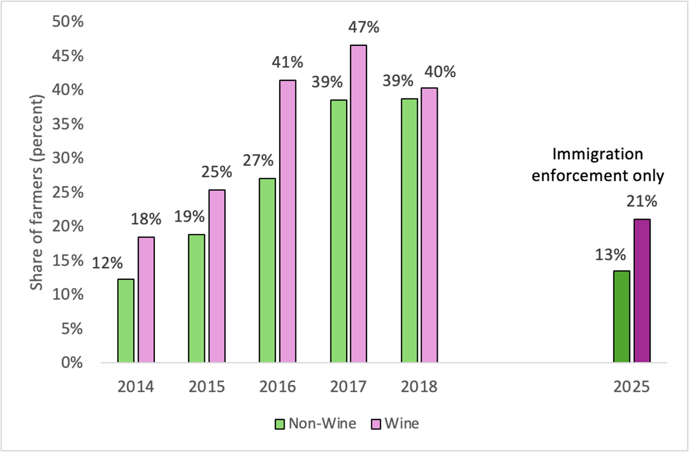
Compounding these conditions is a tightening labor supply, as illustrated in Figure 1. Recent evidence from a broad cross-section of California agriculture documents widespread labor shortages and a range of producer responses, including wage increases, changes in cultivation practices, adoption of labor-saving technologies, and adjustments to labor arrangements (Win et al., Reference Win, Rutledge and Maredia2025). Wine growers reported consistently higher rates of labor shortage than other California farmers over 2014–2018, with the gap widening as overall shortages increased. Immigration enforcement has since introduced an additional source of disruption: 21% of wine growers report enforcement-induced labor loss in 2025, compared to 13% of non-wine growers. Such shocks reduce worker participation directly rather than through wages and may therefore be difficult to offset through higher pay or expanded recruitment (Rutledge and Win, Reference Rutledge and Win2026).
Trend of labor shortages (2014–2018) and enforcement-induced labor loss (2025).

Labor supply constraints may have particularly consequential effects in wine grape production. Vineyard management involves a sequence of labor-intensive, time-sensitive operations that require experienced crews, must be completed within narrow windows, and directly affect grape development and final product characteristics. In premium regions, manual practices are closely tied to product differentiation and price. As a result, labor disruptions affect not only production costs but also realized output and quality and may be more difficult to offset through substitution than in other agricultural settings.
Labor shortages in specialty crop agriculture are well documented, but the issue has received little direct attention in wine economics, where labor is arguably most difficult to substitute. Farmers across U.S. specialty crops have reported persistent difficulty securing sufficient workers for more than a decade (Glaister, Reference Glaister2006; Plummer, Reference Plummer2013; CFBF and UC Davis, 2019; della Cava and Lopez, Reference della Cava and Lopez2019; Estrabrook, Reference Estrabrook2021). Research has documented the extent of these shortages (Martin, Reference Martin2007; Hertz and Zahniser, Reference Hertz and Zahniser2012; Richards, Reference Richards2018), examined their drivers (Richards and Patterson, Reference Richards and Patterson1998; Boucher et al., Reference Boucher, Smith and Taylor2007; Taylor et al., Reference Taylor, Charlton and Yúnez-Naude2012; Kostandini et al., Reference Kostandini, Mykerezi and Escalante2013; Fan et al., Reference Fan, Gabbard, Pena and Perloff2015; Charlton and Taylor, Reference Charlton and Taylor2016), and evaluated mitigation strategies (Taylor et al., Reference Taylor, Charlton and Yúnez-Naude2012; Richards, Reference Richards2018, Reference Richards2020; Zahniser et al., Reference Zahniser, Taylor, Hertz and Charlton2018; Charlton et al., Reference Charlton, Taylor, Vougioukas and Rutledge2019; Hamilton et al., Reference Hamilton, Richards, Shafran and Vasilaky2021). The weight of evidence indicates that agricultural labor has become persistently scarcer (Taylor et al., Reference Taylor, Charlton and Yúnez-Naude2012; Charlton and Taylor, Reference Charlton and Taylor2016; Richards, Reference Richards2018). Labor constraints have been reported in major wine-producing regions outside the United States as well (Mansuri, Reference Mansuri2023; Wine Australia, 2024). Yet labor appears only indirectly in existing work in wine economics: through historical labor institutions (Fourie and Greyling, Reference Fourie and Greyling2023), clustering choices (Fouad and Scott III, Reference Fouad and Scott2024), or measures of productivity (Žiković et al., Reference Zikovic, Katunar and Višić2025). This gap is notable given how central labor is to high-value wine grape production.
In this paper, we examine how labor shortages affect production decisions and outcomes in the wine grape sector. We argue that wine production offers limited scope for adjustment when labor becomes scarce, particularly in settings where quality-sensitive operations, long-lived vineyard capital, and terrain constraints restrict substitution.
To assess these limits, we exploit two distinct sources of labor disruption. The first captures gradual labor market tightening from 2014 to 2018, a setting in which growers can adjust over multiple seasons. The second isolates labor losses associated with immigration enforcement in 2025, a more sudden shock that is less likely to be offset through conventional margins such as wage increases or recruitment. Comparing responses across these settings allows us to examine how adjustment varies with the nature of the labor shock.
Our analysis draws on original survey data collected in collaboration with the California Farm Bureau, covering a broad cross-section of California producers and providing detailed information on labor shortages, operational adjustments, and production responses. Summary results for the full sample of California farmers have been reported elsewhere (Win et al., Reference Win, Rutledge and Maredia2025; Rutledge and Win, Reference Rutledge and Win2026); here, we focus on wine grape producers and comparisons across crops and regions.
Using these data, we document three main findings. First, in the period of gradual labor market tightening, wine grape producers adjust primarily through wage increases and cultivation practice changes, with little use of technology or acreage reduction relative to other farmers. Second, in premium regions, adjustment shifts toward farm labor contractors (FLCs) and cultivation changes, with no evidence of technology adoption or scale reduction, consistent with tighter specialized labor markets and limited scope for substitution. Third, when labor disruptions reflect immigration enforcement, adjustment becomes more limited, with production reduction emerging as the primary response and little evidence of adjustment along other margins. Mechanism tests indicate that these patterns are not explained by general crop labor intensity alone, pointing to structural features of wine production as an independent source of constraint.
The findings contribute to the literature on agricultural labor shortages by documenting heterogeneity in adjustment margins across crops and showing how production characteristics shape responses to input scarcity. Within the economics of wine, they identify labor availability as a central constraint on production in high-value regions, a dimension that has received little direct attention despite its importance for understanding costs, output, and quality. More broadly, the results illustrate that labor market shocks may affect not only costs but also realized production in sectors where labor is difficult to substitute.
2. Institutional background
2.1. Labor in U.S. wine production
Grape production in California is characterized by substantial heterogeneity in production values across varieties and growing regions (Sambucci and Alston, Reference Sambucci and Alston2017), and its reliance on manual labor likewise varies across regions and quality tiers. In premium segments, skilled manual labor is central throughout the production cycle. Pruning, canopy management, thinning, and harvest must each be completed within narrow time windows and often require crop- and site-specific skill. Many high-value vineyards are located on hillside terrain that limits or precludes mechanization.
These features shape labor demand in predictable ways. Vineyard operations generate short periods of concentrated demand, particularly at harvest. Because the timing and execution of these tasks directly affect output quality, the scope for substituting other inputs is limited. Delays or errors can reduce both yields and prices in ways that are difficult to reverse.
In lower-value, volume-oriented production, mechanization plays a larger role. Regions such as Lodi rely extensively on mechanical harvesting, pruning, and sorting, supported by vineyard layouts—trellising, spacing, row orientation—designed to accommodate machinery. Per-acre labor requirements are correspondingly lower, though labor remains necessary throughout the production cycle.
Transitioning from manual to mechanical systems is not straightforward, even when economically attractive. Vineyards not designed for machine use require substantial modifications to trellising, spacing, and layout, and in some cases replanting. Because vineyard establishment involves large sunk costs and a multi-year period before full production, such adjustments are both expensive and slow. Consistent with these constraints, Franken (Reference Franken2014) shows that specialized and durable asset investments play an important role in the organization of the California wine grape supply chain, particularly where quality considerations are important. The scope for mechanization therefore depends in part on investment decisions made at establishment, which constrains the available responses to labor scarcity in the short and medium run.
Historically, labor needs have been met through direct hires, FLCs, and, to a lesser extent, H-2A guest workers. The availability of this workforce has become increasingly uncertain.
2.2. Enforcement actions and the “chilling effect”
Recent changes in immigration enforcement have introduced a distinct type of labor supply shock, one that operates primarily through behavioral responses among workers rather than through direct enforcement on farms. Several high-profile incidents illustrate the mechanism. In 2025, a high-profile vineyard manager in Oregon’s Willamette Valley was detained by federal immigration authorities while traveling to work (Figueroa, Reference Figueroa2025; The Guardian, 2025). Subsequent reporting described reduced worker mobility across employers and greater reluctance to travel to unfamiliar locations, even in the absence of further enforcement activity. Similar patterns have been reported in Sonoma County, where workers altered commuting behavior, avoided public spaces, and in some cases did not report to work, without direct enforcement on farms (Gray, Reference Gray2025; Mizuguchi, Reference Mizuguchi2025).
Survey evidence from California is consistent with these accounts (Rutledge and Win, Reference Rutledge and Win2026). Direct on-farm enforcement appears rare; fewer than 1% of wine grape growers report worker losses from farm-level enforcement actions. In contrast, approximately 20% report losses associated with general enforcement activity or worker anxiety. Roughly one-third of wine grape growers report at least one adverse outcome, including labor loss, operational disruption, or worker concern.
These patterns indicate that the primary channel is the broader enforcement environment rather than direct intervention. Perceived risk reduces effective labor supply by increasing absenteeism, limiting worker mobility, and disrupting established employment relationships, a mechanism commonly described as a “chilling effect.” Such shocks differ from gradual labor market tightening: they are sudden, difficult to anticipate, and less responsive to standard adjustments such as wage increases or formal recruitment.
2.3. Implications for wine production
Labor shocks may have distinct consequences in wine production, operating through three margins: acreage, input substitution, and timing.
Vineyard acreage adjusts slowly, reflecting high establishment costs and long investment horizons. Short-run responses to labor shortages therefore occur primarily through changes in labor use, production practices, or realized output rather than planted area.
Evidence from other shocks to California wine grape markets also points to substantial heterogeneity in growers’ supply responses across regions. Consoli et al. (Reference Consoli, Fraysse, Slipchenko, Wang, Amirebrahimi, Qin, Yazma and Lybbert2022), for example, find that the supply response to the Sideways-induced demand shock was concentrated in lower-value Central Valley vineyards, suggesting that adjustment margins can differ considerably across California wine-producing regions.
Substitution between labor and capital is imperfect, particularly in premium production. Many tasks in high-quality viticulture require skilled manual labor and cannot be readily mechanized, especially on the hillside sites characteristic of Napa and Sonoma. In lower-value regions with established mechanical systems, adjustment is more feasible, but even there labor cannot be eliminated.
Timing amplifies these constraints. Harvest and related operations must be completed within narrow windows; delays cause quality degradation that cannot be undone. Temporary labor shortfalls can therefore translate directly into lower output or reduced quality, not merely higher costs.
Over longer horizons, sustained labor uncertainty may induce growers to shift toward less labor-intensive crops. Some California producers have removed vineyards and converted land to almonds, which require less labor per acre and accommodate mechanization more readily (Farm Progress, 2014). Such conversions occur over years rather than seasons, but they imply that persistent disruption could affect both the scale and composition of California wine production.
3. Data
This study draws on two surveys of California farmers. The first, the California Farmer Survey, was conducted in January 2019 by the California Farm Bureau Federation (CFB) in collaboration with the University of California, Davis. It covers 696 crop farmers across 45 of California’s 58 counties (see further Win et al., Reference Win, Rutledge and Maredia2025). The second, the California Farmer Immigration Enforcement Survey, was conducted between late 2025 and early 2026 by the CFB in collaboration with Michigan State University. It covers 482 farmers across 51 counties (see further Rutledge and Win, Reference Rutledge and Win2026).Footnote 1
The two surveys capture distinct labor supply shocks. The 2019 survey collected retrospective information on labor shortages and adaptation strategies over 2014–2018, a period of gradual labor market tightening. The 2025–2026 survey collected information on labor losses and responses following the onset of heightened immigration enforcement activity in early 2025.
The wine samples are described in Figure 2. The 2019 survey includes 174 wine growers across 20 counties; the 2025–2026 survey includes 81 wine growers across 17 counties. In both surveys, observations are concentrated in a small set of counties, including Napa, Sonoma, Mendocino, and San Joaquin.
Geographic distribution of respondents across California counties.

3.1. 2019 survey variables
The key variable is a binary indicator of labor shortage, equal to one in each year between 2014 and 2018 in which the farmer reported being unable to obtain sufficient labor. Retrospective responses are used to construct a 5-year panel.
Adaptation is measured using indicators for wage increases, use of FLCs, adoption of labor-saving technology, changes in cultivation practices, reduction in cultivated acreage, and participation in the H-2A program. For wages, technology, and cultivation practices, responses identify all years of adoption. For FLC use, acreage reduction, and H-2A participation, responses identify the first year of adoption; these are coded as one from that year onward.
Panel A of Table 1 summarizes the data. Labor shortages were common, reported by 29% of farmers on average. The most frequent responses were wage increases (59%) and use of FLCs (56%), followed by adoption of labor-saving technology (39%) and changes in cultivation practices (22%). Acreage reduction was less common (10%), and H-2A participation remained rare (3%).
Summary statistics

Table 1 Long description
Summary statistics are reported for All CA Farmers with columns for N, Mean, and SD, split into Panel A for 2019 survey responses averaged over 2014 to 2018 and Panel B for the 2025 to 2026 survey. Panel A lists seven outcomes: experienced labor shortage, N 3,480, mean 0.29, SD 0.45; increased wages, N 3,345, mean 0.59, SD 0.49; used farm labor contractors, N 3,265, mean 0.56, SD 0.50; adopted labor saving technology, N 3,000, mean 0.39, SD 0.49; changed cultivation practices, N 3,095, mean 0.22, SD 0.42; decreased cultivated acres, N 3,315, mean 0.10, SD 0.30; used H 2A visa program, N 3,305, mean 0.03, SD 0.18. Panel B lists six outcomes, each with N 482: experienced labor loss, mean 0.15, SD 0.35; offered new incentives, mean 0.04, SD 0.19; used farm labor contractors, mean 0.05, SD 0.22; maintained output with fewer workers, mean 0.05, SD 0.21; reduced production, mean 0.03, SD 0.18; used H 2A visa program, mean 0.02, SD 0.16. Across panels, the mean for used farm labor contractors is 0.56 in Panel A and 0.05 in Panel B, and the mean for used H 2A visa program is 0.03 in Panel A and 0.02 in Panel B. Sample sizes vary across Panel A rows from 3,000 to 3,480, while Panel B uses 482 for every row.
Notes: This table reports summary statistics for California farmers in the 2019 and 2025–2026 surveys. Panel A reports averages over the 2014–2018 period constructed from retrospective responses in the 2019 survey. Panel B reports statistics from the 2025–2026 survey. “All CA farmers” uses the full sample of respondents. A small number of observations are missing because some respondents did not answer all questions. Responses of “Do not know” or otherwise invalid answers are treated as missing.
3.2. 2025 survey variables
The key variable is an indicator of labor loss associated with immigration enforcement, including direct enforcement, general enforcement activity, or worker concern arising from reports of possible enforcement. Adaptation is measured using indicators for new incentives, use of FLCs, maintaining output with fewer workers, reducing production, and participation in the H-2A program.
Panel B of Table 1 summarizes the data. Fifteen percent of farmers reported labor loss due to immigration enforcement. Adaptation rates were substantially lower than in the earlier period across all margins with no single strategy reported by more than 5% of respondents.
3.3. Sample balance
Table 2 compares wine and non-wine growers. In the earlier period, wine growers are more likely to report shortages and respond through wages, FLC use, and technology adoption, and less likely to reduce acreage. In the later period, they are more likely to report labor loss and to respond through FLC use, production reduction, and H-2A participation. Differences in other margins are not statistically different from zero.
Balance test: CA wine grape growers versus non-wine growers

Table 2 Long description
Binary indicators compare wine grape growers with non wine growers, reporting sample size, mean, standard deviation, and the difference in means for each outcome in two survey panels. Panel A uses 2014 to 2018 averages from the 2019 survey: experienced labor shortage mean 0.34 for wine and 0.27 for non wine; increased wages 0.69 and 0.55; used farm labor contractors 0.61 and 0.54; adopted labor saving technology 0.53 and 0.35; changed cultivation practices 0.26 and 0.21. Panel A also reports decreased cultivated acres 0.05 for wine and 0.12 for non wine, and used H 2A visa program 0.02 for wine and 0.04 for non wine. Panel B uses the 2025 to 2026 survey: experienced labor loss mean 0.21 for wine and 0.13 for non wine; offered new incentives 0.05 and 0.03; used farm labor contractors 0.09 and 0.04; maintained output with fewer workers 0.04 and 0.05; reduced production 0.07 and 0.02; used H 2A visa program 0.06 and 0.02. Sample sizes are 775 to 870 for wine and 2,225 to 2,610 for non wine in Panel A, and 81 for wine and 401 for non wine in Panel B. Some observations are missing because not all respondents answered every question, and do not know or invalid responses are treated as missing.
Notes: This table reports summary statistics for California farmers in the 2019 and 2025–2026 surveys. Panel A reports averages over the 2014–2018 period constructed from retrospective responses in the 2019 survey. Panel B reports statistics from the 2025–2026 survey. “Wine grape growers” restricts the sample to farmers whose primary crop is wine grapes. All variables are binary indicators equal to one if the farmer reported the given outcome and zero otherwise. “Diff.” column reports the difference in means between wine grape growers and farmers whose primary crop is not wine grapes evaluated with a two-sample  $t$-test. A small number of observations are missing because some respondents did not answer all questions. Responses of “Do not know” or otherwise invalid answers are treated as missing.
* p < 0.10, **p < 0.05, ***p < 0.01.
Wine growers face tighter labor constraints and adjust more along most margins. This motivates the focus on wine as a distinct production system.
4. Empirical approach
This study pursues two objectives. The first is to examine the association between labor shortages and adaptation strategies over 2014–2018, using the 2019 survey data. The second is to examine the relationship between immigration enforcement-induced labor loss and adaptation strategies in 2025, using the 2025–2026 survey data.
To address the first objective, we estimate the following fixed effects model:
 \begin{equation}
Y_{ijt} = \beta_1 L_{ijt} + \beta_2 (L_{ijt} \times W_{ij}) + \beta_3 (L_{ijt} \times W_{ij} \times H_j) + \alpha_i + \gamma_t + \epsilon_{ijt},
\end{equation}
where  $i$ denotes farmers,
 $j$ denotes counties, and
 $t$ denotes years. The outcome
 $Y_{ijt}$ is one of six binary adaptation strategies: increasing wages, hiring through FLCs, adopting labor-saving technology, changing cultivation practices, reducing cultivated acreage, and using the H-2A program.
The explanatory variable  $L_{ijt}$ equals one if farmer
 $i$ reported a labor shortage in county
 $j$ in year
 $t$. The variable
 $W_{ij}$ identifies wine growers and equals one if the farmer’s primary crop is wine grapes.
 $H_j$ equals one for Napa and Sonoma counties, which we distinguish given their concentration of high-value production and potentially distinct labor requirements. Farmer and year fixed effects
 $(\alpha_i, \gamma_t)$ absorb time-invariant farmer characteristics and common year-specific shocks. Standard errors are clustered at the county level.
The coefficient  $\beta_1$ captures the effect of labor shortages on adaptation for CA farmers who do not grow wine grapes. The coefficient
 $\beta_2$ captures the additional effect for wine grape growers outside of Napa and Sonoma relative to producers who do not produce wine grapes, and
 $\beta_3$ the additional effect for wine grape growers in Napa and Sonoma relative to wine grape growers in other regions. The total effect for wine grape growers outside of Napa and Sonoma is
 $\beta_1 + \beta_2$, and for wine grape growers in Napa and Sonoma,
 $\beta_1 + \beta_2 + \beta_3$.
To address the second objective, we estimate an analogous cross-sectional model using the 2025–2026 survey. Because agricultural labor in California is disproportionately composed of undocumented workers, immigration enforcement provides a direct source of labor supply variation:
 \begin{equation}
Y_{ijk} = \beta_1 \ell_{ij} + \beta_2 (\ell_{ij} \times W_{ij}) + \beta_3 (\ell_{ij} \times W_{ij} \times H_j) + \phi_j + \phi_k + \epsilon_{ijk}.
\end{equation}
Here,  $k$ indexes commodities. The outcome
 $Y_{ijk}$ is one of five binary adaptation strategies: offering new incentives, hiring through FLCs, maintaining output with fewer workers, reducing production, and using the H-2A program. The variable
 $\ell_{ij}$ equals one if the farmer reports labor loss due to direct or indirect immigration enforcement activity. County and commodity fixed effects are included, and standard errors are clustered at the county level. The specification in (2) mirrors equation (1), with the same coefficient interpretation. The data are cross-sectional, so time effects are omitted, and
 $\ell_{ij}$ restricts attention to enforcement-induced labor loss, a subset of
 $L_{ijt}$.
Our data also allow us to explore the mechanisms underlying any differential responses among wine growers. Such differences could reflect greater labor intensity relative to other crops or features specific to wine production such as time-sensitive operations, terrain constraints, or quality-linked labor practices. To distinguish between these explanations, we augment the baseline specification with an indicator for labor-intensive crops, a category that includes wine grapes.Footnote 2 This allows the effect of labor shortages to vary across four groups: farmers who do not produce wine grapes or other labor-intensive crops, labor-intensive crop growers who do not produce wine grapes, wine growers outside of Napa and Sonoma  $(\delta_1)$, and wine growers in Napa and Sonoma
 $(\delta_2)$. We then test whether the response of wine growers outside of Napa and Sonoma differs from that of other labor-intensive crops
 $(H_0\!:\delta_1=0)$, and whether the additional response of Napa and Sonoma wine growers differs from other labor-intensive crops more broadly
 $(H_0\!:\delta_1+\delta_2=0)$. If these differences are indistinguishable from zero, general crop labor intensity alone accounts for the wine grower response. If not, something specific to wine production is at work.
Potential reverse causality merits consideration because our key explanatory variables are based on farmers’ self-reports of labor shortages or labor loss. For example, growers already reducing production could be more likely to report experiencing labor constraints. Several features of the analysis mitigate this concern. First, most outcomes examined in this study measure adaptation strategies—including wage increases, use of FLCs, cultivation changes, labor-saving technology, and H-2A participation—rather than production reductions, making reverse causality less plausible for much of the analysis. Second, the 2025 survey asks specifically about labor loss associated with immigration enforcement rather than general business conditions, providing a more narrowly defined source of labor disruption. Finally, the systematic heterogeneity in responses across wine and non-wine producers, premium and non-premium wine regions, and the mechanism tests comparing wine with other labor-intensive crops are difficult to reconcile with a simple reporting bias. Nevertheless, because the analysis relies on observational survey data, the estimated relationships should be interpreted as statistical associations rather than definitive causal effects.
5. Results
This section presents the main empirical results, with a focus on wine grape production. We begin with the 2019 panel evidence on responses to gradual labor market tightening and then turn to the 2025–2026 cross-section capturing responses to enforcement-induced labor losses.
5.1. 2019 survey
Table 3 reports the estimated associations between labor shortages and adaptation strategies over 2014–2018. The coefficient  $\beta_1$ captures the average response across California farmers who do not grow wine grapes. Labor shortages for this group of farmers are associated with a broad set of adjustments: the probability of adopting any strategy among this set of growers increases by 7 percentage points, driven primarily by wage increases (24 percentage points), with smaller increases in FLC use, technology adoption, changes in cultivation practices, and acreage reduction. There is no detectable association with H-2A participation.
Labor shortages and adaptation strategies (2019 survey)

Table 3 Long description
Regression results report estimated associations between a labor shortage indicator and seven binary adaptation outcomes, with separate columns for each outcome. Columns 1 to 4 list Any strategies, Increased wages, Used FLC, and Adopted labor-saving technology; the Shortage coefficient is 0.073 with standard error 0.027, 0.239 with 0.033, 0.038 with 0.020, and 0.065 with 0.024, with stars shown next to each. Interaction rows include Shortage times Wine and Shortage times Wine times Napa or Sonoma, with coefficients and standard errors shown for each outcome; for example, in Increased wages the interaction coefficients are 0.098 with 0.065 and negative 0.140 with 0.092. Total effect rows are reported for Wine growers outside Napa or Sonoma and for Wine growers in Napa or Sonoma; for Increased wages these totals are 0.337 with 0.051 and 0.197 with 0.078, and for Used FLC they are 0.014 with 0.037 and 0.104 with 0.032. Columns 5 to 7 list Changed cultivation practices, Decreased cultivated acres, and Used H-2A; the Shortage coefficient is 0.085 with 0.027, 0.080 with 0.029, and negative 0.010 with 0.010. For Decreased cultivated acres, the Shortage times Wine coefficient is negative 0.097 with 0.030 and the total effects are negative 0.017 with 0.014 for Wine growers outside Napa or Sonoma and negative 0.044 with 0.008 for Wine growers in Napa or Sonoma. Observations are 2,555, 3,345, 3,265, and 3,000 for columns 1 to 4, and 3,095, 3,315, and 3,305 for columns 5 to 7.
Notes: This table reports estimated associations between labor shortages and adaptation strategies for California farmers in the 2019 survey. All variables are binary indicators equal to one if the farmer reported the given outcome and zero otherwise. A small number of observations are missing because some respondents did not answer all questions. Responses of “Do not know” or otherwise invalid answers are treated as missing. Robust standard errors are in parentheses and clustered at the county level.
*  $p \lt 0.10$, **
 $p \lt 0.05$, ***
 $p \lt 0.01$.
Wine growers outside of Napa and Sonoma respond differently from California farmers that produce other crops. The total effect 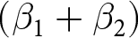 $(\beta_1+\beta_2)$ indicates that their adjustment concentrates on wages and cultivation practices, with increases of 34 and 11 percentage points respectively. There is little response along contractor, technology, or acreage margins. This pattern is consistent with limited short-run adjustment margins in wine production, with responses concentrated in a small set of margins.
The composition of adjustment differs in Napa and Sonoma. The total effect  $(\beta_1+\beta_2+\beta_3)$ shows wage responses of 20 percentage points—smaller than for wine growers elsewhere—alongside larger increases in FLC use (10 percentage points) and cultivation practice changes (22 percentage points).Footnote 3 Notably, wine growers in these counties are significantly less likely to reduce cultivated acreage, consistent with the high establishment costs and long investment horizons that make vineyard conversion costly. The overall pattern suggests that producers in these high-value regions smooth labor demand through organized contracting and adjustments to production practices rather than wages or scale, reflecting both tighter specialized labor markets and limited scope for capital substitution.
Across all groups, adjustment occurs primarily along intensive margins—wages and production practices—with little contemporaneous adoption of labor-saving technology or H-2A participation. The results suggest that short-run responses to labor scarcity in wine grape production are more constrained than in California agriculture broadly.
5.2. 2025–2026 survey
Table 4 reports estimated associations between enforcement-induced labor loss and adaptation strategies from the 2025–2026 survey. Two limitations of this analysis are worth noting. First, the cross-sectional sample is smaller than the 2019 panel, reducing statistical power. These findings should also be interpreted in light of the relatively small wine grape subsample in the 2025–2026 survey, particularly the limited number of growers reporting enforcement-induced labor loss. Although the estimated increase in the probability of adopting at least one adaptation strategy is large and precisely estimated, the small sample size reduces the precision of the individual adaptation margins. Accordingly, the results are best interpreted as evidence that enforcement-induced labor loss prompted a broad behavioral response among affected wine growers, rather than as precise estimates of the magnitude of adjustment through any single channel. Second, identification relies on cross-sectional variation across farmers within counties and commodities. As a result, some coefficients are economically large but imprecisely estimated. For example, the association between labor loss and offering new incentives for wine growers outside of Napa and Somoma is 23 percentage points but not statistically distinguishable from zero.
Enforcement-induced labor loss and adaptation strategies (2025–2026 survey)

Table 4 Long description
Regression coefficients are reported for binary outcomes across six columns: Any strategies, Offered new incentives, Used FLC, Maintained output with fewer workers, Reduced production, and Used H-2A. For Shortage, coefficients are 0.391 with standard error 0.098 for Any strategies, 0.051 with 0.034 for Offered new incentives, 0.093 with 0.056 for Used FLC, 0.060 with 0.058 for Maintained output with fewer workers, 0.101 with 0.056 for Reduced production, and 0.086 with 0.042 for Used H-2A. For Shortage times Wine, coefficients are 0.405 with 0.162, 0.183 with 0.167, 0.201 with 0.212, negative 0.078 with 0.064, 0.257 with 0.213, and negative 0.157 with 0.087, in the same column order. For Shortage times Wine times Napa or Sonoma, coefficients are negative 0.494 with 0.224, negative 0.154 with 0.177, negative 0.200 with 0.212, 0.055 with 0.159, negative 0.265 with 0.221, and 0.069 with 0.061. Total effect for Wine growers outside Napa or Sonoma is 0.797 with 0.119 for Any strategies, 0.233 with 0.157 for Offered new incentives, 0.295 with 0.198 for Used FLC, negative 0.017 with 0.028 for Maintained output with fewer workers, 0.357 with 0.209 for Reduced production, and negative 0.071 with 0.060 for Used H-2A. Total effect for Wine growers in Napa or Sonoma is 0.302 with 0.194, 0.079 with 0.091, 0.095 with 0.078, 0.037 with 0.161, 0.093 with 0.074, and negative 0.002 with 0.028, in the same column order. Observations are 482 in every column, and some coefficients include star markers next to the estimates.
Notes: This table reports estimated associations between enforcement-induced labor loss and adaptation strategies for California farmers in the 2025–2026 survey. All variables are binary indicators equal to one if the farmer reported the given outcome and zero otherwise. A small number of observations are missing because some respondents did not answer all questions. Responses of “Do not know” or otherwise invalid answers are treated as missing. Robust standard errors are in parentheses and clustered at the county level.
*  $p \lt 0.10$, **
 $p \lt 0.05$, ***
 $p \lt 0.01$.
Despite this imprecision in individual estimates, the aggregate response is large and precisely estimated. Non-wine farmers who experienced labor loss are 39 percentage points more likely to adopt at least one adaptation strategy (column 1), while the corresponding effect for wine growers outside of Napa and Sonoma is nearly twice as large at 80 percentage points. These results indicate that enforcement-induced labor loss triggers substantial behavioral responses, even if the specific channels of adjustment are less precisely estimated.
For non-wine farmers, labor loss is associated with production reduction (10 percentage points), although it is only marginally significant. A notable departure from the 2014–2018 period is a positive and statistically significant relationship with H-2A participation (9 percentage points), consistent with the growth in H-2A use over the past decade (Castillo et al., Reference Castillo, Martin and Rutledge2024).
Wine growers outside of Napa and Sonoma show a different pattern. The total effect  $(\beta_1+\beta_2)$ indicates that labor loss increases the likelihood of reducing production by 36 percentage points, the only statistically significant response. This points to fewer short-run adjustment options under enforcement-induced labor loss than under gradual labor market tightening.Footnote 4 Unlike in the earlier period, there is no detectable adjustment through contracting, cultivation practices, or technology adoption, although estimates are imprecise. For wine growers in Napa and Sonoma, no individual strategy is statistically distinguishable from zero, and the overall effect on strategy adoption is likewise imprecisely estimated.
Overall, the 2025–2026 results indicate that enforcement-induced labor loss is associated with a more limited set of responses than the gradual shortages observed over 2014–2018. Adjustment occurs primarily through production reduction rather than input substitution and appears more restricted for wine growers in high-value regions, where reducing output may be more costly in terms of quality or reputation.
5.3. Mechanisms
Having documented that responses differ for wine growers and across regions, we next ask whether these differences reflect labor intensity common to many specialty crops or features specific to wine production.
Table 5 compares responses of wine growers to other labor-intensive crop producers. In the 2014–2018 period, wine growers outside Napa and Sonoma respond similarly to other labor-intensive producers along most margins. The main exception is acreage adjustment: wine growers outside of Napa and Sonoma are 14 percentage points less likely to reduce cultivated acreage, consistent with the greater costs of extensive margin adjustment in perennial viticulture.
Mechanism: Wine versus other labor-intensive crops (2019 survey)

Table 5 Long description
Coefficients compare wine grape growers with other labor intensive crop farmers across seven binary outcomes: any strategies, increased wages, used FLC, adopted labor saving technology, changed cultivation practices, decreased cultivated acres, and used H 2A. For wine outside of Napa and Sonoma, coefficients are minus 0.083 for any strategies, 0.041 for increased wages, minus 0.024 for used FLC, 0.002 for adopted labor saving technology, 0.017 for changed cultivation practices, minus 0.141 with three stars for decreased cultivated acres, and minus 0.002 for used H 2A. For Napa and Sonoma wine compared with other labor intensive crops, coefficients are minus 0.042 for any strategies, minus 0.099 for increased wages, 0.077 with one star for used FLC, minus 0.107 with three stars for adopted labor saving technology, 0.122 with three stars for changed cultivation practices, minus 0.167 with three stars for decreased cultivated acres, and 0.036 with one star for used H 2A. Robust standard errors are shown in parentheses for each coefficient. Observations by column are 2,555, 3,345, 3,265, 3,000, 3,095, 3,315, and 3,305.
Notes: This table reports the results of the statistical tests that compare differences between other labor-intensive crop farmers and wine grape growers for the 2019 survey. All variables are binary indicators equal to one if the farmer reported the given outcome and zero otherwise. A small number of observations are missing because some respondents did not answer all questions. Responses of “Do not know” or otherwise invalid answers are treated as missing. Robust standard errors are in parentheses and clustered at the county level.
*  $p \lt 0.10$, **
 $p \lt 0.05$, ***
 $p \lt 0.01$
Differences are more pronounced for Napa and Sonoma wine growers. Relative to other labor-intensive producers, they are more likely to use FLCs (8 percentage points) and to adjust cultivation practices (12 percentage points), and less likely to adopt labor-saving technology (11 percentage points) or reduce acreage (17 percentage points). Responses in high-value wine regions therefore differ not only from less labor-intensive crops but also from other labor-intensive production systems.
These patterns are consistent with structural features of wine production that distinguish it from other specialty crops. Vineyard acreage is a long-lived, location-specific investment, making extensive margin adjustment more costly than for most hand-harvested crops. Production is also highly quality-sensitive: pruning, canopy management, and harvest require timing and skill that limit substitution toward mechanization or less specialized labor. Wine growers consequently rely on within-season adjustments to production practices and, in high-value regions, on organized labor through contractors, rather than reducing acreage or adopting technology.
Table 6 reports analogous estimates for the 2025–2026 survey. The power concerns noted earlier apply with particular force here, as the smaller cross-sectional sample is further partitioned by crop type and region. Several coefficients are large in magnitude—FLC use and production reduction for wine growers outside of Napa and Sonoma both exceed 25 percentage points—but none are statistically distinguishable from zero except for adoption of at least one strategy. In contrast, the aggregate response is large and precisely estimated. Wine farmers in regions outside Napa and Sonoma who experienced labor loss are 54 percentage points more likely to adopt at least one adaptation strategy compared to other labor-intensive farmers (column 1). However, these effects, as well as those for other strategies, are imprecisely estimated for wine farmers in Napa or Sonoma. The mechanism analysis for the enforcement period is therefore inconclusive, and these estimates should be interpreted accordingly.
Enforcement-induced labor loss and adaptation strategies (2025–2026 survey)

Table 6 Long description
Binary outcomes compare wine grape growers with other labor-intensive crop farmers across six measures: any strategies, offered new incentives, used FLC, maintained output with fewer workers, reduced production, and used H-2A. For wine outside of Napa and Sonoma versus other labor-intensive, coefficients are 0.538 with three asterisks for any strategies, 0.155 for offered new incentives, and 0.267 for used FLC; standard errors are 0.178, 0.185, and 0.213. For Napa and Sonoma wine versus other labor-intensive, coefficients are 0.045 for any strategies, 0.000 for offered new incentives, and 0.068 for used FLC; standard errors are 0.230, 0.115, and 0.100. For wine outside of Napa and Sonoma versus other labor-intensive, coefficients are 0.010 for maintained output with fewer workers, 0.282 for reduced production, and minus 0.176 with one asterisk for used H-2A; standard errors are 0.050, 0.222, and 0.093. For Napa and Sonoma wine versus other labor-intensive, coefficients are 0.066 for maintained output with fewer workers, 0.018 for reduced production, and minus 0.107 for used H-2A; standard errors are 0.167, 0.098, and 0.073. Observations are 482 in each of the six columns. Asterisks appear next to some coefficients to mark statistical significance, and standard errors are shown in parentheses.
Notes: This table reports the results of the statistical tests that compare differences between other labor-intensive crop farmers and wine grape growers for the 2025–2026 survey. All variables are binary indicators equal to one if the farmer reported the given outcome and zero otherwise. A small number of observations are missing because some respondents did not answer all questions. Responses of “Do not know” or otherwise invalid answers are treated as missing. Robust standard errors are in parentheses and clustered at the county level.
*  $p \lt 0.10$, **
 $p \lt 0.05$, ***
 $p \lt 0.01$.
6. Conclusion
Wine producers depend on skilled manual labor for a sequence of time-sensitive operations—pruning, canopy management, thinning, and harvest—that must be completed within narrow windows and cannot readily be performed by machines or less experienced crews, particularly on the hillside terrain characteristic of premium regions. This dependence limits their ability to adjust along many of the margins available to other agricultural producers and makes labor availability a central determinant of production outcomes.
This paper provides evidence on how these constraints bind in California. Using two surveys conducted under distinct labor market conditions, we find that responses to gradual labor market tightening concentrate on wages and cultivation practices, with little recourse to technology adoption, acreage reduction, or the H-2A program. In high-value regions, adjustment shifts toward organized contracting and more intensive cultivation changes. Enforcement-induced labor loss elicits a still narrower set of responses, with production reduction the dominant margin and little evidence of input substitution. Mechanism tests indicate that wine growers respond differently from other labor-intensive crops, implying that labor intensity alone does not account for the observed patterns. The additional constraint reflects structural features of wine production—high-value output, long-lived vineyard capital, quality-sensitive operations, and terrain constraints on mechanization—that limit the scope for adjustment.
These findings bear on a sector already under considerable stress. Demand has softened, demographic turnover raises questions about long-run consumption trends, and production risk from wildfires and smoke taint has increased. Some growers have already begun removing vineyards. Labor constraints compound these pressures in ways that are difficult to offset in the short run, particularly for producers in premium regions where manual labor is most central to product quality. To the extent that enforcement-induced disruptions persist or intensify, the consequences for California wine production may extend well beyond a single season.
Acknowledgments
The authors would like to thank the editor and the anonymous reviewer for their thoughtful and constructive comments, which significantly improved the manuscript. We are especially grateful for the reviewer’s careful engagement with the paper and insightful suggestions regarding the framing, empirical analysis, and interpretation of the results. The authors are also grateful for support from the US Department of Agriculture’s Office of the Chief Economist (award numbers 58-0111-23-002 [Responding to Rising US Farm Labor Costs] and 58-0111-25-017 [Immigration Enforcement and Farm Labor]). The views expressed are those of the authors and do not necessarily represent the views or policy of the US Department of Agriculture or the US government.


 Open access

