



1 Introduction
Curve evolution problems serve as a framework for simulating a variety of phenomena [Reference Cao8], such as crystal growth, phase interface dynamics, and flame propagation. For an embedded curve
 $\gamma $
, its evolution problem can be expressed by
 $$ \begin{align} \frac{\partial \gamma}{\partial t}=\beta N, \end{align} $$
where N is the unit inward normal vector of
 $\gamma $
, and
 $\beta $
is some geometric quantity related to
 $\gamma $
.
By [Reference Gage15, Equation (1.3) and Equation (1.4)] or [Reference Chou and Zhu12, Equation (1.18) and Equation (1.19)], the evolution equations for the length and enclosed area of the evolving curve
 $\gamma $
are given by
 $$ \begin{align} \frac{dl}{dt}&=-\int_\gamma \beta \kappa ds, \end{align} $$
 $$ \begin{align}\hspace{-8pt} \frac{dA}{dt}&=-\int_\gamma \beta ds, \end{align} $$
where s is the arclength parameter. The most famous model in (1.1) is the curve shortening flow for
 $\beta =\kappa $
. According to (1.2) and (1.3), this flow acts as a gradient flow for the length of the evolving curve, and both the length and enclosed area of the curve are non-increasing. It was systematically studied by Gage and Hamilton [Reference Gage and Hamilton17] and Grayson [Reference Grayson23], and the well-known Gage–Hamilton–Grayson theorem (cf. [Reference Andrews, Chow, Guenther and Langford2, Reference Chou and Zhu12]) states that any embedded plane curve evolves into a convex curve and eventually shrinks to a round point under the curve shortening flow.
Professor S. T. Yau proposed an interesting problem concerning curve evolution, specifically whether one can find a parabolic curvature flow that evolves a curve into another one in finite time or infinite time. To research this problem, Lin and Tsai [Reference Lin and Tsai42] introduced an impressive length-preserving flow, which states that a convex curve (i.e., a closed, embedded, and smooth curve with positive curvature everywhere) can be deformed into another curve if the two curves have the same length and the curvature of the evolving curve has a uniform upper bound. Inspired by the “Curvature Difference Flow” suggested by Yau, Gao, and Zhang [Reference Gao and Zhang22] utilized an area-preserving flow, which is a revised version of the “Curvature Difference Flow,” and it evolves a convex curve into another one without extra conditions. For the centro-affine case, Ivaki [Reference Ivaki34] showed a centro-affine curvature flow that deforms a convex curve into an ellipse. In higher dimensions, Stancu [Reference Stancu55] studied a similar question of evolving a smooth closed convex hypersurface into another hypersurface with the same centro-affine curvature. Further recent developments addressing Yau’s problem are available in [Reference Gao20, Reference Liu, Yang and Zhang43].
Another notable category in curve evolution problems is anisotropic curvature flow, which concerns the planar
 $L_p$
Minkowski problem; some work on this topic can be found in [Reference Gage and Li18, Reference Ivaki33, Reference Stancu54, Reference Stancu and Vikram56, Reference Yang, Liu and Fang67], among others. For insightful discussions on the
 $L_p$
Minkowski problem [Reference Lutwak44] and its generalizations from the perspective of curvature flows, it is highly recommended to refer to [Reference Bryan, Ivaki and Scheuer7, Reference Chen, Huang and Zhao9, Reference Chen and Li10, Reference Ding and Li13, Reference Guang, Li and Wang27, Reference Li, Sheng and Wang39, Reference Li, Sheng, Ye and Yi40], and the literature therein. The logarithmic Minkowski problem [Reference Böröczky, Lutwak, Yang and Zhang5] (
 $p = 0$
) is a significant one which is related to the cone-volume measure. For an n-dimensional convex body L, its cone-volume measure is defined by
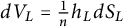 $dV_L=\frac {1}{n}h_L dS_L$
, where
 $h_L$
and
 $dS_L$
are the support function and the surface area measure of L, respectively. The log-Minkowski inequality is pivotal in establishing the uniqueness of the logarithmic Minkowski problem, which remains unsolved. Böröczky et al. [Reference Böröczky, Lutwak, Yang and Zhang4] conjectured that the log-Minkowski inequality
 $$ \begin{align} \int_{S^{n-1}}\log\frac{h_K}{h_L}d\bar{V}_L \geq \frac{1}{n}\log\frac{V(K)}{V(L)} \end{align} $$
holds for two origin symmetric convex bodies K and L, where
 $d\bar {V}_L$
is the cone-volume probability measure of L. They also showed that this is equivalent to the log-Brunn–Minkowski inequality
 $$ \begin{align} V\big(\lambda \cdot K+_{\circ} (1-\lambda) \cdot L\big) \geq V(K)^{\lambda}V(L)^{1-\lambda} \end{align} $$
holds for
 $\lambda \in [0, 1]$
, where the log Minkowski addition
 $\lambda \cdot K+_{o} (1-\lambda ) \cdot L$
is defined as
 $$ \begin{align*} \lambda\cdot K+_{o} (1-\lambda) \cdot L=\bigcap_{u\in S^{n-1}} \left\{x\in \mathbb{R}^n\mid x\cdot u\leq h_K(u)^{\lambda}h_L(u)^{1-\lambda}\right\}. \end{align*} $$
Böröczky et al. [Reference Böröczky, Lutwak, Yang and Zhang4] researched the planar case for (1.4) and (1.5) and showed that the equalities hold in (1.4) and (1.5) if and only if K and L are dilates or K and L are parallelograms with parallel sides. Xi and Leng [Reference Xi and Leng61] introduced the conception of dilation position, and extended the log-Brunn–Minkowski and log-Minkowski inequalities to the nonsymmetric case. They solved Dar’s conjecture in the plane and established the relationship between the log-Brunn–Minkowski inequality and Dar’s conjecture in the plane when convex bodies are at a dilation position. Saroglou [Reference Saroglou52] established the inequality (1.5) with its equality cases for pairs of convex bodies that are both unconditional with respect to some orthonormal basis. Kolesnikov and Livshyts [Reference Kolesnikov and Livshyts35] made significant progress toward the
 $L_p$
Brunn–Minkowski inequality by establishing a local version of this inequality for
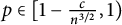 $p\in [1-\frac {c}{n^{3/2}},1)$
, where c is a constant independent of n. They also obtained the local uniqueness of the associated
 $L_p$
Minkowski problem. Chen et al. [Reference Chen, Huang, Li and Liu11] extended the local uniqueness of the
 $L_p$
Minkowski problem in [Reference Kolesnikov and Livshyts35] to the global uniqueness for
 $p\in (p_0,1)$
and
 $p_0<1$
by PDE methods. Recently, a more comprehensive account of various aspects of the
 $L_p$
Brunn–Minkowski and
 $L_p$
Minkowski inequalities can be found in [Reference Böröczky and Kalantzopoulos3, Reference Henk and Pollehn28–Reference Hosle, Kolesnikov and Livshyts30, Reference Kolesnikov and Milman36, Reference Ma, Zeng and Wang45, Reference Milman47, Reference Pan, Yang and Zhu49, Reference Putterman50, Reference Tao, Xiong and Xiong57, Reference Yang, Ye and Zhu64, Reference Yang, Jiang and Zhang66, Reference Yang and Zhang68], and the literature therein.
Before delving into the models of this article, we first introduce the correlation between concepts in convex geometry and anisotropic curvature flows.
Let K be a planar convex body and
 $\gamma $
be its boundary curve with the support function h. If K is smooth, then it can be characterized by the curvature and the support function, with respect to the tangent angle
 $\theta $
of the curve
 $\gamma $
.
Meanwhile, the curvature
 $\kappa $
of
 $\gamma $
can be expressed in terms of its support function h, that is,
 $$ \begin{align} \kappa=\frac{1}{h_{\theta\theta}+h}. \end{align} $$
Let L denote another planar convex body,
 $\tilde {\gamma }$
the boundary curve of L with support function
 $\tilde {h}$
and curvature
 $\tilde {\kappa }$
. The areas of K and L, as well as the mixed area of K with respect to L, are given by (cf. [Reference Green and Osher24])
 $$ \begin{align} V(K)&=\frac{1}{2}\int_0^{2\pi} \frac{h}{\kappa} d\theta=\frac{1}{2}\int_0^{2\pi}\left(h^2-h_\theta^2\right) d\theta, \end{align} $$
 $$ \begin{align} V(L)&=\frac{1}{2}\int_0^{2\pi} \frac{\tilde{h}}{\tilde{\kappa}} d\theta=\frac{1}{2}\int_0^{2\pi}\left(\tilde{h}^2-\tilde{h}_\theta^2\right) d\theta, \end{align} $$
 $$ \begin{align} V(K,L)&=\int_0^{2\pi} \frac{h}{\tilde{\kappa}} d\theta =\int_0^{2\pi} \frac{\tilde{h}}{\kappa} d\theta= \int_0^{2\pi} \left(h\tilde{h}-h_\theta \tilde{h}_\theta \right) d\theta. \end{align} $$
When L is origin symmetric and is an isoperimetrix, we adopt the following notation appearing in Gage’s anisotropic curvature flow [Reference Gage16, p. 454], that is,
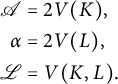 $$ \begin{align*} \mathscr{A}&=2V(K),\\ \alpha&=2V(L),\\ \mathscr{L}&=V(K,L). \end{align*} $$
Clearly,
 $\mathscr {A}$
and
 $\alpha $
represent twice the areas of K and L, respectively, and
 $\mathscr {L}$
is called the Minkowski length of
 $\gamma $
with respect to
 $\tilde {\gamma }$
.
The first aim of this article is to investigate Yau’s problem through the “Curvature Ratio Flow” inspired by Stancu’s centro-affine flow in [Reference Stancu55]. Let
 $\gamma $
and
 $\tilde {\gamma }$
be two origin symmetric planar curves, with
 $\tilde {\gamma }$
being fixed. We consider the following two evolution problems:
 $$ \begin{align} &\frac{\partial \gamma}{\partial t}=\left(\frac{\kappa}{\tilde{\kappa}}-\Lambda_1(t)\right)h N, \end{align} $$
 $$ \begin{align} &\frac{\partial \gamma}{\partial t}=\left(\frac{\kappa}{\tilde{\kappa}}-\Lambda_2(t)\right)\tilde{h} N, \end{align} $$
for
 $\Lambda _1(t)=\frac {\mathscr {L}}{\mathscr {A}}$
and
 $\Lambda _2(t)=\frac {\alpha }{\mathscr {L}}$
, where N is the unit inward normal vector of
 $\gamma $
, and h and
 $\tilde {h}$
are the support functions of
 $\gamma $
and
 $\tilde {\gamma }$
, respectively. From (1.3), we know that both of these flows are area-preserving. The area-preserving flow was first introduced by Gage [Reference Gage15] to better understand the curve shrinking flow, and other recent impressive work on area-preserving flows can be found in [Reference Dittberner14, Reference Gao and Pan19, Reference Gao, Pan and Tsai21, Reference Gao and Zhang22, Reference Wang60], among others.
The main theorem regarding the evolution problem is as follows.
Theorem 1.1 Let
 $\gamma _0$
be an origin symmetric convex curve, and
 $\tilde {\gamma }$
be a fixed origin symmetric convex curve. Then, the flow (1.10a) or (1.10b) exists in
 $[0,\infty )$
. Under this flow, the evolving curve remains symmetric and convex, and keeps its enclosed area. Finally, it converges smoothly to a fixed curve
 $\gamma _\infty $
(congruent to
 $\sqrt {\frac {\mathscr {A}}{\alpha }}\tilde {\gamma }$
) in the
 $C^{\infty }$
sense as time goes to infinity.
The second aim of this article is to investigate some entropy inequalities using area-preserving flows (1.10a) and (1.10b). Entropy plays an important role in both physics and information theory. In physics, entropy is a measure of the degree of disorder in a system, while in information theory, it quantifies the uncertainty of information or the uncertainty of a random variable. Different types of entropy, such as Shannon entropy and relative entropy, establish a direct connection to optimal transportation, Monge–Ampère equations, and geometric inequalities in convex geometry [Reference Villani59].
As applications of the flows (1.10a) and (1.10b), we will show the log-Minkowski inequality and the curvature entropy inequality, which are proven, respectively, in references [Reference Böröczky, Lutwak, Yang and Zhang5, Reference Ma, Zeng and Wang45], under the appropriate entropy associated with the flows. The Brunn–Minkowski inequality can also be obtained from the flows (1.10a) and (1.10b). The “Gauss Curvature Ration” flow, similar to (1.10a), may be a beneficial attempt to address the unsolved log-Minkowski inequality in higher dimensions, which is also a problem that we are considering.
Theorem 1.2 (Log-Minkowski inequality)
Let K and L be two origin symmetric, smooth planar convex bodies. Then,
 $$ \begin{align} \int_{S^1}\log \frac{h_K}{h_L} dV_L \ge \frac{V(L)}{2}\log \frac{V(K)}{V(L)}, \end{align} $$
where the equality holds in (1.11) if and only if K and L are homothetic.
Remark 1.3 From the equivalence of the log-Minkowski inequality (1.4) and the log-Brunn–Minkowski inequality (1.5), we can derive the log-Brunn–Minkowski inequality in the plane. Equality also holds in the inequalities (1.4) and (1.5) when K and L are parallelograms with parallel sides in the discrete case.
Theorem 1.4 (Curvature entropy inequality)
Let K and L be two origin symmetric, smooth planar convex bodies. Then,
 $$ \begin{align} \int_{S^1}\log \frac{\kappa_K}{\kappa_L} dV_L \ge \frac{V(L)}{2}\log \frac{V(L)}{V(K)}, \end{align} $$
where the equality holds in (1.12) if and only if K and L are homothetic.
Remark 1.5 The curvature entropy inequality (1.12) still holds without any symmetry condition but with a dilation position condition for K and L (see [Reference Yang65]). This case can also be proved by flow (1.10b) when
 $\tilde {\gamma }$
is a convex curve with positive support function, the necessary illustration can be found in Remark 2.14 and Remark 3.3, in which the key step is inspired by impressive work in Li and Wang [Reference Li and Wang41].
By the log-Minkowski inequality (1.11) or the curvature entropy inequality (1.12), we can discuss the uniqueness for the cone-volume measure in the smooth setting for origin symmetric planar convex bodies, which is viewed as the uniqueness for the logarithmic Minkowski problem in the smooth setting for origin symmetric planar convex bodies. Specifically, when K and L are origin symmetric, smooth planar convex bodies with same cone-volume measures, then from (1.11), we have
 $$ \begin{align*} \int_{S^1}\log h_K dV_K=\int_{S^1}\log h_K dV_L\ge \int_{S^1}\log h_L dV_L= \int_{S^1}\log h_L dV_K\ge \int_{S^1}\log h_K dV_K, \end{align*} $$
and by (1.12),
 $$ \begin{align*} \int_{S^1}\log \kappa_K dV_K=\int_{S^1}\log \kappa_K dV_L\ge \int_{S^1}\log \kappa_L dV_L= \int_{S^1}\log \kappa_L dV_K\ge \int_{S^1}\log \kappa_K dV_K. \end{align*} $$
From the equality case in (1.11) or (1.12), it yields
 $K=L$
.
Since the speed of flow (1.10a) contains the support function of the evolving curve, it is a locally constrained flow, which has proven to be a powerful tool for exploring geometric inequalities in recent years, especially for Alexandrov–Fenchel inequalities. Notably, recent research has increasingly focused on locally constrained inverse curvature flows, as evidenced by works, such as [Reference Brendle, Guan and Li6, Reference Guan and Li25, Reference Guan and Li26, Reference Hu and Li31, Reference Hu, Li and Wei32, Reference Kwong, Wei, Wheeler and Wheeler38, Reference Mei, Wang and Weng46, Reference Qiang, Weng and Xia51, Reference Scheuer and Xia53, Reference Xia62, Reference Xia63], among others.
The article is structured as follows. In Section 2, we investigate two anisotropic area-preserving flows (1.10a) and (1.10b) for convex curves and establish short-time existence, long-term existence, and convergence. In Section 3, by examining the monotonicity of exact monotonic geometric quantities under flows (1.10a) and (1.10b), we derive some entropy inequalities and the Brunn–Minkowski inequality applicable to convex curves.
2 Anisotropic area-preserving flows
In this section, we first show the short-time existence for flows (1.10a) and (1.10b) by linearization of the evolution equations for the support function of the evolving curve. In order to demonstrate the long-term existence and convergence for flows (1.10a) and (1.10b), we prove that the support function, curvature, and the higher derivatives of both the support function and curvature are uniformly bounded. Finally, we obtain the final shape for flows (1.10a) and (1.10b) through two monotonic geometric quantities.
2.1 Short-time existence
To study the flows (1.10a) and (1.10b), we provide some basic evolution equations based on some basic computations [Reference Chou and Zhu12] or [Reference Gage and Hamilton17].
Lemma 2.1 For flow (1.10a), the evolution equations for the support function h and the curvature
 $\kappa $
are
 $$ \begin{align} h_t&=-\left(\frac{\kappa}{\tilde{\kappa}}-\Lambda_1(t)\right)h, \end{align} $$
 $$ \begin{align} \kappa_t&=\kappa^2\left(\left(\frac{\kappa}{\tilde{\kappa}}h\right)_{\theta\theta}+ \left(\frac{\kappa}{\tilde{\kappa}}h\right)-\frac{\Lambda_1(t)}{\kappa} \right), \end{align} $$
and that for flow (1.10b) are
 $$ \begin{align} &h_t=-\left(\frac{\kappa}{\tilde{\kappa}}-\Lambda_2(t)\right)\tilde{h}, \end{align} $$
 $$ \begin{align} &\kappa_t=\kappa^2\left(\left(\frac{\kappa}{\tilde{\kappa}}\tilde{h}\right)_{\theta\theta}+ \left(\frac{\kappa}{\tilde{\kappa}}\tilde{h}\right)-\frac{\Lambda_2(t)}{\tilde{\kappa}} \right). \end{align} $$
In order to show the short-time existences for the flows (1.10a) and (1.10b), we need to consider the linearization for equations (2.1a) and (2.2a). Actually, we first claim that the support function h is periodic with period
 $2\pi $
. Since the initial curves
 $\gamma _0$
and
 $\tilde {\gamma }$
are convex, they satisfy the closing condition
 $$ \begin{align*} \int_0^{2\pi}\frac{e^{i\theta}}{\kappa_0}d\theta=0\quad \text{and} \quad \int_0^{2\pi}\frac{e^{i\theta}}{\tilde{\kappa}}d\theta=0. \end{align*} $$
Together with the evolution equations of the curvature (2.1b) and (2.2b), one can deduce that
 $$ \begin{align*} \int_0^{2\pi}\frac{e^{i\theta}}{\kappa}d\theta=0, \end{align*} $$
which implies that the evolving curve is periodic with period
 $2\pi $
. Then, by (1.6), we can get that the support function h is also periodic with period
 $2\pi $
.
Next, we deal with the linearization for equations (2.1a) and (2.2a). For (2.1a), by (1.6), (1.7), and (1.9), the functional
 $$ \begin{align} F_1(h)=h_t+\frac{h}{(h_{\theta\theta}+h)\tilde{\kappa}}-\frac{\int_0^{2\pi} \frac{h}{\tilde{\kappa}} d\theta}{\int_0^{2\pi} (h^2-h_{\theta}^2)d\theta}h \end{align} $$
is considered. In fact,
 $F_1$
is an operator from
 $C^{2,\beta }(S^1\times [0,\omega ))$
to
 $C^{\alpha }(S^1\times [0,\omega ))$
for
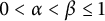 $0<\alpha <\beta \le 1$
. This deduces that the Fréchet derivative of
 $F_1$
at some point
 $h_0>0$
is
 $$ \begin{align*} & DF_1(h_0)[h] \\ &\quad =h_t-\frac{h_0}{((h_0)_{\theta\theta}+h_0)^2\tilde{\kappa}}h_{\theta\theta}+\left(\frac{(h_0)_{\theta\theta}}{((h_0)_{\theta\theta}+h_0)^2\tilde{\kappa}}-\frac{\mathscr{L}(0)}{\mathscr{A}(0)}\right)h\\ &\qquad\! +\frac{h_0}{\mathscr{A}(0)^2} \!\left(2 \mathscr{L}(0)\int_0^{2\pi}h_0h d\theta-2\mathscr{L}(0)\int_0^{2\pi}(h_0)_{\theta}h_{\theta} d\theta-\mathscr{A}(0)\int_0^{2\pi}\frac{h}{\tilde{\kappa}}d\theta \!\right). \end{align*} $$
Thus, the linearization of the evolution equation of the support function h for (2.1a) at
 $h_0$
is
 $$ \begin{align} h_t&=\frac{h_0}{((h_0)_{\theta\theta}+h_0)^2\tilde{\kappa}}h_{\theta\theta}-\left(\frac{(h_0)_{\theta\theta}}{((h_0)_{\theta\theta}+h_0)^2\tilde{\kappa}}-\frac{\mathscr{L}(0)}{\mathscr{A}(0)}\right)h\nonumber\\ &-\frac{h_0}{\mathscr{A}(0)^2}\left(2 \mathscr{L}(0)\int_0^{2\pi}h_0h d\theta-2\mathscr{L}(0)\int_0^{2\pi}(h_0)_{\theta}h_{\theta} d\theta-\mathscr{A}(0)\int_0^{2\pi}\frac{h}{\tilde{\kappa}}d\theta \right).\nonumber\\ \end{align} $$
Similarly, for (2.2a), we consider the functional
 $$ \begin{align*} F_2(h)=h_t+\frac{\tilde{h}}{(h_{\theta\theta}+h)\tilde{\kappa}}-\frac{\int_0^{2\pi} (\tilde{h}^2-\tilde{h}_{\theta}^2)d\theta}{\int_0^{2\pi} \frac{h}{\tilde{\kappa}} d\theta}\tilde{h}. \end{align*} $$
The linearization of the evolution equation of the support function h for (2.2a) at
 $h_0$
is
 $$ \begin{align} h_t&=\frac{\tilde{h}}{((h_0)_{\theta\theta}+h_0)^2\tilde{\kappa}}h_{\theta\theta}+\frac{\tilde{h}}{((h_0)_{\theta\theta}+h_0)^2\tilde{\kappa}}h-\frac{\tilde{h}\alpha}{\mathscr{L}(0)^2}\int_0^{2\pi}\frac{h}{\tilde{\kappa}}d\theta. \end{align} $$
Equations (2.4) and (2.5) are uniformly parabolic with smooth coefficients. It follows from the implicit function theorem of Banach spaces that equations (2.1a) and (2.2a) both have a unique smooth solution over some small time interval (cf. Chou and Zhu [Reference Chou and Zhu12, Section 1.2]). This implies the short-time existence of the flows (1.10a) and (1.10b).


2.2 Long-term existence
Proposition 2.3 The curvature
 $\kappa (\cdot ,t)$
of the evolving curve has a uniform upper bound as long as the flow (1.10a) or (1.10b) exists.
To do this proposition, some necessary lemmas are given.
Lemma 2.4 If an initial curve
 $\gamma _0$
evolves under flow (1.10a) or (1.10b), its Minkowski length
 $\mathscr {L}(t)$
is decreasing.
Proof For flow (1.10a), from (1.7), (1.9), and (2.1a), it has
 $$ \begin{align*} \frac{d \mathscr{L}}{dt}=&\int_0^{2\pi}\frac{h_t}{\tilde{\kappa}}d\theta\\ =&-\int_0^{2\pi}\left(\frac{\kappa}{\tilde{\kappa}}-\Lambda_1(t)\right)\frac{h}{\tilde{\kappa}}d\theta\\ =&-\int_{\tilde{\gamma}}\frac{\kappa h}{\tilde{\kappa}} d\tilde{s} +\frac{\left(\int_{\tilde{\gamma}} h d\tilde{s}\right)^2}{\int_{\tilde{\gamma}} \frac{h\tilde{\kappa}}{\kappa}d\tilde{s}}, \end{align*} $$
where
 $d\tilde {s}=\frac {1}{\tilde {\kappa }}d\theta $
. Due to the Cauchy–Schwarz inequality,
 $\frac {d \mathscr {L}}{dt}\le 0$
and its equality holds if and only if the quantity
 $\frac {\kappa }{\tilde {\kappa }}$
is a positive constant.
Similarly, for flow (1.10b), we have
 $$ \begin{align*} \frac{d \mathscr{L}}{dt}=&\int_0^{2\pi}\frac{h_t}{\tilde{\kappa}}d\theta\\ =&-\int_0^{2\pi}\left(\frac{\kappa}{\tilde{\kappa}}-\Lambda_2(t)\right)\frac{\tilde{h}}{\tilde{\kappa}}d\theta\\ =&-\int_0^{2\pi}\frac{\kappa\tilde{h}}{\tilde{\kappa}^2} d\theta+\frac{\alpha^2}{\mathscr{L}}\\ =&-\int_0^{2\pi}\frac{\kappa\tilde{h}}{\tilde{\kappa}^2} d\theta+\frac{\left(\int_0^{2\pi} \frac{\tilde{h}}{\tilde{\kappa}} d\theta\right)^2}{\int_0^{2\pi}\frac{\tilde{h}}{\kappa} d\theta}. \end{align*} $$
From the Cauchy–Schwarz inequality,
 $\frac {d \mathscr {L}}{dt}\le 0$
with equality holds if and only if the quantity
 $\frac {\kappa }{\tilde {\kappa }}$
is a positive constant.
Lemma 2.5 Suppose that
 $\gamma _0$
is an origin symmetric convex curve. Then, the evolving curve
 $\gamma (\cdot ,t)$
keeps symmetry as long as the flow (1.10a) or (1.10b) exists.
Proof Because
 $\gamma _0$
is an origin symmetric convex curve,
 $\gamma (\cdot +\pi ,0)=\gamma (\cdot ,0)$
. As we know,
 $\gamma (\cdot ,t)$
satisfies (1.10a) (or (1.10b)) with initial
 $\gamma (\cdot ,0)$
, and
 $\gamma (\cdot +\pi ,t)$
satisfies (1.10a) (or (1.10b)) with initial
 $\gamma (\cdot +\pi ,0)$
. Due to Theorem 2.2,
 $\gamma (\cdot +\pi ,t)=\gamma (\cdot ,t)$
as long as the flow (1.10a) (or (1.10b)) exists.
Theorem 2.6 Let
 $\gamma _0$
be an origin symmetric convex curve. If
 $\gamma _0$
evolves according to the flow (1.10a) or (1.10b), then it is always convex.
Proof Suppose that the flow exists in the time interval
 $[0,\omega )$
, and
 $t_0=\inf \{t\mid \kappa (\theta ,t)=0,\theta \in S^1\}<\omega $
. Recall that flows (1.10a) and (1.10b) are area-preserving. Then, by Lemma 2.5, the support function of the evolving curve
 $h(\theta ,t)>0$
for
 $(\theta ,t)\in S^1\times [0,t_0]$
. Otherwise, if the evolving curve had a point where its support function vanishes, the symmetry would imply the existence of nearby points with both positive and negative curvature.
For flow (1.10a), set
 $f_1=\frac {\kappa }{\tilde {\kappa }}he^{\mu _1t}$
, where
 $\mu _1$
is large enough. From (2.1b), it yields that
 $$ \begin{align} (f_1)_t=\left(\frac{\kappa^2}{\tilde{\kappa}}h\right)(f_1)_{\theta\theta}+Q_1(\kappa)f_1, \end{align} $$
where
 $Q_1(\kappa )=\frac {\kappa ^2}{\tilde {\kappa }}h-\frac {\kappa }{\tilde {\kappa }}+\mu _1$
. The quadratic polynomial
 $Q_1(\kappa )$
is positive when
 $\mu _1$
is large enough. Let
 $(f_1)_{\min }(t)=\min \{f(\theta ,t) \mid \theta \in S^1\}$
. We claim that
 $(f_1)_{\min }(t)$
is non-decreasing. If not, there exists an
 $\eta $
, where
 $0 <\eta < (f_1)_{\min }(0)$
, such that at some time
 $t>0$
,
 $(f_1)_{\min }(t)=\eta $
. Set
 $t_1^*=\inf \{t\mid (f_1)_{\min }(t)=\eta \}$
. The continuity of
 $f_1$
ensures that this minimum
 $\eta $
is achieved for the first time at point
 $(\theta _1^*,t_1^*)$
. Then, at this point, we have
 $$ \begin{align*} (f_1)_t\le 0,\quad (f_1)_{\theta\theta}\ge 0, \quad f_1=\eta>0. \end{align*} $$
This contradicts the fact that
 $f_1$
satisfies (2.6), and thus
 $(f_1)_{\min }(t)\ge (f_1)_{\min }(0)$
, which implies that
 $\kappa \ge \frac {\tilde {\kappa }}{h}(f_1)_{\min }(0)e^{-\mu _1t}>0$
for all
 $t\in [0,t_0]$
. It contradicts the hypothesis of
 $t_0$
.
For flow (1.10b), set
 $f_2=\frac {\kappa }{\tilde {\kappa }}\tilde {h} e^{\mu _2t}$
, where
 $\mu _2$
is large enough. By (2.2b), we have
 $$ \begin{align*} (f_2)_t=\left(\frac{\kappa^2}{\tilde{\kappa}}\tilde{h}\right)(f_2)_{\theta\theta}+Q_2(\kappa)f_2, \end{align*} $$
where
 $Q_2(\kappa )=\frac {\kappa ^2}{\tilde {\kappa }}\tilde {h}-\frac {\kappa }{\tilde {\kappa }}\Lambda _2+\mu _2$
. It follows from the Minkowski inequality
 $\mathscr {L}^2\ge \mathscr {A}\alpha $
(see [Reference Gage16]) and Lemma 2.4 that
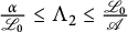 $\frac {\alpha }{\mathscr {L}_0}\le \Lambda _2\le \frac {\mathscr {L}_0}{\mathscr {A}}$
. Hence, the quadratic polynomial
 $Q_2(\kappa )$
is positive when
 $\mu _2$
is large enough. For
 $f_2$
, by a similar discussion as for
 $f_1$
, we can achieve
 $\kappa \ge \frac {\tilde {\kappa }}{\tilde {h}}(f_2)_{\min }(0)e^{-\mu _2t}>0$
for all
 $t\in [0,t_0]$
. This contradicts the hypothesis of
 $t_0$
.
Hence, the evolving curve under flow (1.10a) or (1.10b) is always convex.
To get the upper and lower bounds for support function h, we set
 $$ \begin{align*} h_{\max}(t)=\max_{\theta\in S^1} h(\theta,t)\quad \text{and}\quad h_{\min}(t)=\min_{\theta\in S^1} h(\theta,t). \end{align*} $$
Lemma 2.7 If
 $\gamma (\cdot ,t)$
is an origin symmetric convex solution to flow (1.10a) or (1.10b), then its support function h has uniform upper and lower bounds.
Proof Let
 $\rho (\cdot ,t)$
be the radial function of
 $\gamma (\cdot ,t)$
and
 $\rho _{\max }(t)=\max \limits _{\eta \in S^{1}}\rho (\eta ,t)$
. The radial function
 $\rho (\cdot ,t)$
and the support function
 $h(\cdot ,t)$
have the relation
 $$ \begin{align} \rho(\cdot,t)=\sqrt{h(\cdot,t)^2+h_{\theta}(\cdot,t)^2}. \end{align} $$
If
 $h(\theta ,t)$
reaches its maximum with respect to
 $\theta $
at the point
 $(\theta _1,t)$
, then
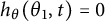 $h_{\theta }(\theta _1,t) = 0$
. It follows from (2.7) that
 $$ \begin{align*} h_{\max}(t)\le \rho_{\max}(t). \end{align*} $$
Similarly,
 $h_{\min }(t)\ge \rho _{\min }(t)$
, where
 $\rho _{\min }(t)=\min \limits _{\eta \in S^{1}}\rho (\eta ,t)$
. If
 $\eta _{\max }\in S^1$
is a value satisfying
 $\rho (\eta _{\max },t)=\rho _{\max }(t)$
, then
 $$ \begin{align*} h(\theta,t)\ge \rho_{\max}(t)|\cos(\theta-\eta_{\max})|, \end{align*} $$
derived from the definition of support function and Lemma 2.5. This together with Lemma 2.4 shows that
 $$ \begin{align*} \mathscr{L}(0)\ge \mathscr{L}(t)&=\int_0^{2\pi} \frac{h(\theta,t)}{\tilde{\kappa}(\theta)} d\theta\ge \rho_{\max}(t)\int_0^{2\pi} \frac{|\cos(\theta-\eta_{\max})|}{\tilde{\kappa}(\theta)}d\theta, \end{align*} $$
which deduces that
 $$ \begin{align} \rho_{\max}(t)\le C_1 =\frac{\mathscr{L}(0)}{\int_0^{2\pi} \frac{|\cos(\theta-\eta_{\max})|}{\tilde{\kappa}(\theta)}d\theta}, \end{align} $$
here
 $C_1$
is a constant independent of t. This yields that
 $$ \begin{align*} h(\theta,t)\le h_{\max}(t)\le \rho_{\max}(t)\le C_1. \end{align*} $$
By the facts that
 $\gamma (\cdot ,t)$
is origin symmetric and
 $\frac {dA}{dt}=0$
, we have
 $$ \begin{align*}\mathscr{A}(0)=\mathscr{A}(t) \le 4\pi \rho_{\min}(t)\rho_{\max}(t)\le 4\pi \rho_{\min}(t)C_1.\end{align*} $$
This tells us
 $$ \begin{align} \rho_{\min}(t)\ge C_2=\frac{\mathscr{A}(0)}{4\pi C_1}. \end{align} $$
Hence,
 $h(\theta ,t)\ge h_{\min }(t)\ge \rho _{\min }(t)\ge C_2$
.
Lemma 2.8 Under flow (1.10a) or (1.10b), the derivation of the support function h for the evolving curve has uniform upper and lower bounds.
Proof From (2.8) and (2.9), we have known that
 $\rho (\cdot ,t)$
has uniform upper and lower bounds. This together with (2.7) yields uniform bounds for
 $h_{\theta }(\cdot ,t)$
.
In order to obtain the upper bound of the curvature
 $\kappa (\cdot ,t)$
, we need to follow Chou’s technique introduced firstly in [Reference Tso58] by discussing the auxiliary quantities. For flow (1.10a), consider
 $$ \begin{align*} \Phi_1(\theta,t)=\frac{ \kappa(\theta,t)h(\theta,t)}{(h(\theta,t)-m_0)\tilde{\kappa}(\theta)} \end{align*} $$
and for flow (1.10b), consider
 $$ \begin{align*} \Phi_2(\theta,t)=\frac{ \kappa(\theta,t)\tilde{h}(\theta)}{(h(\theta,t)-m_0)\tilde{\kappa}(\theta)}, \end{align*} $$
where
 $m_0=\frac {C_2}{2}$
.
Proof of Proposition 2.3
Case 1. For flow (1.10a)
Directly dealing with
 $\Phi _1$
leads to complicated calculations since
 $\Phi _1$
contains
 $\kappa (\cdot ,t)$
and
 $h(\cdot ,\theta )$
. To simplify the calculations and make these computation generality, by (2.7), we have the following equivalent form:
 $$ \begin{align} \Phi_1(\theta,t)=\frac{ \kappa(\theta,t)h(\theta,t)}{(h(\theta,t)-m_0)\tilde{\kappa}(\theta)}=\frac{h(\theta,t)\Lambda_1(t)-h_{t}}{h(\theta,t)-m_0}, \end{align} $$
where
 $m_0=\frac {C_2}{2}$
. Let
 $(\Phi _1)_{\max }(t)=\max \limits _{\theta \in S^1}\Phi _1(\theta ,t)=\Phi _1(\theta _2,t)$
. By Lemma 2.7, the upper bound for
 $\kappa $
is clear when
 $\Phi _1$
achieves its maximum at
 $t=0$
. If
 $\Phi _1(\theta ,t)$
attains its maximum at point
 $(\theta _2,t)$
, where
 $t>0$
, then we have
 $$ \begin{align} (\Phi_1)_\theta=0\quad \text{and}\quad (\Phi_1)_{\theta\theta}\le 0. \end{align} $$
By (2.10), the first and the second derivatives for
 $\Phi _1$
with respect to
 $\theta $
are
 $$ \begin{align*} (\Phi_1)_{\theta}=\frac{h_{\theta}\Lambda_1-h_{t\theta}}{h-m_0}-\frac{(h\Lambda_1 -h_t )h_{\theta}}{(h-m_0)^2} \end{align*} $$
and
 $$ \begin{align*} (\Phi_1)_{\theta \theta}&=\frac{h_{\theta\theta}\Lambda_1-h_{t\theta \theta}}{h-m_0}-\frac{2(h_\theta\Lambda_1 -h_{t\theta})h_{\theta}+(h\Lambda_1 -h_t) h_{\theta\theta}}{(h-m_0)^2}+\frac{2(h\Lambda_1-h_t)h_{\theta}^2}{(h-m_0)^3}\\ &=\frac{h_{\theta\theta}\Lambda_1-h_{t\theta \theta}}{h-m_0}-\frac{2h_\theta}{h-m_0}(\Phi_1)_{\theta}-\frac{(h\Lambda_1 -h_t) h_{\theta\theta}}{(h-m_0)^2}. \end{align*} $$
Combining with (2.11), we can get
 $$ \begin{align} h_{\theta\theta}\Lambda_1-h_{t\theta\theta}\le \frac{h\Lambda_1-h_t}{h-m_0}h_{\theta\theta}=\Phi_1 h_{\theta\theta}. \end{align} $$
By equality (1.6), it yields
 $$ \begin{align*}\kappa_t=-\kappa^2(h_{t}+h_{t\theta\theta}).\end{align*} $$
This together with (2.1a) deduces that
 $$ \begin{align} h_{tt}&=\left(h\Lambda_1-\frac{\kappa h}{\tilde{\kappa}}\right)_t\nonumber\\ &=h_t\Lambda_1+h\frac{d\Lambda_1}{dt}-\frac{1}{\tilde{\kappa}}(\kappa h)_t\nonumber\\ &=h_t\Lambda_1+h\frac{d\Lambda_1}{dt}-\frac{1}{\tilde{\kappa}}( \kappa h_t+\kappa_t h)\nonumber\\ &=h_t\Lambda_1+h\frac{d\Lambda_1}{dt}-\frac{1}{\tilde{\kappa}}(\kappa h_t -\kappa^2(h_t+h_{t\theta\theta})h). \end{align} $$
Then, at point
 $(\theta _2,t)$
, from (2.12) and (2.13), we have
 $$ \begin{align*} (\Phi_1)_t&=\frac{h_t\Lambda_1 +h\frac{d\Lambda_1}{dt}-h_{tt}}{h-m_0}-\frac{(h\Lambda_1-h_t)h_t}{(h-m_0)^2}\\ &=\frac{\kappa h_t}{(h-m_0)\tilde{\kappa}}-\frac{\kappa^2 hh_t}{(h-m_0)\tilde{\kappa}}-\frac{ \kappa^2 h h_{t\theta\theta}}{(h-m_0)\tilde{\kappa}}-\frac{h_t}{h-m_0}\Phi_1\\ &\le \frac{h_t}{h}\Phi_1-h_t\kappa\Phi_1+h_{\theta\theta}\kappa(\Phi_1-\Lambda_1)\Phi_1-\frac{h_t}{h-m_0}\Phi_1\\ &=\frac{h_t}{h}\Phi_1-h_t\kappa\Phi_1+\left(\frac{1}{\kappa}-h\right)\kappa(\Phi_1-\Lambda_1)\Phi_1-\frac{h_t}{h-m_0}\Phi_1\\ &=-\Lambda_1\left(\frac{h}{h-m_0}\right)\Phi_1+\left(1+\frac{m_0}{h}\right)\Phi_1^2-m_0\kappa\Phi_1^2. \end{align*} $$
By (2.10),
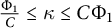 $\frac {\Phi _1}{C}\le \kappa \le C\Phi _1$
holds for a positive constant C. Recall that
 $\Lambda _1(t)=\frac {\mathscr {L}(t)}{\mathscr {A}(t)}\le \frac {\mathscr {L}(0)}{\mathscr {A}(0)}$
. Without loss of generality, assume that
 $\Phi _1\gg 1$
, we finally get the following estimate:
 $$ \begin{align*} (\Phi_1)_t&\le \frac{\mathscr{L}(0)}{\mathscr{A}(0)}\left(\frac{h}{h-m_0}\right)\Phi_1+\left(1+\frac{m_0}{h}\right)\Phi_1^2-m_0\kappa\Phi_1^2\\ &\le \frac{\mathscr{L}(0)}{\mathscr{A}(0)}\left(\frac{h}{h-m_0}\right)\Phi_1^2+\left(1+\frac{ m_0}{h}\right)\Phi_1^2-\frac{m_0}{C}\Phi_1^3\\ &\le C_3 \Phi_1^2-\frac{m_0}{C}\Phi_1^3. \end{align*} $$
This deduces that there exists a positive constant
 $C_4$
independent of t such that
 $\Phi _1(\theta _2,t)\le C_4$
. From Lemma 2.7, we have
 $$ \begin{align*} \kappa(\theta,t)=\frac{\Phi_1(\theta,t)(h(\theta,t)-m_0)\tilde{\kappa}(\theta)}{h(\theta,t)} &\le\frac{\Phi_1(\theta_2,t)(h(\theta,t)-m_0)\tilde{\kappa}(\theta)}{h(\theta,t)} \\ &\le C_4\tilde{\kappa}_{\max}:=C_5, \end{align*} $$
for any point
 $(\theta ,t)$
.
Case 2. For flow (1.10b)
Similarly, due to Lemma 2.7, the upper bound for
 $\kappa $
is achieved when
 $\Phi _2$
attains its maximum at
 $t=0$
. If
 $\Phi _2(\theta ,t)$
attains its maximum at point
 $(\theta _3,t)$
, where
 $t>0$
, then it has
 $$ \begin{align} (\Phi_2)_\theta=0\quad \text{and}\quad (\Phi_2)_{\theta\theta}\le 0. \end{align} $$
Set
 $v=\frac {\kappa }{\tilde {\kappa }}\tilde {h}$
. Due to (2.2b), the evolution equation for v is
 $$ \begin{align} v_t=\frac{\tilde{k}}{\tilde{h}}v^2v_{\theta\theta} +v^2\left(\frac{\tilde{k}}{\tilde{h}}v-\frac{\Lambda_2}{\tilde{h}}\right). \end{align} $$
Then, the first and the second derivatives for
 $\Phi _2$
with respect to
 $\theta $
are
 $$ \begin{align*} (\Phi_2)_{\theta}=\frac{v_{\theta}}{h-m_0}-\frac{v h_{\theta}}{(h-m_0)^2} \end{align*} $$
and
 $$ \begin{align*} (\Phi_2)_{\theta \theta}&=\frac{v_{\theta\theta}}{h-m_0}-\frac{2h_\theta v_\theta}{(h-m_0)^2}+\frac{2h_\theta^2 v}{(h-m_0)^3}-\frac{v h_{\theta\theta}}{(h-m_0)^2}\\ &=\frac{v_{\theta \theta}}{h-m_0}-\frac{2h_\theta}{h-m_0}(\Phi_2)_{\theta}-\frac{v h_{\theta\theta}}{(h-m_0)^2}. \end{align*} $$
Combining with (2.14), it deduces that
 $$ \begin{align} v_{\theta\theta}\le \frac{h_{\theta\theta}}{h-m_0}v. \end{align} $$
Thus, at point
 $(\theta _3,t)$
, we can get
 $$ \begin{align*} 0\le (\Phi_2)_t=&\frac{v_t}{h-m_0}-\frac{v h_t}{(h-m_0)^2}\\ \le&\frac{\tilde{\kappa} h_{\theta\theta}}{(h-m_0)^2\tilde{h}}v^3+\frac{\tilde{\kappa}}{(h-m_0)\tilde{h}}v^3-\frac{\Lambda_2}{(h-m_0)\tilde{h}}v^2-\frac{(\Lambda_2 \tilde{h}-v)v}{(h-m_0)^2}\\ \le &-\frac{\Lambda_2\tilde{h}}{h-m_0}\Phi_2+2\Phi_2^2-\frac{m_0\tilde{k}(h-m_0)}{\tilde{h}}\Phi_2^3, \end{align*} $$
derived from (2.15), (2.16), and (1.6). If
 $\Phi _2\gg 1$
, then
 $$ \begin{align*} 0\le (\Phi_2)_t\le \left(2+\frac{2\Lambda_2\tilde{h}_{\max}}{C_2}-\frac{m_0\tilde{\kappa}(h-m_0)}{\tilde{h}}\Phi_2\right)\Phi_2^2. \end{align*} $$
This implies that
 $$ \begin{align*} \Phi_2\le \left(1+\frac{\Lambda_2\tilde{h}_{\max}}{C_2}\right)\frac{\tilde{h}_{\max}}{m_0\tilde{\kappa}_{\min}C_2}:=C_6. \end{align*} $$
Hence, by Lemma 2.7, we have
 $$ \begin{align*} \kappa(\theta,t)=\frac{\Phi_2(\theta,t)(h(\theta,t)-m_0)\tilde{\kappa}(\theta)}{\tilde{h}(\theta)} &\le\frac{\Phi_2(\theta_2,t)(h(\theta,t)-m_0)\tilde{\kappa}(\theta)}{\tilde{h}(\theta)}\\ &\le \frac{C_6(C_1-m_0)\tilde{\kappa}_{\max}}{\tilde{h}_{\min}}:=C_7, \end{align*} $$
which completes the desired result.
Proposition 2.9 The curvature
 $\kappa (\cdot ,t)$
of the evolving curve has a uniformly lower bound as long as the flow (1.10a) or (1.10b) exists.
Proof Case 1. For flow (1.10a)
Consider the auxiliary function
 $$ \begin{align*} \Psi_1=\log\frac{1}{\kappa}-M_1\log h+\frac{1}{2}\left( h^2+h_{\theta}^2\right), \end{align*} $$
where
 $M_1=\max \limits _{S^1\times (0,T)} (h^2+h_{\theta }^2)+1$
. Assume that
 $\Psi _1$
achieves its maximum at
 $(\theta _0,t_0)$
, then, at this point,
 $$ \begin{align} 0=(\Psi_1)_{\theta}&=\kappa\left(\frac{1}{\kappa}\right)_{\theta}-M_1\frac{h_\theta}{h}+(h h_{\theta}+h_{\theta}h_{\theta\theta})\nonumber\\ &=-\frac{\kappa_\theta}{\kappa}-M_1\frac{h_\theta}{h}+\frac{h_\theta}{\kappa}, \end{align} $$
 $$ \begin{align} 0\ge (\Psi_1)_{\theta\theta}&=-\left(\frac{\kappa_\theta}{\kappa}\right)_{\theta}-M_1\frac{h_{\theta\theta}h-h_{\theta}^2}{h^2}+\frac{h_{\theta\theta}\kappa-h_{\theta}\kappa_{\theta}}{\kappa^2}\nonumber\\ &=-\frac{\kappa_{\theta\theta}\kappa -\kappa_{\theta}^2}{\kappa^2}-M_1\frac{h_{\theta\theta}h-h_{\theta}^2}{h^2}+\frac{h_{\theta\theta}\kappa-h_{\theta}\kappa_{\theta}}{\kappa^2}, \end{align} $$
and
 $$ \begin{align*} 0\le (\Psi_1)_t&=\kappa\left(\frac{1}{\kappa}\right)_{t}-M_1\frac{h_t}{h}+(h h_{t}+h_{\theta}h_{t\theta})\nonumber\\ &=\kappa(h_t +h_{t\theta\theta})-M_1\frac{h_t}{h}+(h h_t+h_\theta h_{t \theta}). \end{align*} $$
Set
 $f=\log \left (\frac {h}{\tilde {\kappa }}\right )$
. From (2.1a), it follows that
 $$ \begin{align*} \log(h\Lambda_1 -h_t )=f+\log \kappa. \end{align*} $$
Differentiating the above equation gives
 $$ \begin{align*} \frac{h_\theta\Lambda_1-h_{t\theta}}{h\Lambda_1 -h_t}=f_\theta+\frac{\kappa_\theta}{\kappa} \end{align*} $$
and
 $$ \begin{align*} \frac{h_{\theta\theta}\Lambda_1-h_{t\theta\theta}}{h\Lambda_1 -h_t}-\frac{(h_\theta\Lambda_1-h_{t\theta})^2}{(h\Lambda_1 -h_t)^2}=f_{\theta\theta}+\frac{\kappa_{\theta\theta}\kappa-\kappa_{\theta}^2}{\kappa^2}. \end{align*} $$
 $$ \begin{align*} \frac{(\Psi_1)_t}{h\Lambda_1 -h_t}&=\kappa\frac{h_t+h_{t\theta\theta}}{h\Lambda_1-h_t}-\frac{M_1}{h}\frac{h_t}{h\Lambda_1-h_t}+\frac{h h_t}{h\Lambda_1-h_t}+\frac{h_{\theta}h_{t\theta}}{h\Lambda_1-h_t}\\ &=\kappa\left(-\frac{h_{\theta\theta}\Lambda_1-h_{t\theta\theta}}{h\Lambda_1-h_t}+\frac{h_{\theta\theta}\Lambda_1+h\Lambda_1-h\Lambda_1+h_t}{h\Lambda_1-h_t} \right)-\frac{M_1}{h}\frac{h\Lambda_1-h\Lambda_1 + h_t}{h\Lambda_1-h_t}\\ &\quad +\frac{h(h\Lambda_1 -h\Lambda_1 + h_t)}{h\Lambda_1-h_t}+\frac{h_{\theta}h_{t\theta}}{h\Lambda_1-h_t}\\ &=\kappa \left( -\frac{(h_\theta\Lambda_1-h_{t\theta})^2}{(h\Lambda_1 -h_t)^2}-\frac{\kappa_{\theta\theta}\kappa-\kappa_{\theta}^2}{\kappa^2}-f_{\theta\theta}\right)\\ &\quad +\frac{(1+h^2-M_1)\Lambda_1}{h\Lambda_1-h_t}-\kappa+\frac{M_1}{h}-h+\frac{h_{\theta}h_{t\theta}}{h\Lambda_1-h_t}\\ & \le \kappa\left( M_1\frac{h_{\theta\theta}h-h_{\theta}^2}{h^2}-\frac{h_{\theta\theta}\kappa-h_{\theta}\kappa_{\theta}}{\kappa^2} -f_{\theta\theta}\right)+\frac{(1+h^2-M_1)\Lambda_1}{h\Lambda_1-h_t}-\kappa \\ &\quad +\frac{M_1}{h}-h+\frac{h_{\theta}h_{t\theta}}{h\Lambda_1-h_t}\\ &=-\kappa M_1\frac{h_\theta^2}{h^2}-\kappa f_{\theta\theta}-h_\theta f_\theta-\frac{1}{\kappa}+\frac{(1+h^2+h_\theta^2-M_1)\Lambda_1}{h\Lambda_1-h_t} \\ &\quad -(1+M_1)\kappa+\frac{2M_1}{h}. \end{align*} $$
By
 $f=\log \left (\frac {h}{\tilde {\kappa }}\right )$
, one has
 $$ \begin{align*} f_{\theta}=-\frac{\tilde{\kappa}_\theta}{\tilde{\kappa}}+\frac{h_\theta}{h} \end{align*} $$
and
 $$ \begin{align*} f_{\theta\theta}=\frac{\tilde{\kappa}_\theta^2-\tilde{\kappa}_{\theta\theta}\tilde{\kappa}}{\tilde{\kappa}^2}+\frac{h_{\theta\theta}h-h_\theta^2}{h^2}=\frac{\tilde{\kappa}_\theta^2-\tilde{\kappa}_{\theta\theta}\tilde{\kappa}}{\tilde{\kappa}^2}-\frac{h_\theta^2}{h^2}+\frac{1}{\kappa h}-1, \end{align*} $$
which together with the smoothness of
 $\tilde {\kappa }$
, Lemmas 2.7 and 2.8 imply that
 $|f_{\theta }|\le C_8$
,
 $|\tilde {\kappa }_{\theta \theta }|\le C_9,$
and
 $$ \begin{align*} -\kappa f_{\theta\theta}&= -\frac{\kappa\tilde{\kappa}_\theta^2}{\tilde{\kappa}^2}+\frac{\tilde{\kappa}_{\theta\theta}\kappa}{\tilde{\kappa}}+\frac{\kappa h_\theta^2}{h^2}-\frac{1}{h}+\kappa\\ &\le \frac{\tilde{\kappa}_{\theta\theta}^2+\kappa^2}{2\tilde{\kappa}}+\frac{\kappa h_\theta^2}{h^2}-\frac{1}{h}+\kappa\\ &\le\frac{C_7^2+C_9^2}{2\tilde{\kappa}_{\max}}+\frac{C_5\tilde{C}_1^2}{C_2^2}+C_5-\frac{1}{h}, \end{align*} $$
where
 $\tilde {C}_1$
is the lower bound for
 $h_\theta $
. Then, we have
 $$ \begin{align*} 0\le \frac{(\Psi_1)_t}{h\Lambda_1 -h_t}&\le \frac{C_7^2+C_9^2}{2\tilde{\kappa}_{\max}}+\frac{h_\theta^2+f_\theta^2}{2}-\frac{C_{10}}{\kappa}+\frac{C_5\tilde{C}_1^2}{C_2^2}+C_5+\frac{2M_1-1}{h}\\ &\le \frac{C_7^2+C_9^2}{2}+\frac{\tilde{C}_1^2+C_8^2}{2}+\frac{2M_1-1}{C_2}+\frac{C_5\tilde{C}_1^2}{C_2^2}+C_5-\frac{C_{10}}{\kappa}, \end{align*} $$
which implies that
 $\kappa (\theta ,t)$
has a positive lower bound independent of t.
Case 2. For flow (1.10b)
For the flow (1.10b), there is the support function associated with a fixed curve denoted by
 $\tilde {\gamma }$
in the evolution equation. However, applying the technique from Case 1 to obtain a lower bound for
 $\kappa $
is challenging. So we need to find another approach to achieve our goal.
Set
 $w=v_\theta $
, then
 $$ \begin{align} w_t&=(v_\theta)_t=(v_t)_\theta\nonumber\\ &=\frac{\tilde{\kappa}}{\tilde{h}}v^2 w_{\theta\theta}+\left( \frac{\tilde{\kappa}}{\tilde{h}}v^2\right)_\theta w_\theta+\frac{\tilde{\kappa}}{\tilde{h}}v^2w+\left( \frac{\tilde{\kappa}}{\tilde{h}}v^2\right)_\theta\left(v-\frac{\Lambda_2}{\tilde{\kappa}}\right)+\frac{\tilde{\kappa}_\theta}{\tilde{\kappa}\tilde{h}}\Lambda_2 v^2. \end{align} $$
We first show the upper bound for w, and consider the quantity
 $$ \begin{align*} \Psi_2=w+\alpha v \end{align*} $$
for
 $\alpha>0$
. The first and second derivatives for
 $\Psi _2$
with respect to
 $\theta $
are
 $$ \begin{align*} (\Psi_2)_\theta&=w_\theta+\alpha w,\\ (\Psi_2)_{\theta\theta}&=w_{\theta\theta}+\alpha w_\theta. \end{align*} $$
Combining with (2.19), we can get
 $$ \begin{align*} (\Psi_2)_t&=w_t+\alpha v_t\\ &=\frac{\tilde{\kappa}}{\tilde{h}}v^2 w_{\theta\theta}+\left( \frac{\tilde{\kappa}}{\tilde{h}}v^2\right)_\theta w_\theta+\frac{\tilde{\kappa}}{\tilde{h}}v^2w+\left( \frac{\tilde{\kappa}}{\tilde{h}}v^2\right)_\theta\left(v-\frac{\Lambda_2}{\tilde{\kappa}}\right)+\frac{\tilde{\kappa}_\theta}{\tilde{\kappa}\tilde{h}}\Lambda_2 v^2\\ &\quad +\alpha\frac{\tilde{\kappa}}{\tilde{h}}v^2\left(w_\theta+v-\frac{\Lambda_2}{\tilde{\kappa}}\right)\\ &=\frac{\tilde{\kappa}}{\tilde{h}}v^2 w_{\theta\theta}+\left[\left( \frac{\tilde{\kappa}}{\tilde{h}}v^2\right)_\theta +\alpha \frac{\tilde{\kappa}}{\tilde{h}}v^2 \right]w_\theta+\frac{\tilde{\kappa}}{\tilde{h}}v^2w \\ &\quad +\left[\left( \frac{\tilde{\kappa}}{\tilde{h}}v^2\right)_\theta +\alpha \frac{\tilde{\kappa}}{\tilde{h}}v^2 \right]\left(v-\frac{\Lambda_2}{\tilde{\kappa}}\right)+\frac{\tilde{\kappa}_\theta}{\tilde{\kappa}\tilde{h}}\Lambda_2 v^2 \\ &=\frac{\tilde{\kappa}}{\tilde{h}}v^2(\Psi_2)_{\theta\theta}+\left( \frac{\tilde{\kappa}}{\tilde{h}}v^2\right)_\theta(\Psi_2)_{\theta}+F(\theta,t) \end{align*} $$
and
 $$ \begin{align*} F(\theta,t)&=\left[\left( \frac{\tilde{\kappa}}{\tilde{h}}\right)_\theta v^2 +\frac{2\tilde{\kappa}}{\tilde{h}}vw\right] (-\alpha w)+\frac{\tilde{\kappa}}{\tilde{h}}v^2w \\ &\quad +\left[\left( \frac{\tilde{\kappa}}{\tilde{h}}\right)_\theta v^2 +\frac{2\tilde{\kappa}}{\tilde{h}}vw+\alpha \frac{\tilde{\kappa}}{\tilde{h}}v^2\right]\left(v-\frac{\Lambda_2}{\tilde{\kappa}}\right)+\frac{\tilde{\kappa}_\theta}{\tilde{\kappa}\tilde{h}}\Lambda_2 v^2\\ &=v\left[- \frac{2\alpha\tilde{\kappa}}{\tilde{h}}w^2+\left( -\alpha \left(\frac{\tilde{\kappa}}{\tilde{h}}\right)_\theta v+\frac{3\tilde{\kappa}}{\tilde{h}} v-\frac{2\Lambda_2}{\tilde{h}} \right)w \right.\\ & \quad \left. +\,\left(\frac{\tilde{\kappa}}{\tilde{h}}\right)_\theta v^2 +\alpha \frac{\tilde{\kappa}}{\tilde{h}}v^2-\frac{\alpha \Lambda_2}{\tilde{h}}v+\frac{\tilde{h}_\theta}{\tilde{h}^2}\Lambda_2 v \right]. \end{align*} $$
Because v and
 $\Lambda _2$
are bounded,
 $F<0$
holds when w is large enough or equivalently
 $\Psi _2$
is large enough. From the maximum principle, we can get the upper bound for
 $\Psi _2$
and thus for w. Similarly, we have the upper bound for
 $-w$
by setting
 $\Psi _2=-w+\alpha v$
with
 $\alpha>0$
. Thus,
 $|w|\le C_{11}$
as long as the flow (1.10b) exists.
Next, we can obtain the lower bound for
 $\kappa $
by the upper bound for w. For any
 $\theta _3,\theta _4\in S^1$
and
 $t>0$
, we have
 $$ \begin{align*} \left|\log\frac{v(\theta_4,t)}{v(\theta_3,t)}\right|=\left|\int_{\theta_3}^{\theta_4} \frac{w(\theta,t)}{v(\theta,t)}d\theta\right|&\le C_{11}\int_{\theta_3}^{\theta_4} \frac{\tilde{\kappa}(\theta)}{\kappa(\theta,t)\tilde{h}(\theta)}d\theta\\ &=C_{11}\int_{\theta_3}^{\theta_4} \frac{\tilde{h}(\theta)}{\kappa(\theta,t)}\ \frac{\tilde{\kappa}(\theta)}{\tilde{h}(\theta)^2}d\theta\\ &\le C_{11}\tilde{C}\mathscr{L}(t)\le C_{12}, \end{align*} $$
where
 $\tilde {C}=\max \{\frac {\tilde {\kappa }(\theta )}{\tilde {h}(\theta )^2}\mid \theta \in S^1\}$
and
 $C_{12}=C_{11}\tilde {C}\mathscr {L}(0)$
. This implies
 $$ \begin{align*} \frac{v_{\max}(t)}{v_{\min}(t)}\le e^{C_{12}}. \end{align*} $$
Notice that
 $$ \begin{align*} \frac{2\pi}{v_{\max}(t)}\le \int_0^{2\pi}\frac{1}{v(\theta,t)}d\theta\le \tilde{C}\mathscr{L}(0). \end{align*} $$
This deduces that
 $$ \begin{align*} v(\theta,t)\ge v_{\min}(t)\ge v_{\max}(t)e^{-C_{12}}\ge \frac{2\pi e^{-C_{12}}}{\tilde{C}\mathscr{L}(0)}. \end{align*} $$
Recall that
 $v=\frac {\kappa }{\tilde {\kappa }}\tilde {h}$
, we can get
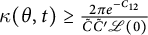 $\kappa (\theta ,t)\ge \frac {2\pi e^{-C_{12}}}{\tilde {C}\tilde {C}'\mathscr {L}(0)}$
, where
 $\tilde {C}'=\max \{\frac {\tilde {h}(\theta )}{\tilde {\kappa }(\theta )}\mid \theta \in S^1\}$
.
Then, we have the long-term existence for the flows (1.10a) and (1.10b).

Proof By Propositions 2.3 and 2.9, we have known that curvature
 $\kappa $
has uniformly positive lower and upper bounds. Since
 $\Lambda _1(t)$
and
 $\Lambda _2(t)$
are bounded, (2.1a) or (2.2a) is uniformly parabolic. From standard regularity theory of uniformly parabolic equations (cf. Krylov [Reference Krylov37]), it yields that
 $$ \begin{align} |h^{(i)}|\le M_i, \end{align} $$
where
 $h^{(i)}$
is the i-th derivative of h, and
 $M_i$
is a positive constant only depending on i and initial curve
 $\gamma _0$
, and the i-th derivative of curvature
 $\kappa $
,
 $\kappa ^{(i)}$
, has uniformly bound, that is,
 $$ \begin{align} |\kappa^{(i)}|\le N_i \end{align} $$
holds for a positive constant
 $N_i$
only depending on i and initial curve
 $\gamma _0$
. This deduces the long-term existence and uniqueness of the smooth solution to the flow (1.10a) or (1.10b).
To obtain the final shape and the convergence of the flow (1.10a) or (1.10b), we need to show the boundedness of
 $\left |\frac {d^2\mathscr {L}}{dt^2}\right |$
.
Lemma 2.11 For the flow (1.10a) or (1.10b), there exists a positive constant
 $C_{13}$
such that
 $$ \begin{align} \left|\frac{d^2\mathscr{L}}{dt^2}\right|\le C_{13}. \end{align} $$
Proof For flow (1.10a), by Lemma 2.4, we have
 $$ \begin{align*} \frac{d^2\mathscr{L}}{dt^2}= -\left(\int_0^{2\pi}\frac{\kappa h}{\tilde{\kappa}^2}d\theta-\Lambda_1(t)\int_0^{2\pi}\frac{h}{\tilde{\kappa}}d\theta\right)_{t}. \end{align*} $$
This together with (2.1b), (1.7), and (2.1a) can yield
 $$ \begin{align*} \frac{d^2\mathscr{L}}{dt^2}&=-\int_0^{2\pi}\frac{\kappa_t h}{\tilde{\kappa}^2}d\theta-\int_0^{2\pi}\frac{\kappa h_t}{\tilde{\kappa}^2}d\theta+\frac{d\Lambda_1(t)}{dt}\int_0^{2\pi}\frac{h}{\tilde{\kappa}}d\theta\\ &=-\int_0^{2\pi} \frac{\kappa^{2}h}{\tilde{\kappa}^2} \left(\frac{\kappa h}{\tilde{\kappa}}\right)_{\theta\theta}d\theta-\int_0^{2\pi} \frac{\kappa^{3}h^2}{\tilde{\kappa}^3} d\theta+\int_0^{2\pi}\frac{\kappa^2 h}{\tilde{\kappa}^3}d\theta+\frac{\mathscr{L}}{\mathscr{A}}\frac{d\mathscr{L}}{dt}\\ &=-\int_0^{2\pi} \frac{\kappa^{2}h}{\tilde{\kappa}^2} \left(\frac{\kappa h}{\tilde{\kappa}}\right)_{\theta\theta}d\theta-\int_0^{2\pi} \frac{\kappa^{3}h^2}{\tilde{\kappa}^3} d\theta \\ &\quad +\int_0^{2\pi}\frac{\kappa^2 h}{\tilde{\kappa}^3}d\theta-\frac{\mathscr{L}}{\mathscr{A}}\int_0^{2\pi}\frac{\kappa h}{\tilde{\kappa}^2}d\theta+\frac{\mathscr{L}^3}{\mathscr{A}^2}. \end{align*} $$
From (2.20) and (2.21), it yields that
 $\left |\frac {d^2\mathscr {L}}{dt^2}\right |$
has a uniform bound.
Similarly, for flow (1.10b), we can get
 $$ \begin{align*} \frac{d^2\mathscr{L}}{dt^2}&= -\left(\int_0^{2\pi}\frac{\kappa\tilde{h}}{\tilde{\kappa}^2}d\theta-\Lambda_2(t)\int_0^{2\pi}\frac{\tilde{h}}{\tilde{\kappa}}d\theta\right)_{t}\\ &=-\int_0^{2\pi}\frac{\kappa_t\tilde{h}}{\tilde{\kappa}^2}d\theta+\frac{d\Lambda_2(t)}{dt}\int_0^{2\pi}\frac{\tilde{h}}{\tilde{\kappa}}d\theta\\ &=-\int_0^{2\pi} \frac{\kappa^{2}\tilde{h}}{\tilde{\kappa}^2} \left(\frac{\kappa\tilde{h}}{\tilde{\kappa}}\right)_{\theta\theta}d\theta-\int_0^{2\pi} \frac{\kappa^{3}\tilde{h}^2}{\tilde{\kappa}^3} d\theta \\ &\quad +\frac{\alpha}{\mathscr{L}}\int_0^{2\pi}\frac{\kappa^2 \tilde{h}}{\tilde{\kappa}^3}d\theta+\frac{\alpha^2}{\mathscr{L}^2}\int_0^{2\pi}\frac{\kappa h}{\tilde{\kappa}^2}d\theta-\frac{\alpha^3}{\mathscr{L}^3}. \end{align*} $$
Proposition 2.12 Under the flow (1.10a) or (1.10b), we have
 $$ \begin{align} \lim_{t\rightarrow \infty}\frac{\kappa(\theta,t)}{\tilde{\kappa}(\theta)}=\sqrt{\frac{\alpha}{\mathscr{A}}}. \end{align} $$
Proof It follows from Theorem 2.10 that the flow (1.10a) or (1.10b) exists on
 $[0,\infty )$
. Let
 $\kappa (\theta ,t_i)$
be a convergent subsequence of the curvature, where
 $t_i\rightarrow \infty $
as
 $i\rightarrow \infty $
. Denote by
 $\kappa _\infty $
the limit of
 $\kappa (\theta ,t_i)$
. Recall that
 $\frac {d\mathscr {L}}{dt}$
is non-positive. We have
 $$ \begin{align*} \int_0^{\infty}\frac{d\mathscr{L}}{dt}dt\ge -\mathscr{L}(0). \end{align*} $$
Then, by (2.11) and Lemma 2.4, it yields that
 $$ \begin{align*} \lim_{t\rightarrow \infty}\frac{d\mathscr{L}}{dt}=0. \end{align*} $$
This deduces that
 $\frac {\kappa }{\tilde {\kappa }}$
is equal to a constant m, and so is
 $\frac {\tilde {h}}{h}$
as time t goes to infinity from the equality case for the Cauchy–Schwarz inequality. In other words,
 $\frac {\kappa _\infty }{\tilde {\kappa }}=m$
and
 $\frac {\tilde {h}}{h_\infty }=m$
. Since
 $$ \begin{align*} \mathscr{A}=\int_0^{2\pi}\frac{h_\infty}{\kappa_\infty}d\theta=\frac{1}{m^2}\int_0^{2\pi}\frac{\tilde{h}_\infty}{\tilde{\kappa}_\infty} d\theta=\frac{\alpha}{m^2}, \end{align*} $$
one has
 $m=\sqrt {\frac {\alpha }{\mathscr {A}}}$
, which is the limit (2.23) for subsequence
 $\{\kappa (\theta ,t_i)\}$
. Since every convergent subsequence of
 $\{\kappa (\cdot ,t)\}$
tends to the same limit, the curvature
 $\kappa $
itself converges.
From (2.20) and (2.21), we have the
 $C^\infty $
convergence of the flow (1.10a) or (1.10b).
Corollary 2.13 For the flow (1.10a) or (1.10b), the convergence of the derivatives
 $$ \begin{align*} \lim_{t\rightarrow \infty} \frac{\partial^i \kappa(\theta,t)}{\partial \theta^i} =\sqrt{\frac{\alpha}{\mathscr{A}}}\frac{\partial^i \tilde{\kappa}(\theta)}{\partial \theta^i} \end{align*} $$
holds for
 $i=1,2,3,\ldots $
.
Proof of Theorem 1.1
Theorem 2.2 asserts the short-time existence of the flow (1.10a) or (1.10b). Lemma 2.5 and Theorems 2.6 and 2.10 demonstrate that any origin symmetric convex curve evolving according to (1.10a) or (1.10b) retains its symmetry, ensuring its long-term existence. Lemma 2.7 and Proposition 2.12 deduce that the evolving curve
 $\gamma (\cdot ,t)$
cannot escape to infinity and converges asymptotically to a fixed curve
 $\gamma _\infty $
which is congruent to
 $\sqrt {\frac {\alpha }{\mathscr {A}}}\tilde {\gamma }$
. Finally, Corollary 2.13 establishes the
 $C^{\infty }$
convergence of flow (1.10a) or (1.10b) as time t approaches infinity.
Remark 2.14 Motivated by the insightful work in Li and Wang [Reference Li and Wang41], the support function of the evolving curve has a uniform bound as long as flow (1.10b) exists, even if the initial curves
 $\gamma _{0}$
and
 $\tilde {\gamma }$
are non-symmetric.
Let
 $\gamma $
be the evolving curve of length l and enclosed area A. The Bonnesen inequality (cf. [Reference Green and Osher24]) states that
 $$ \begin{align} lr-A-\pi r^2\geq 0 \end{align} $$
holds for
 $r_{in}\le r\le r_{out}$
, where
 $r_{in}$
and
 $r_{out}$
are the inradius and outradius of the domain enclosed by
 $\gamma $
, respectively. Then, we have
 $$ \begin{align*} 0<\frac{l-\sqrt{l^2-4\pi A}}{2\pi}\le r_{in}\le r_{out}\le \frac{l+\sqrt{l^2-4\pi A}}{2\pi}. \end{align*} $$
Due to Lemma 2.4, it has
 $$ \begin{align*} l+\sqrt{l^2-4\pi A}\le 2l\le \frac{2}{\tilde{h}_{\min}}\mathscr{L}(t)\le \frac{2}{\tilde{h}_{\min}}\mathscr{L}(0) \end{align*} $$
and
 $$ \begin{align*} \frac{l-\sqrt{l^2-4\pi A}}{2\pi} =\frac{\mathscr{A}(t)}{l+\sqrt{l^2-4\pi A}}\ge \frac{\tilde{h}_{\min}\mathscr{A}(0)}{2\mathscr{L}(0)}. \end{align*} $$
Therefore,
 $2r_0\le r_{in}\le r_{out}\le 2R_0$
, where
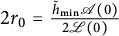 $2r_0=\frac {\tilde {h}_{\min }\mathscr {A}(0)}{2\mathscr {L}(0)}$
and
 $2R_0=\frac {\mathscr {L}(0)}{\pi \tilde {h}_{\min }}$
.
For any fixed time
 $T'\in [0, T)$
, denote by
 $S(T')$
the circle of radius
 $r(T') =2r_0$
inscribed in
 $\gamma (T')$
, with centered
 $P\in R^2$
. For
 $t\ge T'$
, let
 $S(T')$
shrink according to flow
 $\frac {\partial S}{\partial t}=\Lambda \kappa N$
, where
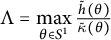 $\Lambda =\max \limits _{\theta \in S^1}\frac {\tilde {h}(\theta )}{\tilde {\kappa }(\theta )}$
. Since each
 $S(t)$
is a circle as long as it exists, the radius of
 $S(t)$
is
 $$ \begin{align*} r(t)=\sqrt{r^{2}(T')-2\Lambda(t-T')}\quad \text{for} \quad t\in \left[T',T'+\frac{r^{2}(T')}{2\Lambda}\right). \end{align*} $$
Comparing the velocity of the flow
 $\frac {\partial S}{\partial t}=\Lambda \kappa N$
with that of the flow (1.10b), it shows that the circle
 $S(t)$
is always enclosed by
 $\gamma (t)$
for all
 $t\in [T',\min \{T'+\frac {r^{2}(T')}{2\Lambda },T\})$
. Hence, the support function of the evolving curve (choose P as the origin) satisfies
 $h(\theta ,t)\ge r(t)$
for
 $(\theta ,t)\in [0,2\pi ]\times [T',\min \{T'+\frac {r^{2}(T')}{2\Lambda },T\})$
. Set
 $\Delta t=\frac {r^{2}(T')}{4\Lambda }$
, we have
 $$ \begin{align*}h(\theta,t)\ge r(t)\ge \sqrt{2}r_0\end{align*} $$
for
 $(\theta ,t)\in [0,2\pi ]\times [T',\min \{T'+\Delta t,T\})$
.
Recalling that the Minkowski length
 $\mathscr {L}(t)$
is decreasing along the flow (1.10b), we obtain the upper bound for the support function, that is,
 $h(\theta ,t)\le \tilde {\kappa }_{\max }\mathscr {L}(t)\le \tilde {\kappa }_{\max }\mathscr {L}(0)$
holds for
 $(\theta ,t)\in [0,2\pi ]\times [T',\min \{T'+\Delta t,T\})$
. The desired result is obtained.
The discussion above is primarily based on Li and Wang [Reference Li and Wang41, pp. 359–361]. To study the gradient flow of an anisoperimetric ratio for convex plane curves without symmetry assumptions, they first established upper and lower bounds for the evolving curve using Bonnesen’s inequality.
Note that the results appearing in Propositions 2.3 and 2.9 are independent of the symmetry. Furthermore, the
 $C^\infty $
convergence for flow (1.10b) is achieved when the initial curves
 $\gamma _0$
and
 $\tilde {\gamma }$
are without symmetry condition. Although an anisotropic model analogous to (1.10b) when
 $\tilde {\gamma }$
is symmetric was discussed in [Reference Pan and Yang48], this work introduces a different method that yields a better convergence result.
3 Entropy inequalities
In this section, we intend to discuss two entropy inequalities, which are the log-Minkowski inequality and the curvature entropy inequality. To do this, we first introduce two monotonic entropy functions under flows (1.10a) and (1.10b).
Lemma 3.1 For the flow (1.10a), the entropy function
 $$ \begin{align*} \mathscr{E}_1(t)=\int_0^{2\pi} \frac{\tilde{h}}{\tilde{\kappa}}\log\frac{h}{\tilde{h}}d\theta \end{align*} $$
is decreasing as time t goes to infinity.
Proof By (2.1a), it has
 $$ \begin{align*} \frac{d\mathscr{E}_1(t)}{dt}&=\int_0^{2\pi} \frac{\tilde{h}}{\tilde{\kappa}}\frac{h_{t}}{h}d\theta\\ &=-\int_0^{2\pi} \frac{\tilde{h}}{\tilde{\kappa}}\left(\frac{\kappa}{\tilde{\kappa}}-\Lambda_1(t)\right)d\theta\\ &=-\int_0^{2\pi}\frac{\kappa\tilde{h}}{\tilde{\kappa}^2}d\theta+\frac{\mathscr{L\alpha}}{\mathscr{A}}. \end{align*} $$
It follows from the Wulff Gage inequality [Reference Green and Osher24, Theorem 0.7] that
 $\frac {d\mathscr {E}_1(t)}{dt}\le 0$
with the equality holds if and only if
 $\gamma $
and
 $\tilde {\gamma }$
are homothetic.
Lemma 3.2 For the flow (1.10b), the entropy function
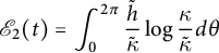 $$ \begin{align*} \mathscr{E}_2(t)=\int_0^{2\pi} \frac{\tilde{h}}{\tilde{\kappa}}\log\frac{\kappa}{\tilde{\kappa}}d\theta \end{align*} $$
is decreasing as time t goes to infinity.
Proof From (2.15) and
 $v=\frac {\kappa }{\tilde {\kappa }}\tilde {h}$
, it yields
 $$ \begin{align*} \frac{d\mathscr{E}_2(t)}{dt}&=\int_0^{2\pi}\frac{\tilde{h}}{\tilde{\kappa}}\frac{v_{t}}{v}d\theta\\ &=\int_0^{2\pi}v\left(v_{\theta\theta}+v-\frac{\Lambda_2(t)}{\tilde{\kappa}}\right)d\theta\\ &=\int_0^{2\pi}v(v_{\theta\theta}+v)d\theta-\frac{\alpha}{\mathscr{L}}\int\frac{\kappa\tilde{h}}{\tilde{\kappa}^2}d\theta. \end{align*} $$
To ensure the monotonicity for
 $\mathscr {E}_2(t)$
, we state an inequality introduced firstly by Andrews in [Reference Andrews1, p. 322, Equation (1.6)], which says that for two curves with corresponding support functions
 $s_1$
and
 $s_2$
,
 $$ \begin{align} \int_0^{2\pi}s_1\tau[s_1]d\theta \int_0^{2\pi}s_2\tau[s_2]d\theta\le \left(\int_0^{2\pi}s_1\tau[s_2]d\theta\right)^2, \end{align} $$
where
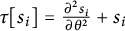 $\tau [s_i]=\frac {\partial ^2 s_i}{\partial \theta ^2}+s_i$
,
 $i=1,2$
. Notice that the above inequality still holds if one of the functions (say
 $s_2$
) has
 $\tau $
strictly positive, and the other is an arbitrary smooth function. Choose
 $s_1=v$
and
 $s_2=h$
, we have
 $$ \begin{align*} \int_0^{2\pi}v(v_{\theta\theta}+v)d\theta \int_0^{2\pi} h(h_{\theta\theta}+h)d\theta \le \left(\int_0^{2\pi} v(h_{\theta\theta}+h)d\theta\right)^2, \end{align*} $$
which together with (1.7) and (1.8) leads to
 $$ \begin{align*} \int_0^{2\pi}v(v_{\theta\theta}+v)d\theta\le \frac{\alpha^2}{\mathscr{A}}. \end{align*} $$
Combining with the Wulff Gage inequality [Reference Green and Osher24, Theorem 0.7], it has
 $$ \begin{align*} \frac{d\mathscr{E}_2(t)}{dt}\le \frac{\alpha^2}{\mathscr{A}}-\frac{\alpha}{\mathscr{L}}\frac{\mathscr{L}\alpha}{\mathscr{A}}=0, \end{align*} $$
which implies the desired result.
The quantity
 $\frac {d\mathscr {E}_2(t)}{dt}$
is equal to
 $0$
if and only if the equalities hold in both the Andrews inequality (3.1) and the Wulff Gage inequality. From [Reference Andrews1, p. 322], we have known that the equality holds in (3.1) only when
 $s_1(z)=ps_2(z)+\langle z,q\rangle $
for some constant p and some point
 $q\in R^2$
. And the equality holds in the Wulff Gage inequality if and only if
 $\gamma $
and
 $\tilde {\gamma }$
are homothetic. Thus,
 $\frac {d\mathscr {E}_2(t)}{dt}=0$
if and only if
 $\gamma $
and
 $\tilde {\gamma }$
are homothetic.
Proof of Theorem 1.2
Denote by K and L the planar convex bodies with boundary
 $\gamma $
and
 $\tilde {\gamma }$
. To obtain the log-Minkowski inequality (1.11), we need only to show the following inequality:
 $$ \begin{align} \int_0^{2\pi} \frac{\tilde{h}}{\tilde{\kappa}}\log\frac{h}{\tilde{h}}d\theta \ge \frac{\alpha}{2}\log\frac{\mathscr{A}}{\alpha}. \end{align} $$
From Lemma 3.1, we have known that
 $\mathscr {E}_1(t)$
is decreasing under flow (1.10a). Since the flow (1.10a) exists in
 $[0,\infty )$
,
 $$ \begin{align*} \int_0^{2\pi} \frac{\tilde{h}}{\tilde{\kappa}}\log\frac{h}{\tilde{h}}d\theta=\mathscr{E}_1(t)\ge \mathscr{E}_1(\infty)=\int_0^{2\pi} \frac{\tilde{h}}{\tilde{\kappa}}\log\frac{h_\infty}{\tilde{h}}d\theta. \end{align*} $$
From the fact that
 $\frac {\tilde {h}}{h_\infty }=\sqrt {\frac {\alpha }{\mathscr {A}}}$
and (1.8), it yields the inequality (3.2). The equality holds in (3.2) if and only if
 $\mathscr {E}_1(t)$
is a constant, which implies that
 $\gamma $
and
 $\tilde {\gamma }$
are homothetic. That is, the equality in the log-Minkowski inequality holds if and only if K and L are homothetic.
Proof of Theorem 1.4
Denote by K and L the planar convex bodies with boundary
 $\gamma $
and
 $\tilde {\gamma }$
. To show the curvature entropy inequality (1.12), we need only to show the following inequality:
 $$ \begin{align} \int_0^{2\pi} \frac{\tilde{h}}{\tilde{\kappa}}\log\frac{\kappa}{\tilde{\kappa}}d\theta \ge \frac{\alpha}{2}\log\frac{\alpha}{\mathscr{A}}. \end{align} $$
Because
 $\mathscr {E}_2(t)$
is decreasing under the flow (1.10b) and this flow exists in
 $[0,\infty )$
, we get
 $$ \begin{align*} \int_0^{2\pi} \frac{\tilde{h}}{\tilde{\kappa}}\log\frac{\kappa}{\tilde{\kappa}}d\theta=\mathscr{E}_2(t)\ge \mathscr{E}_2(\infty)=\int_0^{2\pi} \frac{\tilde{h}}{\tilde{\kappa}}\log\frac{\kappa_\infty}{\tilde{\kappa}}d\theta. \end{align*} $$
Again, by
 $\frac {\kappa _\infty }{\tilde {\kappa }}=\sqrt {\frac {\alpha }{\mathscr {A}}}$
and (1.8), we have the inequality (3.3). The equality holds in (3.3) if and only if
 $\mathscr {E}_2(t)$
is a constant, which implies that
 $\gamma $
and
 $\tilde {\gamma }$
are homothetic. This leads to equality in the curvature entropy inequality if and only if K and L are homothetic.
Remark 3.3 The curvature entropy inequality (1.12) still holds without symmetry condition but with a dilation position condition for two planar convex bodies.
By Remark 2.14, the symmetry requirements for
 $\gamma $
and
 $\tilde {\gamma }$
can be omitted in flow (1.10b). Note that the Wulff Gage inequality holds without symmetry condition but with a dilation position condition for two planar convex bodies (see [Reference Yang65]). Since the entropy
 $\mathcal {E}_2(t)$
is origin-independent and decreases as
 $t \to \infty $
without symmetry requirements, we conclude that inequality (3.3) remains valid without symmetry. Consequently, the curvature entropy inequality (1.12) holds under a dilation position condition.
In conclusion of the article, we also wish to provide the proof of the Brunn–Minkowski inequality in the planar case using flows (1.10a) and (1.10b). In fact, let K and L be the planar convex bodies with boundaries
 $\gamma $
and
 $\tilde {\gamma }$
. Then, by the Steiner formula [Reference Green and Osher24, Proposition 1.4], we have
 $$ \begin{align*}V(K+L)=\frac{1}{2}(\mathscr{A}+2\mathscr{L}+\alpha).\end{align*} $$
Consider the function
 $$ \begin{align*}F(t)=V(K+L)^{\frac{1}{2}}- V(K)^{\frac{1}{2}}-V(L)^{\frac{1}{2}}.\end{align*} $$
It follows from Lemma 2.4 that
 $$ \begin{align*}\frac{dF}{dt}=\frac{1}{2}V(K+L)^{-\frac{1}{2}}\frac{d\mathscr{L}}{dt}\le 0\end{align*} $$
with equality holds if and only if
 $\gamma $
and
 $\tilde {\gamma }$
are homothetic. By Proposition 2.12, it yields that
 $$ \begin{align*}F(t)\ge F(\infty)=(1+m)V(L)^{\frac{1}{2}}-mV(L)^{\frac{1}{2}}-V(L)^{\frac{1}{2}}=0,\end{align*} $$
which implies the Brunn–Minkowski inequality, that is,
 $$ \begin{align*} V(K+L)^{\frac{1}{2}}\ge V(K)^{\frac{1}{2}}+V(L)^{\frac{1}{2}}. \end{align*} $$
Acknowledgements
We are grateful to the anonymous referees for their careful reading of the original manuscript of this article and giving us some invaluable comments.



