1 Introduction
The benchmark case of a boundary layer evolving in a rotating reference frame, commonly called the Ekman layer, represents a simplified model problem to study atmospheric flows, where the interactions between wall-bounded turbulence and stratification can be investigated. For a neutrally stratified Ekman flow at sufficiently high Reynolds number, there is a patterned regime where the turbulence arranges itself into regular streaks or bands obliquely oriented to the direction of mean flow. However, a fully turbulent flow subject to stable stratification can undergo relaminarization and subsequently display a wealth of complex spatio-temporal dynamics. Previous studies have examined spatio-temporal intermittency in canonical turbulent flows (channel, Couette and Ekman layer) finding initial turbulence collapse (Armenio & Sarkar Reference Armenio and Sarkar2002; Flores & Riley Reference Flores and Riley2011), global intermittency where turbulent near-surface patches co-exist with laminar flow (Garcia-Villalba & del Alamo Reference Garcia-Villalba and del Alamo2011; Ansorge & Mellado Reference Ansorge and Mellado2014; Deusebio et al. Reference Deusebio, Brethouwer, Schlatter and Lindborg2014; Deusebio, Caulfield & Taylor Reference Deusebio, Caulfield and Taylor2015), as well as episodes of turbulence collapse followed by recovery to spatially intermittent turbulence (Gohari & Sarkar Reference Gohari and Sarkar2017). Identification of the parameters that distinguish between these different regimes is an important question that is not well understood.
Previous direct numerical simulation (DNS) of the stable Ekman layer have, for the most part, imposed constant-temperature stability wherein the temperature difference,
 $\unicode[STIX]{x0394}\unicode[STIX]{x1D703}_{0}$
, across the boundary layer is fixed (see Ansorge & Mellado Reference Ansorge and Mellado2014; Deusebio et al.
Reference Deusebio, Brethouwer, Schlatter and Lindborg2014; Shah & Bou-Zeid Reference Shah and Bou-Zeid2014). The control parameter based on
 $\unicode[STIX]{x0394}\unicode[STIX]{x1D703}_{0}$
is the bulk Richardson number,
 $Ri_{b}$
defined by (2.9). For sufficiently large
 $Ri_{b}$
, the flow relaminarizes during the initial transient and then recovers in all three aforementioned studies. Ansorge & Mellado (Reference Ansorge and Mellado2014) showed that, after turbulence recovery in their ‘strong stratification’ case with
 $Ri_{b}=0.62$
, the flow has spatial (also called global) intermittency owing to turbulent patches in an otherwise quiescent background. Deusebio et al. (Reference Deusebio, Brethouwer, Schlatter and Lindborg2014) also found co-existing laminar and turbulent regions at
 $Ri_{b}=0.30$
and 0.47. The turbulent component of the heat flux decreased with increasing
 $Ri_{b}$
, but the streamwise fluctuations in the outer layer were larger at
 $Ri_{b}=0.30$
and 0.47, presumably because of the spatial intermittency. Shah & Bou-Zeid (Reference Shah and Bou-Zeid2014) performed a detailed analysis of the budget of second-order statistics and found that it is the reduced shear production of turbulence kinetic energy (TKE,
 $e$
) by buoyancy that is responsible for the decrease of TKE rather than the buoyant destruction of TKE. This feature appears to hold across a variety of stratified shear flows, e.g. uniform shear flow (Jacobitz, Sarkar & VanAtta Reference Jacobitz, Sarkar and Vanatta1997) and channel flow (Armenio & Sarkar Reference Armenio and Sarkar2002), and is related to a decrease in the correlation coefficient between horizontal and vertical fluctuations with increasing values of the gradient Richardson number,
 $Ri_{g}$
.
Recently, Gohari & Sarkar (Reference Gohari and Sarkar2017) performed DNS with a constant buoyancy flux,
 $B_{0}$
, and the Obukhov length scale,
 $L$
defined by (2.5), was changed as the control parameter among cases. They referred to this type of stability as constant-flux stability and found differences with respect to previous cases with constant-temperature stability: the low-level jet is stronger, friction velocity increases with time, there are recurring episodes of collapse and rebirth of turbulence during the transient, and there is a twin-peaked profile of TKE. After a long time of
 $ft=30$
(
 $f$
is the Coriolis frequency), the flow exhibited turbulence with spatial intermittency, there were strong inertial oscillations, and there was no final quasi-steady state. Also, the case with the strongest initial buoyancy flux (
 $L^{-}$
defined in (2.7) was 0.5) ultimately had the largest fluctuation energy because of a stronger low-level jet that became turbulent.
In the nocturnal atmospheric boundary layer (ABL), the stabilizing buoyancy flux is present for a finite time. This motivates the present study of Ekman-layer dynamics where a constant buoyancy flux is applied for a fixed time interval and then the temperature is held constant so that the flow subsequently evolves under a constant
 $Ri_{b}$
. Such a configuration has not been studied previously using DNS, motivating the present work. We focus on the strongly stratified regime wherein turbulence collapses during the initial transient. We are particularly interested in the following questions: What determines the initial collapse and its characteristic time scale? Is there a final quasi-steady state of the flow and, if so, what is this final state? What are the conditions that govern turbulence recovery?
The problem formulation and numerical model are described in § 2. The Obukhov length scale,
 $L^{+}$
, normalized by the viscous scale, has been proposed as a criterion for turbulence collapse (Flores & Riley Reference Flores and Riley2011) and, as elaborated in § 2.2, we choose a fixed value of
 $L^{+}$
and vary the Reynolds number among cases in series A of the simulations. The behaviour of the neutral case at different values of Reynolds number is summarized in § 3. The results of the stratified Ekman layer are discussed in § 4 and an explanation is offered for the qualitative difference in the long-time behaviour that is found at the higher
 $Re$
value of the DNS range. A theoretical analysis is provided in § 5.1 to suggest that the trend with increasing
 $Re$
found here in the DNS holds at higher values of
 $Re$
that are not accessible by DNS. In § 5.2, we examine the influence of the method of stabilization by examining additional simulations (series B) where the
 $Ri_{b}$
achieved at the end of the constant-cooling period in a case of series A is imposed at the start,
 $t=0$
, of the corresponding case of series B. In § 5.3, the effects of different initial values of
 $L^{+}$
at a fixed
 $Re$
is explored (series C). We summarize the results and draw conclusions in § 6.
2 Formulation
The following governing equations, the conservation of momentum under Boussinesq approximation and the advection–diffusion equation for potential temperature, are numerically solved:
 $$\begin{eqnarray}\displaystyle & \displaystyle \frac{\unicode[STIX]{x2202}u_{i}}{\unicode[STIX]{x2202}t}+\frac{\unicode[STIX]{x2202}(u_{i}u_{j})}{\unicode[STIX]{x2202}x_{j}}=-\frac{\unicode[STIX]{x2202}p}{\unicode[STIX]{x2202}x_{i}}+f\unicode[STIX]{x1D716}_{ij3}(u_{j}-U_{\infty }\unicode[STIX]{x1D6FF}_{j1})+\unicode[STIX]{x1D6FF}_{i3}\unicode[STIX]{x1D6FC}g\unicode[STIX]{x1D703}+\unicode[STIX]{x1D708}\unicode[STIX]{x1D6FB}^{2}u_{i}, & \displaystyle\end{eqnarray}$$
 $$\begin{eqnarray}\displaystyle & \displaystyle \frac{\unicode[STIX]{x2202}\unicode[STIX]{x1D703}}{\unicode[STIX]{x2202}t}+\frac{\unicode[STIX]{x2202}(\unicode[STIX]{x1D703}u_{j})}{\unicode[STIX]{x2202}x_{j}}=\unicode[STIX]{x1D706}\unicode[STIX]{x1D6FB}^{2}\unicode[STIX]{x1D703}. & \displaystyle\end{eqnarray}$$
Here,
 $u_{i}$
is the velocity,
 $x_{i}$
is the spatial coordinate,
 $t$
is time,
 $p$
is the pressure deviation from the mean pressure imposed by geostrophic and hydrostatic balance,
 $f$
is the Coriolis parameter,
 $\unicode[STIX]{x1D6FF}_{i3}$
is the Kronecker delta,
 $\unicode[STIX]{x1D716}_{ij3}$
is the Levi-Civita symbol,
 $U_{\infty }$
is the geostrophic wind speed,
 $\unicode[STIX]{x1D6FC}$
is the thermal expansion coefficient of air,
 $g$
is the gravitational acceleration,
 $\unicode[STIX]{x1D708}$
is the molecular viscosity,
 $\unicode[STIX]{x1D703}$
is the deviation of potential temperature from its constant reference value and
 $\unicode[STIX]{x1D706}$
is the thermal diffusivity. The pressure,
 $p$
, is computed by solving the Poisson equation that results from imposing zero velocity divergence at each time step. In the region far above the surface, the Ekman flow is geostrophically balanced, meaning that the Coriolis force exerted on the geostrophic wind balances the large-scale pressure gradient force. Here, the geostrophic wind direction is referred to as streamwise (
 $x$
), the direction of large-scale pressure gradient is referred as spanwise (
 $y$
), and
 $x_{3}=z$
is the vertical direction. No-slip boundary conditions (
 $u_{i}=0$
) are imposed at the bottom surface (
 $x_{3}=z=0$
), and the horizontal boundary conditions are periodic. The top of the domain is taken to be stress free (
 $\unicode[STIX]{x2202}u_{i}/\unicode[STIX]{x2202}x_{3}=0$
) and adiabatic (
 $\unicode[STIX]{x2202}\unicode[STIX]{x1D703}/\unicode[STIX]{x2202}x_{3}=0$
) with a Rayleigh damping layer to minimize the spurious reflection of gravity waves.
The steady-state solution of a neutral Ekman layer is governed by the group
 $\{f,\unicode[STIX]{x1D708},U_{\infty },\unicode[STIX]{x1D706}\}$
. The non-dimensional parameters extracted from this group are the Reynolds number and Prandtl number,
 $$\begin{eqnarray}Re_{D}=\frac{U_{\infty }D}{\unicode[STIX]{x1D708}},\quad Pr=\frac{\unicode[STIX]{x1D708}}{\unicode[STIX]{x1D706}},\end{eqnarray}$$
where
 $D=\sqrt{2\unicode[STIX]{x1D708}/f}$
is the laminar Ekman-layer depth. Since
 $Pr=1$
is fixed in this study, Reynolds number is the only parameter controlling the dynamics of a neutral Ekman flow at steady state. Turbulent Ekman flow is more properly characterized by the surface friction velocity,
 $u_{\ast }$
, and the boundary-layer length scale,
 $u_{\ast }/f$
, leading to the friction Reynolds number,
 $Re_{\ast }$
, as follows
 $$\begin{eqnarray}u_{\ast }^{2}=\unicode[STIX]{x1D708}\frac{\unicode[STIX]{x2202}\sqrt{\langle u\rangle ^{2}+\langle v\rangle ^{2}}}{\unicode[STIX]{x2202}z}\Big|_{x_{3}=0},\quad \unicode[STIX]{x1D6FF}=\frac{u_{\ast }}{f},\quad Re_{\ast }=\frac{u_{\ast }\unicode[STIX]{x1D6FF}}{\unicode[STIX]{x1D708}},\end{eqnarray}$$
where
 $\langle \cdots \rangle$
indicates the spatial average over horizontal planes. It should be mentioned that
 $u_{\ast }$
is not known prior to simulations in an Ekman layer in contrast to channel flow simulations with known pressure gradient, and is observed to be a weak function of
 $Re_{D}$
at sufficiently large Reynolds numbers (Coleman, Ferziger & Spalart Reference Coleman, Ferziger and Spalart1990).
The inner and outer layers of Ekman flow lead to different length scales. The length scale based on wall units,
 $\unicode[STIX]{x1D708}/u_{\ast }$
, is chosen for inner-layer normalization (denoted by superscript
 $+$
) and outer-layer quantities are normalized (denoted by superscript
 $-$
) with the boundary-layer height,
 $\unicode[STIX]{x1D6FF}$
. The friction velocity,
 $u_{\ast _{N}}$
, and boundary-layer height,
 $\unicode[STIX]{x1D6FF}_{N}=u_{\ast _{N}}/f$
, obtained from averages over the last
 $ft=2$
in the neutral case at each given Reynolds number are used for non-dimensionalization. The friction Reynolds number is also computed based on
 $u_{\ast _{N}}$
and
 $\unicode[STIX]{x1D6FF}_{N}$
, unless otherwise noted. Finally, the inverse of the Coriolis parameter,
 $1/f$
, is chosen as the reference time scale.
2.1 Applying finite-time stabilizing buoyancy flux
As discussed in the introduction, previous DNS of the Ekman layer have used either constant-flux stability or constant-temperature stability. The present study incorporates a hybrid boundary condition, i.e. a constant-flux stability for a finite time of
 $fT\approx 6$
and a constant-temperature stability afterwards. In other words, the applied buoyancy flux
 $B_{0}$
is constant over the time interval
 $T$
and the surface cools to a temperature
 $\unicode[STIX]{x1D703}_{0}(T)$
during this interval after which the surface temperature is held constant at
 $\unicode[STIX]{x1D703}_{0}(T)$
. The choice of
 $ft\approx 6$
as the interval of constant buoyancy flux is prompted by the finding of Gohari & Sarkar (Reference Gohari and Sarkar2017) that the initial adjustment of the Ekman layer to the imposed buoyancy flux occurs over approximately an inertial period. At high latitudes with large
 $f$
, night-time cooling can occur over as long as
 $ft\approx 6$
.
Different non-dimensional parameters can be used to characterize the stability imposed on the flow. The Obukhov length,
 $L$
, used to quantify the strength of the buoyancy flux (
 $B_{0}$
is negative for a cooling flux) is defined by
 $$\begin{eqnarray}L=-\frac{u_{\ast }^{3}}{\unicode[STIX]{x1D705}B_{0}},\end{eqnarray}$$
where
 $\unicode[STIX]{x1D705}=0.41$
is the von Kármán constant. Turbulence at a height above
 $L$
is strongly affected by buoyancy. Using inner-layer scaling, the normalized Obukhov length becomes
 $$\begin{eqnarray}L^{+}=\frac{Lu_{\ast }}{\unicode[STIX]{x1D708}}=-\frac{u_{\ast }^{4}}{\unicode[STIX]{x1D705}\unicode[STIX]{x1D708}B_{0}},\end{eqnarray}$$
while outer-layer scaling yields
 $$\begin{eqnarray}L^{-}=\frac{L}{\unicode[STIX]{x1D6FF}_{N}},\end{eqnarray}$$
where
 $\unicode[STIX]{x1D6FF}_{N}=u_{\ast _{N}}/f$
is the scale for the neutral Ekman boundary-layer height. The non-dimensional Obukhov length scale can also be interpreted in terms of the gradient Richardson number at the surface
 $$\begin{eqnarray}Ri_{g,s}=\frac{N^{2}}{S^{2}}=\frac{\unicode[STIX]{x1D6FC}g\unicode[STIX]{x2202}_{x_{3}}\langle \unicode[STIX]{x1D703}_{0}\rangle }{u_{\ast }^{4}/\unicode[STIX]{x1D708}^{2}}=(\unicode[STIX]{x1D705}L^{+})^{-1},\end{eqnarray}$$
where
 $N$
is the buoyancy frequency and
 $S$
is the mean vertical shear (
 $Pr=1$
has been assumed). Therefore,
 $L^{+}$
contains stratification information. Note that, since
 $u_{\ast }$
is a time-dependent function in the stratified DNS cases, so are
 $L$
,
 $L^{-}$
and
 $L^{+}$
.
Bulk Richardson number, a stability measure well suited for constant-temperature stability, is defined as
 $$\begin{eqnarray}Ri_{b}=\unicode[STIX]{x1D6FC}g\unicode[STIX]{x1D6FF}_{N}\frac{\langle \unicode[STIX]{x0394}\unicode[STIX]{x1D703}_{0}\rangle }{U_{\infty }^{2}},\end{eqnarray}$$
where
 $\unicode[STIX]{x0394}\unicode[STIX]{x1D703}_{0}=\unicode[STIX]{x1D703}_{\infty }-\unicode[STIX]{x1D703}_{0}$
is the difference between the temperature above the boundary layer and the surface temperature. In the present study, the surface temperature (
 $\unicode[STIX]{x1D703}_{0}$
) is a time-dependent variable during the time interval,
 $T$
, over which finite-time constant-flux stability is imposed. The value of
 $Ri_{b}$
is also initially dependent on time but it becomes constant at the end of the time interval,
 $T$
.
2.2 Criterion for turbulence collapse
Turbulence in the neutral boundary layer collapses initially if the imposed stability is sufficiently strong. There are several potential candidates for a turbulence-collapse criterion:
 $Ri_{b}$
,
 $L^{-}$
, and
 $L^{+}$
. Previous studies (Ansorge & Mellado Reference Ansorge and Mellado2014; Shah & Bou-Zeid Reference Shah and Bou-Zeid2014) have shown that the critical value of
 $Ri_{b}$
above which neutral Ekman flows undergo initial collapse of turbulence is a function of Reynolds number. Similarly, a
 $Re$
-dependent behaviour is observed for the critical value of
 $L^{-}$
(Flores & Riley Reference Flores and Riley2011; Gohari & Sarkar Reference Gohari and Sarkar2017). These findings are in agreement with previous studies of stratified channel flow at different Reynolds numbers, in which neither
 $(h/L)_{\mathit{cri}}$
(
 $h$
is the half-width of channel) nor
 $Ri_{b}$
was found to be the control parameter of the initial turbulence collapse (Armenio & Sarkar Reference Armenio and Sarkar2002; Nieuwstadt Reference Nieuwstadt2005; Flores & Riley Reference Flores and Riley2011). Cases with the normalized Obukhov length,
 $L^{+}$
, as 650, 705, 683 and 714 exhibited turbulence collapse in the previous studies of Armenio & Sarkar (Reference Armenio and Sarkar2002), Nieuwstadt (Reference Nieuwstadt2005), Flores & Riley (Reference Flores and Riley2011) and Deusebio et al. (Reference Deusebio, Brethouwer, Schlatter and Lindborg2014), respectively. As explained by Flores & Riley (Reference Flores and Riley2011),
 $L^{+}$
is a measure of the dynamic range between the buoyancy constraint of
 $L$
on the large-eddy length and
 $\unicode[STIX]{x1D708}/u_{\ast }$
that represents the small-eddy length scale of the pre-existing near-wall turbulence. If
 $L^{+}$
becomes sufficiently small during the flow evolution (less than 100 according to Flores & Riley (Reference Flores and Riley2011) in a stratified channel), turbulence cannot be maintained in wall-bounded flows since buoyancy influences the entire dynamic range of turbulence scales. It is worth noting that the collapse criterion of
 $L^{+}=100$
was inferred by (Flores & Riley Reference Flores and Riley2011) from a stratified channel with an initial
 $L^{+}=683$
. The field measurements of CASES-99 campaign, a comprehensive collection of flow statistics taken for 28 nights with clear sky conditions (Poulos et al.
Reference Poulos, Blumen, Fritts, Lundquist, Sun, Burns, Nappo, Banta, Newsom, Cuxart and Terradellas2002) provide further guidance. Banta et al. (Reference Banta, Mahrt, Vickers, Sun, Balsley, Pichugina and Williams2007) analysed the typical structure of five very stable nights from the CASES-99 campaign and discussed implications of turbulent exchange between the surface layer and the upper layers of the lower atmosphere. While the studied nights showed a typical
 $L^{+}\approx O(10^{4})$
, the lowest reported value of
 $L^{+}$
with turbulence was 667.
As noted in the introduction, we are interested in studying the stable regime where turbulence initially collapses. According to the above literature review, application of a cooling flux with
 $L_{\mathit{cri}}^{+}\approx 700$
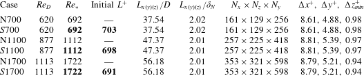
to a neutral boundary layer is hypothesized to be sufficient for turbulence collapse and we conduct series A of the DNS with initial
 $L^{+}\approx 700$
. The degree of Reynolds independence of the
 $L_{\mathit{cri}}^{+}\approx 700$
condition for turbulence collapse is ascertained considering three Reynolds numbers,
 $Re_{\ast }=\{692,1112,1722\}$
. At each Reynolds number, a separate simulation is performed wherein a neutral Ekman boundary layer is allowed to evolve and reach a quasi-steady-state condition for approximately one inertial oscillation. At the beginning of the stratification phase, a constant stabilizing buoyancy flux,
 $B_{0}$
, corresponding to initial
 $L^{+}\approx 700$
is applied at the surface for a finite time of
 $fT\approx 6$
, and the surface temperature is held constant afterwards. We investigate the flow evolution subsequent to the imposed stratification in these three cases.
DNS parameters of simulated cases in series A. The case label in column 1 starts with N (neutral case) or
 $S$
(stable case) and has a number corresponding to the target value of friction Reynolds number,
 $Re_{\ast }$
. In the stable cases, a surface buoyancy flux, chosen to obtain a target
 $L^{+}\approx 700$
, is applied for a finite time of
 $fT\approx 6$
and then the surface temperature is held constant. Note that
 $\unicode[STIX]{x1D6FF}_{N}$
is a measured parameter calculated from averages over the last
 $ft=2$
of the neutrally stratified simulation at each Reynolds number. The numbers in bold signify the controlling parameters in the simulations.

2.3 Numerical model
The numerical model used to solve (2.1) and (2.2) is a modified version of that developed by Jalali, Rapaka & Sarkar (Reference Jalali, Rapaka and Sarkar2014) and Gohari & Sarkar (Reference Gohari and Sarkar2017). Major features of this solver are as follows: (i) a low storage, third-order Runge–Kutta method is used as the time marching algorithm; (ii) derivatives in the spanwise direction are computed using Fourier transforms, while the derivatives in the other two directions are computed using the central second-order finite difference method; and (iii) dealiasing of nonlinear terms is performed using the
 $3/2$
rule.
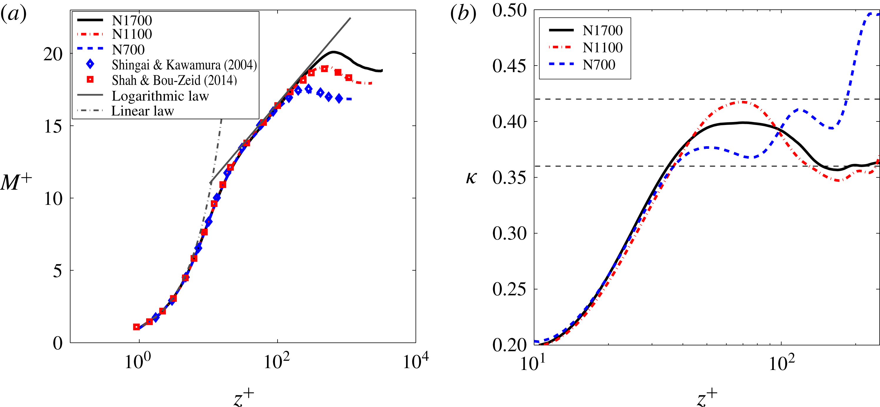
Time-averaged statistics for neutrally stratified cases. (a) Mean velocity profile compared with the numerical studies of Shah & Bou-Zeid (Reference Shah and Bou-Zeid2014) and Shingai & Kawamura (Reference Shingai and Kawamura2004), and the logarithmic law:
 $M^{+}=(1/\unicode[STIX]{x1D705})\ln (z^{+})+B$
, where
 $M=\sqrt{\langle u\rangle ^{2}+\langle v\rangle ^{2}}$
is the mean horizontal velocity magnitude and
 $B=5.3$
is a constant. (b) The von Kármán constant,
 $\unicode[STIX]{x1D705}$
, computed from the neutrally stratified cases (see (3.1)). The typical range of von Kármán constant reported in the literature (0.36–0.41) is shown by the two horizontal dashed lines. The time averaging is performed over the last
 $ft\approx \unicode[STIX]{x03C0}$
.

Table 1 presents a summary of the simulated cases of series A. The stratified-flow simulations have the same initial value of
 $L^{+}\approx 700$
while
 $Re_{\ast }$
is varied among cases. An important requirement in DNS is the proper resolution of viscous effects near the surface which can extend up to
 $z^{+}=10$
. The viscous sublayer has 12 points in the neutral simulation with a non-dimensional vertical grid spacing,
 $\unicode[STIX]{x0394}z_{\mathit{min}}^{+}\leqslant 1$
. The grid is stretched moving upwards, but the grid spacing does not exceed
 $\unicode[STIX]{x0394}z^{+}=18$
at the top of the boundary layer in all cases. The streamwise resolution is
 $\unicode[STIX]{x0394}x^{+}\approx 8.7$
and the spanwise resolution is
 $\unicode[STIX]{x0394}y^{+}\approx 4.9$
similar to the previous DNS studies of wall-bounded turbulent flows (Flores & Riley Reference Flores and Riley2011; Ansorge & Mellado Reference Ansorge and Mellado2014; Gohari & Sarkar Reference Gohari and Sarkar2017). Boundary conditions correspond to no-slip and impermeability at the surface, and stress free and adiabatic at the top. To minimize spurious reflection of internal gravity waves in each case, a Rayleigh damping layer of 10 points is used at the top. In all the simulated cases, the domain size is similar to the one used in the recent studies of Shah & Bou-Zeid (Reference Shah and Bou-Zeid2014) and Gohari & Sarkar (Reference Gohari and Sarkar2017), which is observed to be sufficient to capture all the dynamically active turbulence scales.
3 Neutral Ekman boundary layer
The neutral Ekman boundary layer is simulated for three different values of Reynolds number. Statistics are obtained by horizontal plane averages and further time averaging over an interval of
 $ft\approx 2$
when a quasi-steady state is achieved (after about
 $ft=\unicode[STIX]{x03C0}$
in each case). Figure 1(a) shows the mean velocity profiles at different Reynolds numbers in comparison with the numerical studies of Shingai & Kawamura (Reference Shingai and Kawamura2004) and Shah & Bou-Zeid (Reference Shah and Bou-Zeid2014). The linear law (given by
 $M^{+}=z^{+}$
, where
 $M=\sqrt{\langle u\rangle ^{2}+\langle v\rangle ^{2}}$
is the mean horizontal velocity magnitude) in the viscous sublayer and the logarithmic law (given by
 $M^{+}=(1/\unicode[STIX]{x1D705})\ln (z^{+})+B$
where
 $B=5.3$
is a constant) are also shown. The logarithmic region, shown by a plateau of relatively constant
 $\unicode[STIX]{x1D705}$
in figure 1(b), is present at
 $Re_{\ast }=1700$
but is limited to a narrow region. The von Kármán ‘constant’,
 $\unicode[STIX]{x1D705}(z)$
is computed using
 $$\begin{eqnarray}\frac{\unicode[STIX]{x1D705}z}{u_{\ast }}\bigg[\bigg(\frac{\unicode[STIX]{x2202}\langle u\rangle }{\unicode[STIX]{x2202}z}\bigg)^{2}+\bigg(\frac{\unicode[STIX]{x2202}\langle v\rangle }{\unicode[STIX]{x2202}z}\bigg)^{2}\bigg]^{1/2}=1.\end{eqnarray}$$
Similar to the previous findings of Shah & Bou-Zeid (Reference Shah and Bou-Zeid2014) and Ansorge & Mellado (Reference Ansorge and Mellado2016),
 $\unicode[STIX]{x1D705}(z)$
exhibits a strong decline from
 $\unicode[STIX]{x1D705}(z^{+}\approx 50)\approx 0.41$
to
 $\unicode[STIX]{x1D705}\approx 0.36$
at the upper end of logarithmic layer. A possible reason for this dip can be the existence of external intermittency at this range of heights of Ekman flow (Ansorge & Mellado Reference Ansorge and Mellado2016). Nevertheless, laboratory experiments, atmospheric observations and previous DNS studies have indicated relatively weak variation of
 $\unicode[STIX]{x1D705}$
values inside the logarithmic region of the boundary layer, ranging between 0.36 and 0.42 (Spalart, Coleman & Johnstone Reference Spalart, Coleman and Johnstone2008; Shah & Bou-Zeid Reference Shah and Bou-Zeid2014; Ansorge & Mellado Reference Ansorge and Mellado2016), compared to its significant variation outside. In the present work hereafter, a constant value of
 $\unicode[STIX]{x1D705}=0.41$
is used unless otherwise noted.
The normalized surface friction velocity,
 $u_{\ast }/U_{\infty }$
, and the veering angle of the surface stress with respect to the geostrophic velocity,
 $\unicode[STIX]{x1D6FD}$
, show a weak dependence on
 $Re$
and are as follows:
 $\{u_{\ast }/U_{\infty },\unicode[STIX]{x1D6FD}\}$
takes the value
 $\{0.0589,24.85^{\circ }\}$
in case N700,
 $\{0.05551,21.40^{\circ }\}$
in case N1100 and
 $\{0.0522,19.2^{\circ }\}$
in case N1700. It is worth noting that these values are in good agreement with those predicted by the correlation introduced by Coleman et al. (Reference Coleman, Ferziger and Spalart1990) (
 $\unicode[STIX]{x1D6FD}=45^{\circ }$
in the laminar state).
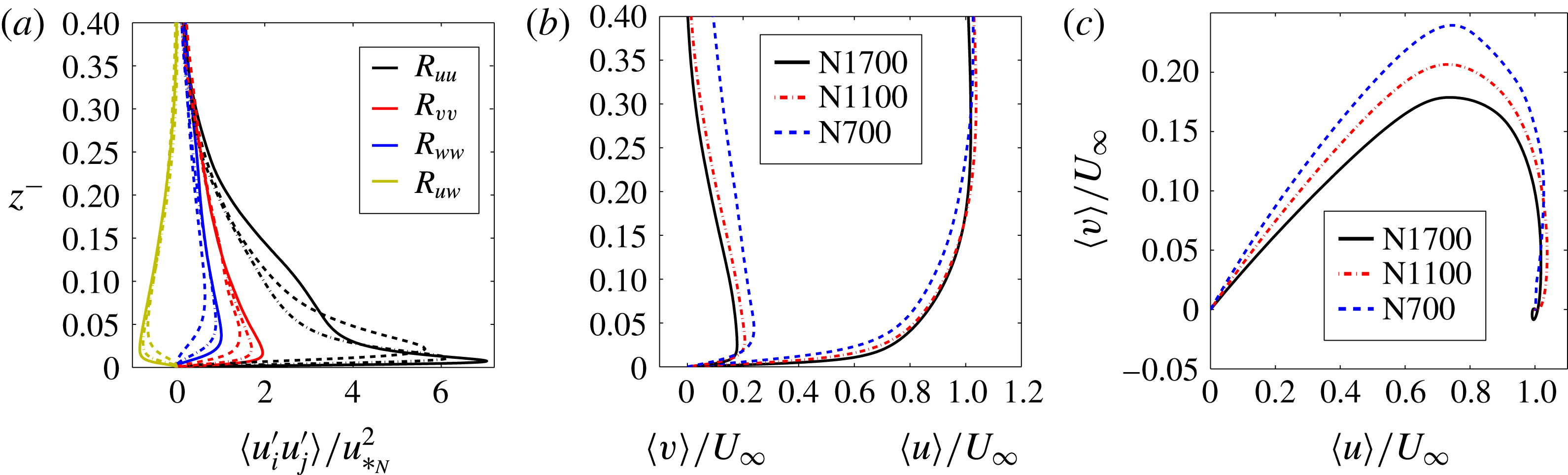
Figure 2(a) compares the Reynolds stresses, plotted using outer-layer scaling at different Reynolds numbers. The near-surface region (
 $z^{-}<0.3$
) contains the most vigorous turbulent activity. Upon increasing the Reynolds number, the absolute peak value of each Reynolds stress increases, while the normalized height at which this maximum occurs decreases. Moreover, the streamwise Reynolds stress shows an enhancement in the outer layer with increasing
 $Re_{\ast }$
, similar to the recent wall-bounded studies at high Reynolds numbers (Hultmark et al.
Reference Hultmark, Vallikivi, Bailey and Smits2012; Bernardini, Pirozzoli & Orlandi Reference Bernardini, Pirozzoli and Orlandi2014; Pirozzoli, Bernardini & Orlandi Reference Pirozzoli, Bernardini and Orlandi2014). The Ekman spiral, shown in figure 2(c), depicts the structure of near-surface wind in which the flow rotates counterclockwise as one moves upward from the surface. It is clear that the surface veering angle decreases when
 $Re_{\ast }$
increases.
Flow statistics for neutrally stratified cases. Profiles of: (a) normalized Reynolds stresses as a function of normalized height (
 $z^{-}=z/\unicode[STIX]{x1D6FF}_{N}$
) (solid, dot-dashed and dashed lines correspond to case N1700, N1100 and N700, respectively); (b) normalized mean velocity profiles; and (c) Ekman spiral (or velocity hodograph). Time averaging of horizontally averaged statistics is performed over last
 $ft\approx 2$
.

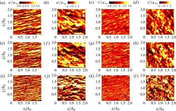
Velocity fluctuations on horizontal planes for neutrally stratified cases, N700 (a–d), N1100 (e–h) and N1700 (i–l): (a,e,i) streamwise velocity fluctuation,
 $u^{\prime }/u_{\ast _{N}}$
, at height
 $z^{+}=15$
, (b,f,j) streamwise velocity fluctuation,
 $u^{\prime }/u_{\ast _{N}}$
, at height
 $z^{-}=0.2$
, (c,g,k) spanwise velocity fluctuation,
 $v^{\prime }/u_{\ast _{N}}$
, at height
 $z^{+}=15$
, (d,h,l) spanwise velocity fluctuation,
 $v^{\prime }/u_{\ast _{N}}$
, at height
 $z^{-}=0.2$
.

Figure 3 shows visualizations of normalized streamwise velocity fluctuation,
 $u^{\prime }/u_{\ast _{N}}$
(columns headed a,b) and spanwise velocity fluctuation,
 $v^{\prime }/u_{\ast _{N}}$
(columns headed c,d), on the horizontal planes near the surface (columns headed a,c at
 $z^{+}=15$
) and on the outer-layer horizontal planes (columns headed b,d at
 $z^{-}=0.2$
) for the neutrally stratified cases. The streamwise velocity fluctuations present inclined streak-like structures near the surface, while the structures at
 $z^{-}=0.2$
are larger. At a larger Reynolds number, the thickness and the angle of these structures (which is close to
 $\unicode[STIX]{x1D6FD}$
) decrease. The spanwise velocity fluctuations near the surface are also organized into structures aligned along the surface veering angle, while the structures at
 $z^{-}=0.2$
are inclined at a different angle.
4 Stably stratified Ekman boundary layer
In series A of the simulations, a neutrally stratified turbulent Ekman layer is exposed to a constant surface buoyancy flux for a finite time interval of
 $ft\approx 6$
. The value of the buoyancy flux corresponds to a nominal initial value of
 $L^{+}\approx 700$
and three values of
 $Re_{\ast }$
are considered (see table 1 and the discussion of § 2.1). The results are discussed in the following subsections.
4.1 Turbulence collapse and transitional Ekman layer
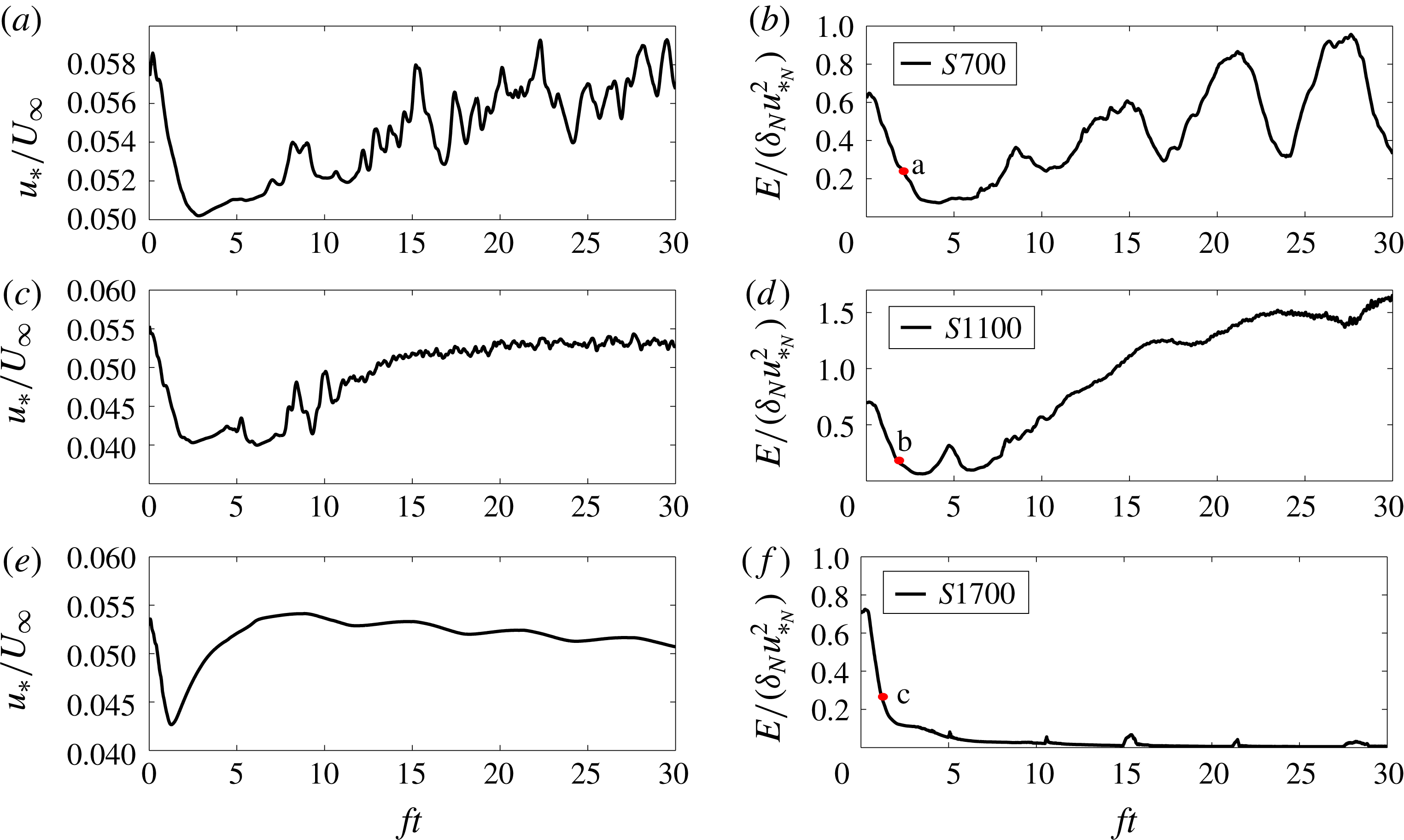
The stabilizing buoyancy flux leads to an initial period of collapsed turbulence, emergence of a low-level jet (LLJ) and the formation of a thermal inversion in all cases. The time evolution of normalized friction velocity in figure 4(a,c,e) shows that all the cases have an initial decrease of surface drag that is followed by an increase. The initial decay rate of
 $u_{\ast }/U_{\infty }$
is larger at higher Reynolds numbers with a typical drop of approximately
 $20\,\%$
in magnitude. Although the normalized friction velocity in the low-
 $Re$
case
 $S700$
follows the general trend of an increase after
 $ft\approx 4$
, its late-time behaviour is quite intermittent and the entire lower flank of the LLJ exhibits oscillations in the shear and the direction. In case
 $S1100$
, the LLJ oscillation near the surface is temporally less intermittent and there is an almost constant
 $u_{\ast }/U_{\infty }$
at a late time. The difference in the late-time behaviour of these cases is elaborated in § 4.2. In case
 $S1700$
with the higher
 $Re_{\ast }$
, the normalized friction velocity increases during the LLJ emergence; however, in contrast to the other cases,
 $u_{\ast }/U_{\infty }$
exhibits a trend of consistent decrease at late time with an oscillatory modulation at the inertial period of
 $ft=2\unicode[STIX]{x03C0}$
.
The time evolution of: (a,c,e) normalized friction velocity (
 $u_{\ast }/U_{\infty }$
); and (b,d,f) integrated turbulent kinetic energy (
 $E/(\unicode[STIX]{x1D6FF}_{N}u_{\ast _{N}}^{2})$
), for stably stratified cases at
 $Re_{\ast }=692$
(a,b),
 $Re_{\ast }=1112$
(c,d) and
 $Re_{\ast }=1722$
(e,f). The finite-time buoyancy flux is imposed on a neutral Ekman layer at
 $ft=0$
for one inertial oscillation (
 $ft\approx 6$
). The letters correspond to the panels of figure 7.

There is a striking influence of Reynolds number on the time evolution of the integrated TKE (figure 4 b,d,f) defined by
 $$\begin{eqnarray}E=\int e\,\text{d}x_{3}=\frac{1}{2}\int _{0}^{L_{z}}\langle u_{i}^{\prime }u_{i}^{\prime }\rangle \,\text{d}x_{3}.\end{eqnarray}$$
In the higher-
 $Re$
case
 $S1700$
shown in figure 4(f), the TKE does not recover at long time while it does in the lower-
 $Re$
simulations. In all cases, the normalized
 $E$
initially decreases to nearly zero during a ‘decay period’, indicating a turbulence collapse within the interval of constant buoyancy flux. This confirms that the choice of
 $L_{\mathit{cri}}^{+}\approx 700$
results in collapsed turbulence during the initial transient, independent of Reynolds number.
The TKE recovery in case
 $S700$
(figure 4
b) is not monotonic and there is noticeable temporal intermittency in the TKE. The period of large-amplitude oscillations of the integrated TKE corresponds to the inertial period,
 $ft=2\unicode[STIX]{x03C0}$
. The oscillations are less pronounced in case
 $S1100$
with an intermediate
 $Re_{\ast }$
.
As noted above, case
 $S1700$
exhibits a decay period with collapsed turbulence, however, unlike case
 $S1100$
, collapse is not followed by a recovery period. This difference between the two cases is due to the stronger bulk stability of case
 $S1700$
that is an indirect effect of the change in
 $Re_{\ast }$
among cases. All cases have a similar initial
 $L^{+}$
but the larger value of
 $Re_{\ast }$
in case
 $S1700$
requires a larger surface buoyancy flux to achieve the same initial
 $L^{+}$
as will be discussed in § 4.3 and, therefore, the value of
 $Ri_{b}(t)$
(see figure 10 and its discussion) in case
 $S1700$
is larger at the end of the cooling period relative to the other cases. As a consequence,
 $Ri_{g}$
in the LLJ region becomes sufficiently large in case
 $S1700$
and prevents the recovery of turbulence, as described below.
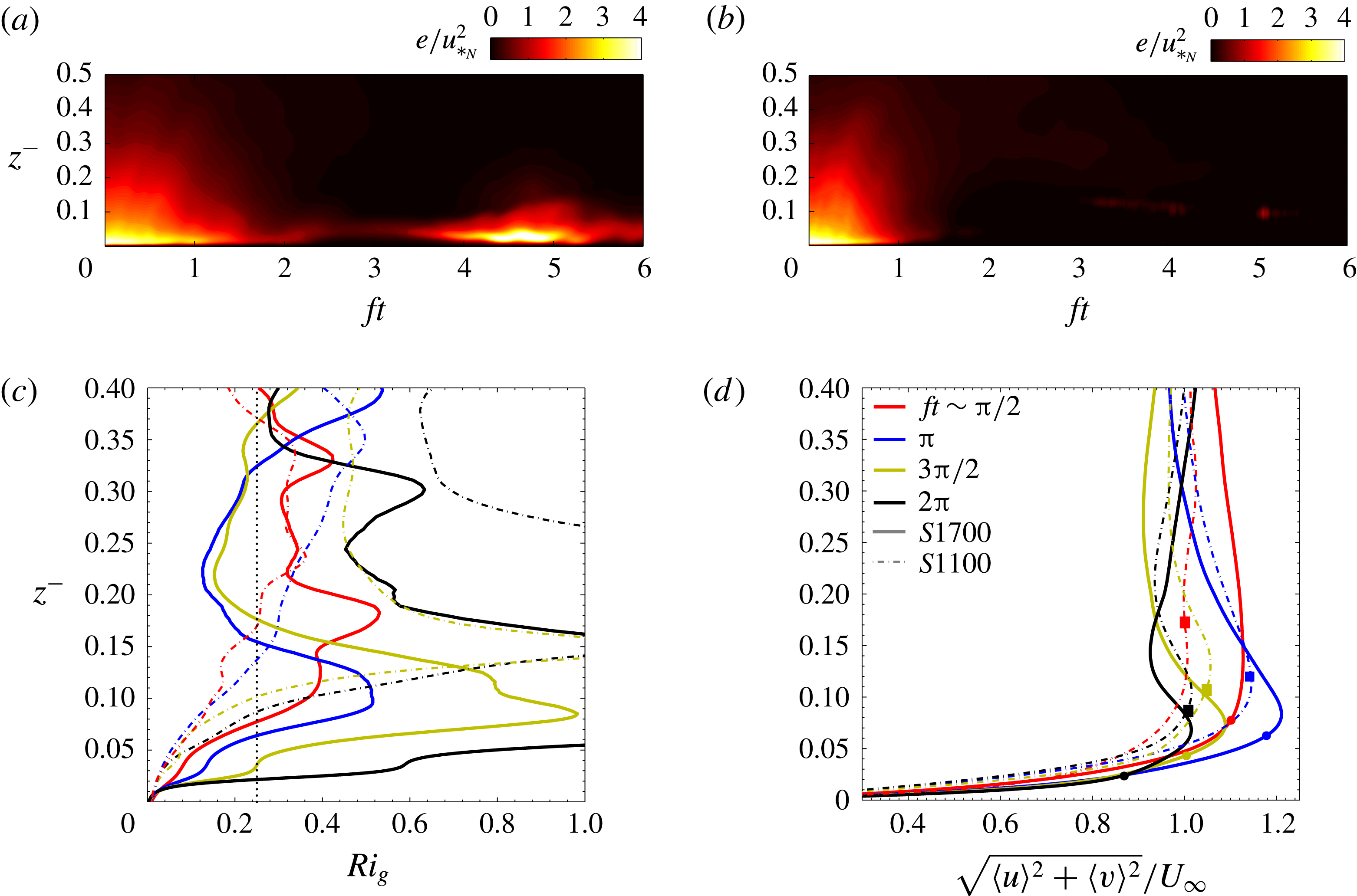
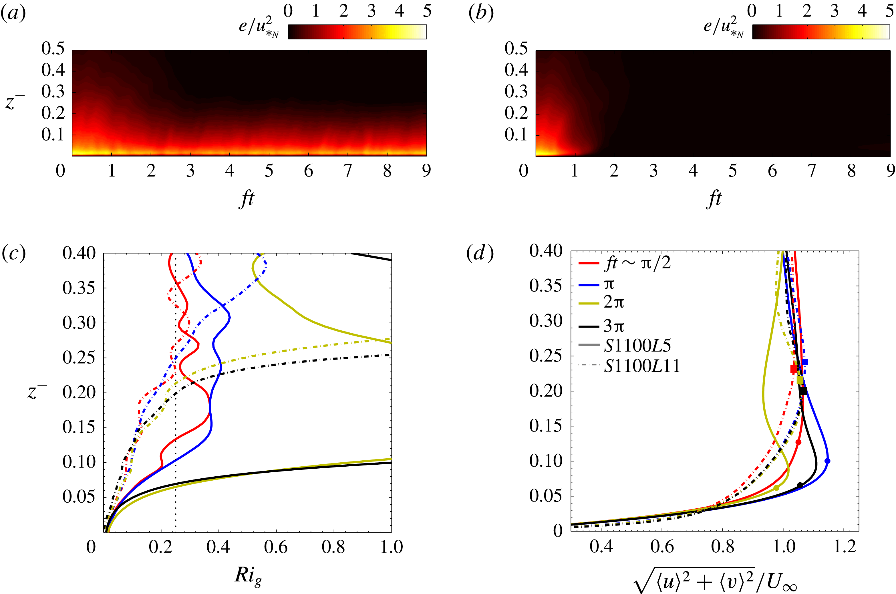
Figure 5(a,b) shows the time–height plot of normalized TKE for case
 $S1100$
and
 $S1700$
, respectively. In case
 $S1100$
, there is virtually no near-surface turbulence during
 $2.5<ft<3.5$
. However, the region between
 $0.05\leqslant z^{-}\leqslant 0.1$
has residual TKE during this period. After
 $ft\approx 3.5$
, near-surface turbulence builds up. The vertical transport of fluctuating energy from the
 $0.05\leqslant z^{-}$
region into the near-surface layers (
 $z^{-}\leqslant 0.02$
) triggers the surface turbulence and leads to eventual recovery as was found by Gohari & Sarkar (Reference Gohari and Sarkar2017) to occur during the turbulence ‘rebirth’ episodes in the Ekman layer subject to constant-flux stability. For case
 $S1100$
, this vertical exchange between outer and inner layers occurs inside a LLJ region which is dynamically unstable. The entire region between
 $z=0$
and the
 $z$
-location of the square symbols on the dashed profiles of figure 5(d) is subcritical with
 $Ri_{g}<0.25$
. Therefore, the LLJ in case
 $S1100$
is receptive to fluctuations transported into that region and rebirth of turbulence is possible. Note that the
 $z$
-location of each square symbol marking the upper boundary of the subcritical region is obtained from the intersection (the first one traversing upward from
 $z=0$
) of the
 $Ri_{g}(z^{-})$
profile in figure 5(c) of the corresponding case with the vertical line at
 $Ri_{g}=0.25$
.
Comparison of early time evolution between case
 $S1700$
and case
 $S1100$
: (a,b) time–height plot of normalized turbulent kinetic energy (
 $e/u_{\ast _{N}}^{2}$
) in case
 $S1100$
and
 $S1700$
, respectively; (c) gradient Richardson number; (d) mean velocity magnitude. The upper boundary of the near-surface layer with
 $Ri_{g}\leqslant 0.25$
is marked with circles in case
 $S1700$
(solid lines) and with squares in case
 $S1100$
(dashed lines).

In contrast with case
 $S1100$
, the sheared lower and upper flanks of the LLJ in case
 $S1700$
have a supercritical value of
 $Ri_{g}>0.25$
that prevents instability even if there is a vertical transport of finite-amplitude fluctuations into the LLJ. Consequently, the near-surface turbulence cannot recover in this case. Although the LLJ in the velocity profile (black solid line of figure 5
d) has strong shear, the stratification is also strong so as to keep
 $Ri_{g}$
above 0.25. Note that the circles on the solid lines of figure 5(d) that mark the upper boundary of the subcritical near-surface region are lower than the nose of the LLJ and their offset from the nose progressively increases with increasing
 $ft$
. Thus, the near-surface layer becomes progressively decoupled from the LLJ mean shear aloft and laminar flow persists.
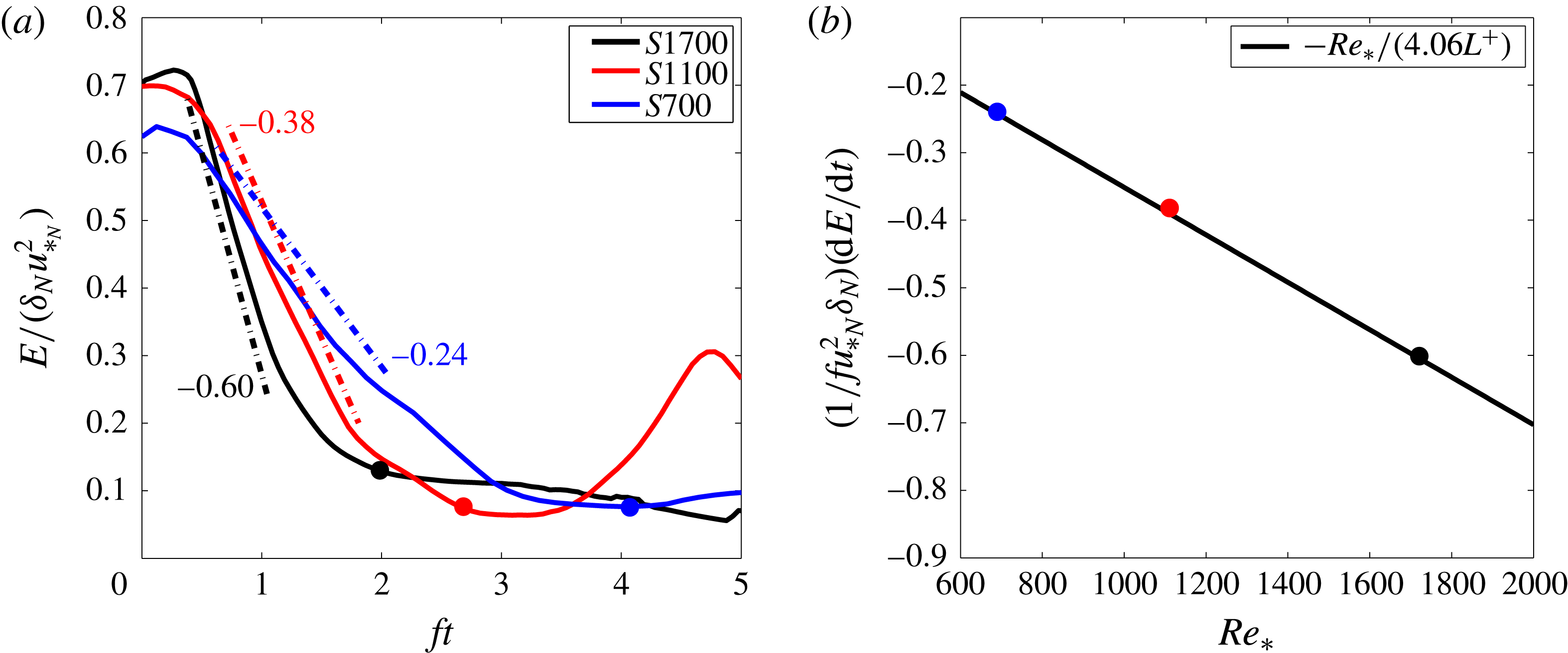
Quantification of the initial collapse of turbulence. (a) The early time evolution of integrated TKE. Each dashed line is a linear fit to the initial decrease of TKE and the adjacent number denotes the slopes of the linear fit. (b) The slopes are plotted as a function of
 $Re_{\ast }$
along with the line that is the best fit to the data.

It is of interest to quantify the dependence of the time interval over which TKE collapses on the parameters
 $L^{+}$
and
 $Re_{\ast }$
in the problem. Figure 6(a) shows that
 $E$
decreases more rapidly as
 $Re_{\ast }$
increases. Furthermore, the initial decrease of
 $E$
is linear. The slope
 $\text{d}E/\text{d}t$
of the linear phase can be used to define a characteristic turbulence-collapse time scale,
 $t_{c}$
, as
 $$\begin{eqnarray}\frac{1}{t_{c}}=-\frac{1}{u_{\ast _{N}}^{2}\unicode[STIX]{x1D6FF}_{N}}\frac{\text{d}E}{\text{d}t},\end{eqnarray}$$
since the initial value of
 $E$
(the height-integrated TKE) is proportional to
 $u_{\ast _{N}}^{2}\unicode[STIX]{x1D6FF}_{N}$
. The stable buoyancy flux introduces a length scale, the Obukhov length
 $L$
and the initial turbulent fluctuations introduce a velocity scale
 $u_{\ast _{N}}$
so that a natural time scale for the buoyancy effect is
 $t_{b}=L/u_{\ast _{N}}$
(Flores & Riley Reference Flores and Riley2011). Now,
 $$\begin{eqnarray}ft_{b}=\frac{fL}{u_{\ast _{N}}}=\frac{Lu_{\ast _{N}}}{\unicode[STIX]{x1D708}}\frac{\unicode[STIX]{x1D708}f}{u_{\ast _{N}}^{2}}=\frac{L^{+}}{Re_{\ast }},\end{eqnarray}$$
where the last of the above equations follows from the definitions of
 $L^{+}$
by (2.6) and
 $Re_{\ast }$
by (2.4c
). We hypothesize that
 $1/ft_{c}$
is proportional to the inverse normalized buoyancy time scale
 $1/ft_{b}$
so that
 $$\begin{eqnarray}-\frac{1}{fu_{\ast _{N}}^{2}\unicode[STIX]{x1D6FF}_{N}}\frac{\text{d}E}{\text{d}t}\propto \frac{Re_{\ast }}{L^{+}}\,.\end{eqnarray}$$
The DNS data presented in figure 6(a) are obtained to compute the left-hand side of (4.4) and, as shown by figure 6(b), the magnitude of the decay rate is found to increase linearly with
 $Re_{\ast }$
in agreement with the prediction of (4.4) for constant
 $L^{+}$
. The coefficient of proportionality is found to be
 $1/4.06$
by linear regression of the DNS data of figure 6(b). Thus, a model for
 $t_{c}$
defined by (4.2) is
 $$\begin{eqnarray}t_{c,\mathit{model}}=4.06\frac{L}{u_{\ast _{N}}}.\end{eqnarray}$$
The corresponding values of
 $t_{c,model}=4.06L/u_{\ast _{N}}$
are denoted in figure 6(a) with circles. It is evident that
 $4.06L/u_{\ast _{N}}$
is a reasonable measure of the time interval required for turbulence to collapse in the simulation. It is worth noting that the DNS data do not show a sharp minimum of
 $E$
so that a precise estimate of the collapse time by the criterion of minimum
 $E$
is not possible.
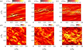
Visualizations of normalized streamwise velocity fluctuation,
 $u^{\prime }/u_{\ast _{N}}$
, near the surface at
 $z^{+}=15$
(a–c) and in the outer layer at
 $z^{-}=0.2$
(d–f), are presented in figure 7 in order to illustrate spatio-temporal intermittency of stratified Ekman flows. These snapshots are taken during the initial decay time period and the corresponding times are indicated using dots in figure 4(b,d,f). Figure 7 indicates that the collapse process does not proceed uniformly in space near the surface, instead, turbulence persists in localized streaks contained within a region where fluctuations have subsided. Thus, there is spatio-temporal intermittency in the near-surface flow wherein turbulence coexists with regions of nearly laminar flow during the temporal decrease of TKE. In contrast, the intermittency is observed to be less strong in the outer layer where turbulence decays in an approximately homogeneous manner , i.e. the turbulent fluctuations in the outer layer are reduced with respect to the neutral case but are not preferentially distributed as streaks. It should be noted that the near-surface streaks are continually evolving and their growth or decay depends on the competition between destabilizing vertical mean shear and stabilizing stratification. For case
 $S700$
and case
 $S1100$
, these structures eventually develop into a spatially extended turbulent state that expands to fill the whole flow domain, however, these structures peter out in case
 $S1700$
and TKE becomes negligible as previously discussed.
Spatial intermittency of near-surface fluctuations in the stratified Ekman layer. Streamwise velocity fluctuations,
 $u^{\prime }/u_{\ast _{N}}$
, on a horizontal plane: (a–c) correspond to a near-surface location,
 $z^{+}=15$
, and (d–f) to an outer-layer location,
 $z^{-}=0.2$
. (a,d) Case
 $S700$
at
 $ft=2.22$
; (b,e) case
 $S1100$
at
 $ft=1.87$
; and (c,f) case
 $S1700$
at
 $ft=1.21$
. The corresponding times are indicated with dots and letters in figure 4. Spatial intermittency refers to near-ground turbulence taking the form of isolated, organized turbulent patches within a background of negligible fluctuations.

The time evolution of: (a) normalized Obukhov scale (
 $L^{+}$
); (b) buoyancy Reynolds number (
 $Re_{b}$
). Case
 $S1700$
has almost zero turbulent dissipation and
 $Re_{b}$
after
 $ft\approx 2$
.

Profiles of statistics at long time against normalized height: (a) normalized velocity; (b) normalized potential temperature (
 $u_{\ast _{N}}(\unicode[STIX]{x1D703}-\unicode[STIX]{x1D703}_{\infty })/q_{0}$
); (c) gradient Richardson number (
 $Ri_{g}$
); (d) normalized variance of temperature fluctuations (
 $u_{\ast _{N}}\unicode[STIX]{x1D703}_{\mathit{rms}}/q_{0}$
); (e) vertical buoyancy flux (
 $\langle w^{\prime }\unicode[STIX]{x1D703}^{\prime }\rangle /q_{0}$
); (f) normalized TKE (
 $e/u_{\ast _{N}}$
). The statistics are averaged during the last
 $ft\approx 2\unicode[STIX]{x03C0}$
.

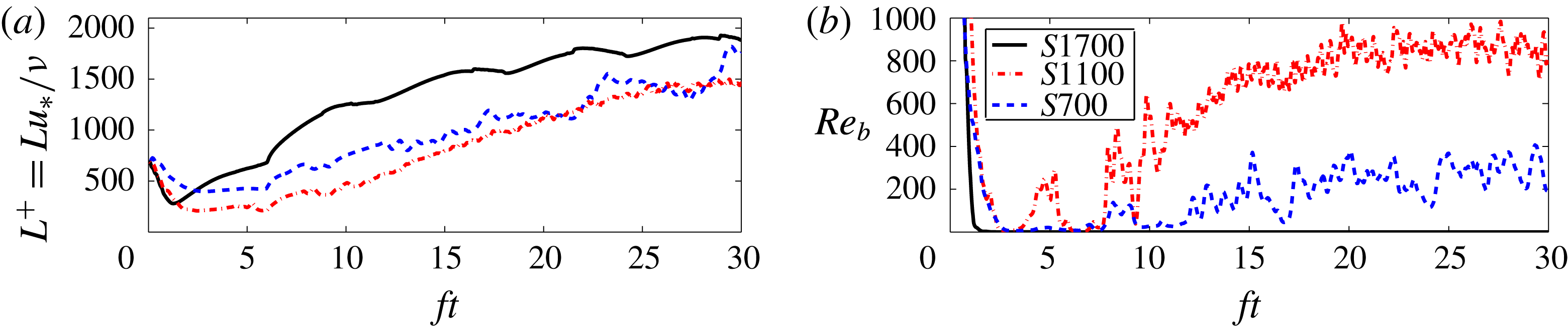
Figure 8(a) illustrates the time series of normalized Obukhov scale. The value of
 $L^{+}$
, initially
 ${\approx}700$
for each case, reaches a minimum value ranging between 200 and 400, similar to the minimum value that is previously reported by Flores & Riley (Reference Flores and Riley2011), Deusebio et al. (Reference Deusebio, Brethouwer, Schlatter and Lindborg2014, Reference Deusebio, Caulfield and Taylor2015). At the point of minimum
 $L^{+}$
, the near-surface fluctuations exhibit spatial intermittency.
 $L^{+}$
eventually increases to values larger than the initial value. Case
 $S1700$
, although having larger
 $L^{+}$
at later times, is non-turbulent. This indicates that, although
 $L^{+}$
can provide guidance as to whether there is an initial turbulence collapse, it does not help predict whether turbulence remains collapsed at long time. The buoyancy Reynolds number,
 $Re_{b}$
, that has been used to distinguish between strong and weak turbulence in stratified flows (Smyth & Moum Reference Smyth and Moum2000; Brethouwer et al.
Reference Brethouwer, Billant, Lindborg and Chomaz2007; Deusebio et al.
Reference Deusebio, Caulfield and Taylor2015) is defined as follows,
 $$\begin{eqnarray}Re_{b}=\frac{\unicode[STIX]{x1D700}}{\unicode[STIX]{x1D708}N^{2}}=\frac{\unicode[STIX]{x1D700}}{U_{\infty }^{2}f}\frac{Re_{\ast }}{Ri_{b}},\end{eqnarray}$$
where
 $\unicode[STIX]{x1D700}$
is the viscous dissipation. An overall value of
 $N^{2}=g\unicode[STIX]{x1D6FC}\unicode[STIX]{x0394}\unicode[STIX]{x1D703}_{0}/\unicode[STIX]{x1D6FF}_{N}$
is assumed to obtain the second equation in (4.6) and the surface value of
 $\unicode[STIX]{x1D700}$
is used in the computation of
 $Re_{b}$
. Figure 8(b) depicts the time evolution of
 $Re_{b}$
. By correlating
 $Re_{b}(t)$
to the fluctuations (TKE and spatial near-surface structures) it is possible to identify critical values of
 $Re_{b}$
that distinguish different flow states in stratified Ekman layers: fully turbulent when
 $Re_{b}\geqslant 180$
, intermittently turbulent when
 $90\leqslant Re_{b}\leqslant 180$
and non-turbulent when
 $Re_{b}\leqslant 90$
. These critical values are similar to the ranges previously reported by Deusebio et al. (Reference Deusebio, Caulfield and Taylor2015) for the boundary between intermittent and fully developed turbulence in stratified plane Couette flow (
 $30\leqslant Re_{b}\leqslant 650$
). It is worth noting that, although these values of
 $Re_{b}$
are helpful in classifying the state of fluctuations in Ekman flows given the value of dissipation rate,
 $Re_{b}$
is a derived turbulence-based quantity. We will explore the suitability of a parameter based on mean flow quantities as a criterion for turbulence recovery in § 4.3.
4.2 Stratified Ekman layer at late time
In the previous section, it was shown that the Ekman flow response to a constant finite-time stabilizing flux with initial
 $L^{+}\approx 700$
includes a decay period with collapsed turbulence and significant changes in the boundary-layer structure. During the decay period, the near-surface region has turbulent streaks in an otherwise quiescent flow. Turbulence recovers in the lower-
 $Re_{\ast }$
cases
 $S700$
and
 $S1100$
but the flow remains non-turbulent at the higher
 $Re_{\ast }=1700$
.
The flow state of the Ekman layer at a late time is quantified . Several statistics are time averaged over the last
 $ft\approx \unicode[STIX]{x03C0}$
of the simulations (
 $27\leqslant ft\leqslant 30$
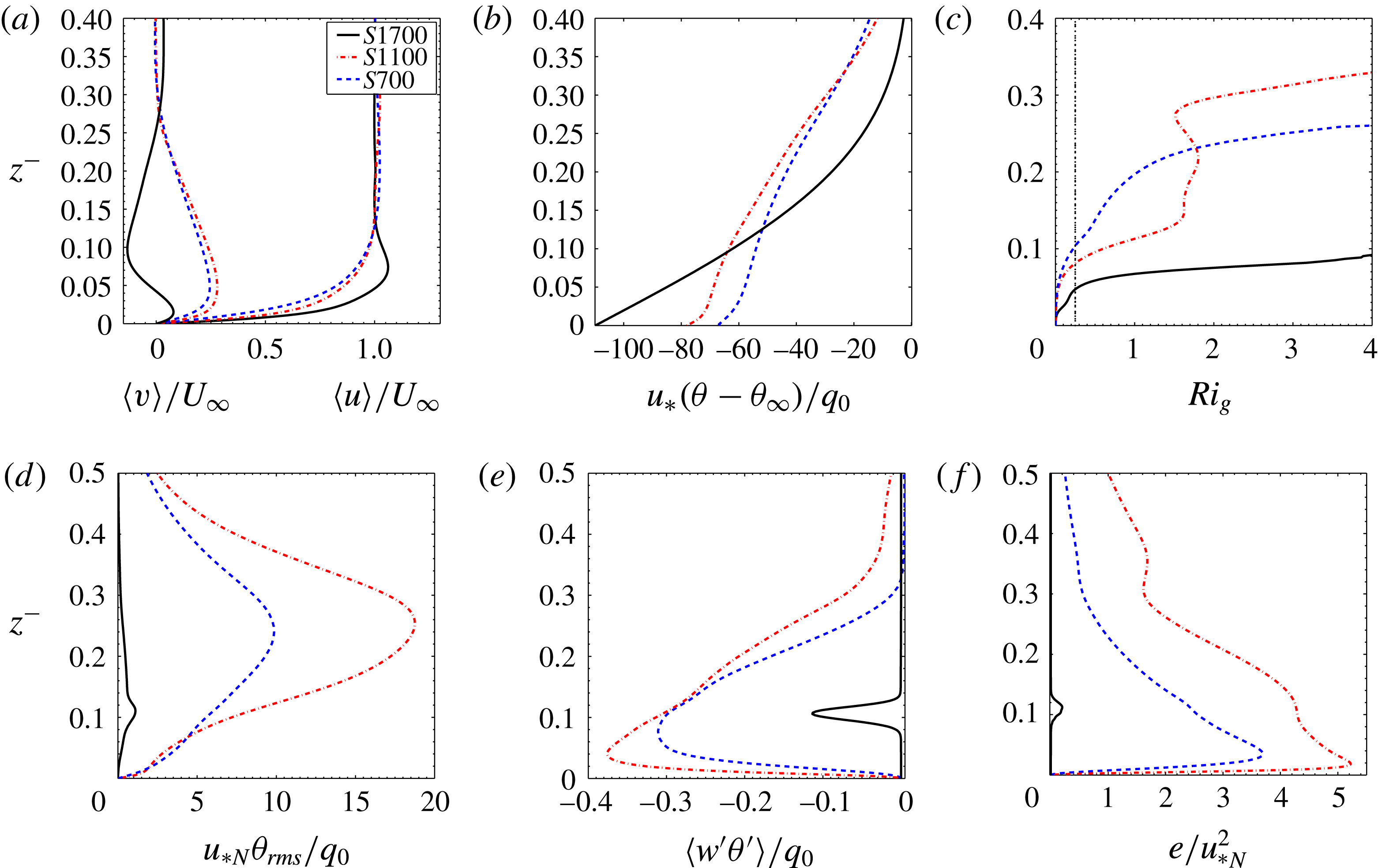
) and the profiles are shown in figure 9. The velocity profiles in case
 $S1700$
(figure 9
a) exhibit the strongest LLJ with an overshoot in the streamwise velocity. The temporal evolution of velocity magnitude shows an LLJ between
 $0.05<z^{-}<0.15$
that oscillates in time (not shown), quite different from the quasi-steady behaviour of the other two stable cases and the neutral reference case. Although all cases develop stable stratification in the near-surface layer, the mean temperature profile (figure 9
b) exhibits quantitative and qualitative differences in the high-
 $Re$
case. Case
 $S1700$
develops the largest stable temperature gradient in the near-surface layer and, furthermore, the temperature varies linearly with height before smoothly merging to the constant-temperature region above. The other cases also have a near-surface layer that has stratification but there is turbulent mixing so that the maximum temperature gradient is not within the near-surface layer but resides above in the capping layer. Despite its stronger LLJ and shear, the strongly stratified inversion in the near-surface layer of case
 $S1700$
leads to a stable region with
 $Ri_{g}>0.25$
that extends from below the LLJ nose (figure 9
c) and is able to decouple the near-surface layer from aloft. In the other two cases, the region with
 $Ri_{g}>0.25$
starts higher up and, therefore, the LLJ has a subcritical
 $Ri_{g}$
allowing for shear instability. The root-mean-square of the temperature fluctuations (figure 9
d) peaks in the thermocline at the location where the temperature gradient also reaches its maximum.
The vertical distribution of TKE is shown in figure 9(f). The TKE profile of case
 $S1100$
has a notably two-layer structure with two local maxima, one below and the other above the LLJ nose level, and a local minimum of TKE at the LLJ nose height. This result is similar to the previous finding of Cuxart & Jiménez (Reference Cuxart and Jiménez2007). It is worth noting that the numerical study of Cuxart & Jiménez (Reference Cuxart and Jiménez2007) was initialized with the velocity and temperature profiles of an observed LLJ in contrast to the present study where the LLJ inherently forms as a response of the Ekman flow to the imposed stabilizing buoyancy flux. Finally, the vertical TKE distribution of case
 $S1700$
shows a non-turbulent near-surface layer with a small amount of fluctuating energy located in the outer region with oscillating LLJ shear (
 $0.05<z^{-}<0.15$
).
We investigated the robustness of the case
 $S1700$
result of a relaminarized boundary layer by conducting a new simulation where random perturbations were added to relaminarized state and examined if the boundary layer remains non-turbulent during its subsequent development. Initial velocity perturbations with fluctuation energy,
 $E/E_{\mathit{neutral}}=0.93$
, and concentrated in a region close to the surface, i.e.
 $z^{-}<0.1$
were added to the flow at
 $ft_{0}\approx 27$
. These fluctuations were generated using the model spectrum,
 $$\begin{eqnarray}E(k)=C\unicode[STIX]{x1D700}^{2/3}k^{-5/3}f_{L}(kL)f_{\unicode[STIX]{x1D702}}(k\unicode[STIX]{x1D702}),\end{eqnarray}$$
where
 $k$
is the spanwise wavenumber,
 $\unicode[STIX]{x1D700}$
is the dissipation rate,
 $\unicode[STIX]{x1D702}$
is the Kolmogorov scale and
 $L=0.5\unicode[STIX]{x1D6FF}_{N}$
. The details of this model spectrum and the non-dimensional functions,
 $f_{L}$
and
 $f_{\unicode[STIX]{x1D702}}$
, can be found in § 6.5.3 of Pope (Reference Pope2000). The magnitude of
 $L$
,
 $\unicode[STIX]{x1D702}$
and
 $\unicode[STIX]{x1D700}$
are taken from the neutral Ekman layer. The time evolution of TKE showed that the initially seeded perturbations were continuously damped and were eventually extinguished by
 $f(t-t_{0})\approx 0.5$
.
4.3 Criterion for recovery
As discussed earlier in § 4.1, although the initial
 $L^{+}\approx 700$
provides a stabilizing flux that is sufficiently strong to cause transient collapse of turbulence, it does not determine the final state of the boundary layer. Turbulence recovers in the lower-
 $Re_{\ast }$
cases
 $S700$
and
 $S1100$
but the flow remains non-turbulent in the higher
 $Re_{\ast }=1700$
case, although the late-time values of
 $L^{+}$
are similar among the cases. From the results of §§ 4.1 and 4.2, it appears that turbulence recovery occurs in the lower-
 $Re$
cases since the
 $Ri_{g}(z)$
profiles have subcritical value in the near-surface layer that allows shear instability to develop. In this section, we investigate how
 $Ri_{b}$
as an alternate choice of overall stratification can provide guidance as to whether turbulence recovers after its initial collapse, by providing a theoretical analysis for the evolution of
 $Ri_{b}$
that shows an increased
 $Ri_{b}$
when
 $Re_{\ast }$
increases at a fixed
 $L^{+}$
, a comparison of such analysis with DNS results, and providing a relation between
 $Ri_{b}$
and average
 $Ri_{g}$
.
Consider the equations governing horizontally averaged quantities denoted by
 $\langle .\rangle$
. Continuity and the impermeability condition leads to the result that
 $\langle u_{3}\rangle (z)$
is identically zero. Averaging of (2.2) over horizontal planes leads to
 $$\begin{eqnarray}\frac{\unicode[STIX]{x2202}}{\unicode[STIX]{x2202}t}\langle \unicode[STIX]{x0394}\unicode[STIX]{x1D703}\rangle +\frac{\unicode[STIX]{x2202}}{\unicode[STIX]{x2202}x_{3}}\langle \unicode[STIX]{x0394}\unicode[STIX]{x1D703}^{\prime }u_{3}^{\prime }\rangle =\unicode[STIX]{x1D706}\frac{\unicode[STIX]{x2202}^{2}}{\unicode[STIX]{x2202}x_{3}^{2}}\langle \unicode[STIX]{x0394}\unicode[STIX]{x1D703}\rangle ,\end{eqnarray}$$
where
 $\unicode[STIX]{x0394}\unicode[STIX]{x1D703}=\unicode[STIX]{x1D703}_{\infty }-\unicode[STIX]{x1D703}$
and superscript
 $^{\prime }$
denotes fluctuation with respect to the average. After using the following boundary conditions:
 $$\begin{eqnarray}\displaystyle & \displaystyle \unicode[STIX]{x2202}\langle \unicode[STIX]{x0394}\unicode[STIX]{x1D703}\rangle /\unicode[STIX]{x2202}x_{3}\rightarrow 0\quad \text{at }x_{3}\rightarrow \unicode[STIX]{x1D6FF}_{N}, & \displaystyle\end{eqnarray}$$
 $$\begin{eqnarray}\displaystyle & \displaystyle \langle \unicode[STIX]{x0394}\unicode[STIX]{x1D703}^{\prime }u_{3}^{\prime }\rangle =0\quad \text{at }x_{3}=0\text{ and }x_{3}=\unicode[STIX]{x1D6FF}_{N}, & \displaystyle\end{eqnarray}$$
 $$\begin{eqnarray}\frac{\unicode[STIX]{x2202}}{\unicode[STIX]{x2202}t}\int _{0}^{\unicode[STIX]{x1D6FF}_{N}}\langle \unicode[STIX]{x0394}\unicode[STIX]{x1D703}\rangle \,\text{d}x_{3}=-\unicode[STIX]{x1D706}\frac{\unicode[STIX]{x2202}}{\unicode[STIX]{x2202}x_{3}}\langle \unicode[STIX]{x0394}\unicode[STIX]{x1D703}\rangle \big|_{0}.\end{eqnarray}$$
Note that
 $q_{0}=-\unicode[STIX]{x1D706}\unicode[STIX]{x2202}_{x_{3}}\langle \unicode[STIX]{x1D703}_{0}\rangle =\unicode[STIX]{x1D706}\unicode[STIX]{x2202}_{x_{3}}\langle \unicode[STIX]{x0394}\unicode[STIX]{x1D703}_{0}\rangle$
is a constant during the application of the constant buoyancy flux in series A. Therefore, integration of (4.10) in time yields
 $$\begin{eqnarray}\int _{0}^{\unicode[STIX]{x1D6FF}_{N}}\langle \unicode[STIX]{x0394}\unicode[STIX]{x1D703}\rangle \,\text{d}x_{3}=-q_{0}t.\end{eqnarray}$$
The left-hand side of (4.11) can be approximated as
 $\langle \unicode[STIX]{x0394}\unicode[STIX]{x1D703}_{0}\rangle \unicode[STIX]{x1D6FF}_{N}/C_{1}$
, where
 $C_{1}$
is a coefficient (
 $C_{1}=2$
, if
 $\langle \unicode[STIX]{x0394}\unicode[STIX]{x1D703}\rangle$
varies linearly with height similar to case
 $S1700$
). Therefore, the equation given in (4.11) becomes
 $$\begin{eqnarray}\langle \unicode[STIX]{x0394}\unicode[STIX]{x1D703}_{0}\rangle \unicode[STIX]{x1D6FF}_{N}=-C_{1}q_{0}t.\end{eqnarray}$$
After substituting (4.12) for the surface temperature into the definition of the bulk Richardson number, (2.9), and using (2.6), we obtain the following expression that describes the initial time evolution of
 $Ri_{b}(t)$
:
 $$\begin{eqnarray}Ri_{b}(t)=C_{1}\frac{u_{\ast _{N}}^{4}}{\unicode[STIX]{x1D705}L^{+}\unicode[STIX]{x1D708}U_{\infty }^{2}}t.\end{eqnarray}$$
The non-dimensional parameters in the problem are the initial Reynolds number (
 $Re_{\ast }$
or
 $Re_{D}=\sqrt{2U_{\infty }/\unicode[STIX]{x1D708}f}$
), the constant buoyancy flux (
 $L^{+}$
) and the time interval (
 $fT$
) over which the buoyancy flux is applied. In order to relate
 $Ri_{b}(t=T)$
to these non-dimensional parameters, (4.13) is rewritten as
 $$\begin{eqnarray}Ri_{b}(T)=C_{1}\frac{fT}{\unicode[STIX]{x1D705}L^{+}}\frac{u_{\ast _{N}}^{4}}{U_{\infty }^{4}}\frac{U_{\infty }^{2}}{\unicode[STIX]{x1D708}f}=C_{2}\frac{fT}{L^{+}}\frac{Re_{D}^{2}}{(\ln Re_{D})^{4}},\end{eqnarray}$$
where
 $$\begin{eqnarray}C_{2}\propto \frac{C_{1}}{\unicode[STIX]{x1D705}}.\end{eqnarray}$$
The second equality of (4.14) is obtained by using the correlation
 $u_{\ast _{N}}/U_{\infty }\approx 1/\ln Re_{D}$
(Coleman et al.
Reference Coleman, Ferziger and Spalart1990).
The time evolution of bulk Richardson number,
 $Ri_{b}$
, in series A. The value of
 $Ri_{b}(ft=6)$
increases with
 $Re_{\ast }$
. Note that in series B to be discussed later in § 5.2, each case has a constant-temperature boundary condition imposed according to the value of
 $Ri_{b}(fT\approx 6)$
of the corresponding series A case.


The time-evolution relation given in (4.14) renders three scenarios under which the bulk stability of the Ekman layer measured by
 $Ri_{b}(T)$
becomes large when one of the three independent parameters
 $\{L^{+},fT,Re_{D}\text{ or }Re_{\ast }\}$
is varied, keeping the other two constant. First, if a stronger stabilizing buoyancy flux (reduced
 $L^{+}$
) is imposed at the surface. Second, if the stabilizing buoyancy flux is imposed for a longer time interval, i.e. larger value of
 $fT$
. Third, if a stabilizing buoyancy flux is imposed at a larger Reynolds number, i.e.
 $Re_{D}$
or equivalently
 $Re_{\ast }$
is increased (the last term in 4.14 monotonically increases with
 $Re_{D}$
). It is the third scenario that applies to DNS series A where
 $Re_{\ast }$
is increased keeping
 $L^{+}$
and
 $fT$
constant. From a physical viewpoint, an increased Reynolds number reduces the viscous scale of the Ekman layer (
 $O(\unicode[STIX]{x1D708}/u_{\ast })$
) and therefore, imposing a stabilizing buoyancy flux based on a constant
 $L^{+}$
(ratio of the Obukhov scale to the viscous scale) yields a reduced buoyancy length scale (
 $L$
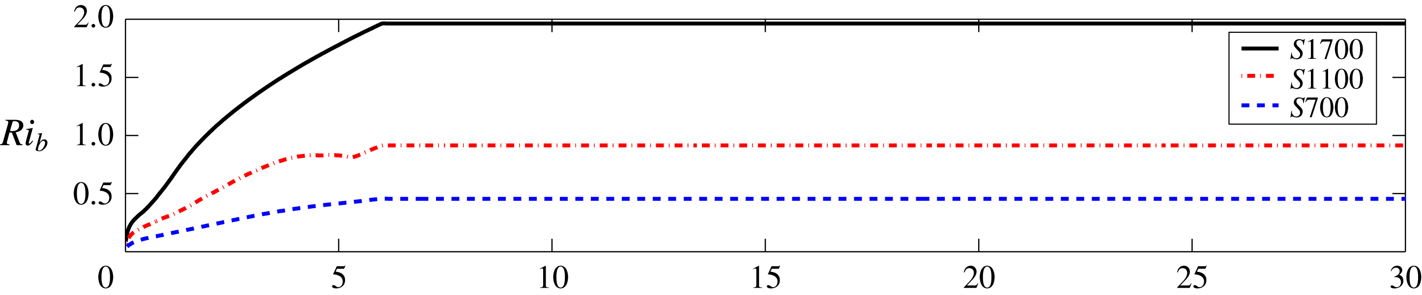
) and a stronger stratification during the flow evolution. In agreement with this analysis, figure 10 shows that the value of
 $Ri_{b}(T)$
at the end of the constant-flux interval of
 $fT\approx 6$
increases with increasing value of initial
 $Re_{\ast }$
in series A.
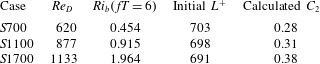
The validity of equation (4.14) for predicting
 $Ri_{b}(fT)$
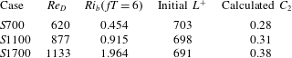
is examined against DNS results. Table 2 summarizes the independent parameters (initial
 $L^{+}$
and
 $Re_{D}$
) for the conducted DNS simulations in series A, as well as the
 $C_{2}$
calculated after inserting
 $Ri_{b}(ft=6)$
and the values of the independent parameters in equation (4.14). The values of
 $C_{2}\approx 0.3{-}0.4$
vary in a narrow range, showing that equation (4.14) with a suitable choice of
 $C_{2}$
, i.e. 0.35, can be used to estimate
 $Ri_{b}(fT)$
prior to the simulation.
An increase in
 $Ri_{b}$
implies a larger value of average
 $Ri_{g}$
as shown below. A vertically averaged value of
 $Ri_{g}$
is introduced as
 $$\begin{eqnarray}\widetilde{Ri_{g}}=\frac{\displaystyle \int _{0}^{L_{z}}N^{2}\,\text{d}x_{3}}{\displaystyle \int _{0}^{L_{z}}S^{2}\,\text{d}x_{3}},\end{eqnarray}$$
where,
 $$\begin{eqnarray}\displaystyle & \displaystyle \int _{0}^{L_{z}}N^{2}\,\text{d}x_{3}=\int _{0}^{L_{z}}\unicode[STIX]{x1D6FC}g\unicode[STIX]{x2202}_{x_{3}}\langle \unicode[STIX]{x1D703}\rangle \,\text{d}x_{3}\approx \unicode[STIX]{x1D6FC}g\langle \unicode[STIX]{x0394}\unicode[STIX]{x1D703}_{0}\rangle , & \displaystyle\end{eqnarray}$$
 $$\begin{eqnarray}\displaystyle & \displaystyle \int _{0}^{L_{z}}S^{2}\,\text{d}x_{3}=\int _{0}^{L_{z}}(\unicode[STIX]{x2202}_{x_{3}}\langle u\rangle ^{2}+\unicode[STIX]{x2202}_{x_{3}}\langle v\rangle ^{2})\,\text{d}x_{3}\approx U_{\infty }^{2}/\unicode[STIX]{x1D6FF}_{N}. & \displaystyle\end{eqnarray}$$
 $$\begin{eqnarray}\widetilde{Ri_{g}}\approx \frac{\unicode[STIX]{x1D6FC}g\langle \unicode[STIX]{x0394}\unicode[STIX]{x1D703}_{0}\rangle }{U_{\infty }^{2}/\unicode[STIX]{x1D6FF}_{N}}=Ri_{b}.\end{eqnarray}$$
Hence, a vertically averaged gradient Richardson number is proportional to
 $Ri_{b}$
, despite the boundary values of
 $Ri_{g}=(\unicode[STIX]{x1D705}L^{+})^{-1}$
at the surface and
 $Ri_{g}=0$
at the top of the layer being constant among the cases of series A. Therefore, an increased value of bulk Richardson number,
 $Ri_{b}$
, increases the average
 $Ri_{g}$
in the Ekman layer (see (4.14) and (4.18)), indicating that there is a greater propensity for supercritical
 $Ri_{g}$
below the LLJ nose (similar to the results of case
 $S1700$
presented in figure 9
a), which prevents instability growth inside the near-surface layer.
5 Discussion
5.1 Extension to high
 $Re$

DNS with the available computational resources is able to provide results for a limited range of Reynolds numbers. We explore the applicability of the DNS results to higher values of
 $Re_{\ast }$
that are not accessible by DNS.
The integrated TKE in the neutral case is proportional to
 $u_{\ast _{N}}^{2}\unicode[STIX]{x1D6FF}_{N}$
. Therefore, increasing the Reynolds number and thereby
 $u_{\ast }$
increases the initial TKE in the boundary layer. Nonetheless, the initial collapse of turbulence is accentuated as
 $Re_{\ast }$
increases in series A as illustrated by figure 6. Equation (4.4) that was derived in § 4.1 showed that the magnitude of the initial decay rate of normalized TKE increases with
 $Re_{\ast }$
for a given
 $L^{+}$
. Therefore, we expect the initial collapse of TKE to be present if
 $Re_{\ast }$
is further increased in series A.
The bulk Richardson number,
 $Ri_{b}$
, was shown to be an average measure of
 $Ri_{g}$
and, therefore, larger
 $Ri_{b}$
indicates a larger propensity for surface-layer values of
 $Ri_{g}(z)$
that are supercritical, thus suppressing shear instability. In particular, case
 $S1700$
with
 $Ri_{b}=1.96$
had supercritical
 $Ri_{g}$
in the LLJ and a non-turbulent final state while case
 $S1100$
had subcritical
 $Ri_{g}$
in the LLJ and turbulence recovered. Equation (4.14) in § 4.3 established that the bulk Richardson number
 $Ri_{b}$
at the end of the period with constant buoyancy flux increased with increasing Reynolds number, i.e. the total extracted buoyancy is larger at a higher
 $Re_{\ast }$
(Williams et al.
Reference Williams, Hohman, Van Buren, Bou-Zeid and Smits2017). Therefore, we expect that the final state will be non-turbulent if the initial Reynolds number in series A is increased beyond
 $Re_{\ast }=1700$
.
5.2 Constant-temperature stability
A new series B of simulations was conducted with constant value of surface temperature and three cases were simulated at
 $Re_{\ast }=692$
, 1112 and 1722, respectively. As described in table 3, each case has the initial
 $Ri_{b}$
chosen to match the value of
 $Ri_{b}(fT\approx 6)$
of the series A case with the corresponding
 $Re_{\ast }$
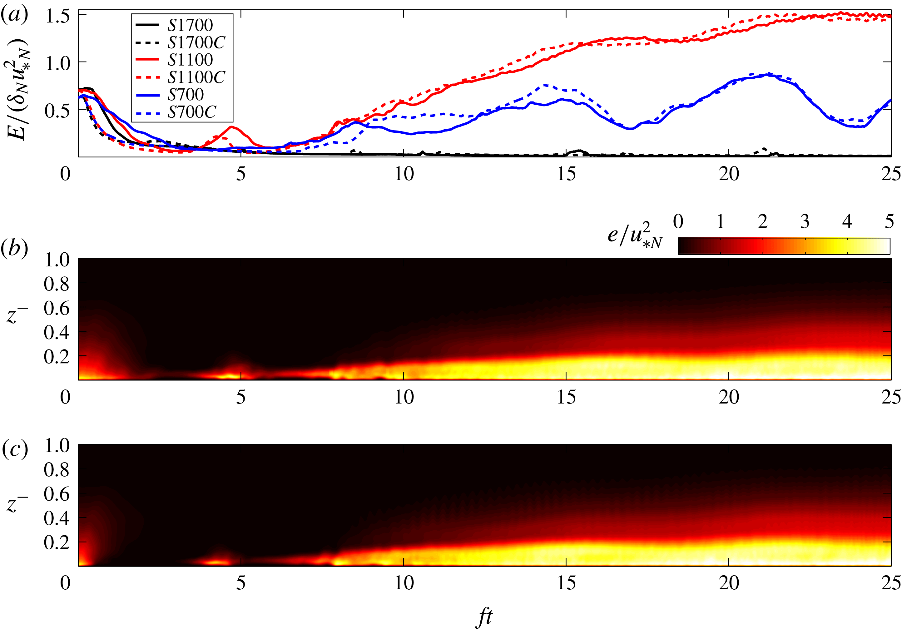
(see figure 10). The objective is to determine the influence of the difference in the surface boundary condition on the early-time and late-time behaviour of stratified Ekman layers. Figure 11(a) shows the time evolution of the integrated TKE for cases in series A (solid lines) and in series B (dashed lines). Generally, the constant-temperature stability results in an earlier collapse of turbulence and an earlier formation of the LLJ. However, after
 $ft=6$
, the difference between corresponding cases of series A and B is small in figure 11(a). The momentum and thermal boundary-layer structures at a late time (not shown here) do not differ significantly from the corresponding cases in series A. Figure 11(b,c), a comparison between time–height plots of normalized turbulent kinetic energy in cases
 $S1100$
and
 $S1100C$
, confirms that there is little difference between corresponding cases of series A and B after
 $ft=6$
. Thus, at each Reynolds number, the nature of the boundary condition used to achieve
 $Ri_{b}(ft=6)$
affects only the initial transient and not the late-time evolution.
The time evolution of integrated turbulent kinetic energy (
 $E/(\unicode[STIX]{x1D6FF}_{N}u_{\ast _{N}}^{2})$
) for cases in series A (solid lines) and series B (dash lines) (a). Time–height plot of normalized turbulent kinetic energy in cases
 $S1100$
(b) and
 $S1100C$
(c).

DNS parameters of simulated cases in series B. In these cases, a constant surface temperature, chosen to match the
 $Ri_{b}(fT\approx 6)$
of cases in series A (see figure 10), is applied at
 $ft=0$
(
 $Ri_{b}$
is constant in time for each case).

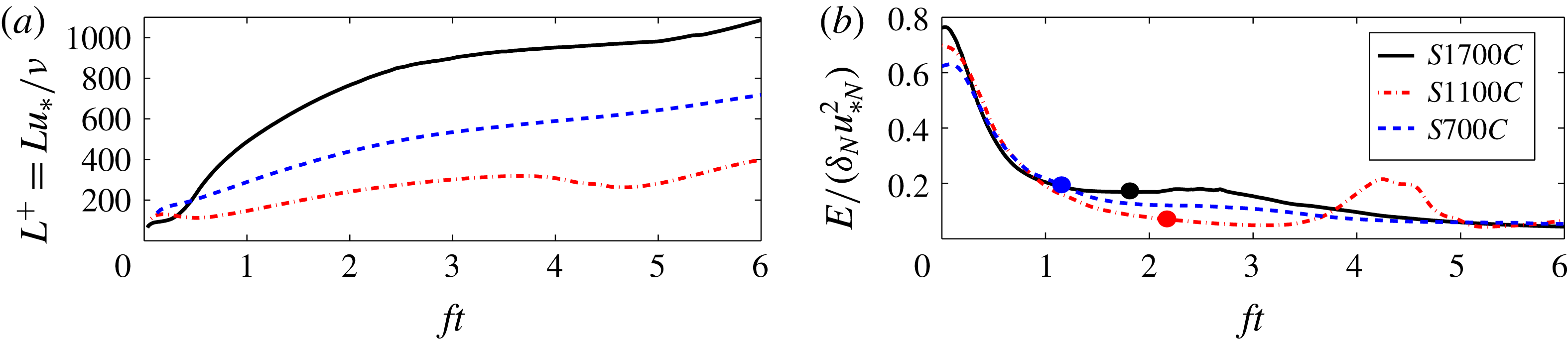
The appropriateness of the model for the turbulence-collapse time scale, discussed in § 4.1 with reference to series A, is now examined for series B. A prediction for the time scale of turbulence collapse is obtained by using the relation given in (4.5) and the
 $L^{+}(ft=0.5)$
value (which is at the end of the ramp-up period, see § 2.3). The corresponding values of the time scale, marked with circles in figure 12(b), exhibit good agreement with DNS results.
The time evolution of: (a) normalized Obukhov scale (
 $L^{+}$
); (b) integrated turbulent kinetic energy (
 $E/(\unicode[STIX]{x1D6FF}_{N}u_{\ast _{N}}^{2})$
) for cases in series B. The time scale for turbulence collapse (computed based on
 $L^{+}$
at
 $ft\approx 0.5$
in (4.5)) are presented with circles in panel (b).

DNS parameters of simulated cases in series C. In these cases, a surface buoyancy flux, chosen to obtain the corresponding
 $L^{+}$
, is applied for a finite time of
 $fT\approx 6$
and then the surface temperature is held constant.

5.3 Effects of initial
$L^{+}$

The effects of initial
 $L^{+}$
on the time evolution of stratified Ekman layers is explored by conducting a new series C of simulations at
 $Re_{\ast }=1112$
with different initial value of
 $L^{+}$
. As listed in table 4, a stabilizing buoyancy flux with the rate of
 $L^{+}\approx 1100$
and
 $L^{+}\approx 500$
are imposed over a time interval of
 $fT\approx 6$
, and the surface temperature is held constant afterwards. The objective is to determine how differences in the initial stabilizing flux affect the transitional behaviour of stratified Ekman layers.
Figure 13(a,b) shows time–height plots of normalized TKE for cases
 $S1100L11$
and
 $S1100L5$
, respectively. In case
 $S1100L11$
, the case with larger initial
 $L^{+}$
compared to case
 $S1100$
, there is no initial collapse and the Ekman layer is continuously turbulent. In case
 $S1100L11$
, almost the entire region of shear is subcritical, i.e. the region with
 $Ri_{g}<0.25$
that lies between
 $z=0$
and the
 $z$
-location of the square symbols on the dashed profiles of figure 13(d) spans the sheared boundary layer. In contrast, case
 $S1100L5$
with a smaller initial
 $L^{+}$
compared to
 $S1100$
, has virtually no turbulence in the boundary layer after
 $ft>2$
. Similar to case
 $S1700$
, the sheared lower and upper flanks of the LLJ in this case have supercritical value of
 $Ri_{g}>0.25$
that prevents the growth of instability (figure 13
d). Consequently, the turbulence ‘rebirth’ episodes in case
 $S1100$
are suppressed in case
 $S1100L5$
. When compared to case
 $S1100$
, the LLJ that is formed in case
 $S1100L5$
is much stronger with an oscillatory behaviour similar to case
 $S1700$
. We expect that an increase in
 $fT$
would have a similar effect as a decrease in initial
 $L^{+}$
(see (4.14)), namely an increased value of
 $Ri_{b}$
at the end of the cooling period so that the flow tends towards stabilization.
Comparison of time evolution between case
 $S1100L11$
and case
 $S1100L5$
: (a,b) time–height plot of normalized turbulent kinetic energy (
 $e/u_{\ast _{N}}^{2}$
) in cases
 $S1100L11$
and
 $S1100L5$
, respectively; (c) gradient Richardson number; (d) mean velocity magnitude. The upper boundary of the near-surface layer with
 $Ri_{g}\leqslant 0.25$
is marked with circles in case
 $S1100L5$
(solid lines) and with squares in case
 $S1100L11$
(dashed lines).

6 Conclusions
Spatio-temporally intermittent Ekman flows are simulated with finite-time stabilizing buoyancy flux, a boundary condition of practical interest that has not been previously investigated using DNS. A buoyancy flux that is temporally constant is applied for a time interval of
 $ft=6$
(comparable to the inertial period of
 $ft=2\unicode[STIX]{x03C0}$
) and then the surface temperature is held constant. The main objectives of this DNS study are: (i) characterization of the initial collapse of turbulence, (ii) quantification of the late-time flow; and (iii) assessment of the flow evolution at different Reynolds numbers.
The parameter that controls the initial collapse of turbulence has been previously suggested to be
 $L^{+}=Lu_{\ast _{N}}/\unicode[STIX]{x1D708}$
based on DNS of stratified open-channel flow (Flores & Riley Reference Flores and Riley2011). Here,
 $L$
is the Obukhov length and
 $u_{\ast _{N}}$
is the friction velocity of the initial neutral boundary layer, and the suggested collapse criterion can be interpreted as the condition at which the dynamic range between the buoyancy-controlled large scale of
 $O(L)$
and the small viscous scale of
 $O(\unicode[STIX]{x1D708}/u_{\ast _{N}})$
is insufficient to sustain turbulence. Our literature survey indicates that the criterion for turbulence collapse is an initial
 $L_{\mathit{cri}}^{+}\approx 700$
which is the lowest initial
 $L^{+}$
for turbulence reported in the field measurements of strongly stable nights (Banta et al.
Reference Banta, Mahrt, Vickers, Sun, Balsley, Pichugina and Williams2007), as well as in simulations of stratified channels (Armenio & Sarkar Reference Armenio and Sarkar2002; Flores & Riley Reference Flores and Riley2011). Simulations with initial
 $L_{\mathit{cri}}^{+}\approx 700$
in series A confirm that there is turbulence collapse irrespective of the variation of Reynolds number
 $Re_{\ast }$
among cases.
Transitional Ekman flow during the initial decay period is found to have spatio-temporal intermittency that appears in the DNS as isolated turbulent streaks near the surface although the turbulence aloft decays in a globally homogeneous manner. These isolated turbulent streaks are identified in an otherwise laminar flow shortly before the completion of the initial collapse of TKE. As discussed by Flores & Riley (Reference Flores and Riley2011), the turbulence of neutral channel flow adjusts to the applied surface buoyancy flux on a time scale of
 $O(L/u_{\ast _{N}})$
. The DNS results show that the adjustment to the imposed surface buoyancy flux in the Ekman layer occurs on a time scale of
 $4.06L/u_{\ast _{N}}$
and the non-dimensional magnitude of the decay rate of vertically integrated turbulent kinetic energy is
 $Re_{\ast }/(4.06L^{+})$
. Moreover, the buoyancy Reynolds number, defined by (4.6), helps distinguish among the different flow states of stratified Ekman flows as follows: turbulent when
 $Re_{b}\geqslant 180$
, strongly intermittent when
 $90\leqslant Re_{b}\leqslant 180$
, and non-turbulent when
 $Re_{b}\leqslant 90$
.
The cases of series A have the same
 $L^{+}\approx 700$
but the Reynolds number,
 $Re_{\ast }$
, ranges between 700 and 1720. Although all cases undergo initial collapse, independent of Reynolds number, the final state varies. The case with highest
 $Re_{\ast }=1720$
develops the highest level of stratification and remains non-turbulent while fluctuations recover in the other cases leading to spatially intermittent turbulence. All the cases have a near-surface layer with subcritical
 $Ri_{g}$
and develop a low-level jet (LLJ) with mean velocity magnitude larger than the geostrophic value. A notable difference at the large
 $Re_{\ast }=1720$
is that the height with a supercritical value of
 $Ri_{g}>0.25$
occurs well below the LLJ which prevents instability in the jet and thus precludes the possibility of the vertical transport of fluctuating energy from the sheared region of the LLJ into the near-surface layer. The LLJ shear is stronger at the large Reynolds number, but the near-surface stratification is also strong leading to supercritical
 $Ri_{g}$
. Our simulations are conducted in a domain of size
 $2\unicode[STIX]{x1D6FF}_{N}\times 2\unicode[STIX]{x1D6FF}_{N}\times 2\unicode[STIX]{x1D6FF}_{N}$
. We were able to conduct new simulations at
 $Re_{\ast }=700$
and
 $1100$
with larger streamwise domain length & different aspect ratio, i.e.
 $4\unicode[STIX]{x1D6FF}_{N}\times 2\unicode[STIX]{x1D6FF}_{N}\times 2\unicode[STIX]{x1D6FF}_{N}$
, to assess sensitivity to domain size. There was little change in the flow evolution and statistics. Nevertheless, it is worth exploring the effect of even larger domain size in future studies.
The initial value of
 $L^{+}$
is the same and its late-time value is similarly large (exceeds 1500) in all cases. Therefore,
 $L^{+}$
does not determine the long-time fate, turbulent or non-turbulent, of the Ekman layer. In series A, the higher-
 $Re$
cases also have larger bulk Richardson number,
 $Ri_{b}$
defined by (2.9), at late time. It is analytically shown that the layer-averaged value of
 $Ri_{g}$
is approximately equal to the bulk Richardson number,
 $Ri_{b}$
. Therefore,
 $Ri_{b}$
is a more suitable parameter than
 $L^{+}$
as an indicator of supercritical
 $Ri_{g}$
in the near-surface layer.
A theoretical analysis is performed to estimate the evolution of
 $Ri_{b}$
during the initial transient of the simulations. Equation (4.14) predicts that when the Reynolds number increases in series A, so should the value of
 $Ri_{b}$
at the end of the constant-flux time interval. Thus the DNS result of series A in figure 10 that the flow relaminarizes at high
 $Re_{\ast }$
(when
 $L^{+}$
is held constant) is an indirect effect of Reynolds number; it is the larger overall stratification as measured by
 $Ri_{b}$
that is responsible for relaminarization. Another prediction of the analysis, see (4.15), is that the final
 $Ri_{b}$
is inversely proportional to
 $L^{+}$
for constant Reynolds number. Results of a new series C of simulations, conducted at constant
 $Re_{\ast }\approx 1100$
and varying
 $L^{+}$
relative to its value of 700 in series A, are in agreement with this prediction. Moreover, an increase of the imposed buoyancy flux to
 $L^{+}=500$
results in a qualitative change: stratification becomes so large (final
 $Ri_{b}=1.45$
) that the lower and upper flanks of the LLJ become supercritical and turbulence rebirth is suppressed. It is also worth noting that when the initial buoyancy flux is decreased to
 $L^{+}=1100$
, turbulence does not collapse at any time during the subsequent evolution of the flow.
The field measurements of strongly stable nights by Banta et al. (Reference Banta, Mahrt, Vickers, Sun, Balsley, Pichugina and Williams2007) demonstrate a fully decoupled near-surface layer with suppressed turbulence for a long period of time. The coupling between the near-surface layer and the outer layer is found to be especially weak during nights with large
 $Ri_{b}$
, e.g. during the night of October 26 during the CASES-99 observational campaign when
 $Ri_{b}$
exceeded 2. The ABL studies of Banta et al. (Reference Banta, Mahrt, Vickers, Sun, Balsley, Pichugina and Williams2007) and Cuxart & Jiménez (Reference Cuxart and Jiménez2007) refer to two layers of TKE with a local minimum in between at the nose of the LLJ which agrees with our results for case
 $S1100$
(see figure 9). Thus, the findings of the present DNS of an idealized configuration are relevant to the stratified ABL.
Both constant-temperature and constant-flux boundary conditions have been employed in previous work. The influence of the method whereby stratification is imposed is studied by conducting series B where constant temperature is imposed in each case rather than constant surface buoyancy flux so as to get the same stability (quantified by final
 $Ri_{b}$
) of the corresponding case in series A. A comparison between series A and B of the mean and turbulence profiles indicate minor differences after
 $ft\approx 6$
. Insofar as the initial transient, cases of series B exhibit an earlier collapse of turbulence relative to series A.
Acknowledgements
We gratefully acknowledge the support of NSF grant CBET-1306869. This work used the Extreme Science and Engineering Discovery Environment (XSEDE), which is supported by National Science Foundation grant no. ACI-1548562.