For more than two decades, political scientists have created statistical models aimed at generating out-of-sample predictions of presidential elections. In 2004 and 2008, PS: Political Science and Politics published symposia of the various forecasting models prior to Election Day. This exercise serves to validate models based on accuracy by garnering additional support for those that most accurately foretell the ultimate election outcome. Implicitly, these symposia assert that accurate models best capture the essential contexts and determinants of elections. In part, therefore, this exercise aims to develop the “best” model of the underlying data generating process. Scholars comparatively evaluate their models by setting their predictions against electoral results while also giving some attention to the models' inherent plausibility, parsimony, and beauty.
Our approach is different. Rather than creating the best model or theory, instead we create an ensemble prediction of the upcoming election. We combine the intuition, theories, and concepts implicit in all of the forecasting models presented in this symposium to make an accurate out-of-sample prediction. Without arbitrating between models and theories, we aim to aggregate them solely with an eye toward increasing our chances of getting it right.
To do this, we rely on the models presented in this issue. We believe that each model captures an important set of insights about US elections. Our approach combines those insights into a single ensemble prediction. For our purposes, the theoretical differences between the models are irrelevant. All that matters is that each provides predictions for previous elections that we can use to evaluate their accuracy. We then weight each forecast by its previous performance and combine them to create the most accurate out-of-sample forecast possible that also captures the uncertainty and diversity inherent in these models.
ENSEMBLE BAYESIAN MODEL AVERAGING
Our approach, ensemble Bayesian model averaging (EBMA), improves out-of-sample forecasting by aggregating across models and originated in the field of weather forecasting (Raftery et al. Reference Raftery, Gneiting, Balabdaoui and Polakowski2005). EBMA builds on the assumption that there exists no “best” model for predicting outcomes of complex systems like the weather or presidential elections. For instance, some weather models might better predict “normal” weather patterns while others better forecast rapidly changing conditions. By averaging across multiple prediction models, EBMA improves forecast accuracy without attempting to select the “best” model.
EBMA evaluates the predictive performance of its component models in a calibration period to generate a weight for each model. Roughly speaking, EBMA creates a weighted average of the predictions made by each of the components.Footnote 1 In particular, the EBMA model gives more weight to more accurate component models, as well as those models that make more unique predictions.Footnote 2 One advantage of EBMA is that it relies on predictions from each component model rather than the full set of covariates and estimated coefficients. Thus, it is possible to include forecasts generated from any kind of process including subject experts, classification trees, or agent-based models.
MATHEMATICAL INTUITION
More technically, EBMA works in the following way.Footnote 3 Assume we have an outcome y t* in the future that is to be predicted and k forecasting models (M 1,M 2,…, M k). The probability of each predictive model capturing the true data-generating process comes from a prior distribution, and one can describe y t in terms of its probability density function (PDF) conditional on M k. Applying Bayes' rule, we derive the marginal predictive distribution of y t* given the k predictive models as
 $$
p(y^{t*} ) = \sum\limits_{k = 1}^K {p(y^{t*} |M_k )p(M_k |y^t ).}
$$
This PDF can be interpreted as a weighted prediction, where the weights of each model M k are dependent on the predictive performance in the calibration period prior to t*.
Each forecasting model is associated with a PDF, which in our case is a normal density function centered at the individual forecast N(f kt*,σ2). The predictive distribution for observation y 2012 (or our forecast for 2012) is then,
 $$
Vote_t = \alpha + \beta _1 \left( {\sum\limits_{j = 0}^{14} {\lambda ^j \Delta \ln R_{t - j} \cdot \left( {{1 \over {\sum\nolimits_{j = 0}^{14} {\lambda ^j } }}} \right)} } \right) + \beta _2 \;Fatalities_t
$$
where w k represents the weight associated with each component model. We estimate weights via maximum likelihood methods.Footnote 4
The basic insight of the EBMA approach is that each component model in the ensemble captures some understanding of the world that is selectively accurate. Combining and weighting these by their past predictions creates a meta-model that, in principle, yields out-of-sample forecasts that are as accurate as any individual component model in terms of predictive accuracy and precision. Across many elections, the ensemble will likely dominate each of its members. Indeed, past research shows that EBMA performs well in a variety of settings such as inflation (Gneiting and Thorarinsdottir Reference Gneiting and Thorarinsdottir2010; Koop and Korobilis Reference Koop and Korobilis2009; Wright Reference Wright2009), economic growth (Billio et al. Reference Billio, Casarin, Van Dijk and Ravazzolo2010; Brock, Durlauf, and West Reference Brock, Durlauf and West2007), exchange rates (Wright Reference Wright2008), industrial production (Feldkircher Reference Feldkircher2012), and weather (Berrocal et al. Reference Berrocal, Raftery, Gneiting and Steed2010; Chmielecki and Raftery Reference Chmielecki and Raftery2010; Raftery et al. Reference Raftery, Gneiting, Balabdaoui and Polakowski2005). Its theoretical underpinnings, as well as its success in a variety of empirical contexts, suggest it could be useful in predicting presidential elections.
THE EBMA FORECAST FOR 2012
To apply EBMA to presidential election forecasting, we use the calibration-period predictions of each component model to estimate the model weights. Here, we use predictions generously provided by Abramowitz, Berry and Bickers, Campbell (Trial-Heat Model), Cuzán (FPRIME-short), Erikson and Wlezien, Hibbs, Holbrook, Lewis-Beck and Tien (Jobs Model), Lockerbie, and Norpoth and Bednarczuk from the models described in this symposium. This results in an ensemble of 10 forecasting models and a training period of 16 presidential elections from 1948 to 2008. Our test period is, of course, the 2012 election.
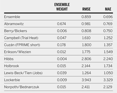
Table 1 shows the EBMA model statistics for the calibration period—the estimated weights for each individual model, the root mean squared error (RMSE), and the mean average error (MAE) for the calibration period spanning the postwar era. All of the component models receive some weight in the final ensemble, although the weights are far from uniform. Abramowitz's model, based on June 2012 polling data, second-quarter GDP growth in the election year, and the presence of a first-term incumbent (adjusting for polarization), receives the lion's share of the predictive weight. In contrast, EBMA heavily down-weights both the Hibbs and Lockerbie models.
Ensemble Weights and Fit Statistics for Calibration-Period Performance (1948–2008)

The second column contains the weight assigned to each component model in the final ensemble. The other columns show two fit statistics to evaluate the relative performance of each component model and the ensemble across the calibration period. EBMA tends to place higher weight on better performing models, but the relationship is not monotonic.
These weights should not be interpreted to indicate that some models are “better,” but only that the EBMA procedure found this mix to provide the highest rate of calibration-sample predictive accuracy while still reflecting a realistic level of predictive uncertainty. Nor should too much emphasis be placed on the individual performance of models, as the causes may be different for each. The EBMA model generally places the greatest weight on models that use polling data (e.g., Abramowitz), while it gives much less weight to models that offer no predictions for much of the calibration period (e.g., Berry and Bickers) or those based on data measured far in advance of the election (e.g., Hibbs).
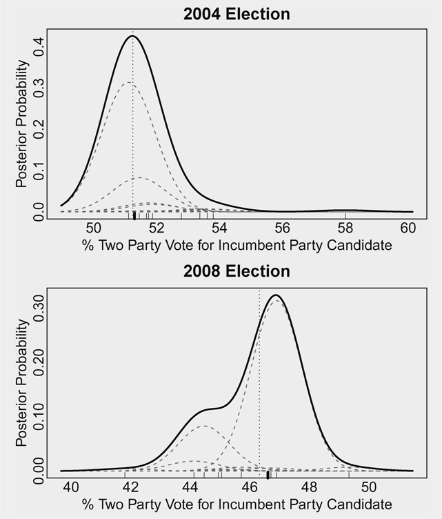
Figure 1 provides a visual representation of the kinds of predictive PDFs generated by EBMA. The figure displays the PDFs of our EBMA model for 2004 and 2008 (in-sample) as bold lines, and the predictive densities of the component models in the ensemble as dashed lines. (The latter have been scaled by the model weights.) It shows the point predictions of each component (light dashes) and the ensemble model (bold dash) at the bottom of each plot.
EBMA Posterior Distributions for the 2004 and 2008 Elections (in-sample)
The dashed curves show the component PDFs and the solid curve shows the final EBMA PDF. The light dashes at the bottom show the point predictions of each component, the bolded dash shows the EBMA posterior median, and the vertical dotted line shows the actual election outcome.

These two plots show that for any given year, EBMA may not necessarily produce the predictions closest to the actual result (shown as a vertical dotted line), although it comes close. Across many elections, however, EBMA tends to outperform its component models in accuracy while also reflecting the uncertainty implied by the different predictions of the component models.
With our EBMA model in hand, we create our ensemble forecast for 2012. Taking the weights reported in table 1 and the forecasts provided by the respective authors, we estimate that the vote for the Democratic candidate for the 2012 US presidential election will be 50.3% with a 95% credible interval ranging from 46.4% to 52.5%. According to the EBMA posterior, President Obama will win the majority of the popular vote with 0.60 probability. Thus, the collective wisdom of this crowd of models—or at least their wisdom as we have combined them—is that 2012 will be a close election but that President Obama has a slight, but non-trivial, edge in the popular vote.
CONCLUSION
Combining different sets of information is a time-honored tradition of many who forecast important elections. Pundits and scholars regularly aggregate polls or expert opinions when trying to glimpse the future. Ensemble methods, as briefly presented and applied here, provide a principled way to weight each component of such aggregations based on accuracy. This approach collates the good parts of existing models while avoiding over-fitting. It aims for greater accuracy as both the knowledge and implied uncertainty of a variety of approaches are integrated into a combined probability distribution. One aspect of our approach that is relatively unique in the extant literatures on presidential vote forecasting (but see Bartels and Zaller Reference Bartels and Zaller2001) is that it accentuates not only our predictions of election outcomes but also our estimate of the uncertainty around those predictions. Neither the literature nor the popular press emphasizes estimates of predictive uncertainty, and too often they do not even report them. Our uncertainty is part of our knowledge and merits full reporting and evaluation.
The summer of 2012 has seen an increased level of attention to political scientists' ability to do “non-lousy” forecasting (Stevens Reference Stevens2012). The irony is that forecasting per se has never been at the heart of social science, despite claims to the contrary. Therefore, we emphasize that our ensemble depends on the insight contained in all of the individual components. In the end, mere predictive accuracy cannot substitute for substantively oriented research. Forecasting serves as an additional heuristic, one normally demanded of scientific endeavors wherein a replication of results in a new situation is expected to produce the same findings. This predictive heuristic can improve our models by showing us where they break down, as well as where they stand strong.
Thus, the predictive enterprise works collectively and individually to improve understanding of the political world. Keeping score for both the individual models and the forecasting literature as a whole tells us if we are improving. Note, therefore, that in the one area in which there is some track record of political science forecasting, namely the prediction of the US presidential elections, the well-known models perform fairly well by some measures. For example, the average absolute error in-sample is about 1.6%. This is not perfect by any stretch of the imagination, but hardly lousy. Indeed, the diversity of models, as well as their accuracy, has improved over time.
We cannot guarantee that our ensemble estimate is the most accurate in the 2012 election. The future is full of surprises, and we only have a small number of relevant elections on which to construct our ensemble estimates. However, given what we know about the performance of these 10 models of presidential voting, we derive an estimate in which we place a high degree of confidence: between 46.4% and 52.5% of the US voters will support the incumbent in 2012, and there is a 0.60 probability that the vote for Obama will be greater than 50%.
ACKNOWLEDGMENTS
We thank Alan Abramowitz, Michael Berry and Kenneth Bickers, James Campbell, Alfred Cuzán, Robert Erikson and Christopher Wlezien, Douglas Hibbs, Thomas Holbrook, Michael Lewis-Beck and Charles Tien, and Brad Lockerbie, as well as Helmut Norporth and Michael Bednarczuk for generously sharing their data with us for this enterprise. All their contributions are described in detail elsewhere in this symposium, but are not herein separately indexed.