1. INTRODUCTION
We consider estimation of the long-memory parameter d for a stationary process {Yt : t = 1,…, n}. The spectral density of the time series is given by

where d ∈ (−0.5, 0.5) is the long-memory parameter and g(·) is an even function on [−π,π] satisfying 0 < g(0) < ∞. The parameter d determines the long-memory properties of the process {Yt}, and g(λ) determines its short-run dynamics. To maintain generality of the short-run dynamics of {Yt}, we do not impose a specific functional form on g(λ). Consistent with the literature on narrow-band semiparametric estimation of the long-memory parameter, we only assume certain regularity conditions for g(λ) near frequency zero.
Examples in the literature of the narrow-band approach include the widely used log-periodogram (LP, also known as the GPH estimator) regression estimator, introduced by Geweke and Porter-Hudak (1983) and further analyzed by Robinson (1995b) and Hurvich, Deo, and Brodsky (1998), and the local Whittle estimator (LW, also known as the Gaussian semiparametric estimator), suggested by Künsch (1987) and further studied by Robinson (1995a). These narrow-band approaches approximate ln g(λ) by a constant in a shrinking neighborhood of the origin. As a consequence, these estimators achieve a rate of mean-squared error (MSE) convergence of only n−4/5, no matter how regular g(λ) is. In addition, these estimators can be quite biased in finite samples because of contamination from high frequencies (see Agiakloglou, Newbold, and Wohar, 1993). Given these problems, Andrews and Guggenberger (2003) and Andrews and Sun (2004) propose approximating ln g(λ) locally by an even polynomial of degree 2r. This leads to the bias-reduced log-periodogram estimator

of Andrews and Guggenberger and the local-polynomial Whittle estimator

of Andrews and Sun. The main feature of these estimators is that for g(·) smooth in a neighborhood of zero, the bias generally converges to zero at a faster rate than that achieved by the GPH and local Whittle estimators. The bias improvement however comes at the price of an increase in the asymptotic variance by a multiplicative constant cr, for example, c1 = 2.25 and c2 = 3.52.
In this paper, we introduce modified versions of the GPH and local Whittle estimators that we denote by

, respectively. These estimators are given as a weighted average over finitely many GPH (or a k-step version of the local Whittle) estimators

calculated using different bandwidths mi. The bandwidth set is of the form {[li m]}i=1K, for

. The idea of the weighted estimator is to choose weights wi in such a way that the r dominant bias terms of the underlying GPH (or k-step local Whittle) estimator are eliminated. Building on results in Hurvich et al. (1998), Robinson (1995a, 1995b), Andrews and Guggenberger (2003), and Andrews and Sun (2004), we derive the asymptotic bias, variance, and MSE of the weighted estimators and establish their asymptotic normality. Our asymptotic results imply that, if the weights wi are chosen appropriately, the weighted estimator shares or even improves on the asymptotic bias advantage of the estimators of Andrews and Guggenberger and Andrews and Sun. The main advantage of the weighted estimator over the estimators of Andrews and Guggenberger and Andrews and Sun is that the multiplicative constant cr by which the asymptotic variance is inflated can be chosen to be arbitrarily small. In other words, the new estimator can be designed to have the asymptotic bias properties of the estimators of Andrews and Guggenberger and Andrews and Sun but its asymptotic variance properties are better. Under local smoothness assumptions on g, the weighted estimator can be designed such that the order of the asymptotic bias gets arbitrarily close to the parametric one, whereas at the same time its asymptotic variance can be made smaller than the asymptotic variance of the GPH (or local Whittle) estimator.
By choosing the weights appropriately, we can obtain an estimator that has the same asymptotic bias as the Gaussian semiparametric estimator but a smaller asymptotic variance. Robinson (1995a, p. 1640) conjectures that ¼ is the semiparametric efficiency bound for the estimation of the long-memory parameter for a given sequence of bandwidths, say, m, and that the Gaussian semiparametric estimator achieves this bound. See also Hidalgo (2005) for further discussion of this issue. Our results do not contradict Robinson's conjecture, as the weighted estimator uses information beyond bandwidth m. However, our results do imply that it is possible to design a more efficient estimator than

while maintaining or even reducing its asymptotic bias. Most existing narrow-band estimators are based on only one bandwidth m. In contrast, the weighted estimator is based on several bandwidths by averaging over the estimators

over a set of li's.
Apart from the theoretical properties, the weighted estimators are also computationally attractive. Both

(the latter estimator being based on a k-step version of the local Whittle estimator) require only K ordinary least squares (OLS) regressions and one generalized least squares (GLS) regression. This is an advantage over the procedure in Andrews and Sun (2004) that requires a nonlinear optimization routine to calculate the estimator.
The weighted estimator depends on the choice of the parameters r,m, and l. From results in Andrews and Guggenberger (2003) it follows that for a fixed l, the optimal choice of r and m in terms of the rate of convergence of the estimator depends on the unknown smoothness of g at zero. We provide an adaptive estimator of d (denoted AWLW for “adaptive weighted local Whittle”), based on Lepskii (1990), that uses the data to select r and m. We show that this estimator obtains the optimal rate of convergence up to a logarithmic factor. We suggest rule of thumb choices for the sequence l based on the relative performance of the weighted estimator in a Monte Carlo study.
In Monte Carlo simulations, using various models including one with nonsmooth spectrum, we compare the root mean-square error (RMSE) performance of the AWLW estimator with several other adaptive estimators, namely, with the ones in Giraitis, Robinson, and Samarov (2000), Hurvich (2001), Iouditsky, Moulines, and Soulier (2001), and Andrews and Sun (2004). The results are very encouraging and show that if the contamination from the short-run component of the spectrum is not too large, the AWLW estimator typically outperforms the other adaptive estimators in RMSE performance.
Besides Andrews and Guggenberger (2003) and Andrews and Sun (2004), another bias reduction approach in the narrow-band literature is that of Robinson and Henry (2003), who consider a general class of semiparametric M-estimators of d that utilize higher order kernels to obtain bias reduction. As they state, their results are heuristic in nature, whereas the results in our paper are established rigorously under specific regularity conditions. Also, their estimators suffer from a variance inflation that can be very large.
An alternative to the narrow-band approach to bias reduction is the so-called broad-band approach where one imposes regularity conditions on g over the whole interval [0,π] and one utilizes a nonparametric estimator of g(λ) for λ ∈ [0,π]. Examples include Moulines and Soulier (1999, 2000), Hurvich (2001), Hurvich and Brodsky (2001), Iouditsky et al. (2001), and Hurvich, Moulines, and Soulier (2002). In these papers, ln g(λ) is approximated by a truncated Fourier series. It is established that under the given regularity conditions the estimators exhibit an asymptotic MSE of order (ln n)/n provided the number of parameters in the model goes to infinity at a suitable rate.
From a broad perspective, the weighted estimator bears some similarity to the generalized jackknife estimator in the kernel smoothing literature. In that literature, it has been suggested to average kernel estimators over different smoothing parameters to achieve bias reduction (see, e.g., Gray and Schucany, 1972; Härdle, 1990, Sec. 4.6).
We now quickly mention possible extensions of the paper. Although we focus on scalar time series satisfying (1.1), it should be possible to extend the idea to the multivariate case along the lines of Robinson (1995b) and Lobato (1999). Although our results are obtained for stationary processes, they can also be utilized when the underlying process is nonstationary (see the discussion in Andrews and Sun, 2004, p. 571). In this case, a preliminary consistent estimator, such as the estimator of Kim and Phillips (1999a, 1999b), Velasco (1999), Velasco and Robinson (2000), Phillips and Shimotsu (2004), or Shimotsu and Phillips (2005), is required. Although the asymptotic results for the weighted Whittle estimator are derived without assuming Gaussianity, we require such an assumption for the weighted log-periodogram estimator. Using the insight of Velasco (2000), the assumption of Gaussianity could possibly be relaxed for the latter estimator also. Finally, rather than averaging over different

or (a k-step version of)

estimators as in this paper, we could apply the weighted approach to

or (a k-step version of)

for r ≥ 1 to eliminate additional bias terms. These extensions however are beyond the scope of this paper.
The remainder of this paper is organized as follows. In the next section, we review the estimators of Andrews and Guggenberger (2003) and Andrews and Sun (2004) and lay out the assumptions. Section 3 introduces the new weighted estimators and establishes their asymptotic properties. Section 4 discusses adaptive estimation. Section 5 describes the simulation results, and the Appendix provides proofs of the theorems.
By Cs(U) we denote the space of functions that are s-times continuously differentiable on the open set U. By [s] we denote the integer part of

. For a matrix A we denote by [A]i,. and [A]i,j the ith row and the (i,j)th element of the matrix A, respectively, and 1(·) is the indicator function.
2. THE LOG-PERIODOGRAM AND WHITTLE ESTIMATOR
In this section we review the bias-reduced log-periodogram regression estimator

of Andrews and Guggenberger (2003) and the local-polynomial Whittle estimator

of Andrews and Sun (2004). These estimators are used as benchmarks for later comparisons. We also lay out the assumptions.
For

define


The bias-reduced log-periodogram estimator

is the least squares estimator of d from the pseudo-regression of ln Ij on a constant, −2 ln λj,λj2,…, λj2r−2, and λj2r for j = 1,…, m, where m is the number of fundamental frequencies employed in the regression. The estimator is based on the identity derived from (1.1):

where, if defined,

are the first terms of the Taylor series expansion of ln(gj /g0), C := 0.57721 … is the Euler constant, and

are regarded as regression errors. The GPH estimator is obtained by setting r = 0 and is based on approximating ln(gj /g0) by a constant around the origin.1
More precisely, instead of −2 log λj, the original GPH estimator was defined using log|1 − exp(−iλ)| as the regressor for d. For the asymptotic statements given in our theorems, this difference is of no importance.
For notational convenience we typically suppress the dependence of the estimator on r and/or m and write

for

.
The local-polynomial Whittle estimator

of Andrews and Sun (2004) is an M-estimator that minimizes the (negative) local-polynomial Whittle log-likelihood. The latter is given by

where the notation G := g0 is taken from Robinson (1995a) and Andrews and Sun (2004) and

Concentrating Qr(d,G,b) with respect to G ∈ (−∞,∞) yields the concentrated local-polynomial Whittle log-likelihood

:

The local-polynomial Whittle estimator

of (d,b) solves the following minimization problem:

where Θ is a compact and convex set in

. Existence and uniqueness of

hinge on strict convexity of

(see Andrews and Sun, 2004, p. 576) and convexity and compactness of the parameter space. The local Whittle estimator (Künsch, 1987; Robinson, 1995a) is obtained by setting r = 0.
Before we state the assumptions we need the following definition. We say that a real function h defined on a neighborhood of zero is “smooth of order 0 < s < ∞ at zero” if h ∈ C[s](U) for some neighborhood U of zero and its derivative of order [s], denoted h([s]), satisfies a Hölder condition of order s − [s] at zero; that is, |h([s])(λ) − h([s])(0)| ≤ C|λ|s−[s] for some constant C < ∞ and all λ ∈ U. We say that h is “smooth of order ∞ at zero” if h is smooth of order s for every finite s.
Andrews and Guggenberger (2003) make the following assumptions to derive the asymptotic properties of the log-periodogram estimator

.
Assumption AG1. f (λ) = |λ|−2dg(λ), where d ∈ (−½,½).
Assumption AG2.
(a) g is smooth of order s ≥ 2 + 2r at λ = 0 for some nonnegative integer r.
(b) g is an even function on [−π,π], 0 < g(0) < ∞, and

.
Assumption AG3. The time series {Yt : t = 1,…, n} is Gaussian.
Assumption AG4. m = m(n) → ∞ and m/n → 0 as n → ∞.
For the local-polynomial Whittle estimator Andrews and Sun (2004) make the following assumptions.2
Note that we do not include Assumption 3(b) in Andrews and Sun (2004) in our AS3. It is used in Robinson (1995a) to obtain a law of large numbers for εt2 without fourth-moment assumptions. But AS3(a) yields this law of large numbers because it implies that εt2 − 1 is a bounded variance martingale difference sequence.
In AS4 note the following. If s > 2 + 2r is assumed as in AG2, Assumption 4 in Andrews and Sun (2004) boils down to m0.5+2r/n2r → ∞ and m2.5+2r/n2+2r = O(1) as n → ∞. If we want to be certain that in (2.10) τr b2+2r m2+2r/n2+2r is the dominant higher order bias expression, we have to sharpen assumption m2.5+2r/n2+2r = O(1) to m2.5+2r/n2+2r → χ ∈ (0,∞) in AS4. The reason is that m2.5+2r/n2+2r = O(1) is compatible with m2.5+2r/n2+2r = o(1), in which case it is not clear that τr b2+2r m2+2r/n2+2r is the dominant higher order bias expression: there could be other op(1) terms that converge to zero more slowly than τr b2+2r m2+2r/n2+2r.
Assumption AS1. Assumption AG1 holds for d ∈ [d1,d2] with −½ < d1 < d2 < ½.
Assumption AS2. Assumption AG2 holds.
Assumption AS3.
(a) The time series {Yt : t = 1,…, n} satisfies

where

and Ft−1 is the σ-field generated by {εs : s < t}.
(b) In some neighborhood of the origin, (d/dλ)α(λ) = O(|α(λ)|/λ) as λ → 0+, where

.
Assumption AS4. AG4 holds, and m2.5+2r/n2+2r → χ ∈ (0,∞) as n → ∞.
Under Assumptions AG1–AG4, Theorem 1 in Andrews and Guggenberger (2003) gives the following formulas for the asymptotic bias and variance of the

estimator.
3In the discussion of the local Whittle estimator, we mean by “asymptotic bias” the difference of the mean of the asymptotic distribution of the estimator and the true value of d. In contrast, for the log-periodogram estimator, “asymptotic bias” refers to the asymptotic behavior of

. For technical reasons, we cannot use this definition for the Whittle case. The same comment applies to “asymptotic variance.” For further discussion of the difference of these two concepts refer to Davidson and MacKinnon (1993, p. 124).


If s = 2 + 2r, then the O(mq/nq) term can be replaced by o(mq/nq). The numbers τr and cr are defined in Andrews and Guggenberger, for example, τ0 = −2.19, τ1 = 2.23, τ2 = −0.793 and c0 = 1, c1 = 2.25, and c2 = 3.52.
If in addition AS4 is assumed, which asymptotically is the MSE-optimal choice of m, Andrews and Guggenberger (2003, p. 687, Com. 2) show that4
If m2.5+2r/n2+2r = o(1) then

, and similar modifications hold for the other asymptotic normality results that follows. We focus on the case m2.5+2r/n2+2r → χ ∈ (0,∞) in our discussion because this is the MSE-optimal growth rate for m.

or equivalently that

Similarly, under AS1–AS4, Andrews and Sun (2004) show that for the

estimator

Comparing the bias of

with that of

, one sees that the rate of convergence of the bias to zero is generally faster for the former, whereas its variance is increased by the multiplicative constant cr. When ln g(λ) is approximated reasonably well by ln g0 in a neighborhood of zero, the bias reduction for

over

may be very small, and the increase in variance may dominate the reduction of bias in finite samples. It would be desirable to have an estimator that shares the asymptotic bias properties of the estimators of Andrews and Guggenberger (2003) and Andrews and Sun (2004) without inflating the asymptotic variance or at least inflating it by a constant smaller than the constant cr. In the next section, we describe a new estimator for d that has these properties.
3. WEIGHTED SEMIPARAMETRIC ESTIMATORS
In this section, we introduce the new weighted estimator

and investigate its asymptotic properties. We first describe its general form as a weighted average of an estimator

at different bandwidths m and then explicitly look at the cases e = LP and e = LW. More precisely, rather than using the local Whittle estimator

, we work with a k-step local Whittle estimator

defined in (3.12), which follows. The k-step estimator is computationally more attractive than the local Whittle estimator (because it is given in closed form) but shares its relevant asymptotic properties.
To motivate the weighted estimator, consider the

estimator at two different bandwidths m1 and m2 that are given as multiples of m for fixed numbers li, mi := [li m], i = 1,2. Recall that under certain regularity conditions and rate conditions on m, the asymptotic bias of the log-periodogram estimator can be written as

Define a weighted estimator

by

It follows from (3.1) that the asymptotic bias of

is of order o(m2/n2) because by choosing weights w2 := m12/(m12 − m22) and w1 := −m22/(m12 − m22) we have eliminated the dominant bias terms of

. By choosing l1 and l2 appropriately, we can in addition control the asymptotic variance of

. In the following discussion we describe how to design weights and pick constants li such that the weighted estimator has the same asymptotic bias as

but smaller asymptotic variance.
The example illustrates the idea of the weighted estimator. We now consider the general case in which the average is taken over more than two different bandwidths and higher order biases may be eliminated. To describe it, let r (as in

) be a nonnegative integer that denotes the number of dominant bias terms to be eliminated, l = (l1,l2,…, lK)′ be a K-vector that pins down the different bandwidths
5Without loss of generality, we impose lj > lj−1, and for convenience, we always pick l such that the increments lj+1 − lj are equal, for j = 1,…, K − 1. Furthermore, m and lK are picked such that [lK m] ≤ n/2. Assuming that l is a vector with rational components li = pi /qi (for relatively prime integers pi and qi and i = 1,…, K) and that m contains all the qi as factors, it follows that mi = li m. To simplify the exposition, we make this assumption from now on. Of course, all the results go through without this assumption. For example, take the bias formula in Theorem 3.2: because mi2k/m2k = li2k + O(1/m), condition (3.3) implies that for k = 1,…, r we have

, which is dominated by O((ln3 m)/m).

, and finally w = (w1,w2,…,wK)′ be a K-vector of weights that satisfies


Occasionally, we impose an additional condition on the weights, namely,

The weighted estimator is then defined by6
To simplify notation, we do not explicitly list K and w among the parameters that the weighted estimator depends on. The dependence on K is implicit through l, and in the text we describe a procedure of how to pick w given r, m, l, and δ.

where in Sections 3.1 and 3.2 we will explicitly focus on the cases e = LP and e = LW. If

is only subject to conditions (3.2) and (3.3) then of course

.
We now discuss conditions (3.2)–(3.4). Condition (3.2) guarantees that

is asymptotically unbiased. Condition (3.3) is motivated from Lemma 3.1(i), which follows. Lemma 3.1(i) states that the asymptotic bias of the log-periodogram estimator up to lower order terms is given by

for some constants τk*. Therefore, the condition implies that the highest order bias terms of

up to m2r/n2r are eliminated for

. Under (3.2) and (3.3), we occasionally want to be able to control the multiplicative constant for the resulting dominant bias term m2+2r/n2+2r of the weighted estimator. For example, in this section we match the dominant bias term of

with that of

and then compare their asymptotic variances to deduce the superiority of the weighted procedure in terms of MSE. Condition (3.4) pins down the multiplicative constant of the dominant bias term through appropriate choice of δ. Condition (3.4) is imposed mainly to make the bias/variance comparison of the weighted procedure with other estimation methods. In Section 4 we will implement the adaptive weighted estimator based solely on conditions (3.2) and (3.3).
Note that conditions (3.2)–(3.4) are invariant to renormalization of the vector l. More precisely if r,m,l,δ satisfy conditions (3.2)–(3.4) then so does r,Lm,l/L,δ for any positive constant L, and we have

. Therefore, without loss of generality we can normalize l1 = 1. It should be noted that when δ is chosen to match the asymptotic bias of

with that of

, as in Theorem 3.2, which follows, it is no longer innocuous to normalize l1 = 1. Nevertheless, we will use the normalization l1 = 1 for the remainder of the paper unless otherwise stated.
Subsequently we give some theory and Monte Carlo–based discussion and rules of thumb of how to choose the parameters r,m,l, and δ. For now, we take these parameters as given and describe an easy procedure to implement

, that is, a procedure to design weights w satisfying conditions (3.2)–(3.4). The implementation without condition (3.4) is analogous. Consider the following pseudo-regression of

on a constant,

:

where ui is the error term. Note that the regression coefficients β stand for different quantities in the cases e = LP and e = LW. For notational convenience however, we use β in both cases. Let

The weighted estimator

of d is defined as the first component of the GLS estimator of (d,β) = (d,β2,β4,…, β2+2r), that is,

where

and

is the K-vector with ith element

. In Lemma 3.1(ii), which follows, we establish that up to a multiplicative constant Ω is the asymptotic variance matrix of u = (u1,…,uK). It is easy to see that

is a weighted average of the

with weights given by

These weights satisfy conditions (3.2)–(3.4) and give rise to our weighted estimator

.
In the Sections 3.1 and 3.2, we analyze the properties of the weighted estimator

when the components of

are the log-periodogram regression estimator

or a k-step version of the local Whittle estimator

. Both of these estimators are easy to compute. For example, for the estimator

we only need to first run K OLS regressions to get

and then one GLS regression (3.7) to obtain

.
3.1. The Weighted Log-Periodogram (WLP) Estimator
We now consider the weighted estimator

in (3.7) when e = LP. The asymptotic properties of

depend crucially on those of

and the covariance structure of

. We first state the following refinement of the results of Theorem 1 in Hurvich et al. (1998).
LEMMA 3.1. Suppose Assumptions AG1–AG4 hold. Then,
(i) The bias of

satisfies

where

and q is defined in (2.7). If s = 2 + 2r the O(mq/nq) term can be replaced by o(mq/nq).
(ii) The covariance between

is given by

The lemma shows that we can actually ignore the o(·) term in the asymptotic bias formula (2.6). This is crucial when proving the next theorem, which is a corollary of the lemma.
THEOREM 3.2. Let r and l be fixed constants and

for some τ ≠ 0. Then, under Assumptions AG1–AG4, we have

where the O(mq/nq) term can be replaced by o(mq/nq) if s = 2 + 2r.
Remarks.
(a) If lim(m/nκ) ∈ (0,∞) for 1 > κ > (2 + 2r)/(3 + 2r), then the dominant bias term of

is τb2+2r m2+2r/n2+2r. From (2.6), the dominant bias term of

is τr b2+2r m2+2r/n2+2r. Therefore, the asymptotic biases of the two estimators converge to zero at the same rate. In particular, the rate is quicker than that of the GPH estimator if r > 0 and b2 ≠ 0.
(b) Suppose lim(m/nκ) ∈ (0,∞) for some 0 < κ < 1 and the assumptions of Theorem 3.2 hold. Then the asymptotic MSE (AMSE) of

satisfies

If κ > (2 + 2r)/(3 + 2r), then the O(·) term in (3.9) is of smaller order than the other two terms. Ignoring the O(·) term and assuming that τ2b2+2r2 ≠ 0, minimization of

with respect to m gives the AMSE-optimal choice of m:

Note that the AMSE-optimal growth rate of n(4+4r)/(5+4r) allows one to ignore the O(·) term in (3.9). The bandwidth mopt depends on the unknown b2+2r. Guggenberger and Sun (2003) propose a plug-in method to estimate mopt.
(c) To compare the asymptotic properties of

, we choose τ = τr, which makes the dominant bias terms of the two estimators equal. Table 1 demonstrates that l can be chosen such that the constant cr* in the asymptotic variance of

is smaller than cr, that is, although having the same asymptotic bias properties, the asymptotic variance properties of the new estimator are better than those of

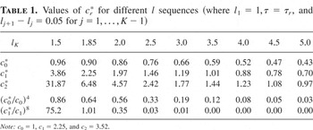
. We have cr* = cr for r = 0 and r = 1 if lK = 1.2 and lK = 1.85, respectively, and for larger choices of lK, the weighted estimator has smaller asymptotic variance than the corresponding

estimator in Andrews and Guggenberger (2003) with same asymptotic bias. In comparison with the GPH estimator

, the estimator

can be designed such that it improves (if r > 0 and b2 ≠ 0) or retains (if r = 0) the asymptotic bias and at the same time reduces the asymptotic variance.
Values of cr* for different l sequences (where l1 = 1,τ = τr, and lj+1 − lj = 0.05 for j = 1,…, K − 1)

(d) From numerical results such as the ones reported in Table 1, we conclude that for each r and ε > 0, l can be chosen such that cr* ≤ ε. Therefore, asymptotic theory suggests that larger values of lK in the definition of

imply better variance properties, whereas the asymptotic bias can remain unchanged. This is not surprising because by Lemma 3.1(ii) larger l values deliver log-periodogram estimates with smaller variance. Therefore, there is no trade-off in the asymptotic bias and variance for the choice of lK. However, in finite samples larger values for lK have a negative effect on the bias properties of

, that is, just as for the bandwidth m, there is a bias/variance trade-off when choosing l in finite samples. The reason for the negative effect is that the approximation of ln(gj /g0) by its Taylor polynomial b2 λj2/2 + ··· + b2+2r λj2+2r/(2 + 2r)! can be very poor for large values of j. Large values for l imply large values for the mi, and the bias reduction does not work as well as for smaller values of l.
(e) It might seem unfair to compare

with

because the latter estimator is based on more frequencies lK m and therefore is expected to have a smaller variance. However, note that

(implemented using τ = τr) has the same dominant higher order bias as

and that increasing m in

—while reducing its asymptotic variance—would increase its asymptotic bias. It therefore follows that in terms of asymptotic

is dominated by

for appropriate choices of the vector l. To make this statement formal, let m* be the AMSE-optimal bandwidth for

. Andrews and Guggenberger (2003, eqn. (3.17)) show that under weak regularity conditions m* is given by

where the positive number A is defined as

Ignoring higher order terms and using equation (3.19) in Andrews and Guggenberger (2003), the resulting optimal AMSE of

is then given by

for

This is the smallest AMSE that

can achieve as a function of m. In particular, note that using a larger bandwidth, say, m*lK for some lK > 1, would only make the AMSE bigger.
Now, compare the preceding results to what we obtain for

, using the same bandwidth m = m* used before and

. The choice of δ ensures that

has the same dominant higher order bias as

; see equation (2.6) and Theorem 3.2. Up to higher order terms, equation (3.9) states that

for

As reported in Table 1, cr* < cr for appropriate choices of l1,…, lK, and hence W* < W. Therefore,

, when implemented with the AMSE optimal choice m* of

, has smaller AMSE than

. Clearly, if we used

with its AMSE optimal choice mopt given in (3.10), the AMSE advantage would only become larger.
(f) The same point about the superiority of the weighted estimator

over the estimator

in terms of AMSE can be made by making the asymptotic variances of the estimators equal and then showing that the asymptotic bias of the weighted estimator is smaller.
7We thank a referee for pointing out this alternative approach to showing the AMSE superiority of the weighted estimator.

(up to higher order terms) we have to choose the bandwidth m* for the weighted estimator such that cr*/m* = cr /m or m* = (cr*/cr)m.
8More precisely, m* = [(cr*/cr)m], but this difference does not matter for what follows.

differs from that of

by the factor (cr*/cr)4+4r. The last two rows of Table 1 show that this factor can be made smaller than 1 for appropriate choices of lK. For example, for lK = 2.5 the factor (cr*/cr)4+4r equals 0.33 and 0.03 for r = 0 and r = 1, respectively. This proves again that, compared to

, the weighted estimator can be implemented such that its AMSE is smaller: although it has the same asymptotic variance, it has smaller (squared) bias. The title of the paper is inspired by this way of looking at the superiority of the weighted estimator.
Using the results of Hurvich et al. (1998), Robinson (1995b), and Andrews and Guggenberger (2003), we now establish the asymptotic normality of

.
THEOREM 3.3. Under the assumptions of Theorem 3.2 and AS4, we have

For r ≥ 1, the assumptions of the theorem allow one to take m much larger than for the asymptotic normality result for the GPH estimator (compare to Hurvich et al., 1998, Thm. 2). Therefore, by choosing m appropriately, one has asymptotic normality of

with a faster rate of convergence than is possible with

. This feature is also obtained for the estimator

. The difference between

is that the asymptotic variance of the latter estimator is smaller than that of the former estimator when l is chosen such that cr* < cr.
3.2. The Weighted Local Whittle (WLW) Estimator
In this section, we investigate the properties of the weighted estimator

defined in (3.7) when e stands for a k-step local Whittle estimator

. We show that for given r ≥ 1,

can be constructed to share the higher order bias advantages of

but offers the additional advantage of a smaller variance than

and computational simplicity.
We first introduce the k-step estimator

and motivate its choice. As shown in the Appendix (see (A.6) and Lemma A.2 for r = 0), for each k ≥ 1,

has the same asymptotic N(0,¼) distribution as the local Whittle estimator

defined in (2.5) but has a closed form expression. Hence, although sharing its relevant theoretical properties,

has computational advantages over

. Although in our simulations that follow we take k = 1, we give the theory for general k ≥ 1.
For notational convenience, we write

(; see equation (2.4). Let

be the normalized first (score) and second (Hessian) derivatives of

, respectively. Define

where X*(m) is an m-vector with jth element Xj*(m) given by

For notational simplicity, we usually write Xj* for Xj*(m). The k-step (Gauss–Newton-type) local Whittle estimator is defined recursively by9
We could also define a k-step (Newton–Raphson-type) local Whittle estimator by the recursion

, for j = 1,2,…, k, where we use the same notation as in (3.12). We use Jm instead of

because it is technically more convenient and computationally simpler as Jm does not depend on any estimated parameter. We have not formally established the equivalence of the Newton–Raphson and Gauss–Newton procedures in terms of the results of the paper.

where

is an

-consistent estimator of d. For example, we can define

.
Let

be the K-vector with ith element

. The weighted local Whittle estimator

is obtained by replacing

in equation (3.7) by

, that is,

Note that in the notation we suppressed the dependence on r,m,l, and δ. Using Lemma A.2 in the Appendix, the following theorem can be proved.
THEOREM 3.4. Let r and l be fixed constants and

for some τ ≠ 0. Then under Assumptions AS1–AS4, we have

for

defined in (A.21) in the proof of the theorem, for example,

.
Remarks.
(a) The asymptotic bias of

equals (τ/τr*)Dr m2+2rn−(2+2r) and is thus of order m2+2rn−(2+2r). Therefore, for r > 1, the asymptotic bias is smaller than that of

by an order of magnitude; recall that for

the asymptotic bias is of order m2/n2. Furthermore, using the weighted version

of the local Whittle estimator

changes the asymptotic variance by the multiplicative constant cr*. If cr* is smaller than 1, then the asymptotic variance of the weighted estimator is smaller than that of

.
(b) The estimator

can be modified to have the same dominant asymptotic bias term as

. More specifically, define

for consistent estimators

. Guggenberger and Sun (2003, Prop. 11) give examples of such estimators. Then, under the assumptions of Theorem 3.4 we have

Therefore, the estimator

has the same dominant asymptotic bias term τr b2+2r m2+2rn−(2+2r) as

but asymptotic variance depending on cr* rather than cr. If l is chosen appropriately, we can have cr* < cr (see Table 1), implying that

has better asymptotic variance properties than

. In consequence,

has the same asymptotic advantage over

, that is, the same asymptotic bias but smaller asymptotic variance, as

has over

. Note that there is no clear advantage of

over

. The adjustment in (3.14) may increase or decrease the asymptotic bias of

, depending on the values of

.
(c) It follows from Table 1 that we can choose l such that c0* < 1. Therefore, the weighted estimator

has the same asymptotic bias as the Gaussian semiparametric estimator

but smaller asymptotic variance. An unproven conjecture states that the Gaussian semiparametric estimator attains the semiparametric efficiency bound (Robinson, 1995a, p. 1640). Our result does not constitute a contradiction to this belief, because the efficiency of the Gaussian semiparametric estimator is conjectured for a fixed sequence of bandwidths, whereas

is based on an average over a number of different bandwidths.
(d) Results in Andrews and Guggenberger (2003) and Andrews and Sun (2004) show that

have the same dominant bias term τr b2+2r(m/n)(2+2r). In contrast, Theorems 3.2 and 3.4 imply that the dominant bias terms τb2+2r(m/n)(2+2r) and (τ/τr*)Dr(m/n)(2+2r) of the weighted estimators

are different for r ≥ 1 with the difference depending on b.
(e) Assume that lim(m/nκ) ∈ (0,∞) for some 0 < κ < 1. It follows that under the assumptions of Theorem 3.4 the asymptotic MSE of

is given by

The AMSE-optimal choice of m is thus given by

A plug-in method to estimate mopt has been proposed in Guggenberger and Sun (2003).
4. ADAPTIVE ESTIMATION
The estimator

depends on the choice of r and m, the number of dominant bias terms to be eliminated and the bandwidth, respectively.
Using the plug-in method suggested in Hurvich and Deo (1999) and also used in Andrews and Guggenberger (2003), one can choose m to minimize the asymptotic MSE of the estimator of d for given r and s large enough. The formulas for the optimal m in (3.10) and (3.15) depend on the unknown parameter b2+2r or Dr The plug-in method replaces the unknown parameter by a consistent estimate and can be adapted to our situation (see Guggenberger and Sun, 2003). However, this method has several drawbacks. First, it is not fully automatic because it depends on a first-stage regression where one has to make an initial choice of the bandwidth. Second, because r is assumed fixed, the method does not adapt to the local smoothness of the spectrum at zero, and therefore, in general, the MSE convergence of the estimator to zero is not rate optimal.
In this section, we therefore choose a different route that adapts the choice of r and m to the smoothness of the spectrum at zero. The basic method for this approach comes from Lepskii (1990) and has been used in the context of estimation of the long-memory parameter by Giraitis et al. (2000), Iouditsky et al. (2001), Hurvich et al. (2002), and Andrews and Sun (2004).
According to our previous definition of “smooth of order s at zero,” a function that is smooth of order s1 is also smooth of order s2 whenever s1 > s2. The rate optimal choice of r is an increasing function of the smoothness of the spectrum at zero, and we are therefore interested in determining the “maximal degree s0 of smoothness at zero.” In the following discussion we first precisely define the quantity s0 and then describe a procedure to consistently estimate it. More precisely, we use the weighted local Whittle estimator to design a consistent estimator

of s0. As described in the following discussion, this estimator can then be used to construct an adaptive weighted estimator. A similar analysis could be done for the weighted log-periodogram estimator. However, such an analysis would make the proof section much longer, and we therefore focus on the weighted local Whittle estimator only.
We now define the “maximal degree of smoothness s0 at zero” of an even function h. This definition is then applied to ln g. In the following discussion, denote by U a generic neighborhood of zero that may be different across different occurrences.
DEFINITION 4.1. Let h ∈ C1(U) be even and let

If T = ∞, then define the “maximal degree of smoothness of h at zero” as s0 := ∞. Otherwise, assume that for some positive, finite constants τ > 2T, Cmin, and Cmax

for λ ∈ U. Then define s0 := τ.10
Note that there are functions h ∈ C1(U) for which Definition 4.1. does not apply. Assume that h is such that its T is finite with RT(λ) = |λ|2T/log|1/λ| for λ ≠ 0 and RT(0) = 0. Then, there is no τ > 2T and positive Cmin such that (4.1) holds.
Note that if g is smooth of order s at zero (as used in Assumptions AG2 and AS2), then Andrews and Guggenberger (2003, p. 682) show that h = ln g has an [s] -order Taylor expansion with coefficients ek := 1/(k!)(dk/dλk)ln g(λ)|λ=0 and remainder term in o(|λ|[s]), and, because ln g is an even function, only even monomials λ2k appear in the expansion. Therefore, in the preceding definition 2T ≥ [s] holds for h = ln g, but possibly the inequality is strict. For the rate optimal choice of r we need to know the “maximal” s for which g is smooth of order s at zero. However, seemingly easy definitions for maximal degree of smoothness at zero for h ∈ C1(U) such as s0 := sup{s ≥ 1; h is smooth of order s at zero} cause technical problems. For example, it is unclear whether a function that has s0 = 2 according to this definition necessarily allows for a Taylor expansion up to order 2, and therefore in general, it is unclear how many bias terms can be eliminated. We therefore choose the preceding definition that avoids such technical problems. This definition is closely related to the definition of the sets

in Andrews and Guggenberger (2003, p. 688) and Andrews and Sun (2004, p. 584) and reflects the fact that all that is needed in Theorems 3.2 and 3.4 to achieve the faster rate of bias convergence is a Taylor expansion with appropriately bounded remainder term.
We now propose an estimator for the maximal degree of smoothness s0 of ln g at zero. Assume that we have fixed l with l1 = 1. Let 1 ≤ s* < s* < ∞ be constants such that s* ≤ s0. As in Andrews and Sun (2004), for a positive constant ψ1, define

By

we denote the h-net of the interval [s*,s*], that is,

Our proposed estimator for s0 is given by

where ψ2 is a positive constant and for notational simplicity we write

for

for e = LP and LW. Define mi,τ := li mτ. We use

for all i as the zero-step estimator in the definition of the k-step local Whittle estimator

. Graphically, one can view the bound in the definition of

as a function of τ1. Then,

is the largest value of

such that

lies below the bound for all

. Calculation of

is carried out by considering successively larger τ2 values s*, s* + h, s* + 2h,… until for some τ2 the deviation

exceeds the bound for some

.
DEFINITION 4.2. The adaptive weighted local Whittle (AWLW) estimator is defined by

for

defined in (4.3) and l being user-chosen constants.
Through

, AWLW depends on several user-chosen constants, namely, ψ1, ψ2, s*, and s*. Other adaptive estimators, for example, Giraitis et al. (2000), Hurvich (2001), and Iouditsky et al. (2001), all also depend on user-chosen constants. See Andrews and Sun (2004, p. 587, Com. 5) or Section 5 of the present paper for further discussion. In Section 5 we make suggestions for the choice of ψ1 and ψ2. For the bounds s* and s* we suggest using 1 and ∞, respectively.
The following theorem establishes important asymptotic properties of

. The symbol U denotes a neighborhood of zero.
THEOREM 4.3. Let Assumptions AS1, AG2(b), and AS3 hold and suppose that ln g has maximal degree of smoothness s0 ≥ s* ≥ 1 at zero. If T < ∞ in Definition 4.1., assume in addition that

and RT(λ) > 0 for all λ ∈ U or RT(λ) < 0 for all λ ∈ U. Then

Remarks.
(a) The theorem shows that

consistently estimates the maximal degree of smoothness s0 when it is finite and s* and s* are appropriately chosen. The additional assumptions made under finite T are weak technicalities that are needed in the proof of the theorem.
(b) Theorem 3 in Andrews and Guggenberger (2003) shows that the optimal rate of convergence for estimation of d for spectral densities in their set

is given by ns0 /(2s0+1) when s0 is finite and known. Theorem 4.3(ii) in the present paper shows that AWLW achieves this rate up to a logarithmic factor ζ−1(n) when s0 is finite and not known. When s0 is not known, this extra logarithmic factor is an unavoidable price for adaptation, and the adaptive estimator of Andrews and Sun (2004) shares this property.
(c) Like the adaptive estimator in Andrews and Sun (2004), the adaptive estimator

is not necessarily asymptotically normal. However, at the cost of a slower rate of convergence, an adaptive estimator can be constructed that is asymptotically normal with zero asymptotic bias by altering the definition of ms so that ms diverges to infinity at a slower rate than n2s/(2s+1). More specifically, after obtaining

using the preceding adaptive procedure, we define

If s0 < ∞ and s0 is not an even integer, part (i) of Theorem 4.3 implies that

with probability approaching one. Thus, both

are essentially nonrandom for large n. In consequence, the adaptive estimator

is asymptotically normal:

Of course, one would expect that a given level of accuracy of approximation by the normal distribution would require a larger sample size when r and m are adaptively selected than otherwise.
5. MONTE CARLO EXPERIMENT
5.1. Experimental Design
In this section, we present some simulation results that compare the RMSE performance of the AWLW estimator with several adaptive estimators in the literature. The simulation design is taken from Andrews and Sun (2004). Additional simulation results for nonadaptive plug-in weighted estimators are given in Guggenberger and Sun (2003). The Monte Carlo evidence there for low-order ARFIMA(p,d,q) processes suggests that—consistent with our theory—the plug-in weighted estimators

generally have similar or slightly bigger biases but smaller standard deviations than the plug-in estimators

that are based on the same choice of r. It depends on the autoregressive (AR) and moving average parameters of the process if

dominates

in terms of MSE. For example, for an AR(1) process,

dominates

in terms of MSE, if the autoregressive parameter does not exceed 0.6.
5.1.1. Models.
As in Andrews and Sun (2004), we consider three models and several parameter combinations for each model.
The first model we consider for the time series {Yt : t ≥ 1} is a first-order ARFIMA(1,d,0) model with AR parameter φ and long-memory parameter d0:

where the innovations {ut : t = …,0,1,…} are independent and identically distributed (i.i.d.) random variables and L denotes the lag operator. We consider three distributions for ut: standard normal, t5, and χ22. The t5 and χ22 distributions are considered because they exhibit thick tails and asymmetry, respectively. All of the estimators of d0 that we consider are invariant with respect to the mean and variance of the time series. In consequence, the choice of location and scale of the innovations is irrelevant. Note that the spectral density of an ARFIMA(1,d,0) process is in C∞((0,π]).
The second model is a stationary ARFIMA(1,d,0)-like model that has a discontinuity in its spectral density at frequency λ = λ0. We call this model a DARFIMA(1,d,0) model. Its spectral density is that of an ARFIMA(1,d,0) process for λ ∈ (0,λ0] but is zero for λ ∈ (λ0,π]. A DARFIMA(1,d,0) process {Yt : t ≥ 1} is defined as in (5.1) but with innovations {ut : t = …,0,1,…} that are an i.i.d. Gaussian process filtered by a low-pass filter. Specifically,

and {εt : t = …,0,1,…} are i.i.d. random variables with standard normal, t5, or χ22 distribution. The spectral density fu(λ) of {ut : t ≥ 1} equals σu2/(2π) for 0 < λ ≤ λ0 and equals zero for λ0 < λ ≤ π, where σu2 denotes the variance of ut (see Brillinger, 1975, eqn. (3.3.25)). The spectral density of {Yt : t ≥ 1} is fu(λ) times the spectral density of the ARFIMA(1,d,0) process that has the same AR parameter. Thus, the spectral density of a DARFIMA process is a truncated discontinuous version of that of the corresponding ARFIMA process.
The third model is called a long-memory components (LMC) model. It is designed to have a finite degree of smoothness s0 at frequency zero in the short-run part, g(λ), of its spectral density. The process {Yt : t ≥ 1} is defined by

where {ut : t ≥ 1} and {vt : t ≥ 1} are independent i.i.d. processes both with normal, t5, or χ22 distribution. The spectral density function of {ut + k(1 − L)s0 /2vt : t ≥ 1} is

where σ2 denotes the variance of ut and vt. Because |1 − eiλ| ∼ λ as λ → 0, the smoothness of gs0,k(λ) at λ = 0 is s0.
For the ARFIMA and DARFIMA models, we consider seven values of φ, namely, 0, 0.3, 0.6, 0.9, −0.3, −0.6, and −0.9. For the DARFIMA model, we take λ0 to equal π/2. For the LMC model, we take s0 = 1.5 and consider five values of k, namely,

. For all three models, we consider three values of d0, namely, d0 = −0.4, 0, and 0.4. For each model, we consider two sample sizes, n = 512 and n = 4,096. In all cases, 1,000 simulation repetitions are used. This produces simulation standard errors that are roughly 3% of the magnitudes of the reported RMSEs.
5.1.2. Estimators.
We consider the AWLW estimator defined in Definition 4.2, the adaptive local-polynomial Whittle estimator (ALPW) of Andrews and Sun (2004), the adaptive log-periodogram regression estimator of Giraitis et al. (2000), the adaptive fractional exponential (FEXP) estimator of Iouditsky et al. (2001), and the FEXP estimator of Hurvich (2001) with the number of terms in the expansion chosen by his local CL method. Each of these estimators requires the specification of certain constants in the adaptive or local CL procedure. In addition, the AWLW estimator requires choosing the l sequence, the estimator analyzed by Giraitis et al. (2000) requires trimming of frequencies near zero and tapering of the periodogram, and the estimator analyzed by Iouditsky et al. (2001) requires tapering of the periodogram and allows for pooling of the periodogram.
The constants in the adaptive procedures are tuned to the Gaussian ARFIMA model with φ = 0.6 with n = 512. That is, they are determined by simulation to be the values (from a grid) that yield the smallest RMSE for the Gaussian ARFIMA model with φ = 0.6 and n = 512. These values are then used for all of the processes considered in the experiment. For AWLW and ALPW procedures, the grids for ψ1 and ψ2 are {0.1, 0.15, 0.2,…,0.5} and {0.05, 0.10,…,0.70}, respectively. For the AWLW procedure, we consider three equally spaced l sequences with increments lj+1 − lj of 0.05, l1 = 1, and lK = 1.5, 2, and 3. For the procedure in Giraitis et al. (2000), we set their constant β* equal to 2 (as suggested on their p. 192). In addition, we introduce two constants ψ1 and ψ2 that are analogous to the constants that appear in the definition of AWLW. The grid for ψ1 is {0.1, 0.2,…,1.0}, and the grid for ψ2 is {0.05, 0.10,…,0.70}. The constants ψ1 and ψ2 are introduced to give the adaptive procedure in Giraitis et al. (2000) a degree of flexibility that is comparable to that of the AWLW procedure. For the procedure in Iouditsky et al. (2001), their constant κ is analogous to the constant ψ2 of the AWLW estimator and is chosen from the same grid as ψ2, and the pooling size (denoted pool in this paper and m in the notation of Iouditsky et al., 2001) is determined simultaneously with the constant κ from the grid {1,2,…,6}.
We analyze several groups of adaptive estimators. The first group contains those adaptive estimators that are closest to being covered by the theoretical results in the literature. We refer to these as being the “theoretically justified” estimators, and they are denoted AWLW, ALPW, GRS1, and IMS1. The AWLW estimator is covered by the results of this paper, and the ALPW estimator is covered in Andrews and Sun (2004). The GRS1 estimator uses constants ψ1 and ψ2 that are not covered by the results of Giraitis et al. (2000), and the IMS1 estimator uses a constant κ and an upper bound on the number p of Fourier terms that are not covered by the results of Iouditsky et al. (2001); see footnote 4 in Andrews and Sun (2004). The GRS1 estimator uses the cosine-bell taper with two out of every three frequencies dropped (as in Giraitis et al., 2000), and three frequencies near the origin are trimmed (trim = 3) when n = 512 and six are trimmed (trim = 6) when n = 4,096. The IMS1 estimator uses the Hurvich taper (of order one) with one frequency dropped between each pool group of frequencies, as in Section 2.2 of Hurvich et al. (2002). (Note that for the case where no differencing is carried out to eliminate potential trends, the adaptive estimators in Iouditsky et al., 2001, and Hurvich et al., 2002, are essentially the same except that the latter uses a scheme that deletes fewer frequencies, which we employ here.)
The second group of adaptive estimators that we consider does not have known theoretical properties. The estimator GRS2 differs from GRS1 in that it does not trim any frequencies near zero. The estimator GRS3 differs from GRS1 in that it does not trim frequencies near zero, use a taper, or drop two out of every three frequencies. The estimator IMS2 differs from IMS1 in that it does not use a taper or drop any frequencies. Although no asymptotic theory has been established for these estimators, it is expected that these estimators have better performance than the respective first version as both trimming and tapering reduce the efficiency of the estimators.
The constants determined by simulation are as follows: AWLW: (ψ1,ψ2) = (0.25, 0.05) and l = (1.0, 1.05,…,2); ALPW: (ψ1,ψ2) = (0.3, 0.2); GRS1: (ψ1,ψ2) = (0.6, 0.5); GRS2: (ψ1,ψ2) = (0.3, 0.6); GRS3: (ψ1,ψ2) = (0.2, 0.25); IMS1: (pool,κ) = (2, 0.65); and IMS2: (pool,κ) = (2, 0.45).
The Hurvich (2001) procedure requires the specification of a constant α. We consider the two values α = 0.5 and α = 0.8 that are considered in Hurvich (2001). The corresponding estimators are denoted H1 and H2. (The value α = 0.8 turns out to minimize the RMSE of the FEXP estimator for the ARFIMA process with φ = 0.6 and n = 512 over α values in {0.1, 0.2,…,0.8}.) The theoretical properties of the Hurvich (2001) procedure, such as its rate of convergence, are not given in Hurvich (2001). For this reason, we do not put the H1 and H2 estimators in with the first group of “theoretically justified” estimators.
The final estimator that we consider is the parametric Whittle quasi-maximum likelihood (QML) estimator for a Gaussian ARFIMA(1,d,0) model. This estimator is misspecified when the model under consideration is the DARFIMA(1,d,0) model or the LMC model and is included in the simulations for comparative purposes.
5.2. Monte Carlo Results
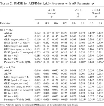
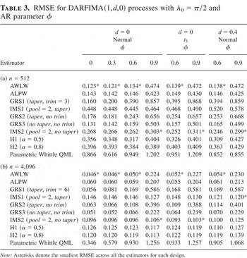
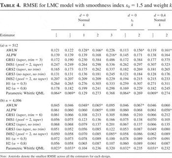
Tables 2, 3, and 4 contain the Monte Carlo RMSE results for the three models and the various estimators. Each table has a separate panel of results for n = 512 and n = 4,096. The first four rows of each panel give results for the “theoretically justified” adaptive estimators. The next rows give results for the adaptive estimators that do not (currently) have theoretical justification and for the parametric Whittle QML estimator.
RMSE for ARFIMA(1,d,0) Processes with AR Parameter φ

RMSE for DARFIMA(1,d,0) processes with λ0 = π/2 and AR parameter φ

RMSE for LMC model with smoothness index s0 = 1.5 and weight k

For brevity, we only report a subset of the parameter combinations. For example, results for φ = −0.3, −0.6, and −0.9 are not given because they are close to those for φ = 0 and 0.3. We only give selected results for d = 0.4 and no results for d = −0.4, because the value of d has only a small effect on RMSE (except for the IMS1 estimator, which exhibits some sensitivity to d). Similarly, we only give selected results for t5 innovations and we give no results for χ22 innovations, because the innovation distribution turns out to have only a small effect on RMSE.
We start by noting some general features of the results presented in the tables. First, for d = 0 the results for normal and t5 innovations are quite similar. Second, the results with normal innovations are very similar for d = 0 and d = 0.4 (with the exception of the IMS1 estimator, which is noticeably worse when d = 0.4 in all ARFIMA and DARFIMA models for n = 512). Third and not surprisingly, the performance of the AWLW and all other estimators improve substantially as n increases from 512 to 4,096 without generally affecting the qualitative ranking of the estimators.
Now, we compare the estimators. Among the four theoretically justified estimators, the AWLW and ALPW estimators perform the best in an overall sense across all three models, parameter combinations, and sample sizes. Across the 50 scenarios reported in Tables 2, 3, and 4, AWLW and ALPW have the lowest RMSE in 35 and 11 cases, respectively, among the theoretically justified estimators. For ARFIMA and DARFIMA processes with φ ≤ 0.6, the AWLW estimator uniformly outperforms the other semiparametric estimators, whereas for φ = 0.9 it is beaten by ALPW. Similar to the explanation in Remark (d) after Theorem 3.2 regarding the negative effect of large lK-values on the finite-sample bias properties of AWLW, this result for φ = 0.9 is caused by the poor approximation of ln(gj /g0) by its Taylor expansion in a neighborhood of the origin in this case. As expected, the performance of all the estimators deteriorates with increasing k in the LMC models. Compared to the ALPW estimator, the AWLW estimator has smaller RMSE when k ≤ 2; for k = 3 the comparison depends on the sample size.
Both GRS1 and IMS1 perform poorly in an absolute sense. Relative to AWLW and ALPW, GRS1 performs poorly when φ ≥ 0.3 or k ≥ 1, whereas IMS1 is outperformed for all values of k and for φ ≤ 0.6 in our models. Because of the broad-band character of the IMS1 estimator, it is not robust against discontinuous spectral densities, which is reflected in its worse performance in the DARFIMA model compared to the ARFIMA model.
Next, we consider the adaptive estimators GRS2, GRS3, and IMS2 without theoretical justification. GRS2 and GRS3 perform noticeably better than GRS1, especially when φ or k is large. Hence, trimming is found to have a negative impact. The GRS3 estimator outperforms the GRS2 estimator across all cases and all models considered. Hence, tapering also is found to have a negative impact. In an overall sense, the GRS3 estimator performs reasonably well relative to the other semiparametric estimators. However, with very few exceptions its performance is worse than that of the AWLW estimator. The IMS2 estimator outperforms the IMS1 estimator in all but two cases. In many cases the difference is substantial. Hence, again we find the effect of tapering to be negative. Compared to other semiparametric estimators, IMS2 performs best in the cases where the short-run contamination is highest, that is, φ = 0.9 or k = 3. But in most other cases it is outperformed by the AWLW, ALPW, and GRS3 estimators. It appears that the relative performance of the IMS2 estimator compared to the narrow-band AWLW, ALPW, and GRS1–3 estimators improves as the sample size increases from 512 to 4,096. The H1 and H2 estimators perform well when the sample size is 4,096 and φ or k are large. In other cases, they do not perform well relative to the AWLW, ALPW, or GRS3 estimators. In particular, they perform poorly for DARFIMA processes except when φ = 0.9. The relative strengths of the H1 and H2 estimators are similar to those of the IMS1 and IMS2. This is not surprising, because all of these estimators are broad-band FEXP estimators.
The parametric Whittle QML estimator performs as expected. For ARFIMA processes it typically has smaller RMSE than the semiparametric estimators, often substantially smaller, for example, when φ = 0.9 or n = 4,096. For DARFIMA processes, for which it is misspecified, it performs very poorly. It is substantially outperformed by all semiparametric estimators. For LMC processes, for which it is misspecified, it has lower RMSE than the semiparametric estimators for small values of k (when the LMC process is close to ARFIMA processes). But, it is outperformed for larger values of k. One surprising finding that is worth mentioning is that the parametric Whittle QML is outperformed by AWLW for certain parameter combinations in the ARFIMA model, for example, for n = 512 and φ = 0.3.
To conclude, among the four theoretically justified estimators, the new AWLW estimator seems to be the best. Of all the semiparametric estimators, the two best ones in an overall sense seem to be AWLW and ALPW. When the short-run contamination is not too large, AWLW outperforms ALPW, and the opposite is true when the short-run contamination is large. Trimming hurts the performance of the GRS1 estimator. Tapering hurts the performance of the GRS1 and IMS1 estimators. The narrow-band estimators AWLW and ALPW perform well over a broad range of parameter values but are outperformed by the broad-band estimator IMS2 when the short-run contamination is very large. The broad-band estimator IMS2 performs relatively well when the sample size is large and the short-run contamination is large. The parametric Whittle QML estimator performs very well when the model is correctly specified, moderately well when the amount of misspecification is small, and disastrously when the amount of misspecification is large.
APPENDIX: Proofs
The next lemma is needed for the proof of Lemma 3.1. It is a refined version of statements in Lemma 2 of Andrews and Guggenberger (2003).
LEMMA A.1. Suppose Assumption AG4 holds. Then, for Jm defined in (3.11),

Proof of Lemma A.1. For the proof we need the following approximations:

These approximations follow from straightforward calculations using the following version of Euler's summation formula (see, e.g., Walter, 1992, p. 349). For f ∈ C3([1,m]), we have

where

is the pth Bernoulli polynomial, and Bj in this lemma denotes the jth Bernoulli number. It can be shown that E2(m) = 6−1 and for all real numbers x, |E3(x)| < 20−1. For part (i) of Lemma A.1 then note that

where the second equality follows from (a) and (b). Part (i) then follows. For part (ii), note that using (a), (c), and (d), we have

Proof of Lemma 3.1.
Part (i). The log-periodogram can be written as

where Rj := ln gj − ln g0 and εj := ln(Ij /fj) + C; see (2.2). Define the m-vectors R(m) := (R1,…, Rm)′ and ε(m) := (ε1,…, εm)′. Then

By Lemma 2(a) and (f) in Andrews and Guggenberger (2003),

Regarding Jm−1 X*(m)′R(m), first note that under Assumption AG2, a Taylor expansion of ln gj about λ = 0 as in Andrews and Guggenberger (3.3) yields

where bk := (dk/dλk)ln g(λ)|λ=0, Remj, defined implicitly as the difference between Rj and the sum on the right-hand side, satisfies max1≤j≤m|Remj /λjq| = O(1) for q defined in (2.7) and max1≤j≤m|Remj /λjq| = o(1) if s = 2 + 2r. Combining this with Lemma A.1(ii) and using Andrews and Guggenberger (7.16) yields

where the second equation uses Lemma A.1(i). The O(mq/nq) term in (A.4) is o(mq/nq) if s = 2 + 2r. Note that O((m2k−1/n2k)ln2 m) is dominated by O(m−1 ln3 m) from (A.2). Combining (A.1), (A.2), and (A.4) yields the desired result.
Part (ii). Let

. Without loss of generality, we assume that li ≤ lj. Because (X*′X*)−1 = 4−1m−1(1 + o(1)), (A.1) implies that

where Xki* := Xk*(mi). We decompose the double sum in the formula for Cov into

.
By Lemma 2(k) in Andrews and Guggenberger (2003), max1≤k≤mv|Xkv*| = O(ln mi) for v = i and j. Similar calculations to the ones in Lemma A.1(i) yield

. Thus, the proof of Theorem 1 in Hurvich et al. (1998) where they calculate the variance of the GPH estimator (p. 25) can be modified along the same lines as done in the proof of Theorem 1(b) in Andrews and Guggenberger (p. 702) to prove that the first part of the double sum equals

. It is easily shown that the contribution of the second part is in o(mi) and thus negligible and thus Cov = (4π2mi /(96mi mj))(1 + o(1)) = (π2/(24lj m))(1 + o(1)). █
Proof of Theorem 3.3. The proof is analogous to the proof of Theorem 2 in Andrews and Guggenberger (2003). The latter proof in turn relies on the proof of Theorem 2 in Hurvich et al. (1998) and the proof of (5.14) in Robinson (1995b). Note that by the definition of

and Lemma A.1(i)

It follows from equation (A.4), the fact that the weights satisfy (3.2)–(3.4), and the rate condition m2.5+2r/n2+2r → χ that for the first summand we get

Ignoring the op(1) term, the second summand can be written as

, where

and 1(·) is the indicator function. The same proof as in Andrews and Guggenberger (see p. 705, following eqn. (7.24)) can be used to show that

We just have to verify conditions (i)–(iii) of the asymptotic normality result in Andrews and Guggenberger (7.28), which then yields the desired result. For (i) note that by Lemma 2(k) in Andrews and Guggenberger we have max1≤j≤mK|Xji*| = O(ln m) and thus max1≤j≤mK|aj| = O(ln m). For (ii),

for li < lk implies that

. Finally, for (iii) note that from Andrews and Guggenberger (7.30) we have

for all p ≥ 1. This implies

for all p ≥ 1. █
To prove Theorem 3.4 and establish the asymptotic properties of

, we first investigate those of

. For some d+ between

and d we have

If

, then applying Lemma 2(b) and (d) of Andrews and Sun (2004) for the case r = 0 (in which case their θ and θ0 are not present) yields Jm−1Hm(d+) − 1 = op(1). As a consequence of (A.5),

To show that

, by an induction argument it suffices to show that

and that

. The former is assumed through

, and the latter is proved now. The term ((1/m)Jm)−1 is Op(1) by Lemma A.1(i), and so we are left with the term

. Some algebra (see Andrews and Sun, 2004, eqn. (4.2)) gives


The second equality in (A.7) uses the fact that E2πIεj = 1. For notational convenience, we write Tj = Tj(m), j = 1,…,4. In the proof of their Lemma 2(e), Andrews and Sun show that T1 = T2 = op(1) as 1/m + m/n → 0. The asymptotic properties of T3, T4, and

are established in the next lemma. These properties combined with T1 = T2 = op(1) imply that

.
LEMMA A.2. Suppose Assumptions AS1–AS4 hold.
(i) Let T3i := T3(mi). Then

(ii) For s = 1,…, r + 1 let

where the ij (j = 1,…, k) are positive integers. Then

where q is defined in (2.7) and O(m0.5+q/nq) can be replaced by o(m0.5+q/nq) if s = 2 + 2r.
(iii) For real numbers B2j (j = 1,…, r) defined in (A.15), which follows, we have

Note that

depends on m.
Proof of Lemma A.2.
Part (i). Using the Cramer–Wold device, we need to show that for ρ = (ρ1,…, ρK)′ we have

. Note that

Robinson (1995a, from line 11 on p. 1644 to line −6 on p. 1647) proves that

where

. Inspection of his proof reveals that (A.12) continues to hold with νp replaced by νp* if the following properties of the νp* sequence hold: (i) νp* = O(log mK) and (ii)

. Property (i) holds trivially, and (ii) holds because

So

Therefore part (i) follows upon showing that

. But

equals

for

where the second to last equality follows from Lemma 2(a) in Andrews and Guggenberger (2003). Thus, (A.9) follows.
Part (ii). Using (A.3), ln(fj /φj) = Rj, and applying “exp” on both sides implies that for A2k defined in (A.10), we have

Therefore,

where for the second equation we used equation (7.16) in Andrews and Guggenberger and the O can be replaced by o if s = 2 + 2r. Using Lemma A.1(ii), we thus get the desired result:

Part (iii). We show that for certain constants

defined in (A.17), which follows, we have

It is tedious but straightforward to show that this implies the desired result (A.11) for

where M = (Mi,j) is a lower triangular r × r matrix with the number 1 on the main diagonal and Mi,j := C2(i−j) for i > j. To prove (A.14), write

where

We claim that

for i = 1,2, and 3. In fact, equation (A.21) of Andrews and Sun (2004) (with their gj playing the role of our φj, their φ = 2, and k = m) states that

, where for the last equality we use Assumption AS4. Equation (A.23) of Andrews and Sun states that E(Ij /fj) = 1 + O(j−1 ln j) uniformly over j = 1,…, m. Therefore

. Equation (A.13) of Andrews and Sun states that

. Finally (A.13) implies that

where the second equality uses (d) in the proof of Lemma A.1. This proves (A.14) with

█
Proof of Theorem 3.4. It follows from equation (A.6),

, and Lemma A.1(i) that

Using (A.7), T1 = T2 = op(1), and Lemma A.2(ii) and (iii), it follows that the O((ln2 mi)/mi) term in (A.18) can be ignored (Assumption AS4 implies that O((ln2 m/m)(m2.5/n2)) = o(1), and thus the statement follows by noting that m2.5/n2 is the highest order term of T4 that hits O(ln2 m/m); for similar reasons we can ignore the O(ln m/m) terms in T4 in equation (A.20)) and thus

Lemma A.2(i) implies that

. Using Lemma A.2(ii) and (iii), (3.3), (3.4), and AS4, we have, up to op(1) terms, for B0 := 1

Setting

and combining the preceding statements gives

that is,

To prove Theorem 4.3 we need the following lemma, to be proved subsequently. Unless otherwise stated, from now on C is a generic constant that may be different across different lines.
LEMMA A.3. Suppose the assumptions of Theorem 4.3 hold.
(i) For any constant C > 0, we have

(ii) If s0 < ∞, then for any constant C > 0,

Proof of Theorem 4.3.
Part (i). Set s := min(s0,s*) and recall that h = 1/ln n. We first bound

. We have

. By the definition of

, if

, there exists

such that

In consequence, for all

with τ + h < s,

where κ := ψ2(cr(s*)*/4)1/2/2. Note that we used that cr* is an increasing function in r. The last inequality holds because there are at most (s* − s*)(ln n) elements

for which τ′ ≤ τ. It now follows from Lemma A.3(i) that

If s0 = ∞ (and thus s0 ≥ s*), then (A.22) clearly implies the result in part (i). Therefore from now on we can assume s0 < s*. We now prove that

. Assume without loss of generality that

. By the definition of

,

where the last two equalities use both parts of Lemma A.3. In the preceding proof, we implicitly assume that

. If this is not the case, we can bound

by

where

. The rest of the proof goes through with obvious changes.
Combining (A.22) and (A.23), we get

as desired, completing the proof of Theorem 4.3(i).
Part (ii). Let

; then

. Using the definition of

and Lemma A.3(i), we have

uniformly as C → ∞, where the last equality holds because

To prove Lemma A.3, we introduce some notation and state one more lemma. Let

be defined as the corresponding quantities

(from (A.8)) with m replaced by mi,τ = li mτ. Unless otherwise stated, from now on “uniformly” stands for “uniformly over τ ∈ [s*,min(s0,s*)].”
LEMMA A.4. Set

. Then, under Assumptions AS1, AG2(b), and AS3, and for a = 1, 2, and 3 we have uniformly

Proof of Lemma A.4.
Part (i). Inspection of the proof of Lemma 7 of Andrews and Sun (2004, p. 609) shows that if mi,τ = O(nΔ) for some Δ < 1, then uniformly

Part (i) holds because mi,τ = O(n2τ/(2τ+1)) satisfies the required rate condition.
Part (ii). Recall from (A.16) that

To prove part (ii), it suffices to prove that uniformly for a = 1,2,3


The proofs of (A.26) and (A.27) use the following result: if a sequence hj(τ) = hj(mτ), j = 1,…, mτ uniformly satisfies

then

To prove (A.28), note that by Theorem 5.2.4 of Brillinger (1975, p. 125) and Andrews and Sun (2004, p. 604), Var(Iεj) = O(1) and Cov(Iεi,Iεj) = O(n−1) uniformly over i,j = 1,…, n with i ≠ j. Thus, as desired, (A.28) equals

We now proceed to establish (A.26). For a = 1, we use a proof similar to the Andrews and Sun (2004) proof of their (A.21) on p. 603. Recall that

Let [ell ] := (mi,τ)1/3(ln mi,τ)2/3 and

Using E|Ijφj−1| ≤ C, for j = 1,…,[ell ], proved in Robinson (1995a, eqn. (3.16)), we have

We decompose the remaining summands in

into

We can uniformly bound EA112 by

where the equality holds by the same proof as in Robinson (1995a, pp. 1648–1651) for the quantity given in the third equation on his p. 1648. The only difference is that the factor fj /φj does not appear in Robinson (1995a). It can be shown that this factor has no impact on the proof because fj /φj = 1 + o(1) uniformly over j = 1,…,.mi,τ. For A12, we have

uniformly, where φ = min(τ,2) and we have used Theorem 5.2.4 of Brillinger (1975, p. 125) again. Combining (A.29)–(A.32) and using 2r(τ) < τ gives

For a = 2, (A.26) holds because uniformly

. For a = 3, by Markov's inequality

uniformly, where the second inequality follows from (A.28) by setting hj(τ) = 1 and the last equality holds because 4r(τ) − 2τ < 0. This proves (A.26). To prove (A.27), we only need to show that

, because

is nonrandom. In the proof of part (iii) of Lemma A.2, we have shown that

, and it is easy to see that the o(mi,τ2r(τ)/n2r(τ)) term is actually O((mi,τ)τ/nτ). In view of 2r(τ) < τ, we get

as required.
Part (iii). The result holds for a = 2 because

uniformly, where we have used EIj /fj − 1 = O(j−1 ln j) and Xj* = O(ln mi,τ) uniformly over j = 1,…, mi,τ.
Part (iii) holds for a = 3 because ET3,iτ2 = O(1) uniformly, using (A.28) with hj = Xj* and then

Finally, for a = 1, we can prove part (iii) using a proof similar to that of (A.26) for a = 1. Details are omitted. █
Proof of Lemma A.3. We prove only the case for the one-step estimator. The extension to the general k-step estimator is straightforward. Recall that mi,τ = li mτ.
Part (i). In the proof of Theorem 3.4, we have shown that, for some di,τ+ between

,

where {wi,τ}i=1K are the weights when r = r(τ),

and mi,τ1/2(di,τ+ − d) = Op(1).
We now consider each of the two terms in (A.33). It follows from Lemma A.1(i) and Lemma A.4(i) that uniformly

and thus

uniformly. Using the preceding inequality, we have uniformly

where the last equality follows from Theorem 3.2. The uniformity holds because the

is uniformly bounded for τ in a finite interval.
Next, we show that for some C > 0,

As in the proof of Lemma A.2, we write

Let

denote the event

. It follows from Lemma A.1(i) and Lemma A.4(ii) that

uniformly if C is large enough, where

is the complement of

. We can therefore focus on the event

.

and the last summand is uniformly O(ζ−2(n)) by Lemma A.4(iii). To bound the probability in (A.38), note that when

is true

where the small order term is o((mi,τ /n)2r(τ)) instead of op((mi,τ /n)2r(τ)) and

where φ = min(τ,2) and

Using (A.39) and (A.40) and letting

, we have

uniformly, which implies that the probability in (A.38) is O(ζ−2(n)). Combining this with (A.33) and (A.35) gives the desired result.
Part (ii). For notational simplicity, set τ0 := s0 + 8s0 h ln ln n so that

The last equality holds because

As in the proof of part (i), we write

where for some di,τ0+ between

,

We now consider em,τ0, the second term in (A.42). Set

It follows from Theorem 3.2 that

Hence

As a consequence, we can now focus on the case di,τ0+ ∈ Dmi,τ0. To obtain a bound for P(|em,τ0| > Cζ−1(n)V(τ0)), we use the following result:

which is slightly stronger than (A.25) with τ = τ0. Inspection of the proof of Lemma 7 of Andrews and Sun (2004, p. 609) shows that the preceding result holds. Using (A.44), we have

Next, we consider the first term in (A.42). Using a proof similar to (A.36), we get for a = 1,2,3

Let

Then it follows from (A.41), (A.42), (A.45), and (A.46) that

Let

denote the event

. A proof similar to the one for Lemma A.4(ii) shows that

It follows from the preceding equation and Lemma A.1(i) that

. As before, we now focus on the event

, in which case,

implying that the dominating term in

is at least

for some nonzero constant C.
We now prove that

can be bounded from below by C ln2 n for some constant C > 0. We know that

and therefore by the definition of Xj* it is enough to bound |B| from below by C ln2 n, where

. Set m0 := mτ0 /e. Then −ln j + ln mτ0 − 1 ≤ 0 iff j ≥ mτ0. So when RT(λ) > 0 for all λ ∈ U

using (4.4) where C > 0 is a constant. Similarly, when RT(λ) < 0 for all λ ∈ U,

Therefore, under (4.4)

where C* is a positive constant. As a result, up to lower order terms

However, because

as 8s0 /(2s0 + 1)2 is a decreasing function of s0 when s0 ≥ 1, we have

and thus

when n is large enough. Combining this with (A.47) leads to the stated result. █