2.1. Planning-level abstraction of the cable-driven snake-like robot

As shown in Figure 1, the CDSR is mainly composed of three parts: a rear-mounted drive device, a linear feeding unit, and a connecting arm body.

Table I.

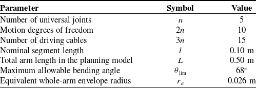
Main structural parameters of the CDSR.

Table I. Long description

A table with three columns and eight rows. The columns are labeled Parameter, Symbol, and Value. The rows list various parameters related to a snake-like arm, their corresponding symbols, and values. Row 1: Parameter, Number of universal joints; Symbol, n; Value, 5. Row 2: Parameter, Motion degrees of freedom; Symbol, 2n; Value, 10. Row 3: Parameter, Number of driving cables; Symbol, 3n; Value, 15. Row 4: Parameter, Nominal segment length; Symbol, l; Value, 0.10 meters. Row 5: Parameter, Total arm length in the planning model; Symbol, L; Value, 0.50 meters. Row 6: Parameter, Maximum allowable bending angle; Symbol, theta_lim; Value, 68 degrees. Row 7: Parameter, Equivalent whole-arm envelope radius; Symbol, r_a; Value, 0.026 meters.

Figure 1.

Three-dimensional structural model of the cable-driven snake-like robot (CDSR).

Rear-mounted drive device: This device is centrally arranged inside the robot base. Its main transmission components include the stepper motor, coupling, pulley assembly, and linear motion module. During operation, the rotational motion generated by the stepper motor is transmitted to the pulley assembly through the coupling and is further converted into the axial linear motion of the linear motion module. This linear motion is then converted into cable-length variation, thereby realizing the traction control of multiple driving cables. The rear-mounted drive layout effectively reduces the weight and rotational inertia of the distal connecting arm body, which improves the dynamic response and motion flexibility of the snake-like robot in narrow confined spaces.

Linear feeding unit: The linear feeding unit is arranged at the bottom of the snake-like robot and is used to support the rear-mounted drive base while providing overall axial feeding motion. In practical operation, the linear feeding unit drives the arm to advance or retract along the main axial direction, allowing the snake-like robot to gradually enter the utility tunnel and providing the basic translational motion for subsequent universal-joint posture adjustment and distal inspection.

Connecting arm body: The connecting arm body consists of five universal joints connected in series, with adjacent joints linked by rigid connecting sections. After being drawn out from the rear-mounted linear motion module, the driving cables pass successively through the guiding holes near each universal joint and are finally fixed at the corresponding distal positions. By adjusting the length variations of different driving cables, the spatial postures of the universal joints can be changed, thereby realizing whole-arm bending, steering, and configuration adjustment of the snake-like robot.

By controlling the stepper motor to drive the axial displacement of the linear motion module, the rear linear motion is converted into cable-length variation. Under the coordinated traction of multiple cables, the spatial postures of the five distal universal joints can be constrained and controlled. To clarify the overall scale and motion capability of the CDSR, the main structural parameters are summarized in Table I.

In the path-planning stage, it is unnecessary to reconstruct every detail of the continuous deformation. The emphasis is on whether a sequence of planning-level acceptable configurations can be generated stably. Therefore, this paper adopts a planning-level abstraction that combines a discrete backbone with the PCC assumption. As shown in Figure 2, the centerline of the CDSR is discretized into ordered backbone points, and the nominal segment length $\mathrm{l}$ between adjacent backbone points and the planning-level equivalent envelope radius ${r}_{{a}}$ are used to describe the geometric occupancy of the whole arm.

Figure 2.

Planning-level geometric abstraction and equivalent envelope schematic.

Let $\mathcal{W}\subset {R}^{3}$ denote the three-dimensional workspace, and let $\mathcal{O}\subset \mathcal{W}$ denote the obstacle region. The free space is defined as

(1) \begin{equation} \mathcal{W}_{f}=\mathcal{W}\setminus \overline{\mathcal{O}}. \end{equation}

where $\overline{\mathcal{O}}$ denotes the closure of the obstacle region, which is introduced to avoid ambiguity caused by contact between the path and obstacle boundaries.

The centerline of the snake-like robot is discretized into ${N}$ ordered backbone points and denoted as

(2) \begin{equation} P=\left\{p_{0},p_{1},\ldots ,p_{N-1}\right\}\!,\quad \quad l=\frac{L}{N-1}. \end{equation}

where $p_{0}$ denotes the head-guidance point, $p_{N-1}$ denotes the backbone point close to the base, $L$ denotes the total length of the arm, and $l$ denotes the nominal segment length between adjacent backbone points. Through this discretization, the continuum manipulator is transformed at the planning level into a finite-dimensional state vector, and subsequent updating, collision checking, and constraint evaluation can be performed on the same set of variables.

Checking only whether the centerline is collision-free cannot guarantee safe passage of the whole arm. In narrow gaps and bends, even when the centerline appears to have sufficient clearance, the outer contour of the arm may still contact obstacles or the utility-tunnel boundary. Therefore, the equivalent whole-arm envelope set is further defined as

(3) \begin{equation} A(P)=\underset{i=0}{\bigcup ^{N-2}}\left\{x\in \mathbb{R}^{3}\mid d_{\mathrm{seg}}(x,[p_{i},p_{i+1}])\leq r_{a}\right\}\!. \end{equation}

where $d_{\mathrm{seg}}(x,[p_{i},p_{i+1}])$ denotes the shortest distance from point ${x}$ to the line segment $[p_{i},p_{i+1}]$ , and $r_{a}$ is the planning-level equivalent envelope radius of the arm. The equivalent envelope shown in Figure 2 corresponds to the whole-arm occupied region defined by Eq. (3). This set approximates the outer contour of the real mechanism using dilated line segments so that collision-free checking is performed on the whole-arm envelope rather than only on the discrete backbone centerline.

2.2. Definition of discrete curvature and tension risk

The traversability of the whole arm is jointly constrained by its geometric shape and cable-driven actuation capability. This subsection first computes the curvature from the discrete centerline and then maps the curvature to cable-length variation and a tension-risk proxy. As shown in Figure 3, the discrete curvature is characterized by local bending units formed by adjacent backbone segments, where the turning angle $\theta _{i}$ between adjacent segments is used to compute the equivalent curvature $\kappa _{i}$ of the $i$ -th discrete bending unit. This sequence is consistent with the actual mechanical relationship: backbone bending induces cable-length variation, and cable-length variation reflects whether a candidate configuration approaches the actuation boundary.

Figure 3.

Geometric representation of discrete curvature and local bending units.

Assumption 1: At the planning level, each bending unit satisfies a piecewise constant-curvature approximation, and a neutral layer with invariant length exists within the unit. The radial offset of each driving cable relative to the neutral layer is a constant $r_{t}$ . The cable can sustain tension but not compression. The unit bending satisfies $0\leq r_{t}\kappa _{j}\lt 1$ , so that the cable-hole trajectory radius remains positive. This assumption is used to establish a monotonic mapping from geometric quantities to actuation risk at the planning level. High-fidelity execution-level dynamics are beyond the scope of this paper. This assumption corresponds to the constant-curvature and cable-offset modeling commonly used for cable-driven continuum robots [Reference Webster and Jones3, Reference Rucker and Webster4, Reference Camarillo, Milne, Carlson, Zinn and Salisbury31], and only the associated monotonic geometric relationship is used at the planning level.

Let $l$ denote the nominal segment length between adjacent backbone points. The unit tangent vector of the $i$ -th segment is given by

(4) \begin{equation} \tau _{i}=\frac{p_{i}-p_{i-1}}{\parallel p_{i}-p_{i-1}\parallel },\quad \quad i=1,2,\ldots ,N-1. \end{equation}

where $\tau _{i}$ denotes the local direction of the $i$ -th segment. Since the subsequent FTL update strictly preserves the discrete segment length, $\parallel p_{i}-p_{i-1}\parallel$ and ${l}$ have the same geometric scale at the planning level. The actual denominator is retained to suppress numerical accumulation errors during iteration.

The turning angle between two adjacent segments is defined as

(5) \begin{equation} \sigma _{i}=\tau _{i}\top \tau _{i+1},\bar{\sigma }_{i}=\min \{1,\max \{-1,\sigma _{i}\}\}. \end{equation}

(6) \begin{equation} \theta _{i}=\arccos (\overline{\sigma }_{i}). \end{equation}

where $i=1,2,\ldots ,N-2$ . This index range corresponds to the discrete bending units formed by three adjacent backbone points.

In the equation, $\theta _{i}$ is the included angle between adjacent backbone segments, and $\overline{\sigma }_{i}$ is used to restrict the inner-product result to [−1,1], thereby avoiding out-of-range values in the inverse trigonometric calculation. If the two adjacent segments are regarded as polyline segments of equal length $l$ , the chord-length relation of the circumcircle satisfies $2\sin (\theta _{i}/2)=\kappa _{i}l$ , from which the discrete curvature expression adopted at the planning level can be obtained.

(7) \begin{equation} \kappa _{i}=\frac{2\sin \left(\theta _{i}/2\right)}{l}\approx \frac{\theta _{i}}{l},\quad \quad i=1,2,\ldots ,N-2. \end{equation}

where $\kappa _{i}$ denotes the equivalent curvature of the $i$ -th discrete bending unit. The local bending unit shown in Figure 3 intuitively corresponds to the curvature calculation process in Eqs. (5)–(7): the turning angle $\theta _{i}$ is first obtained from the directions of adjacent segments, and the equivalent curvature $\kappa _{i}$ is then determined from $\theta _{i}$ and the nominal segment length $l$ . When the angle $\theta _{i}$ between adjacent segments is small, $\frac{2\sin (\theta _{i}/2)}{l}$ can be approximated by $\frac{\theta _{i}}{l}$ . This approximation means that the local chord length $l$ formed by adjacent backbone segments is used to approximate the arc length at that location, and the turning-angle variation between adjacent tangent vectors is used to describe the local bending degree. In this paper, five bending units are adopted at the planning level, with a unit length of 0.10 m and a single-step advancement of approximately 0.03 m. At this discretization scale, the above expression can be used for curvature evaluation and screening of candidate configurations. The refined continuum deformation at the execution level still needs to be further solved using a high-fidelity model.

According to the planning-level discretization scale and a conservative curvature margin, the maximum allowable turning angle between adjacent discrete backbone segments is set to 68°. From the discrete-curvature approximation $\kappa _{i}\approx \frac{\theta _{i}}{l}$ , when the nominal unit length is $l=0.10\,\mathrm{m}$ , 68° (1.1868 rad) corresponds to an equivalent curvature upper bound of approximately 11.18 $\mathrm{m}^{-1}$ . This value is used for candidate-configuration screening and the acceptable-success criterion. Its role is to suppress local over-bending and to retain a safety margin for whole-arm envelope sweeping and cable-tension distribution, rather than to represent the absolute physical limit of the mechanism at the execution level. In subsequent prototype experiments, this threshold can be further calibrated according to the measured curvature limit.

The maximum bending-angle constraint can limit local overbending, but it cannot by itself characterize the smoothness of the whole-arm shape. If curvature changes too rapidly between adjacent units, the configuration may still exhibit sharp corners, oscillations, or unstable jumps even when the peak value does not exceed the limit. To constrain both the bending magnitude and the curvature variation rate, discrete bending energy and curvature-gradient energy are introduced in this paper. Related reviews also point out that planning for cable-driven continuum robots should consider not only centerline reachability but also bending constraints and actuation feasibility [Reference Dupont, Simaan, Choset and Rucker6, Reference Bai, Lee, Yang, Shen, Qian, Zhang, Zhou, Fang, Zheng, Yang, Huang and Yu7, Reference Rao, Peyron, Lilge and Burgner-Kahrs32] .

(8) \begin{equation} J_{\kappa }(P)=\mathop{\sum }\limits_{i=1}^{N-2}{\kappa }_{i}^{2}l. \end{equation}

(9) \begin{equation} J_{\Delta \kappa }(P)=\frac{1}{l}\mathop{\sum }\limits_{i=1}^{N-3}(\kappa _{i+1}-\kappa _{i})^{2}. \end{equation}

where $J_{\kappa }(P)$ is the discrete approximation of the continuous elastic-rod bending energy $\int\! \kappa ^{2}ds$ , which mainly limits the overall bending magnitude of the whole arm. $J_{\Delta \kappa }(P)$ is the discrete form of the curvature-gradient energy $\int \!\left(\frac{\partial \kappa }{\partial s}\right)^{2}ds$ , which suppresses abrupt changes between adjacent bending units. The former controls bending magnitude, while the latter controls the curvature variation rate, and the two terms are not interchangeable in candidate-configuration evaluation.

Figure 4.

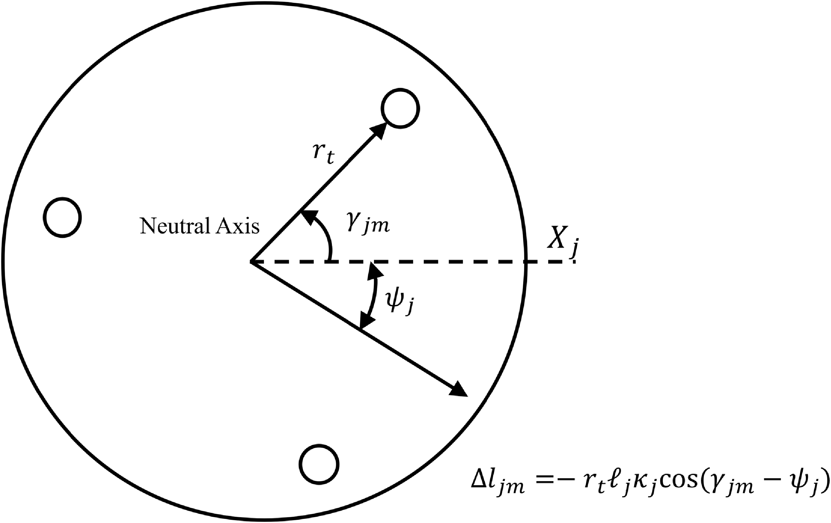
Cross-sectional cable layout and cable-length variation mapping.

As shown in Figure 4, the cross-sectional cable-hole layout determines the projected offset of each driving cable relative to the bending plane. Therefore, geometric bending can be further mapped to cable-length variation and a tension-risk proxy. The geometric bending is then related to the cable-driven actuation boundary. Let $\ell_{j}$ denote the neutral-layer arc length of the $j$ -th bending unit, $\kappa _{j}\geq 0$ denote the curvature magnitude, and $\psi _{j}$ denote the bending-plane angle. In this paper, the parameterization convention is adopted in which the curvature magnitude is given by $\kappa _{j}$ , whereas the bending direction is given by $\psi _{j}$ . Therefore, $R_{j}=1/\kappa _{j}$ represents the geometric curvature radius, while the directional information is separately characterized by $\psi _{j}$ . Let $\gamma _{jm}$ denote the circumferential angle of the $m$ -th driving cable on the cross section, and let $r_{t}$ denote the radial distance from the cross-sectional center to the cable hole. The projected offset of this cable hole relative to the bending plane is $r_{t}\cos (\gamma _{jm}-\psi _{j})$ , and its trajectory radius is approximated as $1/\kappa _{j}-r_{t}\cos (\gamma _{jm}-\psi _{j})$ . Therefore, the arc length of this cable in the unit is given by

(10) \begin{equation} R_{j}=\frac{1}{\kappa _{j}},{\quad}{\quad}\alpha _{j}=\kappa _{j}\ell_{j}. \end{equation}

where $R_{j}$ is the curvature radius of the neutral layer, and $\alpha _{j}$ is the central bending angle of the unit. From the neutral-layer arc-length relation $\ell_{j}=R_{j}\alpha _{j}$ , the arc length of any offset cable can be expressed as the product of the local trajectory radius and the same central angle. Therefore, the trajectory radius of the $m$ -th cable in this unit is given by

(11) \begin{equation} R_{jm}=R_{j}-r_{t}\cos (\gamma _{jm}-\psi _{j}). \end{equation}

(12) \begin{align} {l}_{{jm}}={\unicode{x03B1}} _{{j}}{R}_{{jm}}& ={\unicode{x03BA}} _{{j}}\ell_{{j}}\left(\frac{1}{{\unicode{x03BA}} _{{j}}}-{r}_{{t}}\cos ({\unicode{x03B3}} _{{jm}}-{\unicode{x03C8}} _{{j}})\right), \nonumber\\ {l}_{{jm}} &=(1-{r}_{{t}}{\unicode{x03BA}} _{{j}}\cos ({\unicode{x03B3}} _{{jm}}-{\unicode{x03C8}} _{{j}}))\ell_{{j}}\end{align}

Subtracting the neutral-layer arc length $\ell_{j}$ from it gives the cable-length variation

(13) \begin{equation} \Delta l_{jm}=l_{jm}-\ell_{j}=-r_{t}\ell_{j}\kappa _{j}\cos (\gamma _{jm}-\psi _{j}). \end{equation}

In the straight-line limit where $\kappa _{j}=0$ , $l_{jm}=\ell_{j}$ and $\Delta l_{jm}=0$ can be taken. Therefore, $1/\kappa _{j}$ in the formulation is only an intermediate geometric expression and does not imply a real singularity in the straight-line case. It should be further noted that $\Delta l_{jm}$ is defined in this paper as the change in the geometric arc length of the cable relative to the neutral-layer arc length. If the more common convention in some studies, in which positive actuator input denotes cable retraction, is adopted, the corresponding variable should be written as $-\Delta l_{jm}$ . Therefore, the difference from constant-curvature cable-driven formulations mainly arises from the sign convention, while the underlying geometric relationship remains consistent. This geometric mapping is consistent with the inverse-kinematic expression for cable-actuated constant-curvature sections proposed by Jones and Walker and is also compatible with the unified formulations in subsequent PCC/TDCR modeling reviews [Reference Jones and Walker2, Reference Webster and Jones3, Reference Rao, Peyron, Lilge and Burgner-Kahrs32].

The neutral layer, cable-hole circumferential angle, and radial offset shown in Figure 4 jointly determine the sign and magnitude of $\Delta l_{jm}$ . Therefore, the tension-risk proxy is related not only to the curvature magnitude but also to the bending-plane direction and the cable-hole layout. Here, $\Delta l_{jm}\lt 0$ indicates that the cable is shortened relative to the neutral layer, whereas $\Delta l_{jm}\gt 0$ indicates that it is lengthened. The cosine term in the formulation represents the coupling between the bending-plane direction and the cable-hole circumferential orientation; therefore, the tension-risk proxy is jointly determined by the curvature, bending plane, and cable-hole layout.

To map $\Delta l_{jm}$ to a risk quantity that can be compared at the planning level, a linear equivalent axial constitutive relation is further adopted as

(14) \begin{equation} {T}_{jm}^{\mathrm{lin}}=T_{\mathrm{pre},\,jm}-k_{t}\Delta l_{jm}. \end{equation}

where ${T}_{jm}^{\rm lin}$ denotes the linear axial-tension prediction before slack-cable states are considered, $T_{\mathrm{pre},\,jm}$ is the pretension, and $k_{t}$ is the equivalent axial stiffness. A real cable can sustain only tension, and the compressive component calculated by the linear model does not correspond to an actual negative tension. Based on this observation, only the positive part of the predicted tension is retained at the planning level and used as a proxy indicating whether a candidate configuration approaches the actuation-risk boundary.

(15) \begin{equation} {T}_{jm}^{\text{risk}}=\max (0,T_{\mathrm{pre},\,jm}-k_{t}\Delta l_{jm}). \end{equation}

where $\Delta l_{jm}\lt 0$ indicates that the cable segment is retracted and the linear tension prediction increases, whereas $\Delta l_{jm}\gt 0$ indicates that the cable segment is lengthened and the negative-tension component is truncated to zero. ${T}_{jm}^{\rm risk}$ is not equivalent to the real tension at the execution level but is a conservative risk indicator obtained under ideal frictionless and linear-elastic assumptions. In this paper, this indicator is used only at the planning stage to identify and eliminate high-risk candidate configurations, rather than to replace tension solving that accounts for friction, transmission attenuation, and material nonlinearity. The cable-offset, pretension, and equivalent axial-stiffness parameters used in the simulations are specified within the planning-level normalized model. These parameters provide a consistent relative scale for evaluating the tension-risk proxy among candidate configurations and are not obtained from hardware-level tension calibration.

2.3. Whole-arm safety clearance and admissible configurations

After the envelope, curvature, and tension-risk proxy have been defined, the planning-level admissible configuration set can be further defined as follows. First, the shortest distance from an arbitrary point to the free-space boundary is defined as

(16) \begin{equation} d_{\partial {\mathcal{W}_{f}}}(x)=\text{dist}(x,\partial \mathcal{W}_{f}). \end{equation}

By further subtracting the equivalent envelope radius $r_{a}$ , the effective clearance in terms of the whole-arm envelope is obtained as

(17) \begin{equation} c(x)=d_{\partial {\mathcal{W}_{f}}}(x)-r_{a}. \end{equation}

where $c(x)\geq 0$ indicates that the local envelope sphere centered at $x$ with radius $r_{a}$ is still entirely contained in the free space, and therefore no obstacle intrusion occurs at the corresponding position. To prevent the planner from operating only on the binary condition of whether actual collision occurs, a safety-clearance penalty term is also defined in this paper as

(18) \begin{equation} J_{\text{coll}}(P)=\mathop{\sum }\limits_{i=0}^{N-1}\left[\max \left(0,d_{\text{safe}}-c\,(\ \!\!\ p_{i})\right)\right]^{2}\!. \end{equation}

where $d_{\rm safe}$ is the safety-clearance threshold. This term penalizes configurations approaching obstacle boundaries before actual collision occurs; therefore, it can both characterize the admissibility boundary and participate in subsequent soft-cost ranking.

Three configuration-level aggregate quantities are further defined as

(19) \begin{equation} \kappa _{\max }(P)=\max _{i}\kappa _{i}(P),{\quad}{\quad}{T}_{\max }^{\text{risk}}(P)=\max _{j,m}{T}_{jm}^{\text{risk}}(P),{\quad}{\quad}c_{\min }(P)=\min _{i}c\left(p_{i}\right)\!. \end{equation}

The planning-level admissible configuration set is then written as

(20) \begin{equation} \mathcal{P}_{\mathrm{ad}}=\left\{P\mid c_{\min }(P)\geq 0,\,\kappa _{\max }(P)\leq \kappa _{\lim },\,{T}_{\max }^{\text{risk}}(P)\leq T_{\max }\right\}\!. \end{equation}

The admissible configuration set in Eq. (20) is defined by whole-arm envelope nonintrusion, the maximum-curvature bound, and the tension-risk upper bound. A candidate violating any of these conditions is rejected directly. The safety-clearance penalty defined in Eq. (18) and the curvature-gradient term defined in Eq. (9) are not additional hard constraints; instead, they are incorporated into the evaluation function in Eq. (70) to rank candidates that have already passed the hard-constraint screening. Consequently, a feasible candidate with a smaller clearance margin or a larger curvature variation receives a higher soft cost. This two-stage construction clearly distinguishes configuration admissibility from preference-based ranking within the admissible set.

2.4. Planning objective on the configuration manifold

Let $x_{g}$ denote the target point, $P^{k}$ denote the configuration at the $k$ -th step, and ${p}_{0}^{k}$ denote the head position. The planning objective in this paper can be written as

(21) \begin{equation} \min _{\{P^{k}{\}}_{k=1}^{K}}\mathop{\sum }\limits_{k=0}^{K-1}M(P^{k+1}), \end{equation}

subject to

(22) \begin{equation} \parallel {p}_{0}^{K}-x_{g}\parallel \leq \varepsilon _{g},{\quad}{\quad}P^{k}\in \mathcal{P}_{\mathrm{ad}},\quad k=1,2,\ldots ,K. \end{equation}

where $K$ denotes the upper limit of planning steps, $\varepsilon _{g}$ denotes the target-neighborhood radius, $\mathcal{P}_{\rm ad}$ denotes the admissible configuration set defined in Section 2.3, and $M(P^{k+1})$ denotes the single-step candidate-configuration evaluation function. The problem simultaneously enforces target arrival, configuration admissibility, and single-step cost minimization.

3.1. Variational derivation of the harmonic potential field

The admissible configuration manifold defines which configurations can be generated, but it remains necessary to determine the direction in which the configuration flow should advance. Traditional APFs are prone to generating interior local minima, which are a common source of failure in confined-space planning. This paper formulates global guidance as a harmonic-energy minimization problem with mixed boundary conditions, incorporating target attraction, wall constraints, and local flux conditions into a unified elliptic boundary-value problem. This mathematical structure reduces spurious minima caused by empirical potential-function superposition and provides a stable descent direction for subsequent configuration-flow generation. Studies on harmonic-function-based obstacle avoidance and navigation functions have shown that harmonic potential fields have more favorable interior extremum properties than empirical potential fields [Reference Kim and Khosla17, Reference Connolly and Grupen26, Reference Connolly27].

Let the free-space boundary satisfy

(23) \begin{equation} \partial \mathcal{W}_{f}=\Gamma _{D}\cup \Gamma _{N},{\quad}{\quad}\Gamma _{D}\cap \Gamma _{N}=\mathrm{\varnothing }. \end{equation}

where $\Gamma _{D}$ denotes the Dirichlet boundary and $\Gamma _{N}$ denotes the Neumann boundary. Let $\varphi$ be the potential function, $g_{D}$ the prescribed potential value on the Dirichlet boundary, and $q_{N}$ the prescribed flux on the Neumann boundary.

The corresponding variational functional can then be written as

(24) \begin{equation} J_{H}\left[\varphi \right]=\frac{1}{2}\int _{{\mathcal{W}_{f}}}\nabla \varphi ^{\mathrm{\top }}\nabla \varphi \,dV-\int _{{\Gamma _{N}}}q_{N}\varphi \,dS,{\quad}{\quad}\left.\varphi \right| _{{\Gamma _{D}}}=g_{D}. \end{equation}

where the first term measures the gradient energy of the potential function in the free space, and the second term explicitly incorporates the Neumann flux boundary condition into the functional. The minimizer of this functional corresponds to the smoothest potential distribution satisfying the boundary conditions.

The admissible function space and the test space are defined as

(25) \begin{equation} U_{g}=\{\varphi \in H^{1}(\mathcal{W}_{f})\,:\, \left.\varphi \right| _{{\Gamma _{D}}}=g_{D}\},\quad \quad V=\{v\in H^{1}(\mathcal{W}_{f})\, :\, \left.v\right| _{{\Gamma _{D}}}=0\}. \end{equation}

where $H^{1}(\mathcal{W}_{f})$ denotes the first-order Sobolev space. For any $v\in V$ , the perturbation is taken as

(26) \begin{equation} \varphi _{\epsilon }=\varphi +\epsilon v. \end{equation}

Since $v$ vanishes on $\Gamma _{D}$ , the above expression does not violate the Dirichlet boundary condition. Setting the first variation to zero yields

(27) \begin{equation} DJ_{H}\left[\varphi ;\,v\right]=\int _{{\mathcal{W}_{f}}}\nabla \varphi \cdot \nabla v\,dV-\int _{{\Gamma _{N}}}q_{N}v\,dS=0. \end{equation}

where $\mathcal{D}J_{H}[\varphi ;v]$ denotes the first variation of the functional $J_{H}$ in the direction $v$ .

Applying Green’s formula to the first term yields

(28) \begin{equation} \int _{{\mathcal{W}_{f}}}\nabla \varphi \cdot \nabla v\,dV=-\int _{{\mathcal{W}_{f}}}\Delta \varphi \,v\,dV+\int _{\partial {\mathcal{W}_{f}}}\frac{\partial \varphi }{\partial n}v\,dS. \end{equation}

Since the test function vanishes on the Dirichlet boundary $\Gamma _{D}$ , the boundary integral is retained only on $\Gamma _{N}$ . Therefore, the following stationarity condition is obtained

(29) \begin{equation} -\int _{{\mathcal{W}_{f}}}\Delta \varphi \,v\,dV+\int _{{\Gamma _{N}}}\left(\frac{\partial \varphi }{\partial n}-q_{N}\right)v\,dS=0. \end{equation}

This relation holds for any $v\in V$ .

By the fundamental lemma of the calculus of variations, the corresponding strong form is obtained as

(30) \begin{equation} \Delta \varphi =0,\quad \quad x\in \mathcal{W}_{f}. \end{equation}

(31) \begin{equation} \varphi =g_{D},\,x\in \Gamma _{D},\frac{\partial \varphi }{\partial n}=q_{N},\,x\in \Gamma _{N}. \end{equation}

Proposition 1: If $\varphi$ is a nonconstant harmonic function on $\mathcal{W}_{f}$ , then it has no strict local maxima or strict local minima in the interior of $\mathcal{W}_{f}$ . This conclusion follows directly from the maximum principle for harmonic functions. Therefore, the key advantage of harmonic potential fields over conventional artificial potential fields is that no additional stagnation-inducing local minima are generated in the interior.

Based on the above property, a gradient-magnitude scalar is first defined as

(32) \begin{equation} s_{\varphi }(x)=\parallel \nabla \varphi (x)\parallel \!. \end{equation}

The navigation direction at the head point is then defined as

(33) \begin{equation} d_{\mathrm{h}}(x)=\frac{-\nabla \varphi (x)}{s_{\varphi }(x)},{\quad}{\quad}s_{\varphi }(x)\gt \varepsilon _{\varphi }, \end{equation}

where $x={p}_{0}^{k}$ is the current head position, and $\varepsilon _{\varphi }$ is the threshold used to prevent numerical degeneration caused by a zero gradient. It follows directly from the definition that

(34) \begin{equation} \nabla \varphi (x)^{\mathrm{\top }}d_{\mathrm{h}}(x)=-s_{\varphi }(x)\lt 0,\quad \quad s_{\varphi }(x)\gt \varepsilon _{\varphi }. \end{equation}

Equation (34) shows that when $s_{\varphi }(x)\gt \varepsilon _{\varphi }$ and the gradient is nonzero, $d_{h}(x)$ is a strict descent direction. When $s_{\varphi }(x)\lt \varepsilon _{\varphi }$ , the normalized negative-gradient direction is no longer reliable. At intersections, a temporary guidance direction is instead jointly provided by the target direction and the local streamline prior so as to reduce numerical degeneration and directional oscillation near stationary points.

3.2. Centerline extraction and streamline prior representation

The harmonic potential field can provide a descent direction of the potential function, but it does not directly contain the main-channel structure of the utility tunnel. In long straight corridors, this absence may induce lateral oscillation; near intersections, it may cause branch-selection hysteresis. Existing studies on skeleton graphs, Voronoi roadmaps, and topological navigation have shown that a centerline or topological graph can compress the environmental structure while preserving connectivity [Reference Choset and Burdick23, Reference Rawlinson and Jarvis24, Reference Ryu28], and skeleton-keypoint-based replanning can also provide channel-connectivity constraints for locally complex structures [Reference Zhu, Zhang, Jiang, Li and Lei25]. Therefore, this paper constructs a streamline prior from the utility-tunnel centerline and introduces channel topology into the guidance direction without destroying the descent property of the potential function.

Let the utility-tunnel centerline network be denoted by

(35) \begin{equation} C={\left\{c_{v}\left(s\right)\mid s\in \left[0,S_{v}\right]\right\}}_{v=1}^{N_{b}}, \end{equation}

where $c_{v}(s)$ denotes the $v$ -th centerline branch, and $S_{v}$ is the upper bound of its arc-length parameter. For the current position $x$ , the nearest projection is defined as

\begin{equation*} \left(v^{\star },s^{\star }\right)=\arg \,\min _{v,s}\parallel x-c_{v}\left(s\right)\parallel ^{2}, \end{equation*}

(36) \begin{equation}\Pi (x)=c_{{v^{\star }}}(s^{\star }),{\quad}{\quad}t_{c}(x)=\frac{c_{{v^{\star }}}\mathrm{'}(s^{\star })}{\parallel c_{{v^{\star }}}\mathrm{'}(s^{\star })\parallel }.\end{equation}

where $\Pi (x)$ denotes the nearest projection point, and $t_{c}(x)$ denotes the centerline tangent at the projection point. This definition transforms the empirical requirement of “advancing along the channel” into a computable local geometric object so that subsequent local decisions are based on explicit centerline geometry.

If the centerline is approximated by polylines, let $v_{a}$ and $v_{b}$ be the endpoints of a candidate line segment, and let $e=v_{b}-v_{a}$ be its direction vector. The raw projection parameter is first defined as

(37) \begin{equation} \tau _{\mathrm{raw}}(x)=\frac{\left(x-v_{a}\right)^{\mathrm{\top }}e}{e^{\mathrm{\top }}e}. \end{equation}

The line-segment projection parameter and the corresponding projection point are then given by

(38) \begin{equation} \tau ^{\star }=\min \{1,\max \{0,\tau _{\mathrm{raw}}(x)\}\},{\quad}{\quad}\Pi _{\mathrm{seg}}(x)=v_{a}+\tau ^{\star }e. \end{equation}

where the projection parameter is clipped to the interval [0,1], thereby ensuring that the projection point always lies within the line segment. In a simply connected straight corridor, or before the intersection neighborhood is entered, the centerline streamline prior can be directly written as

(39) \begin{equation} \bar{x}_{c}(x)=\Pi (x)+s_{L}t_{c}(x),{\quad}{\quad}d_{s}(x)=\frac{\bar{x}_{c}(x)-x}{\parallel \bar{x}_{c}(x)-x\parallel }. \end{equation}

where $s_{L}$ is the look-ahead distance set along the centerline. This quantity converts the centerline tangent into a forward guidance point so that the path update can follow the main channel of the utility tunnel without completely locking the lateral adjustment space.

When approaching a T-junction or cross-junction, the same local position often corresponds to multiple candidate branch directions. To avoid hard switching based only on the nearest centerline segment, a candidate branch set is first established within the intersection neighborhood, and then local scoring is performed for each branch.

(40) \begin{equation} \mathcal{D}_{s}(x)=\{t_{v}{\}}_{v=1}^{N_{b}}. \end{equation}

This section provides only the centerline prior and the candidate direction set in continuous space. The specific guide-segment selection within an intersection neighborhood is described in Section 4.2.

Figure 5.

Descent-preserving orthogonal fusion mechanism for potential and streamline vectors.

Figure 5. Long description

A diagram of the descent-preserving orthogonal fusion mechanism for potential and streamline vectors. The diagram features a point labeled x with several vectors originating from it. The vectors are color-coded and labeled as follows: Gradient Descent in red, Stream Piror in blue, Tangent Projection in purple, and Fused Descent Vector in green. The diagram also includes a black line labeled T_x(φ) and a set of concentric circles labeled φ(x)=c. The vectors show different directions and interactions, illustrating the fusion mechanism.

3.3. Descent-preserving fusion of potential and streamline direction

As shown in Figure 5, the descent-preserving orthogonal fusion mechanism first projects the centerline streamline direction onto the tangent space of the equipotential surface and then fuses it with the descent direction of the harmonic potential field. In this way, the centerline streamline prior corrects the trajectory only in directions that do not destroy the descent property of the potential function, rather than simply overriding the harmonic-potential-field guidance.

(41) \begin{equation} g(x)=\frac{\nabla \varphi (x)}{s_{\varphi }(x)},{\quad}{\quad}{\Pi} _{\bot }(x)=I-g(x)g(x)^{\mathrm{\top }}. \end{equation}

where $g(x)$ denotes the local steepest-ascent direction, and ${\Pi} _{\bot }(x)$ denotes the projection operator onto its orthogonal subspace. An arbitrary streamline direction $\mathrm{d}_{\mathrm{s}}(\mathrm{x})$ can be decomposed as

(42) \begin{equation} d_{s}(x)=\left(g(x)^{\mathrm{\top }}d_{s}(x)\right)g(x)+{\Pi} _{\bot }(x)d_{s}(x). \end{equation}

The first component is aligned with the gradient direction and affects the descent rate of the potential function; the second component lies in the tangent space of the equipotential surface and mainly contributes to channel-topology correction. Only the second component is retained for fusion in this paper. By projecting the streamline direction onto the subspace orthogonal to the gradient direction and defining the corresponding magnitude scalar, the following expressions are obtained:

(43) \begin{equation} v_{s}(x)={\Pi} _{\bot }(x)d_{s}(x),{\quad}{\quad}s_{v}(x)=\parallel v_{s}(x)\parallel . \end{equation}

(44) \begin{equation} \,\,\hat{\!e}_{s}(x)=\frac{v_{s}(x)}{s_{v}(x)},{\quad}{\quad}s_{v}(x)\gt \varepsilon _{s}. \end{equation}

The “Tangent Projection” shown in Figure 5 corresponds to the orthogonal projection result in Eq. (43). Its role is to remove the component of the streamline direction that is collinear with the gradient direction, leaving only the channel-topology correction component in the tangent space of the equipotential surface. Here, $\,\,\hat{\!e}_{s}(x)$ denotes the pure transverse channel-guidance direction after the gradient-collinear component has been removed. When $s_{v}(x)\leq \varepsilon _{s}$ , the streamline direction is nearly collinear with the potential-field direction; in this case, $\,\,\hat{\!e}_{s}(x)=0$ is adopted to avoid directional oscillation caused by normalization.

To make the fusion strength adaptive to the environment, the following definitions are introduced:

(45) \begin{equation} \beta _{\mathrm{raw}}(x)=\beta _{0}+k_{c}\frac{d_{\mathrm{clr}}(x)}{d_{\mathrm{ref}}}-k_{\kappa }\frac{\kappa ^{\text{pred}}(x)}{\kappa _{\lim }}. \end{equation}

(46) \begin{equation} \beta (x)=\min \{\beta _{\max },\max \{0,\beta _{\mathrm{raw}}(x)\}\}. \end{equation}

The parameters describe the baseline fusion weight, the effective clearance at the current position, the one-step preview curvature, and their gain coefficients. When the effective clearance is large, it is allowed to contribute more strongly to the guidance direction. When the preview curvature is high, the fused direction becomes more dominated by the potential field. This constraint ensures that the fused direction still retains a nonzero potential-field descent direction.

The magnitude scalar of the fused vector is then defined as

(47) \begin{equation} s_{u}(x)=\parallel \,\tilde{\!u}(x)\parallel . \end{equation}

The unnormalized and normalized fused directions are further defined as

(48) \begin{equation} \,\tilde{\!u}(x)=-\left(1-\beta (x)\right)g(x)+\beta (x)\,\,\hat{\!e}_{s}(x),\quad \quad u(x)=\frac{\,\tilde{\!u}(x)}{s_{u}(x)}. \end{equation}

In Figure 5, the Fused Descent Vector represents the fused direction defined in Eq. (48), which combines the descent direction of the harmonic potential field with the projected centerline streamline direction.

Proof. Since $\Pi_{\bot }(x)=\mathrm{I}-g(x)g(x)^{\top }$ , it follows that

(49) \begin{equation} g(x)^{\mathrm{\top }}{\Pi} _{\bot }(x)=g(x)^{\mathrm{\top }}-g(x)^{\mathrm{\top }}g(x)g(x)^{\mathrm{\top }}=g(x)^{\mathrm{\top }}-g(x)^{\mathrm{\top }}=0. \end{equation}

Therefore, $g(x)^{\top }v_{s}(x)=0,$ which further yields $g(x)^{\top }\,\,\hat{\!e}_{s}(x)=0$ . By substituting this orthogonality relation into the definition of $\tilde{\mathrm{u}}(\mathrm{x})$ , the descent relation for the unnormalized direction is obtained as follows:

(50) \begin{equation} \nabla \varphi (x)^{\mathrm{\top }}\,\tilde{\!u}(x)=s_{\varphi }(x)g(x)^{\mathrm{\top }}\,\tilde{\!u}(x)=-\left(1-\beta (x)\right)s_{\varphi }(x)\lt 0. \end{equation}

Since $u(x)^{\top }u(x)=1$ and $\,\tilde{\!u}(x)\neq 0$ , it further follows for the normalized direction $u(x)$ that

(51) \begin{equation} \nabla \varphi (x)^{\mathrm{\top }}u(x)=\frac{\nabla \varphi (x)^{\mathrm{\top }}\,\tilde{\!u}(x)}{s_{u}(x)}=-\frac{\left(1-\beta (x)\right)s_{\varphi }(x)}{s_{u}(x)}\lt 0. \end{equation}

This proves the proposition. This result highlights a key distinction between the proposed method and simple directional superposition: the centerline prior provides topological correction only within the orthogonal complement permitted by the descent structure of the potential field.

4.1. Head advancement and FTL configuration propagation

After the fused direction $u^{k}$ is determined, moving only the head point is still insufficient to produce an admissible configuration update. If the subsequent backbone segments are not propagated accordingly, the segment-length constraints may be violated, and discontinuities or abrupt changes may occur in the whole-arm shape. Therefore, a single-step propagation mechanism combining step-size backtracking with FTL updating is adopted. The FTL following concept has been used for path-following problems of continuum robots [Reference Amanov, Nguyen and Burgner-Kahrs21]. On this basis, whole-arm envelope, curvature, and tension-risk screening are further incorporated.

At the $k$ -th iteration, the step size is defined using a backtracking scheme as

(52) \begin{equation} \Delta s_{k}=\rho ^{{n}_{k}^{\mathrm{bt}}}\Delta s_{\max },\quad \quad \rho \in (0,1),{\quad}{n}_{k}^{\mathrm{bt}}\in \{0,1,2,\ldots \}. \end{equation}

where $\Delta s_{\rm max}$ denotes the maximum trial step size, $\rho$ denotes the contraction coefficient, and ${n}_{k}^{\mathrm{bt}}$ denotes the number of backtracking operations at the $k$ -th step. This design allows the single-step advancement to be adaptively reduced according to the local geometric constraints.

The head update is expressed as

(53) \begin{equation} {p}_{0}^{k+1}={p}_{0}^{k}+\Delta s_{k}u^{k}. \end{equation}

Once the new head position is obtained, the remaining backbone points are updated through the FTL mechanism. The following vector of the ${i}$ -th backbone point relative to its predecessor is defined as

(54) \begin{equation} {a}_{i}^{k}={p}_{i}^{k}-{p}_{i-1}^{k+1},\quad \quad i=1,2,\ldots ,N-1. \end{equation}

The FTL update is then given by

(55) \begin{equation} {s}_{a,i}^{k}=\parallel {a}_{i}^{k}\parallel\! . \end{equation}

(56) \begin{equation} {p}_{i}^{k+1}={p}_{i-1}^{k+1}+l\frac{{a}_{i}^{k}}{{s}_{a,i}^{k}},\quad \quad i=1,2,\ldots ,N-1. \end{equation}

where $\frac{{a}_{i}^{k}}{\parallel {a}_{i}^{k}\parallel }$ gives the following direction of the $i$ -th backbone point relative to its preceding point. This update reprojects each backbone point onto a sphere centered at ${p}_{i-1}^{k+1}$ with radius $l$ , and thus the segment-length constraint is naturally preserved.

Proposition 3: If $\parallel {a}_{i}^{k}\parallel \gt 0$ , all discrete segment lengths are maintained as $l$ after the FTL update.

(57) \begin{equation} {l}_{i}^{k+1}=\parallel {p}_{i}^{k+1}-{p}_{i-1}^{k+1}\parallel =l\parallel \frac{{a}_{i}^{k}}{{s}_{a,i}^{k}}\parallel =l,\quad \quad i=1,2,\ldots ,N-1. \end{equation}

The proposition is therefore proved. It follows that the FTL update can serve as a configuration-propagation operator that strictly preserves the discrete segment length. After the head advances by one step, the subsequent backbone points are propagated backward with fixed segment length, thereby preventing nonphysical stretching of the planning-level backbone. If the distance between adjacent points becomes too small and makes normalization unstable, the case is further handled by the step-size backtracking and candidate screening procedures described in Section 4.3.

4.2. Intersection branch scoring and local constraints

As shown in Figure 6, the same local position at an intersection may correspond to multiple candidate branches, each of which may lead to different tendencies toward excessive whole-arm bending, clearance margins, and cable-drive risks. Intersections are among the most failure-prone regions in utility-tunnel planning. Therefore, the candidate direction set $\mathcal{D}_{\mathrm{s}}(\mathrm{x})$ alone is insufficient for branch decision-making, because whole-arm bending behavior, clearance margin, and cable-drive risk may vary significantly across branches. This branch-scoring procedure is activated only in an intersection neighborhood where multiple centerline branches provide candidate local directions; otherwise, the local centerline prior is used directly without branch-level scoring.

Figure 6.

Intersection branch scoring and softmax direction fusion strategy.

Topological navigation and semantic-frontier selection studies usually introduce cost–benefit assessment at the branch or candidate-region level [Reference Rawlinson and Jarvis24, Reference Gomez, Hernandez and Barber29, Reference Wen, Jiang, Cui, Gao and Wang30].

Accordingly, a local feasibility score for the CDSR is constructed in this paper. Specifically, the FTL propagation described in Section 4.1 is adopted as the basic configuration-generation operator to generate a short-horizon whole-arm preview for each candidate branch, based on which the local constraints are characterized.

Let the candidate branch set be ${\{b_{v}\}}_{v=1}^{N_{b}}$ , with the corresponding unit tangents denoted by ${\{t_{v}\}}_{v=1}^{N_{b}}$ . For each branch, a short-horizon preview sequence is constructed along its tangent direction as

(58) \begin{equation} \hat{p}_{v,0} = x, \quad \hat{p}_{v,h+1}=\hat{p}_{v,h} + \Delta S_{\textrm{pv}} t _{v}, \quad h=0,1,\dots,H_{\textrm{pv}}-1.\end{equation}

where $\Delta s_{\mathrm{pv}}$ is the fixed preview step size, and $\hat{p}_{v,{h}}$ is the h-th head preview position along candidate branch $b_{v}$ . The head preview is then transformed into the whole-arm preview configuration $\hat{P}_{v,{h}}$ using the same FTL propagation rule as in the main planner. In this way, the resulting scoring quantities remain consistent with the main planning model, without introducing additional approximate criteria.

(59) \begin{equation} {\kappa }_{v}^{\text{pred}}=\max _{1\leq {h}\leq H_{\mathrm{pv}}}\max _{1\leq i\leq N-2}\kappa _{i}(\hat{P}_{v,{h}}), \end{equation}

(60) \begin{equation} {T}_{v}^{\text{pred}}=\max _{1\leq {h}\leq H_{\mathrm{pv}}}\max _{j,m}{T}_{jm}^{\text{risk}}(\hat{P}_{v,h}). \end{equation}

where ${\kappa }_{v}^{\text{pred}}$ quantifies the tendency toward excessive bending after selecting the branch, whereas ${T}_{v}^{\text{pred}}$ quantifies the tendency of the branch to approach the cable-drive boundary. Based on these quantities, five dimensionless scoring terms are defined.

(61) \begin{align} & S_{g}\left(b_{v}\right)={t}_{v}^{\mathrm{\top }}\frac{x_{g}-x}{\parallel x_{g}-x\parallel },\nonumber \\[3pt] S_{c}\left(b_{v}\right)& =\min \left\{1,\max \left\{0,\frac{d_{\mathrm{clr}}\left(b_{v}\right)}{d_{\mathrm{ref}}}\right\}\right\}\!,\end{align}

(62) \begin{equation} S_{\kappa }\left(b_{v}\right)=\frac{{\kappa }_{v}^{\text{pred}}}{\kappa _{\lim }},{\quad}{\quad}S_{T}\left(b_{v}\right)=\frac{{T}_{v}^{\text{pred}}}{T_{\max }},{\quad}{\quad}S_{q}\left(b_{v}\right)={t}_{v}^{\mathrm{\top }}d_{{h}}(x). \end{equation}

Herein, $S_{g}$ measures the alignment between the branch and the target direction, $S_{c}$ measures the local clearance margin of the branch, $d_{\rm {clr}}(b_{v})$ represents the local effective clearance in the branch neighborhood, $S_{\kappa }$ measures the tendency toward excessive bending in the preview configuration, $S_{T}$ measures the actuation risk in the preview configuration, and $S_{q}$ measures the alignment between the branch and the potential-field descent direction. On this basis, the branch score explicitly integrates target consistency, clearance constraint, geometric deformation, actuation risk, and global descent requirements.

Accordingly, the total branch score is written as

(63) \begin{equation} S\left(b_{v}\right)=w_{g}S_{g}\left(b_{v}\right)+w_{c}S_{c}\left(b_{v}\right)-w_{\kappa }S_{\kappa }\left(b_{v}\right)-w_{T}S_{T}\left(b_{v}\right)+w_{q}S_{q}\left(b_{v}\right)\!. \end{equation}

where $w_{g},w_{c},w_{\kappa },w_{T}$ , and $w_{q}$ are nonnegative weights. The positive terms are used to encourage target consistency and channel stability, whereas the negative terms are used to suppress imminent curvature peaks and actuation risk. Therefore, this score is adopted for local feasibility ranking at intersections while preserving direction-consistency information.

To avoid directional jumps caused by hard switching near intersections, a softmax-based smooth fusion strategy is adopted.

(64) \begin{equation} \eta _{v}(x)=\frac{e^{\lambda S\left(b_{v}\right)}}{{\sum }_{\mu =1}^{N_{b}}e^{\lambda S\left(b_{\mu }\right)}},\quad \quad \lambda \gt 0, \end{equation}

(65) \begin{equation} d_{s}(x)=\frac{{\sum }_{v=1}^{N_{b}}\eta _{v}(x)t_{v}}{\parallel {\sum }_{v=1}^{N_{b}}\eta _{v}(x)t_{v}\parallel }. \end{equation}

The direction-fusion process in Figure 6 corresponds to Eqs. (64) and (65): the softmax weights are first obtained from the scores of the candidate branches, and a smooth fused branch direction is then formed. Here, $\lambda$ is the branch-weight adjustment coefficient, which controls the concentration degree of branch selection. A larger $\lambda$ concentrates the weights more strongly on the highest-scoring branch, whereas a smaller $\lambda$ preserves smoother transitions among multiple branches. The fused branch direction can be regarded as a discrete extension of the streamline prior in the intersection neighborhood described in Section 3 and is subsequently incorporated into the descent-preserving fusion formula.

4.3. Candidate evaluation and acceptance decision

While Sections 4.1 and 4.2 detail the FTL propagation and intersection branch scoring mechanisms for generating candidate directions and configurations, these steps alone do not establish planning-level configuration acceptability. Each candidate must still undergo rigorous screening against the whole-arm envelope, curvature limits, and tension-risk boundaries. To systematically address this, this subsection formulates the single-step update as a chained pipeline (illustrated in Figure 7): guidance generation, whole-arm propagation, hard-constraint screening, soft-cost ranking, and an acceptance/backtracking decision. In practice, the planner initially synthesizes a head guidance vector by fusing the harmonic-potential-field descent direction with the topological streamline prior, integrating branch scoring and short-horizon previews when navigating intersection neighborhoods. As the head advances along this fused vector, the FTL mechanism continuously propagates the update into whole-arm candidate configurations. A rigid screening phase then filters out infeasible candidates that violate hard constraints – namely, envelope intrusion, curvature thresholds, or excessive tension risk. The remaining feasible candidates are quantitatively ranked using a soft-cost evaluation function. Should no feasible candidate emerge, a backtracking mechanism adaptively reduces the step size to regenerate candidates; otherwise, the configuration with the minimum cost is formally accepted. The mathematical formulations for the candidate set, feasible set, hard constraints, and soft-cost function are delineated below.

Figure 7.

Overall algorithmic workflow and constraint-backtracking mechanism.

Figure 7. Long description

The flowchart begins with the input of corridor geometry and target. It proceeds to solve the harmonic potential field and extract the centerline stream prior. The next step involves fusing descent and stream directions. A decision point checks for the presence of a junction. If no junction is present, the process continues with local prior only. If a junction is present, short-horizon preview and branch scoring are performed. The process then updates the head and performs FTL whole-arm propagation. A feasibility check follows, evaluating conditions such as c min, k max, and T risk. If the update is feasible, it is accepted. If not, the step size is reduced, and the process backtracks.

The candidate configuration set generated at the $k$ -th step is denoted as

(66) \begin{equation}\mathcal{C}^{k}={\{{\,\hat{\!P}}_{q}^{k+1}\}}_{q=1}^{N_{c}},{\,\hat{\!P}}_{q}^{k+1}={\{{\,\hat{\!P}}_{q,i}^{k+1}\}}_{i=0}^{N-1} q=1,2,..., N_{c}\end{equation}

where $N_{c}$ denotes the number of candidates generated at the current step, and ${\,\hat{\!P}}_{q}^{k+1}$ denotes the $q$ -th candidate configuration, and ${\,\hat{\!P}}_{q,i}^{k+1}$ denotes its $i$ -th discrete backbone point. According to the admissible configuration definition given in Section 2.3, the feasible set is directly written as

(67) \begin{equation} \mathcal{F}^{k}=\big\{{\,\hat{\!P}}_{q}^{k+1}\in \mathcal{C}^{k}\mid {\,\hat{\!P}}_{q}^{k+1}\in \mathcal{P}_{\mathrm{ad}}\big\}. \end{equation}

Equivalently, for any candidate ${\,\hat{\!P}}_{q}^{k+1}$ , the following conditions must be satisfied:

(68) \begin{align} c_{\min }\Big({\,\hat{\!P}}_{q}^{k+1}\Big)\geq 0,\nonumber\\[4pt] \kappa _{\max }\Big({\,\hat{\!P}}_{q}^{k+1}\Big)\leq \kappa _{\lim },\nonumber\\[4pt] {T}_{\max }^{\text{risk}}\Big({\,\hat{\!P}}_{q}^{k+1}\Big)\leq T_{\max }. \end{align}

The feasible decision node in Figure 7 corresponds to the hard-constraint screening in Eqs. (67) and (68). Only candidate configurations that simultaneously satisfy envelope nonintrusion, curvature bounds, and tension-risk bounds are allowed to enter the feasible set and are regarded as feasible.

To incorporate tension risk into the same evaluation framework, the overall risk penalty is defined as

(69) \begin{equation} J_{T}(P)=\frac{1}{n_{c}n_{t}}{\sum }_{j=1}^{n_{c}}{\sum }_{m=1}^{n_{t}}\left[\frac{{T}_{jm}^{\text{risk}}(P)}{T_{\max }}\right]^{2} \end{equation}

where $n_{c}$ denotes the number of bending units, and $n_{t}$ denotes the number of cables in each unit. Eq. (68) supplies the hard rejection rule, whereas Eq. (69) remains nonzero below that bound and ranks the retained configurations according to their normalized residual tension risk.

After hard-constraint screening, soft-cost ranking is performed only on the candidate configurations in the feasible set $\mathcal{F}^{k}$ . The single-step candidate-configuration evaluation function is defined as

(70) \begin{equation} M\Big({\,\hat{\!P}}_{q}^{k+1}\Big)=w_{\varphi }\varphi \Big({\,\hat{\!P}}_{q,0}^{k+1}\Big)+w_{c}J_{\text{coll}}\Big({\,\hat{\!P}}_{q}^{k+1}\Big)+w_{\kappa }J_{\kappa }\Big({\,\hat{\!P}}_{q}^{k+1}\Big)+w_{\Delta \kappa }J_{\Delta \kappa }\Big({\,\hat{\!P}}_{q}^{k+1}\Big)+w_{T}J_{T}\Big({\,\hat{\!P}}_{q}^{k+1}\Big). \end{equation}

where $w_{{\unicode{x03C6}} }$ , $w_{\mathrm{c}}$ , $w_{{\unicode{x03BA}} }$ , $w_{\Delta \kappa }$ , and $w_{T}$ are nonnegative weights. The potential-function term is evaluated at the candidate head position ${\widehat{P}}_{q,0}^{k+1}$ , whereas $J_{\text{coll}}$ , $J_{\kappa }$ , and $J_{\Delta \kappa }$ are evaluated on the same whole-arm candidate configuration ${\,\hat{\!P}}_{q}^{k+1}$ . Candidate feasibility is determined by Eqs. (67) and (68), and Eq. (70) is evaluated over the feasible set to rank the retained candidate configurations.

After hard-constraint screening and soft-cost ranking, the accepted configuration for a single step is determined by Eq. (71).

(71) \begin{equation} P^{k+1}=\arg \,\min \nolimits_{{\,\hat{\!P}}_{q}^{k+1}\in {\mathcal{F}^{k}}}M\Big({\,\hat{\!P}}_{q}^{k+1}\Big),{\quad}{\quad}\mathcal{F}^{k}\neq \mathrm{\varnothing}. \end{equation}

If the feasible set $\mathcal{F}^{k}$ is empty, all candidates at the current step violate the envelope, curvature, or tension-risk boundary. In this case, the current step is not further advanced; instead, step-size backtracking is performed and the candidates are regenerated. If no feasible solution is found after the maximum number of backtracking attempts, the advancement at this step is judged to have failed.

With the above construction, each planning update follows a sequential configuration-generation chain. The harmonic potential field and centerline prior provide the head-guidance direction, FTL propagates the head update to whole-arm candidate configurations, the hard constraints determine the feasible candidate set, and the soft-cost function ranks the feasible candidates before the acceptance or step-size-backtracking decision.

Table II.

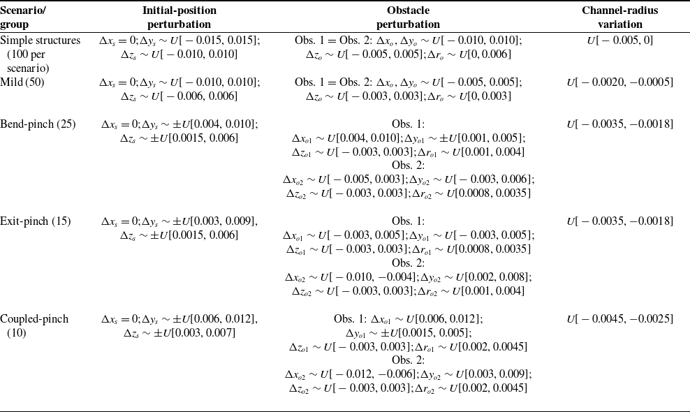
Perturbation variables, ranges, and sampling rules used in the randomized trials.

Table II. Long description

A table with six columns and six rows, detailing perturbation variables, ranges, and sampling rules for different scenarios. The columns are labeled Scenario/group, Initial-position perturbation, Obstacle perturbation, and Channel-radius variation. The table includes data for Simple structures, Mild, Bend-pinch, Exit-pinch, and Coupled-pinch scenarios. Each scenario lists specific perturbation variables and their sampling rules, with values given in meters. The table notes that denotes uniform sampling over and denotes a sampled magnitude with a randomly selected sign. Obstacle perturbations are listed in a specific order.

Note: ${U}[{a},{b}]$ denotes uniform sampling over $[{a},{b}] ; \pm {U}[{a},{b}]$ denotes a sampled magnitude with a randomly selected sign. Obstacle perturbations are listed in the order ( ${\unicode{x0394}} {x}_{\mathrm{o}},{\unicode{x0394}} {y}_{\mathrm{o}},{\unicode{x0394}} {z}_{\mathrm{o}},{\unicode{x0394}} {r}_{\mathrm{o}}$ ). The 100 complex-topology trials are divided into four perturbation bands: mild (50), bend-pinch (25), exit-pinch (15), and coupled-pinch (10). All quantities are in meters.

5.1. Scenario grouping and perturbation generation

The simulation evaluation is conducted across two scenario groups. The simple-structure group comprises six basic channel types: a straight channel with a single obstacle, an L-shaped bend, a narrow-gap channel, an S-shaped compound bend, a T-junction, and a cross-junction. These scenarios serve to evaluate the fundamental behaviors of the algorithms within typical geometric units. Conversely, the complex-structure group utilizes a realistic utility-tunnel topology – featuring a main corridor, two branches, local obstacles, and abrupt clearance changes – to assess traversal stability in a highly constrained environment representative of actual inspection sites. To ensure statistical robustness, 100 perturbed instances are generated for each of the six simple scenarios (totaling 600 trials), alongside another 100 instances for the complex topology. The perturbation tables are generated using a fixed random seed and are shared by all evaluated methods, ensuring that each method is tested on the same environment and initial-condition instances. Perturbations are strictly applied to the environmental geometry and initial conditions, whereas the internal parameters of each algorithm remain constant across the same experimental group. The perturbation variables, ranges, and sampling rules are summarized in Table II. All continuous perturbations are sampled from bounded uniform distributions. The master random seed is 20260409; fixed seeds of 20260420 and 20260438 are used to generate the simple-structure and complex-topology perturbation sets, respectively. The same pre-generated perturbation instances are reused for all compared methods.

Table III.

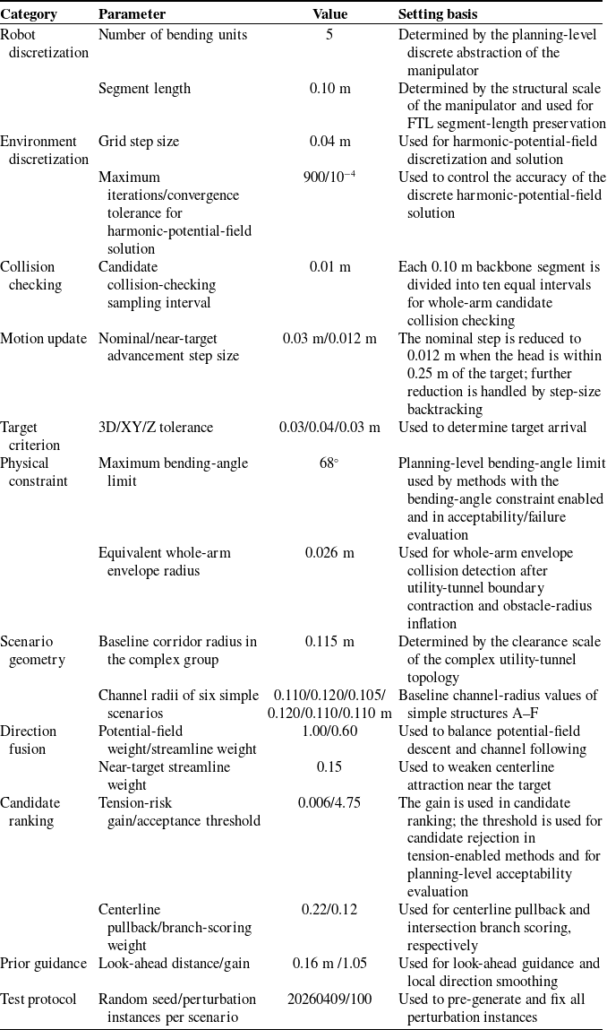
Core path planning parameters and selection rationale.

Table III. Long description

The table has 12 rows and 4 columns. The columns are labeled Category, Parameter, Value, and Setting basis. The categories include Robot discretization, Environment discretization, Collision checking, Motion update, Target criterion, Physical constraint, Scenario geometry, Direction fusion, Candidate ranking, Prior guidance, and Test protocol. Each row lists a specific parameter, its value, and the setting basis. For example, under Candidate ranking, the Tension-risk gain/acceptance threshold is 0.006/4.75, and the Centerline pullback/branch-scoring weight is 0.22/0.12. Under Prior guidance, the Look-ahead distance/gain is 0.16 m /1.05. Under Test protocol, the Random seed/perturbation instances per scenario is 20260409/100.

5.2. Comparative algorithms and implementation conditions

The comparative algorithms are categorized into two groups: baseline guidance methods and the proposed framework together with its ablated variants. All methods share the same FTL-based whole-arm propagation and collision-checking implementation, while the enabled guidance and configuration-evaluation modules differ according to the method definition. Specifically, APF utilizes the classical APF for head guidance; HF relies solely on the harmonic-potential-field gradient; and HF + CL combines the harmonic potential field with the centerline prior but lacks look-ahead capabilities, multicandidate searching, curvature constraints, and tension-risk evaluation. For the ablation studies, the proposed w/o κ retains the centerline prior, multicandidate search, and tension-risk term but does not apply the explicit bending-angle limit. Proposed w/o T maintains the curvature constraints and multicandidate search but excludes the tension-risk term. Finally, the proposed full method naturally integrates all the aforementioned modules. This categorization isolates the specific contributions of global guidance, candidate generation, curvature constraints, and tension-risk ranking, preventing the overall performance improvements from being overly attributed to any single module. For reproducibility, APF uses a repulsive gain of 0.18 and an influence range of 0.025 m. HF and HF + CL use the same harmonic potential field, with a maximum of 900 field iterations and a convergence tolerance of $10^{-4}$ . All methods use a nominal advancement step of 0.03 m and the same target-reaching criterion defined in Section 5.3. Whole-arm collision checking is performed at a sampling interval of 0.01 m along each backbone segment. No additional post-processing smoothing is applied to APF, HF, or HF + CL. To ensure a fair evaluation and eliminate discrepancies arising from parameter tuning, all methods are executed on identical scenarios and perturbation instances with standardized start and target points, environment grids, collision-checking resolutions, and iteration limits. The robot is uniformly modeled with five discrete bending units, each having a nominal length of 0.10 m. The grid step size is fixed at 0.04 m, with a nominal advancement step size of 0.03 m. The maximum iteration limits for the six simple-structure scenarios are set to 170, 180, 190, 190, 190, and 200, respectively, whereas the complex-structure group employs a uniform limit of 320 iterations. Under these standardized conditions, no method-specific parameter tuning is permitted beyond the explicit enabling or disabling of modules dictated by the algorithm’s definition. Consequently, the performance variations reported in the subsequent results stem fundamentally from the distinct candidate-configuration generation and screening mechanisms rather than operational discrepancies.

5.3. Parameter setup, success criteria, and failure classification

The core parameters listed in Table III are not separately tuned for different methods but are directly taken from the simulation code and scenario models. These parameters include the robot discretization parameters, harmonic-potential-field solution accuracy, step-size setting, curvature limit, centerline weight, and tension-risk gain. The baseline corridor radius for the complex topology is 0.115 m; the baseline channel radii for the six simple scenarios A–F are 0.110, 0.120, 0.105, 0.120, 0.110, and 0.110 m, respectively. The equivalent whole-arm envelope radius is set to 0.026 m and is used for collision detection after utility-tunnel boundary contraction and obstacle-radius inflation. The maximum bending-angle threshold of 68° is a planning-level candidate-screening threshold. It preserves the curvature margin under the current discretization length and advancement step size and does not represent the absolute hardware limit of the mechanism. By fixing these experimental conditions, the performance of different configuration-generation strategies can be compared more clearly under the same conditions.

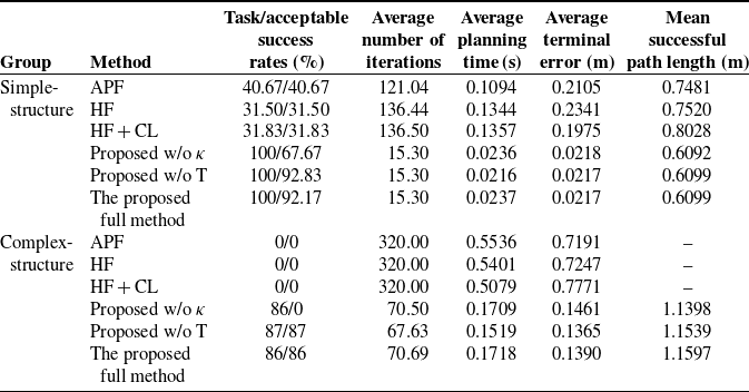
In a single trial, task success is recorded if the three-dimensional Euclidean distance from the head tip to the target is less than 0.03 m, or if the planar error is less than 0.04 m and the height error is less than 0.03 m. Acceptable success is evaluated more strictly over the generated configuration sequence. A task-successful trial is counted as acceptable only if it also satisfies the collision, bending-angle, clearance, and tension-risk criteria defined above. Therefore, task success measures target arrival, whereas acceptable success additionally measures planning-level configuration acceptability. Let $N_{\mathrm{all}}$ denote the total number of trials, and $N_{\rm succ}$ denote the number of task-success trials. The success rate is calculated as

(72) \begin{equation} R_{s}=\frac{N_{\text{succ}}}{N_{\mathrm{all}}}. \end{equation}

Success rate alone cannot distinguish different failure mechanisms. Therefore, failure types F1–F5 are assigned to task-unsuccessful trials using a fixed priority order. F5 denotes termination near a non-goal branch; F4 denotes failure to approach the target when the bending-angle limit is active and the maximum bending angle approaches the prescribed limit; F3 denotes collision-related failure identified from terminal collision or repeated collision rejection; F2 denotes stagnation identified from insufficient reduction of the goal distance over the terminal history window; and F1 denotes the remaining target-not-reached cases that do not satisfy the F2–F5 conditions. Trials that reach the target but do not satisfy the acceptable-success criterion are reported separately as acceptability failures and are not assigned an F1–F5 task-failure code.

5.4. Evaluation metrics

The performance of different planning methods is evaluated from four aspects. First, target arrival is assessed using the success rate and average terminal error. Second, search effort is assessed using the average planning time and average number of iterations. Third, collision behavior during advancement is assessed by recording the average number of collision rejections, minimum clearance margin, and centerline deviation. Finally, proximity of the configuration to mechanism boundaries is evaluated using the maximum bending angle and the average path length over successful trials. Path length is calculated only for successful trials to avoid the shorter residual trajectories produced by early termination in failed trials, which would otherwise distort the average path length.

Let $\min _{i}c({p}_{i}^{k,r})$ denote the minimum clearance at the $k$ -th step of the $r$ -th trial. The average minimum clearance can then be written as

(73) \begin{equation} \overline{d}_{\min }=\frac{1}{N_{\mathrm{all}}}\mathop{\sum }\limits_{r=1}^{N_{\mathrm{all}}}\min _{k}\min _{i}c\left({p}_{i}^{k,r}\right)\!. \end{equation}

Let $L_{\rm succ}$ denote the path-length set of successful trials. The mean successful path length is computed only over this set to characterize the geometric cost of successful traversal.

6.1. Results for the simple-structure scenarios

For the simple-structure group, Figure 8(a) shows the overall trends over 600 perturbed trials in six basic channel scenarios, and Table IV reports the corresponding main performance metrics. The full method, the method without the curvature term, and the method without the tension term all achieve a task success rate of 100%. Among them, the acceptable success rate is 92.17% for the full method, 92.83% for the method without the tension term, and 67.67% for the method without the curvature term. The full method has an average number of iterations of 15.30, an average planning time of 0.0237 s, an average terminal error of 0.0217 m, and a mean successful path length of 0.6099 m. The task success rates of APF, HF, and HF + CL are 40.67%, 31.50%, and 31.83%, respectively, and their average numbers of collision rejections are 110.12, 126.24, and 124.72, respectively. These results show that the baseline methods can still maintain a certain level of reachability in low-constraint scenarios such as straight corridors. However, in high-constraint scenarios such as sharp bends and intersections, the head guidance direction cannot be stably converted into whole-arm configurations satisfying the planning-level acceptability criteria, resulting in a significant increase in collision rejections.

Further analysis by scenario type shows that the performance degradation of the baseline methods mainly occurs in sharp-bend and intersection scenarios. In the straight-corridor scenario, the APF task success rate is 100%, while those of HF and HF + CL are 95% and 96%, respectively. In the narrow-gap scenario, APF reaches 100%, while HF and HF + CL reach 94% and 95%, respectively. In the S-shaped compound bend, APF decreases to 44%, whereas HF and HF + CL both drop to 0%. In the L-shaped bend, T-junction, and cross-junction scenarios, the task success rates of all three baseline methods are 0%, while the full method maintains a 100% task success rate in all six simple scenarios. This indicates that although the baseline methods can generate head guidance directions in some scenarios, they cannot ensure stable following of the remaining backbone segments or the acceptability of the whole-arm configuration after sharp turns or branch switching.

The gap between the task success rate and the acceptable success rate in Figure 8(a) indicates that task arrival is not equivalent to configuration acceptability. The average maximum bending angles of the full method, the method without the tension term, and the method without the curvature term are 42.48°, 42.44°, and 46.67°, respectively, all of which are generally below the bending-angle limit of 68°. However, in terms of acceptable success rate, the method without the curvature term achieves only 67.67%, which is significantly lower than 92.83% for the method without the tension term and 92.17% for the full method. This indicates that even when the average bending level does not exceed the threshold, some configurations that reach the target may still be judged unacceptable because of insufficient local curvature margin, clearance, or actuation margin.

6.2. Results for complex utility-tunnel topologies

The complex utility-tunnel topology shown in Figure 9 contains a main corridor, branches, local bends, and clearance contractions. Compared with the simple-structure group, it more easily exposes problems in whole-arm following and constraint screening. The results show that the proposed full method can advance progressively along the main corridor and maintain continuous evolution of the whole-arm configuration in the branch, local-bend, and clearance-contraction regions. The task success rates and acceptable success rates of APF, HF, and HF + CL are all 0%; their average numbers of iterations all reach the upper limit of 320; their average terminal errors are 0.7191, 0.7247, and 0.7771 m, respectively; and their average numbers of collision rejections are 312.00, 282.70, and 271.44, respectively. By contrast, the task success rates of the method without the curvature term, the method without the tension term, and the full method are 86%, 87%, and 86%, respectively, and their acceptable success rates are 0%, 87%, and 86%, respectively. The full method has an average number of iterations of 70.69, an average planning time of 0.1718 s, and an average terminal error of 0.1390 m.

Figure 9.

Configuration evolution sequence of the proposed full method in the complex topology.

The difference in acceptable success rate between proposed w/o ${\unicode{x03BA}}$ and the proposed full method in Figure 8(b) further indicates that the complex-structure group amplifies the influence of curvature constraints on final planning-level acceptability. After the curvature constraint is removed, the method without the curvature term achieves a task success rate of 86%, but its average maximum bending angle increases to 80.18°, exceeding the 68° planning limit. Its acceptable success rate is therefore 0%. The task success rate and acceptable success rate of the method without the tension term are both 87%, whereas those of the full method are both 86%. Their average maximum bending angles are 62.39° and 62.33°, respectively, both below the upper limit. In the complex-topology group, the mean of the per-trial maximum tension-risk proxy over 100 trials decreases from 0.4536 for the proposed w/o T to 0.4382 for the proposed full method. For each trial, the maximum value is taken over the generated configuration sequence before averaging across all trials. These values are dimensionless planning-level risk indicators rather than measured cable tensions. This difference indicates that the tension-risk term makes candidate ranking more conservative and may cause a small loss in geometric traversability, but it reduces the proportion of candidate configurations approaching the cable-drive actuation boundary.

6.3. Failure modes and mechanism interpretation

In the simple-structure group, all failures of APF, HF, and HF + CL are classified as F3, accounting for 59.33%, 68.50%, and 68.17% of all perturbed trials, respectively. In the complex-structure group, all 100 failures of APF are F3. For HF, F3 accounts for 91% and F2 for 9%; for HF + CL, F3 accounts for 87% and F2 for 13%. The method without the curvature term reaches the target in 86 trials, but the corresponding generated configuration sequences do not satisfy the bending-angle acceptability criterion, resulting in 0 acceptable successes; the remaining 14 trials that fail to reach the target mainly exhibit F2 stagnation. The method without the tension term and the full method have 13 and 14 F2 failures, respectively. In other words, the baseline methods usually provide a seemingly reasonable head direction, but this direction cannot be stably converted into a whole-arm configuration flow. The proposed method largely eliminates collision-type failures in complex topologies, and the remaining failures mainly arise from advancement stagnation near local contractions and branch-switching regions. The ablation results indicate that the observed improvement is produced by the complementary roles of the individual modules rather than by a single component. The curvature-related constraint primarily suppresses excessive local bending, whereas the tension-risk term biases candidate selection away from configurations with higher planning-level actuation risk. The centerline-guided multicandidate process mainly contributes to maintaining progress through branch and contraction regions.

These results show that physical constraints such as curvature, clearance, and cable-drive risk should be incorporated into candidate-configuration generation and screening at the planning level, rather than being left entirely to the execution layer. The method without the curvature term still achieves 86% geometric arrival in the complex-structure group, but its average maximum bending angle exceeds the upper bound, and its acceptable success rate is 0, indicating that geometric arrival is not equivalent to planning-level configuration acceptability. The method without the tension term has a slightly higher task success rate than the full method, showing that removing the tension-risk term relaxes the candidate acceptance criterion. The full method reduces the mean of the per-trial maximum tension-risk proxy from 0.4536 to 0.4382, corresponding to a more conservative planning-level actuation margin. The tension risk used here remains a planning-level proxy and cannot replace actual tension considering friction and transmission losses. To provide more intuitive evidence of process differences in the complex topology, Figure 10 compares representative results of the six algorithms in the same utility-tunnel topology.

Figure 10.

Configuration evolution comparison among six planning algorithms within the complex utility-tunnel topology.

APF, HF, and HF + CL experience collision or stagnation in the branch-constriction region. The method without the curvature term can continue advancing, but its local overbending exceeds the curvature limit. Both the method without the tension term and the full method complete acceptable traversal, while the full method further considers tension-risk ranking. Figure 10 provides spatial configuration evidence corresponding to the statistical trends in Figure 8(b), which reports the overall performance over 100 perturbed instances.