



1. INTRODUCTION
Schurz (Reference Schurz2008, Reference Schurz2009; most recently, Reference Schurz2018, Ms) proposes a justification of induction based on the provable optimality of meta-induction, induction at the level of competing methods of inference.
1.1 Schurz's proposal
The naive reply to the problem of induction is that induction is justified because it has been successful in the past. Naive, Hume showed, because this suggested justification must be circular: it requires the principle of induction itself. Either that, one can qualify, or it must rest on a higher principle of induction: the justification of object-induction at the level of observed events requires meta-induction at the level of inference methods (see Skyrms Reference Skyrms2000: 35ff). But then induction at this level would require justification, setting in motion an infinite regress.
Now Schurz's idea is essentially that this regress may be halted directly at the second level: his idea is that it is possible to give a purely deductive or analytic justification of meta-induction, induction at the level of methods. This deductive justification comes in the form of mathematical results on the optimality of meta-inductive strategies in the setting of sequential prediction, results from the field of prediction with expert advice (Vovk Reference Vovk, Fulk and Case1990, Reference Vovk1998; Littlestone and Warmuth Reference Littlestone and Warmuth1994; Cesa-Bianchi et al. Reference Cesa-Bianchi, Freund, Haussler, Helmbold, Schapire and Warmuth1997; for overviews see Vovk Reference Vovk2001; Cesa-Bianchi and Lugosi Reference Cesa-Bianchi and Lugosi2006; Grünwald Reference Grünwald2007: 573ff).
Furthermore, “this analytic justification of meta-induction would at the same time yield an a posteriori justification of object-induction in the real world: for we know by experience that in the real world, noninductive prediction strategies have not been successful so far, hence it would be meta-inductively justified to favor object-inductivistic strategies” (Schurz Reference Schurz2008: 282).
Schurz's proposal is a refinement of the basic idea behind Reichenbach's attempted vindication of induction (Reichenbach Reference Reichenbach1933: 421f, Reference Reichenbach1935: 479ff, Reference Reichenbach1938: 348ff, Feigl Reference Feigl and Black1950; see Salmon Reference Salmon1967: 52ff, 85ff; Skyrms Reference Skyrms2000: 44ff). This idea is that, while we cannot deductively show induction to be reliable or guaranteed to be successful, without the help of question-begging assumptions on the ‘uniformity of nature,’ we might be able to show deductively that induction is optimal : it is guaranteed to be successful, no matter the course of nature, if any method is.
1.2 Reichenbach's pragmatic justification
Reichenbach's proposal was based on a particular rule of induction, that was motivated by his thoroughly probabilistic epistemology and his frequentist interpretation of probability. This induction rule, best known as the straight rule, infers probabilities of future events through induction by enumeration: it estimates the limiting relative frequencies by the current relative frequencies.
Now Reichenbach's argument is as follows. Either nature is in fact uniform – a limiting relative frequency exists – or it is not. If it is, then the inductive method (the straight rule) will be successful: it will converge on the correct limiting frequency. If it is not, if no limiting relative frequency exists, then obviously no method will be successful in this sense. Hence the inductive method is successful if any strategy is.
Clearly, there are many weak spots in this argument. There is the sweeping reduction of scientific inference to estimating limiting relative frequencies (Sellars Reference Sellars1964: 212ff; Skyrms Reference Skyrms1965: 254ff); there is the fact that there are infinitely many other methods that are likewise guaranteed to be successful in converging to an existing limiting relative frequency (Reichenbach Reference Reichenbach1938; Salmon Reference Salmon1957). But most destructive to the argument is the fact that it is simply not true that no method can be successful if there is no limiting relative frequency (Herz Reference Herz1936). After all, event sequences that never converge on a particular relative frequency of events might still be successfully – even perfectly – predicted by one or another method: because such sequences might still have much structure, or indeed because we cannot exclude the ‘method’ of a clairvoyant with perfect foresight.
To this last objection Reichenbach (Reference Reichenbach1938: 357ff) replied that a successful such alternative method has a high relative frequency of successful predictions, which implies that his inductive method posits that this method's predictions will continue to be accurate (by enumerative induction the limiting relative frequency of this method's predictions being successful is inferred to be high). Reichenbach did not proceed to make this idea more precise, though: and indeed it does not seem feasible to reconcile the different levels at which his straight rule is now working – both the object-level of the events and the meta-level of other methods – in such a way that his strategy can be vindicated as desired (Skyrms Reference Skyrms1965: 260f, Reference Skyrms2000: 44ff; Schurz Reference Schurz2008: 281).
1.3 Schurz's proposal; this paper
By clearly separating object-induction on the level of events and meta-induction on the level of prediction strategies, Schurz manages to give a precise form to Reichenbach's fundamental observation that induction picks up the past success of alternative methods. By combining this with the empirical fact of the object-inductive strategy's success, Schurz claims to have derived a proper, noncircular justification of object-induction.
Can Schurz's proposal be considered successful? In this paper I work towards an answer by reconstructing the argument, and clarifying and filling in aspects that, I think, are somewhat opaque or missing in Schurz's own presentation. My conclusion will be that the argument, suitably explicated, goes a long way; but there are some qualifications. One qualification is the need for a very strong empirical postulate on the success of the scientific method, that, I will claim, we must identify the object-inductive strategy with. Another is that the argument cannot provide justification for the object-inductive strategy; at best it can give justification for following the object-inductivist, or the scientific method, for now. I also identify a subtle yet important issue having to do with the relevant pool of alternative strategies, that I leave for further investigation in a follow-up paper.
Another aim of this paper is to provide a brief and accessible overview of some main results and insights from prediction with expert advice. While this approach is as of yet little known outside of the theory of machine learning, its core ideas, particularly the optimality of aggregating experts’ predictions based on their past predictive success, promise to offer an interesting new perspective on opinion pooling in social epistemology (see Dietrich and List Reference Dietrich, List, Hájek and Hitchcock2016). In particular, I will embed these results in a more familiar Bayesian perspective.
1.4 Overview of this paper
First, in section 2, I will discuss the framework of sequential prediction, including the notion of prediction game (the specification of possible events and predictions, sect. 2.1, and a loss function, sect. 2.2), the goal of designing an optimal strategy (sect. 2.3), and its adequacy for studying the problem of induction (sect. 2.4). I will give special attention to the probabilistic prediction game.
Next, in section 3, I will give a detailed reconstruction of Schurz's argument. The first step (sect. 3.1) is the analytic optimality of meta-induction: here I will explain the relevant definitions of meta-inductive strategies and the relevant results regarding their optimality, and I will show how this body of theory can be understood as generalizing the Bayesian approach to prediction.
The second step (sect. 3.2) is the empirical success of object-induction: here I will discuss the problem of the description of induction, and argue for a high-level view where the object-inductive strategy is identified with scientific method, that stands in competition with various nonscientific methods.
The conclusion of Schurz's argument (sect. 3.3) is that the optimal meta-inductive strategy confers justification to the most successful strategy so far, the object-inductive strategy. Here I will, first, discuss whether the meta-inductivist's optimality actually amounts to a justification for it. Second, I will discuss whether justification for the optimal meta-inductive strategy indeed goes over to justification for object-induction. I conclude in section 4.
2. THE FRAMEWORK OF PREDICTION
In this section I set out and motivate the framework of sequential prediction that is presupposed throughout the paper. My presentation of this framework is fully based on existent theory, as reported in the textbook by Cesa-Bianchi and Lugosi (Reference Cesa-Bianchi and Lugosi2006) and in Schurz's papers. I stay as close as possible to Schurz's presentation and notation, but also deviate from it where I think this makes things more clear.
2.1 The prediction game: events and predictions
Schurz defines a prediction game as a pair (y ω, Π) of a history yω and a pool Π of prediction strategies. It makes sense to extend this definition to include a third component, the loss function; this I will discuss in sect. 2.2.
A history yω is an infinite sequence of events. Events are identified with values in some set Val of possible values; I will provide examples below. Write y n for the n-th element of yω, or the event in round n of the game ( $n\in {\open N}^{ > {\rm o}}$).
Predictions are elements in some set Valpred; again I will provide examples below.
A prediction strategy, an element of the pool Π, specifies in each round a prediction about the next event. Write predn(P) for the prediction of strategy P for round n.
Schurz in (Reference Schurz2008, Reference Schurz2009) discusses two different types of prediction games: the binary and the real-valued prediction game.
2.1.1 Example: the binary prediction game
Here the events can take one of two possible values, 0 and 1; and the predictions are simply categorical guesses about the possible values, 0 or 1. That is, Val = Valpred = {0, 1}.
This is the prediction game Schurz (Reference Schurz, Bluhm and Nimtz2004) discusses in an early exposition of his proposal. However, this simple prediction game is complicated in the sense that it is impossible to specify optimal strategies, as explained below. This is perhaps why Schurz in (Reference Schurz2008, Reference Schurz2009) also considers the following more general game.
2.1.2 Example: the real-valued prediction game
In this game both the events and the predictions take real values in the range [0, 1]. That is, Val = Valpred = [0, 1].
As explained in more detail below, for this game we can establish optimality results. The reason is that we can get the most out of hedging strategies, that predict by taking some weighted mean of the predictions of all the strategies in the pool: namely, for real-valued predictions, and unlike binary predictions, any weighted mean is still a valid prediction.
2.1.3 Example: the probabilistic binary prediction game
But this we can already achieve by allowing real-valued predictions in the binary prediction game. Formally this gives the game where Val = {0, 1} and Valpred = [0, 1].
A likely interpretation is that we have introduced the possibility of randomization in the binary prediction game: a prediction strategy now has access to a random device, which in each round it can use to toss a virtual coin with any desired bias p ∈ [0, 1], and give out prediction 1 if it lands heads and 0 if it lands tails. Note, however, that on this interpretation we are still in the categorical binary prediction game; the difference is that we have allowed prediction strategies to be random variables. Concretely, this means that the bounds we derive below are applicable to the binary prediction game only in expectation (see Cesa-Bianchi and Lugosi Reference Cesa-Bianchi and Lugosi2006: 67ff).
The alternative interpretation is that a strategy directly issues probabilistic rather than categorical predictions. That is, a prediction strategy issues elements in Valpred = [0, 1], where we interpret the latter as probabilities (for the next outcome being 1, say). In particular, the loss function scores the difference between the actual outcome and the issued probability, sect. 2.2 below.
This probabilistic binary prediction game constitutes, I think, a natural general framework of prediction (also see sect. 2.4 below). It is therefore noteworthy that this game does not receive much attention in Schurz's published papers: less attention, in any case, than possible ways of simulating the hedging strategy in the game where predictions must be categorical. Thus Schurz (Reference Schurz2017 828f, Reference Schurz2018: 3890) considers two possibilities: the aforementioned introduction of randomization (Schurz and Thorn Reference Schurz and Thorn2016: 48), and the use of a collective of meta-inductivists, the categorical predictions of which we then take the mean value of (Reference Schurz2008: 298ff, Reference Schurz2009: 214f). Schurz prefers the second solution to the interpretation of randomization, making the valid point that the latter “is not entirely general since it presupposes that the events are probabilistically independent from [the meta-inductivist's] choice of prediction,” (Reference Schurz2017: 828; cf. Shalev-Shwartz and Ben-David Reference Shalev-Shwartz and Ben-David2014: 252). Still, the introduction of a collective of meta-inductivists is ultimately a way of simulating single probabilistic predictions, and, due to rounding-off effects (see Schurz Reference Schurz2008: 299, Reference Schurz2009: 215), an imperfect way at that. It seems to me that both the choice of game and Schurz's choice of evaluating the mean success of a collective of strategies are modeling choices (cf. Schurz Reference Schurz2009: 215), that are less general and less elegant than evaluating the loss of a single meta-inductivist that is allowed probabilistic predictions.
2.2 The prediction game: the loss function
Strategy P , when making prediction predn(P) = pred ∈ Valpred for round n, suffers, when the outcome is revealed to be y n ∈ Val, a loss ℓ(pred, y n).
That is, a loss function ℓ: Valpred × Val → [0, ∞] quantifies how much a prediction was off in light of the actual outcome. Assuming that the function is nonnegative, that it returns 0 in case of the best possible prediction given the outcome, and that it is increasing in divergence between the prediction and the outcome, we are still left with much freedom in choosing a particular function.
2.2.1 Example: the zero-one loss function
Defined by ℓ0/1(pred, y) = 0 if pred = y and ℓ(pred, y) = 1 otherwise, this is an obvious loss function in the categorical binary prediction game.
2.2.2 Example: the absolute loss function
Defined by ℓabs(pred, y) = |pred − y |, and called the natural loss function by Schurz, this is indeed an obvious loss function in the real-valued prediction game. Note, moreover, that this function reduces to the zero-one loss function in the categorical binary prediction game.
The absolute loss function can, of course, also be used in the probabilistic binary prediction game. In fact, in the categorical prediction game that allows strategies the use of randomization, the p-expected zero-one loss coincides with the absolute loss ℓabs(p, y) = | p − y | evaluated on probabilistic prediction p ∈ [0, 1]. It is in this sense that one might say that the categorical binary prediction game with randomization and the probabilistic binary prediction game coincide. However, to repeat, the difference is that in the first case we are dealing with expected losses, whereas in the second case the loss function deals with probabilistic predictions directly.
The absolute loss function does fail to satisfy a usual requirement on loss functions in a probabilistic context. Namely, the absolute loss function is not proper : whenever p > 0.5 (respectively, p < 0.5), the p-expected loss of prediction q is minimized by the extreme prediction q = 1 (by q = 0), rather than by p itself.
2.2.3 Example: the square loss function
Defined by ℓsq(pred, y) = (pred − y)2, this loss function is proper.
2.2.4 Convex bounded loss functions
The absolute and the square loss function are both convex in their first argument: for all α ∈ [0, 1], predictions pred1, pred2 ∈ [0, 1] and outcomes y, it holds that
 $${\rm \ell} (\alpha \cdot{\rm pre}{\rm d}_{\rm 1} + (1-\alpha )\cdot {\rm pred}_{2},y{\rm )} \le \alpha\cdot \ell (\,{\rm pred}_{1},y) + (1-\alpha )\cdot \ell (\,{\rm pred}_{2},y).$$
In words, the loss of a prediction that is a weighted mean of several predictions, is no worse than the weighted mean of the losses of these individual predictions. This is an important technical property that underlies the below results on the existence of optimal strategies; strategies that indeed proceed by taking weighted averages of all available predictions.
The absolute and the square loss function are also bounded, meaning that their range is the interval [0, 1]. The first main optimality result that I discuss below (sects 3.1.2–3.1.4) covers all convex bounded loss functions.
2.2.5 Example: the logarithmic loss function
Defined by
 $$\ell _{\log} ({\rm pred},y) = \left\{ {\matrix{ {-\ln (1-{\rm pred})} & {{\rm if}\,y = 0} \cr {\!\!\!\!\!\!\!\!\!\!\!\!- \,{\rm ln }\;{\rm pred}} & {{\rm if}\,y = 1} },} \right.$$
this is a prominent loss function (Cesa-Bianchi and Lugosi Reference Cesa-Bianchi and Lugosi2006: 247ff), for its technical properties as well as its information-theoretic interpretation (see e.g. Grünwald, Reference Grünwald2007; Sterkenburg Reference Sterkenburg2018: 137ff), and, as I will discuss in sect. 3.1.6 below, for its strong connection to Bayesian prediction.
The logarithmic loss function is proper and convex, but it is not bounded. (Indeed, the loss of extreme prediction pred = 0 on outcome y = 1, and pred = 0 on y = 1, is infinity.) As such, it falls outside of the scope of the below optimality result on convex bounded loss functions – but this is no matter, because, as I will explain below too (sects 3.1.5–3.1.7), it actually enables stronger results.
2.2.6 Cumulative losses and loss rates
Schurz defines the score of strategy P in round n by s(predn(P), y n) := 1−ℓ(predn(P), y n), and the absolute success absn(P) of P by the conclusion of round n as the sum  $\sum\nolimits_{i = 1}^n {} $ s(predi(P), y i) of its scores up to n. It is, however, more usual and indeed more convenient to evaluate things directly in losses, so that I will rather consider the absolute or cumulative loss given by Lossn(P) :=
 $\sum\nolimits_{i = 1}^n {} $ ℓ(predn (P), y i). Likewise, I define (parallel to Schurz's success rate) the loss rate lossn(P) of P by n as the average Lossn(P)/n of its losses up to n.
2.3 The goal: an optimal strategy
Given a pool Π of prediction strategies, we aim to design a meta-inductive strategy MI that, having access to the predictions of all the other strategies, predicts in such a way that it is optimal with respect to Π. To a first approximation, strategy MI is optimal with respect to Π if by following it we will always do about as good as we possibly could have done, given that the strategies in Π represent what we could have done. In other words, MI is optimal if it will always be about as successful as the most successful strategy in the pool. Here ‘always’ means: on every history of events. Importantly, we make no assumption whatsoever on possible histories. Another way of saying this is that we aim to derive worst-case guarantees.
What should ‘about as successful’ mean? As a start, we can demand that MI is at least as successful as any P ∈ Π in the long run. Let us define (parallel to Schurz's maximal success rate) by minlossn := minP∈Π∪{MI} lossn(P) the minimum loss rate among all the strategies (including the meta-inductivist itself) by round n. Then we can demand that MI's loss rate – its average loss per round – converges to no more than the lowest loss rate achieved by any of the strategies, in the long run:
 $$ \lim\limts_{ {n \to \infty}} ({\rm loss}_{\it n}({\rm MI})-{\rm minloss}_{\it n}) = 0.$$
(Again, there is no mention of the actual history: this is because it should hold for all histories.)
We will see below that we can indeed design strategies that achieve (1), at least for finite Π. This is still, however, a relatively weak demand: long-run convergence does not guarantee anything about the performance of the meta-inductivist by any given finite time. It does not guarantee anything about performance in the short run – or the speed of convergence.
We can express speed of convergence in terms of a function f, that depends on n and inevitably also on the size K := |Π| of the pool of strategies, such that for all rounds n,
 $${\rm los}{\rm s}_n\lpar {{\rm MI}} \rpar \le {\rm minlos}{\rm s}_n + f\lpar {n,K} \rpar .$$
The function f bounds what we call the regret rate: it bounds MI's surplus loss rate up to n, as compared to the loss rate it would have incurred if it would always have mimicked the strategy in Π that was, in hindsight, the most successful up to n. The regret rate, to give an interesting optimality bound, needs to be decreasing in n (or it would not even guarantee (1)) – and the faster the better.
Work in the field of prediction with expert advice has indeed led to metainductive algorithms that satisfy (2) for quickly decreasing f (Cesa-Bianchi and Lugosi Reference Cesa-Bianchi and Lugosi2006). For the general class of convex bounded loss functions we can achieve an f(n, K) with a main term of the form  $\sqrt {\ln \,K/n} $ giving a regret rate that decreases in
 $1/\sqrt n $ (sects 3.1.2–3.1.4). Moreover, for an important subclass of convex loss functions, f is of the form (ln K)/n, giving a regret rate that decreases in 1/n (sects 3.1.5–3.1.7). The latter indeed entails a finite constant bound (only depending on K) on the difference between MIs and any P’s total losses, or, for any P, the cumulative regret relative to P (of MI for not having mimicked P from the start)
 $${\rm Regret}_n\lpar P \rpar : = {\rm Loss}_n\lpar {\rm MI} \rpar -{\rm Loss}_n\lpar P \rpar .$$
In all of the following, when I loosely use the term ‘optimality,’ it is these kind of short-run guarantees that I have in mind.
2.4 The prediction game and the problem of induction
The previous set out the framework of the prediction game. It is within the confines of this framework that Schurz's proposed justification of induction proceeds. But, of course, there is the concern that this framework of prediction falls short of capturing the essence of inductive inference, and so a justification within this framework falls short of the real goal: to justify inductive or scientific reasoning (cf. Arnold Reference Arnold2010: 591).
One can, to begin with, object that scientific inquiry consists not so much in producing forecasts as in inferring general conclusions: not so much in prediction as in the formulation and the confirmation of hypotheses and theories. One can thus object to the generality of the problem setting of prediction; one can further object to the way predictive inference is rendered in our framework. Dawid (Reference Dawid1984: 279), when introducing what is essentially our probabilistic prediction game under the header of “prequential forecasting,” is frank about its limitations: “[t]he data may arrive en bloc, rather than in a natural order; if they come from a time-series, it may be impossible, or not obviously desirable, to analyse them at every point of time, or to formulate one-step ahead forecasts; and the restriction whereby all uncertainty about the next observation is to be encoded in a probability distribution, while acceptable to Bayesians, may not appeal to others.”
Nevertheless, while there certainly is a case to be made that prediction is only a subsidiary part of science, there is also an important opposed tradition, indeed fashionable in many parts of machine learning today, that takes it that scientific inference ultimately comes down to inductive inference from particulars to particulars, or predictive inference. Moreover, while our framework certainly cannot accommodate everything there is to say about prediction, and particularly the choice of a loss function introduces an arguably highly context-dependent element, I think, and will assume in this paper, that the probabilistic prediction game, in which we can demonstrate the desired optimality for a wide class of loss functions, possesses a level of generality that lends significance to the conclusions we draw from it: ultimately, hopefully, an actual justification of induction.
3. THE ARGUMENT
The proposed justification of induction proceeds by two steps: an analytic proof that meta-induction, which favors the most successful available strategy, is an optimal strategy (sect. 3.1), and the empirical fact that object-induction has so far been the most successful strategy (sect. 3.2). From this is to follow the conclusion that the optimal strategy would now proceed object-inductively, thus justifying object-induction (sect. 3.3).
3.1 Step one: the analytic optimality of meta-induction
Here I explain the “mathematical-analytic” justification of meta-induction (Schurz Reference Schurz2008: 282), that amounts to the definition of a meta-inductive prediction strategy and a theorem about its performance. Again, my presentation of the relevant mathematics is fully based on existing results in the field of prediction with expert advice.
3.1.1 Towards optimality: follow the leader or hedge your bets?
The most straightforward meta-inductive strategy is the strategy that in each round simply issues the same prediction as the then most successful strategy in the pool (Schurz's “simple meta-inductivist,” Reference Schurz2008: 285ff; or “imitate-the-best,” Reference Schurz2009: 207; elsewhere also “follow-the-best-expert,” Cesa-Bianchi and Lugosi Reference Cesa-Bianchi and Lugosi2006: 41ff; or simply “follow-the-leader,” De Rooij et al. Reference De Rooij, Van Erven, Grünwald and Koolen2014: 1282). This simple strategy often works well; specifically, it approaches the leader's success if there are not too many alternations in which strategy is the leader (De Rooij et al. Reference De Rooij, Van Erven, Grünwald and Koolen2014: 1295; generalizing Schurz's observation, Reference Schurz2008: thm. 1; Reference Schurz2009: thm. 1, that it works well if from some round on one and the same strategy will always be best). However, in the worst case this strategy can be very bad. It is very bad in case of an adversarial history that forces an endless rapid change in which strategy is the best, so that the meta-inductivist is always switching to a strategy that will then issue a bad prediction, making it perform significantly worse than each strategy in the pool (Schurz Reference Schurz2008: 285ff; Schurz Reference Schurz2009: 208; De Rooij et al. Reference De Rooij, Van Erven, Grünwald and Koolen2014: 1282).
In fact, a similar kind of scenario shows that in the categorical binary prediction game, no meta-inductive strategy can be optimal. Namely, in the categorical game, recall, strategies must give as predictions either 0 or 1; so (assuming that in each round there are at least two strategies with different predictions) the meta-inductivist must each round wholeheartedly follow the predictions of some strategy or strategies, and an adversarial history can then make these strategies fail, while the others in the pool are in that round maximally successful. So already in the simplest scenario of the two constant strategies that always make the same prediction, an adversarial history can make the meta-inductivist fail in each round, whichever strategy it then follows, while clearly for each possible history at least one of the strategies must at least half of the time predict correctly (Cesa-Bianchi and Lugosi Reference Cesa-Bianchi and Lugosi2006: 67; Schurz Reference Schurz2008: 298f).
The method to avert such scenarios – a method unavailable in the categorical game, but unlocked in the probabilistic game – is to ‘hedge your bets.’ That is, you predict in each round by some weighted average of the predictions of all the elements in the pool. This gives the weighted-average meta-inductivist wMI defined by
 $${\rm pre}{\rm d}_{n{\rm + 1}}({\rm wMI}): = \sum\limits_{P\in \Pi} {} w_n(P)\cdot {\rm pred}_{n + 1}(P).$$
From this perspective (the “hedge setting,” De Rooij et al. Reference De Rooij, Van Erven, Grünwald and Koolen2014: 1282, in terminology going back to Freund and Schapire Reference Freund and Schapire1997), the challenge comes down to choosing appropriate weights. It turns out that, with the right choice of weights, that depend on the strategies’ losses, any adversarial history that inflicts a high loss rate on the meta-inductivist must also inflict a high loss rate on all the other strategies. That is, such a weighted-average meta-inductivist always keeps its regret rate low: it is an optimal strategy.
3.1.2 The attractiveness-weighted meta-inductivist
The weighted-average strategy first discussed by Schurz (Reference Schurz2008: 296, Reference Schurz2009: 213) is the attractiveness-weighted meta-inductivist, denoted awMI. The weight it assigns to strategy P after round n is determined by how much better P did in hindsight: what Schurz calls P’s attractiveness but what is better known as the meta-inductivist's cumulative regret Regretn(P) relative to P , defined by (3) in sect. 2.3 above. The attractiveness-weighted meta-inductivist only takes into account those P that actually were more successful than it; those that were not, hence would give regrets that are nonpositive, we can conveniently exclude with the help of the abbreviation (Regretn(P))+:= max{0, Regretn(P)}. The predictions of awMI are then defined, for  ${{\it n} \in {\opf N}} $, by
 $${\rm pre}{\rm d}_{n{\rm + 1}}({\rm awMI}) = \displaystyle{{\Sigma _{P\in \Pi} \,({\rm Regret}_n(P))_{+} \cdot \,{\rm pred}_{n + 1}(P)} \over {\Sigma _{P\in \Pi} \,{({\rm Regret}_n(P))}_ +}}. $$
(Where we can stipulate Regret0(P) = 1, say, for all P, so that in the first round these terms simply cancel out.) This is the weighted-average meta-inductivist (4) with weights
 $$w_n(P)=\displaystyle{{({\rm Regret}_n(P))_ +} \over Z},$$
where Z always denotes a normalization term, in this case Z = ΣP∈Π (Regretn(P))+.
One can show, for all bounded convex loss functions, that awMI satisfies the long-run convergence bound (1). Namely, one can show (Cesa-Bianchi and Lugosi Reference Cesa-Bianchi and Lugosi2006: cor. 2.1, Schurz Reference Schurz2008: thm. 4, Reference Schurz2009: thm. 2) that awMI satisfies the bound (2) for f of order 1/√n; specifically, for all bounded convex loss functions,
 $${\rm los}{\rm s}_n({\rm awMI}) \le {\rm minloss}_n + \sqrt {\displaystyle{K \over n}.} $$
3.1.3 Improvements: polynomial weights
As noted by Schurz (Reference Schurz2008: 297), the attractiveness weighted strategy is a special case of the polynomially-weighted-average strategy in Cesa-Bianchi and Lugosi (Reference Cesa-Bianchi and Lugosi2006: 12), where the unnormalized weights are given by
 $$({\rm Regret}_n(P))_ + ^\eta $$
for some parameter η ≥ 1. Indeed, the bound (7), hence the worst-case speed of convergence, can be improved by a different choice of parameter. In the words of Cesa-Bianchi and Lugosi (Reference Cesa-Bianchi and Lugosi2006: 13, notation mine), “The choice η = 1 yields a particularly simple algorithm. On the other hand, the choice η = 2 ln K − 1 (for K > 2) … leads to lossn(awMI) ≤ minlossn + 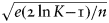 $\sqrt {e(2\,{\rm ln}\,K{\rm - 1})/n} $, yielding a significantly better dependence on the number of experts K.” Namely, the factor in the bound introduced by the size of the pool is now only its logarithm.
3.1.4 Improvements: exponential weights
The central strategy in the field, however, is the exponentially-weighted-average strategy, that employs unnormalized weights of the form
 $${\rm exp}(\eta \cdot {\rm Regre}{\rm t}_n(P))$$
for parameter η > 0 (the weighted-majority algorithm, Littlestone and Warmuth Reference Littlestone and Warmuth1994; see Cesa-Bianchi and Lugosi Reference Cesa-Bianchi and Lugosi2006: 14f; Shalev-Shwartz and Ben-David Reference Shalev-Shwartz and Ben-David2014: 252ff; and Schurz Reference Schurz2009: 214; Schurz and Thorn Reference Schurz and Thorn2016: 52). Note that (9) equals
 $${\rm exp}(\eta \cdot ({\rm Los}{\rm s}_n\lpar {{\rm wMI}} \rpar -{\rm Los}{\rm s}_n(P))) = {\rm exp}(\eta \cdot {\rm Los}{\rm s}_n\lpar {{\rm wMI}} \rpar )\cdot {\rm exp}(-\eta \cdot {\rm Los}{\rm s}_n\lpar P \rpar ),$$
and the first factor exp(η · Lossn(wMI)) cancels out in the normalization. Consequently, the choice of unnormalized weights (9) is equivalent to the choice
 $${\rm exp}(-\eta \cdot {\rm Los}{\rm s}_n(P)).$$
The exponentially-weighted strategy thus has the special property that its weights and hence its predictions only depend on the other strategies’ past successes, and not also on its own past success (Cesa-Bianchi and Lugosi Reference Cesa-Bianchi and Lugosi2006: 14).
Parameter η is also called the learning rate: the larger it is, the greater the inflation of differences in losses, and the more aggressive the updating. In this case the optimal way of tuning the parameter η is to let it decrease in a specific way in the number of rounds (Cesa-Bianchi and Lugosi Reference Cesa-Bianchi and Lugosi2006: 17f). This still gives a bound with a main term of the form  $\sqrt {\ln \,K/n} $ , which is indeed provably the best we can hope to achieve in general for the convex bounded loss functions (See Cesa-Bianchi and Lugosi Reference Cesa-Bianchi and Lugosi2006: 62f).
3.1.5 Improvements for other loss functions
The very strongest bound we could ever hope to derive, whatever the loss function, is of the form (c ln K)/n for some constant c – that is, a bound of order 1/n. Namely, for any given loss function, one can design a pool of experts and a history such that any meta-inductive strategy's loss rate falls at least this much short of the best strategy's (see Cesa-Bianchi and Lugosi Reference Cesa-Bianchi and Lugosi2006: 59ff).
As a matter of fact, we can derive this guarantee for a particular class of loss functions, that includes, among others, the quadratic and the logarithmic loss. I will now first discuss the important particular case of optimal probabilistic prediction with the logarithmic loss function, which is all the more interesting for its natural Bayesian interpretation.
3.1.6 The Bayesian meta-inductivist and the logarithmic loss function
In the probabilistic binary prediction game, recall from sect. 2.1.3, strategies in each round issue a probability pred ∈ [0, 1] of the next outcome being 1. As such, they can be seen to give conditional likelihoods (where n in ℕ, y n denotes the event sequence up to round n, and by stipulation P( .· | y0) := P( . ))
 $$P(y_{n + 1} \vert {\bi y}^n) = \left\{ {\matrix{ {1 - {\rm pre}{\rm d}_{n{\rm + 1}}(P)} & {{\rm if}\,y_{n + 1} = 0} \cr \hskip-15pt{{\rm pre}{\rm d}_{n{\rm + 1}}(P)} & {{\rm if}\,y_{n + 1} = 1} \cr},} \right.$$
and so, by the chain rule of conditional probabilities
 $$P({\bi y}^n): = \prod\limits_{i = 0}^{n-1} {} P(y_{i + 1} \vert {\bi y}^i),$$
likelihoods over finite histories (Cesa-Bianchi and Lugosi Reference Cesa-Bianchi and Lugosi2006: 247f).
The Bayesian meta-inductivist P BayMI maintains a probability model over both the space of possible histories and the pool of strategies. First, the marginal prior probability of each of the strategies is stipulated by some initial weight function w 0; thus P BayMI(P) := w 0(P). Second, the strategies’ likelihoods are stipulated to determine conditional probabilities P BayMI(yn | P) := P (yn) of histories. This, then, suffices to determine the marginal prior probability of histories. Namely, via the law of total probability we have
 $$P_{{\rm BayMI}}({\bi y}^n) = \sum\limits_{P\in \Pi} {} w_0(P)\cdot P{\rm (}{\bi y}^n{\rm )}{\rm.} $$
Now the Bayesian meta-inductivist's predictions for round n + 1 are, by Bayes's rule, simply given by the conditional probabilities on the past events by n,
 $$ P_{\rm BayMI}(y_{n{\rm + 1}} \vert {\bi y}^n) = \displaystyle{{P_{\rm BayMI}({\bi y}^{n + 1})} \over {P_{\rm BayMI}({\bi y}^n)}}.$$
Alternatively but equivalently (cf. Grünwald Reference Grünwald2007: 77), for each round n + 1 we can first calculate the posterior marginal probabilities by this round, identified with the weights w n by this round, that the Bayesian meta-inductivist assigns to the strategies. By Bayes's rule, we update the new weights after round n to
 $$w_n(P): = w_{\rm 0}(P \vert {\bi y}^n) = \displaystyle{{w_0(P)\cdot P({\bi y}^n)} \over Z},$$
with normalization  $Z = \sum\nolimits_{P\in \Pi} {} w_0(P)\cdot P{\rm (}{\bi y}^n{\rm )}$. Then by the law of total probability
 $$P_{{\rm BayMI}}(\cdot \vert {\bi y}^n) = \sum\limits_{P\in \Pi} {} w_n(P)\cdot P{\rm (}\cdot {\rm \vert} \,{\bi y}^n{\rm )}{\rm.} $$
In particular,
 $${\rm pre}{\rm d}_{n{\rm + 1}}({\rm BayMI}) = \sum\limits_{P\in \Pi} {} w_n(P)\cdot {\rm pred}_{n + 1}(P).$$
In short, the Bayesian meta-inductivist for the probabilistic prediction game is the weighted-average meta-inductivist with weights given by Bayes's rule, (15).
An important difference, at first sight, from the attractiveness-weighted meta-inductivist awMI, is that the weights of BayMI depend on the strategy's probabilistic predictions and so only indirectly on their losses. However, the Bayesian meta-inductivist is strongly connected to the logarithmic loss function (Cesa-Bianchi and Lugosi Reference Cesa-Bianchi and Lugosi2006: 247ff), which can be seen by writing out
 $$\eqalign{{\rm Los}{\rm s}_n(P) & = \sum\limits_{i = 0}^{n-1} {} \ell ({\rm pred}_{i + 1}(P),y_{i + 1}) \cr & = \sum\limits_{i = 0}^{n-1} {} -\ln \,P(y_{i + 1} \vert \,{\bi y}^i) \cr & = -\ln \prod\limits_{i = 0}^{n-1} {} P(y_{i{\rm + 1}} \vert \,{\bi y}^i) \cr & = -\ln P({\bi y}^n).} $$
That is, for the logarithmic loss, P(y n) = exp(−Lossn(P)). Substituting this term in the weight specification (15), we obtain
 $$w_n(P) = \displaystyle{{w_0(P)\cdot {\rm exp}(-{\rm Loss}_n(P))} \over Z}.$$
Another apparent difference with wMI is that BayMI still explicitly depends on the prior weights given by w 0. However, since we assume a finite pool, we can choose uniform prior weights w 0(P) = 1/K, in which case they all cancel out and we finally obtain
 $$w_n(P) = \displaystyle{{{\rm exp}(-{\rm Loss}_n(P))} \over Z}.$$
In words, the (uniform-prior) Bayesian meta-inductivist for the logarithmic loss function is the exponentially-weighted meta-inductivist introduced in sect. 3.1.4 above, with parameter η = 1 (Cesa-Bianchi and Lugosi Reference Cesa-Bianchi and Lugosi2006: 250).
Now it is easy to derive a bound on Lossn(BayMI) = − ln P BayMI(y n), using the simple fact that  $\sum\nolimits_{P\in \Pi} {} w_0(P)\cdot P({\bi y}^n) \ge w_0(P)\cdot P{\rm (}{\bi y}^n{\rm )}$ for any particular strategy P (Cesa-Bianchi and Lugosi Reference Cesa-Bianchi and Lugosi2006). Namely,
 $$\eqalign{{\rm Los}{\rm s}_n({\rm BayMI}) & = -{\rm ln}\sum\limits_{P\in \Pi} {} w_0(P)\cdot P{\rm (}{\bi y}^n{\rm )} \cr & \le -\ln \,(w_{\rm 0}(P)\cdot P{\rm (}{\bi y}^n{\rm )}) \cr & = -\ln \,w_0(P) + {\rm Loss}_n(P).} $$
In particular, with uniform choice of initial weights, we have for the loss rate that
 $${\rm los}{\rm s}_n({\rm BayMI}) \le {\rm minloss}_n + \displaystyle{{\ln \,K} \over n}.$$
3.1.7 Mimicking the Bayesian meta-inductivist for other loss functions
In the same way that we evaluated the cumulative loss
 $${\rm Los}{\rm s}_n({\rm BayMI}) = -{\rm ln}\sum\limits_{P\in \Pi} {} w_0(P)\cdot {\rm exp}(-{\rm Loss}_n(P))$$
in the special case of the Bayesian meta-inductivist with the logarithmic loss (the exponentially-weighted strategy with η = 1), we can, for any given loss function ℓ, as well as any learning rate η > 0, evaluate the term
 $${\rm MixLos}{\rm s}_n: = -1/\eta \cdot {\rm ln}\sum\limits_{P\in \Pi} {} w_0(P)\cdot {\rm exp}(-\eta \cdot {\rm Loss}_n(P)),$$
the so-called cumulative mix-loss. In particular, much like before, we can derive for any loss function that
 $${\rm MixLos}{\rm s}_n \le -1/\eta \cdot \ln w_0(P) + {\rm Los}{\rm s}_n(P),$$
so that, for uniform weights, the mix-loss rate satisfies
 $${\rm mixlos}{\rm s}_n \le \min \!{\rm los}{\rm s}_n + \displaystyle{{\ln K} \over {\eta \cdot n}}.$$
But what does this actually mean? Well, for some loss functions ℓ, the term (22), the mix-loss, is strictly meaningless, which is to say that there is no actual (meta-inductive) strategy that this cumulative loss term corresponds to. But for an important subclass of convex loss functions, the so-called mixable loss functions, and the right choice of η, the mix-loss (22) corresponds to an actual strategy (the aggregating strategy due to Vovk Reference Vovk, Fulk and Case1990, also see Vovk Reference Vovk1998, Reference Vovk2001; Cesa-Bianchi and Lugosi Reference Cesa-Bianchi and Lugosi2006: 52ff; Grünwald Reference Grünwald2007: 573ff; Sterkenburg Reference Sterkenburg2018: 143ff). This meta-inductive strategy aMI can be seen as explicitly mimicking the Bayesian strategy with the logarithmic loss function, for this loss function, with the aim of achieving the Bayesian performance bound (20). And indeed, virtually by definition, aMI is optimal for the given mixable loss function in the strong sense of (24).
The mixable loss functions include such important functions as the logarithmic loss (obviously: the mix-loss with η = 1 is the Bayesian strategy) and the square loss, but not the absolute loss function.
3.1.8 Summary
We have considered a number of central meta-inductive strategies for general classes of loss functions. These meta-inductive strategies are optimal for the relevant prediction games; they not only satisfy long-run convergence to the minimal loss rate among all strategies in the pool, but indeed short-run bounds of order  $1/\sqrt n $ (for the convex bounded loss functions) or even of order 1/n (the mixable loss functions).
We also saw that all of these optimal meta-inductive strategies are weighted-average strategies (or, for some mixable games, aggregating strategies), that predict by combining weighted predictions of all the other strategies in the pool. We indeed saw that the exponentially-weighted strategies (optimal for the convex bounded loss functions) and the aggregating strategies (for the mixable loss functions) can be understood as generalizations of the standard Bayesian strategy for the specific case of the logarithmic loss function.
Moreover, the assigned weights in all cases depend on the strategies’ losses, that is, on their past performance. Now in the Bayesian case the weights also depend on a prior weight assignment w 0, and we can introduce such a prior weight factor in the other meta-inductive strategies, too (see e.g. Cesa-Bianchi and Lugosi Reference Cesa-Bianchi and Lugosi2006: exc. 2.5): but the effect of these weights cancels out in case of a uniform prior over the finite pool of strategies, and I will assume this to be the reasonable choice (see sect. 3.3.1 below). Under that stipulation, the weights depend on the strategies’ performance only, and strategies that have been more successful receive a higher weight and have a larger share in the meta-inductivist's prediction. It is in that sense that we can say that the meta-inductive strategy favors strategies to that extent in which they have been more or less successful than the other strategies so far.
Thus, abstracting away from which of the standard loss functions we are actually assuming, and hence which precisely is the strategy that we will now simply call ‘the meta-inductive strategy MI,’ we can formulate the first, analytic step of Schurz's argument as
(A)
The meta-inductive strategy MI, that at each point in time favors strategies to the extent of their relative success so far, is an optimal strategy.
3.2 Step two: the empirical success of object-induction
The second step is the empirical observation that “so far object-induction has turned out to be the most successful prediction strategy” (Schurz Reference Schurz2008: 304).
3.2.1 The object-inductive strategy?
The problem of the justification of induction looks much intertwined with that of the description of inductive method (see Goodman Reference Goodman1954: 68ff; Skyrms Reference Skyrms2000: 51ff; Lipton Reference Lipton2004: 7ff). Thus Schurz in (Reference Schurz2004) starts by asking “which inductive method should be attempted to justify,” and then notes that “there is a fundamental method that more or less underlies all particular inductive methods – the straight rule” (243, translation mine). In subsequent papers (Reference Schurz2008: 283f, 300f; Reference Schurz2009: 206), Schurz also discusses the straight rule and refined version thereof.
Even if Schurz's purpose here is merely to illustrate some basic inductive strategies and how to refine them in more complex environments, it does bring out the worry that the proposed meta-inductive justification is conditional on some satisfying solution to the problem of description. But this is itself a fundamental problem; certainly any conception of object-induction as some variant of the straight rule directly faces Goodman's observation that induction is underdetermined in which past regularities are actually extrapolated. Of course, we have assumed a set of possible events, and the straight rule extrapolates the past relative frequencies of these events; but that merely shifts the problem to whether and how we have managed to carve out possible events in the world that are indeed extrapolatable or projectible in this way. Schurz (Reference Schurz2008: 279) writes, “I will avoid Goodman's ‘new riddle’ of induction by assuming that the events are explicated in terms of qualitative predicates or function symbols in the sense of Carnap (Reference Carnap1947: 146).” But this is a weak response: Carnap's reply was found wanting from the start (Goodman Reference Goodman1947, Reference Goodman1954: 78ff; Putnam Reference Putnam and Goodman1983: xf).
3.2.2 Meta-induction and entrenchment
So how to deal with the problem of description in the context of Schurz's proposed justification? I can see two possible ways out.
One is to face the problem of description head-on. Perhaps the optimality of meta-induction can be employed to found an account of projectibility of regularities in terms of their past successful projections or their entrenchment, much in the spirit of Goodman's own suggestions (Reference Goodman1954: 84ff). Thus the pool of prediction strategies is taken to represent the candidate projectable regularities, and we are meta-inductively justified to favor the strategy most successful so far, or the regularity best entrenched. Of course, this is all fairly speculative: much more work would need to be done to make this idea precise, and I will not attempt to do that in this paper.
3.2.3 The scientific method
Rather, my proposed way out goes to the other extreme: I will argue that in the context of Schurz's argument, we can simply disregard the problem of description.
What is crucial for the force of Hume's skeptical argument is that it goes through for any inductive method one could propose. The problem of induction can therefore actually be stated quite independently of the problem of description (Lipton Reference Lipton2004: 11). But something similar holds for Schurz's constructive argument. The argument does not rely on any specific characteristics that the object-inductive method might or might not have–it only relies on its past success. For Schurz's proposed justification of induction it is enough to accept that there is something like an inductive method, and that it has been successful in the past.
In fact, it is fair to say that the problem of induction derives much of its relevance from the identification of induction with scientific method, which turns the problem of induction into the problem of providing rational grounds for scientific procedure. This would indeed “not only be of fundamental epistemological importance; it would also be of fundamental cultural importance as part of the enterprise of enhancing scientific rationality (Schurz Reference Schurz2008: 280; see, especially, Salmon Reference Salmon1967: 54ff on the significance of the problem of induction). Now most of us will agree that there is something like scientific method, despite the fact that it is notoriously hard to make perfectly precise what it consists in. There is such a thing – and it can be distinguished from several nonscientific approaches (like consulting horoscopes, or accepting the forecasts of demagogues). Moreover, most of us will agree that science's past predictions have been quite successful – more successful at least than the past predictions of these alternative methods. Then the major challenge is to turn this fact of science's past success into a convincing argument for sticking to it, rather than turning to alternative methods.
And this is what Schurz's argument promises to do. Adopting a high-level perspective, where we take as object-inductive strategy OI the scientific method, which we further take to stand in competition with a pool Π of alternative nonscientific strategies, we plausibly have the empirical fact that OI has been most successful so far; and the promise of Schurz's argument is that this can then be plugged in with the analytic optimality (A) to lead to the desired justification of the scientific method.Footnote 1
3.2.4 Summary
In short, I take the second step to be that
(E)
As a matter of empirical fact, the object-inductive strategy OI, that we identify with the scientific method (and that we take to be in competition with various proposed nonscientific methods), has been, at this point in time, the most successful prediction strategy (among the pool Π of all of these competing strategies).
3.3 Conclusion: meta-induction favors object-induction
From the analytic observation (A) and the empirical observation (E) it follows that
(C)
The meta-inductive strategy MI for the pool Π of OI and its nonscientific competing strategies, an optimal strategy for Π, favors most, at this point in time, the object-inductive strategy OI.
Does conclusion (C) amount to the desired justification of OI? Only if we are clear about at least two additional things: (1) the optimality of MI in fact amounts to a justification for MI, and (2) the justification for MI is conferred to the strategy that it favors most, in particular, OI.
3.3.1 The justification for an optimal strategy
An initial worry is that a Reichenbachian optimality justification, in its original form often referred to as the pragmatic justification of induction, is only that: a pragmatic justification. In my view, however, this denotation is a misnomer, insofar it suggests that a ‘pragmatic’ justification is not a proper, epistemic, justification. While a justification from optimality falls short of a justification from reliability, guaranteed success, it is still an epistemic justification: guaranteed success whenever success can be achieved at all. (Cf. Schurz Reference Schurz2008: 282.)
Of course, this presupposes that we use an epistemically relevant notion of success. In the previous we equated success with low losses, and then made the notion of optimality precise in term of long-term and short-term relative success, or long-term and short-term constraints on the regret.
Now success whenever success can be achieved at all in the long run, or asymptotic convergence to a regret rate of 0, already gives a nontrivial notion of optimality. It cannot be attained, over all possible pools, by any purely object-inductive strategy which predictions will not depend on the other strategies in the given pool. This is essentially what Schurz calls the dominance of meta-induction over object-induction (Reference Schurz2017: 829f); and he writes that Reichenbach “has pointed out that already the optimality argument may be considered as a sufficiently strong justification of meta-induction, insofar as meta-induction is the only prediction strategy for which optimality can be rationally demonstrated” (Schurz Reference Schurz2008: 303).
Recall, though, that Reichenbach's own notion of long-run optimality included infinitely many different strategies, and this is also the case for our notion. Concretely, given an optimal strategy, we can devise infinitely many other strategies that up to any given round issue any given predictions, before settling on the same predictions as the original strategy. (Thus we can, for any given amount of cumulative loss, devise a strategy that initially incurs at least this amount of loss on some history, yet that is still optimal.) That means that if we seek justification for an optimal strategy's actual predictions, which will be relevant for the next step of deriving justification for following OI's predictions, sect. 3.3.2 below, then the long-run criterion is not enough. If a strategy's actual predictions were justified solely by virtue of the strategy's long-run success, then by the above we would have the perverse result that in each round any possible prediction is justified (cf. Salmon Reference Salmon1957).
Fortunately, the short-term regret bounds for meta-inductive strategies exclude the possibility of arbitrary short-time regrets, hence predictions. To appreciate how restrictive they are (and the resulting notion of optimality is), let us have a closer look at the motivation for the nature of these bounds, particularly, their twofold uniformity.
First of all, the loss bound (2) is for the various meta-inductive strategies derived from the guarantee
 $${\rm los}{\rm s}_n({\rm wMI}) \le {\rm loss}_n(P) + f\,{\rm (}n{\rm,} \,K{\rm ),}$$
for all P ∈ Π, i.e. from a bound that is uniform over all strategies. This is also connected to the choice of uniform initial weights w 0 for the weighted-average (or aggregating) meta-inductivist. With nonuniform initial weights we would have long-run optimality as before, and we would even have short-term guarantees, but not of the uniform kind: in the short-term bound the term K would be replaced by a strategy-dependent term 1/w 0(P). With nonuniform weights, we must have assigned some strategies weights strictly smaller than 1/K, which translates in a worse guarantee relative to these strategies, or a suboptimal performance if one of these strategies turns out to be the most successful. In short, a uniform bound presents the strongest possible single guarantee, independent of which strategy is most successful. And the choice of uniform weights is not just arguably the most reasonable choice in that the meta-inductivist should treat all competing strategies initially on a par, or should later evaluate strategies on their success only (sect. 3.1.8 above); it is the reasonable choice in that it comes with the strongest possible uniform short-term optimality guarantee.
Second of all, short-term optimality is a worst-case or uniform notion over all possible histories, as stipulated in sect. 2.3 above. But one can think of other ways of defining optimality in terms of loss bounds that are uniform over strategies yet nonuniform over possible histories. Specifically, one can define a notion of optimality that allows a somewhat looser all-cases relative loss rate bound in return for a much stricter bound in specific cases of particularly regular or easy data. However, such a notion must be motivated by a ruling that some possible histories are somehow more likely or more relevant than others: as such, it constitutes an assumption that some possible uniformities hold a privileged status. But the elegance of Schurz's argument is precisely that it promises a justification of induction without any uniformity-of-nature assumptions. In particular, the first step, on the optimality of meta-induction, should be free of such assumptions. And for this, worst-case optimality, a uniform bound over every possible history, appears the right notion.
Now, if we accept this requirement of uniform optimality, we can directly define the very best possible meta-inductive strategy, for a given loss function, as that strategy that (for a given pool of strategies) minimizes the worst-case regret for all strategies and all histories (the minimax regret; Cesa-Bianchi and Lugosi Reference Cesa-Bianchi and Lugosi2006: 30ff). This theoretical strategy then gives the absolutely optimal predictions, for the given loss function; and if we take these predictions to be thereby fully justified, then results on various extents to which the absolutely optimal minimax regret coincides with the short-term optimality bounds we discussed (Cesa-Bianchi and Lugosi Reference Cesa-Bianchi and Lugosi2006: 59ff; 252ff) show that our meta-inductive strategy's actual predictions are to various extents justified, too.
I will not go further into the mathematical specifics, though, because the analytical details of the question of justification ultimately cannot (and need not) be separated from the empirical context of Schurz's argument. It is, for instance, sufficient for the argument to connect justification to a notion of optimality that is strong enough that all optimal strategies give, at this point in time, a sufficiently high weight to the object-inductive strategy, which is at least partly an empirical question: we will discuss this next, in sect. 3.3.2.
Furthermore, the notion of optimality is, of course, a relative notion, relative to a particular pool of strategies. That means that an optimal strategy can only be justified insofar the original choice of pool of strategies is appropriate, a proper rendition of all we could do. Now it seems there is an obvious such pool in the context of Schurz's argument, namely the pool of proposed alternative strategies that figures in the empirical step (E). But this may actually not settle it; I return to this important point in the conclusion of the paper, sect. 4.
3.3.2 The justification for a strategy favored most by an optimal strategy
Suppose that we are justified in predicting with the optimal strategy MI, at each point in time, and given, by (E), that optimal strategy MI, at this point in time, favors most the object-inductive strategy OI. Now it sounds plausible enough that we are justified in favoring OI, at this point in time. But this is not yet a justification for strategy OI.
To begin with, there is a difference between actually following and merely favoring a strategy, at any point in time. That a meta-inductivist assigns the highest weight to a strategy does not entail that their predictions coincide. For instance, the meta-inductivist might give a much higher weight to OI than to each of a large number K of competitors; but those competitors might collectively still take up most of the weight and issue a prediction opposed to the one issued by OI, so that the prediction issued by the meta-inductivist is also very different from OI's. In that case it sounds implausible that MI confers justification to following OI's prediction.
Note, however, that such cases are excluded with a sufficiently strong empirical step (E). They are excluded by an (E) that says that, as a matter of empirical fact, the strategy OI has been so much more successful than its competitors, that the meta-inductivist attributes it such a large share of the total weight that its prediction (approximately) coincides with OI's prediction. Indeed, in that clear-cut case all optimal strategies would (approximately) give this same prediction, resolving remaining doubts about the justification for the specific predictions of either of them (sect. 3.3.1 above). Since following MI's prediction is then justified, following OI's prediction, being (approximately) the same prediction, is justified, too. Thus a sufficiently strong (E) resolves the problem; but, of course, it remains up for debate whether, as a matter of empirical fact, OI has really been that successful (cf. Schurz Reference Schurz2018: 3891).
This leads us to the final observation that we would at best have a justification for following OI's current prediction, which is not the same as a justification for the strategy OI. Here it clearly shows in what way Schurz's argument for the justification of object-induction is more subtle than trying to establish that object-induction is itself optimal, the original idea of Reichenbach (cf. Schurz Reference Schurz2008: 281). Strategy OI is, again, not itself optimal. In order to still conclude that we are justified, from this point on, in always following strategy OI, we would need to establish that the optimal strategy from this point on always favors OI. This would be the case if OI from this point on is always (much) more successful than its competitors: but observation (E), that OI has been the most successful so far, does not, of course, entail that. We can easily come up with possible futures in which OI loses its edge and some competitor strategy predicts vastly better (and so MI ceases to favor OI): this is just the failure of the naive meta-inductive justification of induction.
Thus Schurz's argument, if successful, only gives a justification for sticking to strategy OI for now : it only gives a justification for following its prediction at this point in time.Footnote 2 This is, to reiterate, strictly weaker than a justification for object-induction, which is normally understood as a justification for always following the strategy OI. Nevertheless, this would still be an important result. The relevance of the problem of induction resides for large part in the question whether we can give justification for following the scientific method now, in the face of several nonscientific alternatives. If the argument is indeed successful, it arguably brings us closer to a justification of induction than any argument before, and possibly the closest we can ever get.
4. CONCLUSION
In this paper, I reconstructed and evaluated Schurz's proposed meta-inductive justification of induction. I also took the opportunity to discuss some of the main observations from the field of prediction with expert advice, including the interpretation of the optimal meta-inductive algorithms as generalizations of Bayesian prediction strategies.
I argued that Schurz's argument should be seen as operating from a high-level perspective where we take it that there is something like the object-inductive or scientific prediction strategy, which, from its past success, we wish to justify as the preferred strategy among several proposed alternative strategies.
I pointed out the argument's need for a strong – perhaps too strong – empirical postulate that says that the scientific strategy has indeed been the most successful among these alternatives by far. Furthermore, I pointed out that the argument provides at best a justification for sticking with the scientific strategy for now, although I stressed that this would still constitute an important result.
There is, however, one important issue that I did not fully address in the current paper. This is the choice of the pool of strategies that the meta-inductivist should actually be optimal for (sect. 3.3.1 above). Again, it would seem that there is an obvious pool in the context of Schurz's argument, namely the pool of the scientific strategy and its proposed alternatives. This necessarily being a finite pool of strategies, it would also render Schurz's argument immune against the charge of Arnold (Reference Arnold2010) that it is not generally possible to have optimal strategies for infinite pools. However, as I will argue in a subsequent paper (Sterkenburg Reference Sterkenburg2019), it is not clear that the relevant optimality suffices for the analytic component (A) of the argument. Indeed, I will argue there that the analytic step requires a notion of optimality that is robust against an expanding pool of strategies, posing an important challenge still to Schurz's proposal.Footnote 3


