1 Introduction
The physical mechanisms driving shock-wave/turbulent-boundary-layer interaction (STBLI) unsteadiness are a subject of fundamental relevance in high-speed aerodynamics. In cases where the adverse pressure gradient – induced either by surface deflection/interference, or by an incident shock – is sufficiently strong to force the boundary layer’s separation from the wall, the interaction typically exhibits low-frequency unsteadiness at several orders of magnitude below the incoming boundary-layer frequencies, these being of the order of the ratio of edge velocity to boundary-layer thickness
 $O(U_{e}/\unicode[STIX]{x1D6FF}_{o})$
. The low-frequency unsteadiness near separation/reattachment is broadly attributed to large-scale pulsations of the separation bubble and associated shocks, generally at
 $O((10^{-3}{-}10^{-2})U_{e}/\unicode[STIX]{x1D6FF}_{o})$
, and is of particular interest given the impact of the resulting fluctuations on aerodynamic performance and structural fatigue, i.e. with its implications on aero-elasticity, vibrations and aerothermodynamics. An account of research on the topic may be found in the book by Babinsky & Harvey (Reference Babinsky and Harvey2011) and in the recent reviews by Clemens & Narayanaswamy (Reference Clemens and Narayanaswamy2014) and Gaitonde (Reference Gaitonde2015).
Interactions with strong three-dimensionality (e.g. induced by control surfaces, surface obstacles, corners, engine intakes) and where the separation in turn develops at a given sweep, are typically found to exhibit relatively higher pulsation frequencies when compared to their two-dimensional counterparts (see Panaras Reference Panaras1996, Reference Panaras1997). Common swept STBLI configurations in the literature comprise geometries where the swept shock and boundary layer interact in regions of surface intersection, often investigated as wedge/wedge, wedge/plate, fin/plate and swept compression corner interactions, or caused by the impingement of an external oblique shock. The local effects within such regions generally result in the formation of a primary vortex with origin at the upstream separation location and extending over the swept separation zone, with a smaller secondary (counter-rotating) recirculation, or even further pairs – primarily as a function of Reynolds number (e.g. see Kubota & Stollery Reference Kubota and Stollery1982 and Délery & Marvin Reference Délery and Marvin1986 and the more recent unsteadiness studies by Dussauge & Piponniau Reference Dussauge and Piponniau2008 and Souverein et al. Reference Souverein, Dupont, Debiève, Dussauge, van Oudheusden and Scarano2010, amongst others). Depending on the local adverse pressure gradient, and hence on interaction strength and configuration, the separation may be found at high sweep and lead to a swift downstream convection of the flow – generally for low-deflection, slender geometries – or instead exhibit substantial upstream influence via the reverse flow when sufficiently large interference is involved – strong external shock impingement, blunt obstacles/fins or other high-deflection geometries (e.g. see Brusniak & Dolling Reference Brusniak and Dolling1994; Morajkar et al. Reference Morajkar, Klomparens, Eagle, Driscoll and Gamba2016). Accordingly, they may be generically distinguished as ‘highly swept’ and ‘moderately swept’ interactions.
As for instance noted in the experimental studies by Erengil & Dolling (Reference Erengil and Dolling1993), on swept compression corners at Mach 5, the interaction footprint for moderately swept flows (sweep angles
 $\unicode[STIX]{x1D6EC}\leqslant 30^{\circ }$
) may be seen to adopt a cylindrically symmetric structure, in contrast to the quasi-conical organisation at higher sweep, where relatively straight separation and reattachment lines are typically formed. While the authors reported pulsations at 0.3–0.5 kHz near separation for analogue unswept ramp interactions, the equivalent frequencies were instead noted to attain greater values in highly swept configurations, in the range 2–7 kHz (up to
 $\unicode[STIX]{x1D6EC}\approx 50^{\circ }$
), with initially lower shock frequencies at moderate sweep angles and substantially increasing at higher sweep. While the above concerned relatively high Mach numbers and Reynolds numbers (
 $Re_{\unicode[STIX]{x1D6FF}}>10^{5}$
, where
 $Re_{\unicode[STIX]{x1D6FF}}=U_{e}\unicode[STIX]{x1D6FF}_{o}/\unicode[STIX]{x1D708}_{e}$
and
 $\unicode[STIX]{x1D708}_{e}$
is kinematic viscosity at the boundary-layer edge), the tendency towards relatively higher pulsation frequencies in swept interactions is generally consistent across studies in the literature – yet often with differing viewpoints on the mechanisms involved, as more thoroughly discussed in the aforementioned reviews (e.g. see also Dolling Reference Dolling2001). Further insights into the cylindrical and quasi-conical scaling of swept STBLIs may be found in the work by Vanstone et al. (Reference Vanstone, Musta, Seckin and Clemens2018).
Recent studies on the topic have broadly sustained the view of the STBLI as a forced dynamical system, requiring coherent or incoherent forcing either from the upstream flow or from within the separation region (e.g. see Touber & Sandham Reference Touber and Sandham2011), with a downstream influence expected to become more prevalent for larger interaction scales (Humble, Scarano & van Oudheusden Reference Humble, Scarano and van Oudheusden2009; Souverein et al.
Reference Souverein, Dupont, Debiève, Dussauge, van Oudheusden and Scarano2010). As further argued in Poggie & Leger (Reference Poggie and Leger2015), a growing number of studies suggest that low-frequency interaction unsteadiness lies in selective amplification, within the separated flow, of large-scale disturbances originating in the incoming boundary layer. This view appears largely shared by a number of recent computational fluid dynamics (CFD) studies, increasingly looking into the problem through large-eddy simulation (LES) and direct numerical simulation (DNS). In Guiho, Alizard & Robinet (Reference Guiho, Alizard and Robinet2016), through linear stability analysis, the authors describe the ‘selective-amplifier’ character of oblique incident-shock interactions, and note that a forcing in the interaction zone is more effective than an upstream one, observing strong nonlinear mechanisms, though not immediately shown to be associated with the low-frequency dynamics. A similar view is adopted in the laminar interaction studies by Sansica, Sandham & Hu (Reference Sansica, Sandham and Hu2016), where turbulence breakdown is observed to fill up the spectrum, causing the appearance of a low-frequency broadband peak near separation via nonlinear contributions – again sustaining the separation bubble acts as a low-pass spatial amplification filter, not needing an upstream low-frequency spectral content as a precondition for large-scale unsteadiness. The LES studies by Pasquariello, Hickel & Adams (Reference Pasquariello, Hickel and Adams2017), on a strong separation induced by the impingement of an external shock at Mach 3 (
 ${\sim}15.5\unicode[STIX]{x1D6FF}_{o}$
), further argue that the separation-bubble dynamics are coupled to the formation of unsteady Görtler-type vortices, associated with an underlying centrifugal instability within the separation. These effects are in part consistent with the DNS by Priebe et al. (Reference Priebe, Tu, Rowley and Martin2016), on Mach 2.9 compression corner flows, where low-frequency modes were as well found to be characterised by low- and high-momentum streaks associated with Görtler-type vortices, causing large-scale flapping of the reattachment line and suggested to play a key role in driving the low-frequency unsteadiness of the interaction.
The present research centres on an alternative view of the unsteadiness mechanism, though not necessarily exclusive of the above influences, and looks into the shear layer’s effect on the bubble’s low-frequency unsteadiness
 $f_{o}$
– in essence relying on considerations around mass conservation of the separated mass – as the prevalent physical mechanism driving large-scale interaction pulsations, at a breathing time scale
 $T_{o}$
(
 $=f_{o}^{-1}$
). The study originates from the experiments in Chandola, Huang & Estruch-Samper (Reference Chandola, Huang and Estruch-Samper2017), on large-scale axisymmetric-step-induced separation (with constant step height around the base cylinder perimeter) and where we first looked into an interaction with separation length of order
 ${\sim}30\unicode[STIX]{x1D6FF}_{o}$
. Results from this early phase found a strong dominance of high- to mid-frequency shear-layer disturbance levels along the recirculation region, this appearing fundamentally consistent with the incident-shock STBLI studies by Dupont, Haddad & Debiève (Reference Dupont, Haddad and Debiève2006) and the subsequent unsteadiness model of low-frequency bubble breathing in Piponniau et al. (Reference Piponniau, Dussauge, Debiève and Dupont2009). Following this rationale, and noting its often overlooked influence, these observations then prompted a dedicated investigation into the shear layer’s effect on interaction unsteadiness, through a systematic characterisation of mass in the bubble and related variables – with wall-pressure measurements at relatively high spatial and frequency resolution (reliably up to 50 kHz, over durations of order
 $(10^{3}{-}10^{4})T_{o}$
). The outcomes of this latter phase, which looked into an extensive range of axisymmetric interactions, have been recently reported in Estruch-Samper & Chandola (Reference Estruch-Samper and Chandola2018); a more detailed review on the topic, including other influences reported in past studies, may be found in this reference as well.
This paper goes on to assess the mechanisms of unsteadiness in a canonical swept separation, over a Mach 3.9 axisymmetric base flow at
 $Re_{\unicode[STIX]{x1D6FF}}=2.4\times 10^{5}$
(edge Reynolds number
 $Re_{e}=6.1\times 10^{7}~\text{m}^{-1}$
, where
 $Re_{e}=U_{e}/\unicode[STIX]{x1D708}_{e}$
). In line with the above, an immediate motive of this study lies in investigating the role of the shear layer in cases involving swept turbulent separation, extending the evaluation of the mechanism of low-frequency bubble breathing to swept interactions.
2 Swept STBLI configuration
2.1 Reference axisymmetric base flow
Tests were thus aimed at obtaining a comprehensive mapping of the time-resolved wall pressure at high spatial/spectral range and resolution, over relatively long durations, adequate for statistical assessment of the shear layer’s influence within a large-scale swept STBLI. Experiments were conducted in a high-speed blowdown facility, with a
 $1.22~\text{m}\times 1.22~\text{m}$
test section (4 ft
 $\times$
4 ft), and at a free-stream Mach number of
 $M_{\infty }=3.93$
and unit Reynolds number
 $Re_{\infty }/m=70.1\times 10^{6}$
, with air as working gas (Singapore National Wind Tunnel Facility). The total pressure and total temperature are 1543 kPa and 308 K, and wall temperature is adiabatic (
 $T_{w}\approx 284$
K), with further reference conditions as listed in table 1.
Swept STBLI over axisymmetric base flow: (a) test model comprising a variable-height
 $90^{\circ }$
disk,
 $h_{0^{\circ }}=22.5$
mm (
 $h_{ref}$
) to
 $h_{180^{\circ }}=0$
, over a base cylinder body (base diameter
 $D_{B}=75$
mm), including schematic and model dimensions, and (b) change in obstacle height
 $h$
over the azimuthal direction
 $\unicode[STIX]{x1D711}$
(0–
 $180^{\circ }$
). The undisturbed boundary-layer thickness at reference separation location (base body only, without obstacle) is
 $\unicode[STIX]{x1D6FF}_{o}=3.9$
mm;
 $S$
and
 $R$
indicate separation and reattachment at
 $\unicode[STIX]{x1D711}=0^{\circ }$
and
 $\unicode[STIX]{x1D6EC}$
is sweep angle. The reference case corresponds to the highly separated axisymmetric-step STBLI (
 $h_{ref}$
all around, at same test conditions) in Chandola, Huang & Estruch-Samper (Reference Chandola, Huang and Estruch-Samper2017).
 $\unicode[STIX]{x1D711}/\unicode[STIX]{x1D6FF}_{o}$
on top axis uses base cylinder perimeter.

Nominal flow conditions: free-stream Mach number
 $M_{\infty }$
and total pressure
 $P_{o,\infty }$
; edge Mach number
 $M_{e}$
, static temperature
 $T_{e}$
, velocity
 $U_{e}$
and unit Reynolds number
 $Re_{e}/m$
; and boundary-layer thickness
 $\unicode[STIX]{x1D6FF}_{o}$
. Reference taken at upstream separation location
 $x_{o}$
(at
 $\unicode[STIX]{x1D711}=0^{\circ }$
,
 $L_{o}=101.3$
mm), on the base ogive-cylinder body without the obstacle.

The same body of revolution considered in the preceding phases of the programme was used to establish a common reference (undisturbed) axisymmetric base flow. The test model is a stainless-steel ogive-cylinder body with base cylinder diameter
 $D_{B}=75$
mm and nose radius
 $R_{N}=655.7$
mm (nose length
 $L_{N}=(1/3)R_{N}$
). As shown in figure 1(a), a simplified slanted step in the form of a
 $90^{\circ }$
disk of diameter
 $D_{S}=97.5$
mm, eccentric by
 $\unicode[STIX]{x0394}y=11.25$
mm with respect to the base cylinder centre and at a location
 $x_{S}=450$
mm, was employed to attain a gradual variation in local height in the lateral (azimuthal) direction, from
 $h=22.5$
mm to
 $h=0$
, spanning between
 $\unicode[STIX]{x1D711}=0^{\circ }$
and
 $180^{\circ }$
, with disk axial length
 $l_{S}=22.5$
mm. The tallest height corresponds to that in the reference axisymmetric test case,
 $h_{ref}=22.5$
mm (
 $h_{ref}/l_{S}=1$
), and results in a comparable large-scale separation upstream of the obstacle (
 ${\sim}10\,\%$
shorter, see § 3), with the separation shock varying its sweep angle
 $\unicode[STIX]{x1D6EC}$
over the azimuthal direction. The configuration comprises a reference range at
 $\unicode[STIX]{x1D711}=0^{\circ }$
–
 $25^{\circ }$
, where height variation is within
 ${\sim}5\,\%$
of
 $h_{ref}$
, to then decrease in an effectively linear fashion across
 $\unicode[STIX]{x1D711}=25^{\circ }$
–
 $135^{\circ }$
(figure 1
b), up to
 $h=0$
on the opposite side of the model (
 $\unicode[STIX]{x1D711}=180^{\circ }$
).
Measurements were obtained using fast-response pressure sensors (Kulite XCQ-055, rated at 25 psi absolute and with a natural frequency of 210 kHz), spaced at
 $\unicode[STIX]{x1D709}=4.5$
mm in the axial direction and flush to the base model surface. Their relative azimuthal location with respect to the obstacle at
 $h_{ref}$
(
 $\unicode[STIX]{x1D711}=0^{\circ }$
) was then adjusted between tests in
 $\unicode[STIX]{x0394}\unicode[STIX]{x1D711}=10^{\circ }$
turns to map the complete range,
 $0^{\circ }\leqslant \unicode[STIX]{x1D711}\leqslant 180^{\circ }$
. Instrumentation modules with azimuthally distributed sensor arrangements were separately used for spanwise correlations, as later shown in § 4 (axial arrangements were deemed more suited to capture the shear-layer evolution and were primarily used throughout the study). For each run, the output of the 32 sensors was acquired simultaneously at a sampling frequency of 200 kHz (kilo-samples/second), with a 100 kHz cut-off frequency. Unsteady data analysis then relied on signal durations of 5.24 s (at 15–20.24 s from tunnel start, within the established flow window) and spectral quantities were obtained by ensemble averaging 64 blocks of
 $2^{14}$
samples at 50 % overlap (Welch’s method, Hanning window), at a resolution of
 $\unicode[STIX]{x0394}f=12.2$
Hz and
 $\pm$
2 % total error.
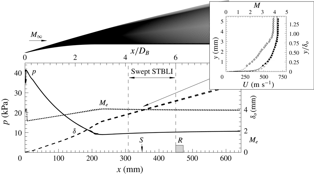
The base model (ogive-cylinder body) was designed with the aim of establishing a simplified geometry, to produce a fully turbulent axisymmetric base flow, and serving as a common reference across the programme. As shown in figure 2, the numerical domain models the flow close ahead of the nose leading-edge shock and extends down to
 $x=0.64$
m over the cylindrical section (
 $8.5D_{B}$
). Computational simulations used a Reynolds-averaged Navier–Stokes numerical procedure with the Baldwin–Lomax turbulence model (see Chandola et al.
Reference Chandola, Huang and Estruch-Samper2017). Experimental boundary-layer profiles of velocity and Mach number were also obtained through Pitot tube measurements (taken at the mean separation location for the reference axisymmetric case,
 $x=336$
mm), yielding a turbulent profile in close agreement with the simulations. As shown in the numerical estimates, the boundary layer grows from
 $\unicode[STIX]{x1D6FF}_{o}=3.9$
mm at the present upstream separation location,
 $x_{o}=349$
mm (with local conditions as per table 1, used as a common reference), to 4.5 mm by the location where the obstacle leading edge is later placed,
 $x_{S}=450$
mm, with boundary-layer edge at
 $99.5\,\%\,U_{e}$
. At this high Reynolds number, the boundary layer is developed to a fully turbulent state and is practically at equilibrium, maintaining a shape factor
 $H=1.41\pm 0.02$
and with minimal pressure and Mach-number gradients over the measurement range.
Reference base flow (undisturbed, without obstacle) over ogive-cylinder body: schematic of numerical domain and respective estimates of pressure
 $p$
(solid line, left axis), edge Mach number
 $M_{e}$
(dotted line, right axis) and boundary-layer thickness
 $\unicode[STIX]{x1D6FF}_{o}$
(dashed line, right axis). Based on turbulent CFD (
 $N_{x}\times N_{y}=1301\times 1500$
,
 $y^{+}=1$
for fine resolution mesh in black;
 $N_{x}\times N_{y}=323\times 374$
,
 $y^{+}=4$
for coarse mesh in grey). Boundary-layer profiles of velocity
 $U$
(black squares) and Mach number
 $M$
(grey diamonds) are compared with experimental measurements taken close ahead of separation, as per Estruch-Samper & Chandola (Reference Estruch-Samper and Chandola2018). Free-stream flow conditions are
 $M_{\infty }=3.93$
,
 $Re_{\infty }=7.0\times 10^{7}~\text{m}^{-1}$
; sample domain shown on top.

2.2 Mean flow organisation
The mean pressure results along the interaction are presented in figure 3(a–c), where
 $X=x-x_{o}$
is shown with respect to the upstream separation location at
 $\unicode[STIX]{x1D711}=0^{\circ }$
(table 1). The axial pressure gradient upon separation,
 $\text{d}p/\text{d}x$
, is first seen to follow the same tendency as in the reference case near
 $\unicode[STIX]{x1D711}=0{-}30^{\circ }$
, to then undergo a slight expansion associated with a localised flow deflection closer to the corner, markedly within the reference range, and followed by a further overshoot just ahead of the obstacle – as often encountered for moderately swept interactions, e.g. analogous to the blunt-fin interactions in Brusniak & Dolling (Reference Brusniak and Dolling1994). The normalised pressure gradient
 $\unicode[STIX]{x1D6FD}=\unicode[STIX]{x1D6FF}^{\ast }/\unicode[STIX]{x1D70F}_{w}(\text{d}p/\text{d}x)$
at separation (as per Laderman Reference Laderman1980) is found to drop slightly as the local pressure gradient across the shock is moderately reduced and sweep angle is progressively increased from
 $\unicode[STIX]{x1D6EC}=0^{\circ }$
to
 $30^{\circ }$
within the swept separation range (
 $\unicode[STIX]{x1D711}=25^{\circ }$
–
 $135^{\circ }$
), with displacement thickness
 $\unicode[STIX]{x1D6FF}^{\ast }=1.9$
mm and wall shear stress
 $\unicode[STIX]{x1D70F}_{w}=105$
Pa estimated from CFD. The scale of separation follows a similar tendency, as compared with (
 $90^{\circ }-\unicode[STIX]{x1D6EC}$
), varying from
 $L/\unicode[STIX]{x1D6FF}_{o}=26$
to 18 within the region of interest (
 $\unicode[STIX]{x1D711}<135^{\circ }$
), with obstacle height falling
 $h<\unicode[STIX]{x1D6FF}_{o}$
thereafter. The interaction thus overall lies within the moderately swept separation regime, whereby
 $\unicode[STIX]{x1D6EC}<30^{\circ }$
, rendering it more closely comparable to cylindrically symmetric swept configurations (e.g. as expected for high-deflection, blunt geometries).
Mean flow organisation: (a) streamwise variation in wall pressure at different azimuthal planes, (b) azimuthal variation in separation scale
 $L/\unicode[STIX]{x1D6FF}_{o}$
, sweep angle
 $\unicode[STIX]{x1D6EC}$
and normalised axial pressure gradient
 $\unicode[STIX]{x1D6FD}=\unicode[STIX]{x1D6FF}^{\ast }/\unicode[STIX]{x1D70F}_{w}(\text{d}p/\text{d}x)$
, and (c) pressure contour in the
 $(X,\unicode[STIX]{x1D711})$
plane, at
 $(\unicode[STIX]{x0394}X,\unicode[STIX]{x0394}\unicode[STIX]{x1D711})=(4.5~\text{mm},6.5~\text{mm})$
resolution, where
 $\unicode[STIX]{x0394}\unicode[STIX]{x1D711}=10^{\circ }$
. Reference axisymmetric case (
 $L/\unicode[STIX]{x1D6FF}_{o}\approx 30$
) offset closer to the obstacle to match separation location for the present
 $x_{o}=-26\unicode[STIX]{x1D6FF}_{o}$
, at
 $\unicode[STIX]{x1D711}=0^{\circ }$
.

Sample time-dependent pressure along separation region and near reattachment, at planes
 $\unicode[STIX]{x1D711}=0^{\circ }$
and spanning over durations of: (a)
 $tU_{e}/\unicode[STIX]{x1D6FF}_{o}=50\,000$
, (b)
 $tU_{e}/\unicode[STIX]{x1D6FF}_{o}=25\,000$
, (c)
 $tU_{e}/\unicode[STIX]{x1D6FF}_{o}=12\,500$
and (d)
 $tU_{e}/\unicode[STIX]{x1D6FF}_{o}=6250$
. Plots correspond to the same sample and progressively narrow down towards a period equivalent to
 ${\sim}25T_{o}$
(d). Signal near reattachment
 ${\sim}x_{R}$
corresponds to the measurement station just ahead of the obstacle and separation location
 $x_{o}$
is determined based on the local
 $\bar{p}/\unicode[STIX]{x1D70E}_{p}$
maximum, where
 $\bar{p}$
is mean pressure (simplified to
 $p$
throughout the text) and
 $\unicode[STIX]{x1D70E}_{p}$
is standard deviation. Reference pressure corresponds to the undisturbed level of
 $p_{u}=9.84$
kPa near separation (as obtained for the base body only, without the obstacle).

Time-dependent pressure over sample periods of 25 ms duration and respective pressure contours in the
 $(t,x)$
plane at: (a) reference plane
 $\unicode[STIX]{x1D711}=0^{\circ }$
, (b)
 $\unicode[STIX]{x1D711}=30^{\circ }$
, (c)
 $\unicode[STIX]{x1D711}=60^{\circ }$
, (d)
 $\unicode[STIX]{x1D711}=90^{\circ }$
, (e)
 $\unicode[STIX]{x1D711}=120^{\circ }$
and (f)
 $\unicode[STIX]{x1D711}=150^{\circ }$
. Dashed lines indicate the local separation location
 $x_{o}$
, at each respective plane and the
 $5\unicode[STIX]{x1D6FF}_{o}$
location downstream,
 ${\sim}(0.5L_{i}+2\unicode[STIX]{x1D6FF}_{o})$
, at shear-layer inception.

3 Interaction unsteadiness
3.1 Time-resolved wall pressure
Surface pressure measurements mapped the azimuthal
 $\unicode[STIX]{x1D711}=0^{\circ }{-}180^{\circ }$
range, over
 $-1.25L_{o}<x<x_{S}$
, with separation length at the reference plane
 $L_{o}=101.3$
mm. Samples of the time-dependent pressure traces near the separation location
 $x_{o}$
over the same plane (
 $\unicode[STIX]{x1D711}=0^{\circ }$
) are presented in figure 4. A duration of
 $tU_{e}/\unicode[STIX]{x1D6FF}_{o}=50\,000$
(
 $t=285.5$
ms) is first shown, corresponding to approximately
 ${\sim}$
5 % of the total signal in the subsequent spectral analysis – which considers durations of order
 $tU_{e}/\unicode[STIX]{x1D6FF}_{o}\approx 10^{6}$
– and where the highly unsteady nature of the flow may be noted. Closer insights are then obtained as the same samples are presented over progressively shorter durations of
 $tU_{e}/\unicode[STIX]{x1D6FF}_{o}=25\,000$
and 12 500. As the range is further narrowed to
 $tU_{e}/\unicode[STIX]{x1D6FF}_{o}=6250$
(35.7 ms), the larger-amplitude fluctuations become better defined, with the shock oscillations near separation being more clearly distinguished. The local pressure near separation may be seen to oscillate between the lower reference (undisturbed) pressure ahead of the interaction
 $p_{u}=9.84$
kPa and the plateau levels
 $p_{p}\approx 28$
kPa (
 ${\sim}2.85p_{u}$
) in a relatively periodic fashion. The pressure near reattachment
 ${\sim}x_{R}$
, as measured just ahead of the obstacle, in turn oscillates between the plateau and values as high as
 ${\sim}7p_{u}$
, where the high reattachment angle leads to a detached shock wave, with fluctuations being out of phase with respect to those at separation. As per the preceding phases of the programme, the varying levels of correlation between shock motions and the higher-frequency disturbances along the separation region are characterised by in-phase/anti-phase switches, similar to those observed for incident-shock interactions in the LES studies by Agostini, Larchevêque & Dupont (Reference Agostini, Larchevêque and Dupont2015).
Figure 5 goes on to present samples of the time-dependent pressure over different azimuthal planes and alongside their respective contours, comprising the combined simultaneous measurements over the
 $(t,x)$
domain for each
 $\unicode[STIX]{x1D711}$
plane. Results cover a duration of 25 ms each (
 $tU_{e}/\unicode[STIX]{x1D6FF}_{o}=4500$
), resolving in further detail the low-frequency dynamics of separation shock pulsations – with fluctuation levels primarily found at low frequencies over the intermittency length
 $L_{i}$
, defined as the range over which the shock foot oscillates and where the larger-amplitude fluctuations are inherently induced. Upon first assessment, oscillations may hence be noted to increase in frequency at azimuthal locations farther from the reference plane
 $\unicode[STIX]{x1D711}=0^{\circ }$
and smaller-amplitude/high-frequency fluctuations are found within the recirculation region, sufficiently far from separation and reattachment. Similar tendencies are then observed as the separation shock is progressively swept, with slightly reduced pressure levels at locations farther from the reference plane (figure 3
c). Further insights are next to be drawn through spectral analysis of the signals, with sensor response safely enabling interpretation up to
 ${\sim}$
50 kHz.
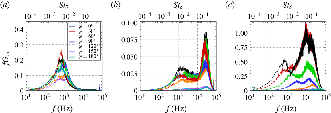
Pressure PSD along reference plane,
 $\unicode[STIX]{x1D711}=0^{\circ }$
: (a) near separation and pressure rise, (b) early shear-layer development, (c) shear-layer evolution and (d) close ahead of the obstacle. The corresponding schlieren image highlights the shear-layer development upon separation.

Streamwise variation in pressure PSD over different azimuthal planes: (a) at reference plane
 $\unicode[STIX]{x1D711}=0^{\circ }$
, (b)
 $\unicode[STIX]{x1D711}=30^{\circ }$
, (c)
 $\unicode[STIX]{x1D711}=60^{\circ }$
, (d)
 $\unicode[STIX]{x1D711}=90^{\circ }$
, (e)
 $\unicode[STIX]{x1D711}=120^{\circ }$
and (f)
 $\unicode[STIX]{x1D711}=150^{\circ }$
; with respective schlieren images. Arrows indicate shift to lower frequencies as the shear layer evolves along the separation region.

3.2 Spectral characterisation
The pressure power spectral density (PSD) along the reference plane
 $\unicode[STIX]{x1D711}=0^{\circ }$
is presented in its premultiplied form
 $fG_{xx}$
in figure 6, where axial locations are shown normalised with respect to the reference separation length, as
 $X^{\ast }=X/L_{o}$
. A strong low-frequency dominance is found near separation, with the local maxima at 719 Hz – a Strouhal number
 $St_{L}=fL_{o}/U_{b}$
of 0.11 with reference to velocity behind the separation shock
 $U_{b}=638~\text{m}~\text{s}^{-1}$
(outer shear-layer edge), as based on the measured pressure rise across separation and upstream Mach number,
 $p_{p}/p_{u}=2.85$
and
 $M_{e}=3.92$
. This is then followed by the emergence of high-frequency fluctuations at
 ${\sim}$
37 kHz (
 $St_{L}=5.9$
), associated with the incipient instability of the separated shear layer close downstream of separation, as indicated in the
 $(t,x)$
contours from figure 5 as well. Thereafter, the shear layer’s shedding is seen to shift to lower frequencies – through Kelvin–Helmholtz (KH) instability – as it evolves along the recirculation length, here attaining 8.8 kHz (
 $St_{L}\approx 1.4$
) close ahead of the obstacle. To enable interpretation with reference to the boundary-layer time scales, the top axis in the spectra is shown in terms of
 $St_{\unicode[STIX]{x1D6FF}}=f\unicode[STIX]{x1D6FF}_{o}/U_{b}$
, where the respective Strouhal numbers are seen to shift from approximately
 $St_{\unicode[STIX]{x1D6FF}}=0.21$
at inception to
 $St_{\unicode[STIX]{x1D6FF}}=0.05$
near the obstacle (both at
 $\unicode[STIX]{x1D711}=0^{\circ }$
). The low-frequency dominance associated with separation bubble pulsations is again encountered near reattachment, superimposed on the higher local shear-layer perturbation levels.
The spectral evolutions at other azimuthal locations over the swept separation zone are further presented in figure 7, where the shear-layer spectra are found to exhibit a similar tendency across the different azimuthal planes. The formation of the separated shear layer is further evidenced in the schlieren images across all planes, consistently seen to extend towards the obstacle’s upper edge, leaving the separation region close ahead of it (see the respective stages of shear-layer evolution in figure 6). As further evaluated through the point-to-point coherence
 $C_{x,1-x}$
(at
 $\unicode[STIX]{x0394}x=-1.15\unicode[STIX]{x1D6FF}_{o}$
) in figure 8, eddy structures remain well defined, with relatively high coherence as they evolve along the recirculation length – their growth being in turn inherently sustained via the entrainment of the surrounding flow and hence partly feeding from the separation, as further laid out in § 4.
Streamwise variation in point-to-point coherence
 $C_{x,1-x}$
: (a) at reference plane
 $\unicode[STIX]{x1D711}=0^{\circ }$
, (b)
 $\unicode[STIX]{x1D711}=30^{\circ }$
, (c)
 $\unicode[STIX]{x1D711}=60^{\circ }$
, (d)
 $\unicode[STIX]{x1D711}=90^{\circ }$
, (e)
 $\unicode[STIX]{x1D711}=120^{\circ }$
and (f)
 $\unicode[STIX]{x1D711}=150^{\circ }$
. Arrows indicate shift to lower frequencies as the shear layer evolves along the separation region. Line legend as per figure 7.

Contours of pressure PSD in the
 $(f,x)$
plane comprising the overall spectra at azimuthal planes: (a)
 $\unicode[STIX]{x1D711}=0^{\circ }$
, (b)
 $\unicode[STIX]{x1D711}=30^{\circ }$
, (c)
 $\unicode[STIX]{x1D711}=60^{\circ }$
, (d)
 $\unicode[STIX]{x1D711}=90^{\circ }$
, (e)
 $\unicode[STIX]{x1D711}=120^{\circ }$
and (f)
 $\unicode[STIX]{x1D711}=150^{\circ }$
. Together with (g) schematic in the form of a three-dimensional pressure contour over the complete perimeter (symmetry at
 $\unicode[STIX]{x1D711}=0^{\circ }$
), indicating respective location for each azimuthal plane.

Combined plot of PSD spectra over azimuthal direction and taken at: (a) local separation
 $x_{o}$
line, (b) shear-layer inception
 $x_{i}$
line, and (c) shear-layer ejection
 $x_{ej}$
line, close ahead of the obstacle. Panels correspond to the respective locations within each azimuthal plane.

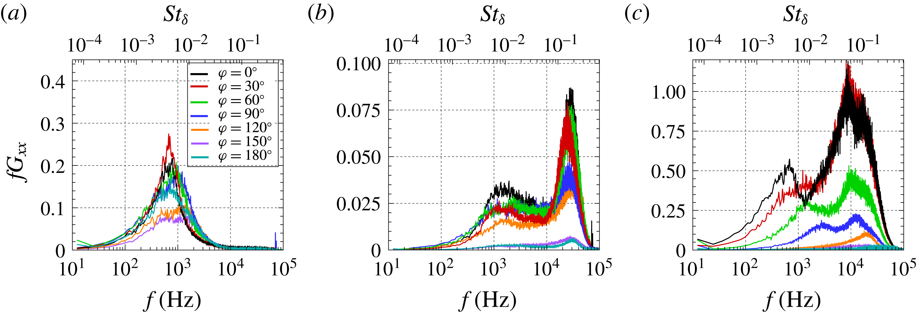
Azimuthal variation in pressure PSD at: (a) local separation location
 $x_{o}$
, (b) shear-layer inception
 $x_{i}$
, and (c) close ahead of the obstacle, where the shear layer is ejected
 $x_{ej}$
. Panels correspond to selected planes within the contours in figure 10.
Figures 9(a–f) present the contour maps composed of the PSD of all the signals over the complete axial measurement length, with the streamwise evolution of premultiplied spectral content in the
 $(f,x)$
plane, and at different azimuthal locations indicated in the accompanying pressure contour (in figure 9
g). The spectra further reflect the dominant influence of the separated shear layer, which is seen to emerge close downstream of the mean separation location – evidenced close behind the shock’s oscillation range – and then remains well defined within
 $\unicode[STIX]{x1D711}=0^{\circ }$
–
 $120^{\circ }$
(
 $\unicode[STIX]{x1D6EC}\leqslant 30^{\circ }$
). The dominant low-frequency unsteadiness near separation
 $f_{o}$
, of order
 $10^{2}{-}10^{3}$
Hz, is again clearly observed throughout the interaction’s span, localised along the separation shock’s foot, with notable (yet broadband) low-frequency levels found near reattachment as well.
As such, results reflect the dominance of shear-layer perturbation levels, induced as large eddies convect along the bubble at supersonic convection velocity – where the bounding Mach numbers on the outer/inner sides of the shear layer are respectively that behind the shock
 $M_{b}$
(table 1) and
 $M\approx 0.05$
(near the stagnation line). As per the schlieren in figure 7, fluctuations are attributed to acoustic disturbances radiated by eddies as they evolve along the recirculation, yet their precise modulation as they propagate across the reverse flow – towards the wall – appears challenging to establish. Evidence of similar acoustic disturbances is for instance found in past studies by Papamoschou (Reference Papamoschou1995) on counterflow supersonic mixing layers, where they were noted to emanate normally to turbulent eddy structures and subsequently weakened into Mach waves a short distance away. Under the subsonic reverse flow conditions in the present case (cf. the supersonic counterflows in the above), the latter stage of shocklet mitigation is thus bound to be significantly delayed, with perturbations here expected to maintain most of their strength by the time they reach the wall. From the present spectra (e.g. in figures 6 and 7), it may be further noted that disturbances are radiated with strong streamwise directivity, as levels are cumulatively enhanced towards the obstacle, with negligible upstream propagation.
Figure 10 presents the combined PSD of the signals over the complete azimuthal range and at selected locations, accordingly taken at (tracing) the local separation line
 $x_{o}$
, at shear-layer inception
 $x_{i}$
and upon its ejection
 $x_{ej}$
close ahead of the obstacle, with the respective contour maps (essentially a planform view of the plots) shown to further highlight the order-of-magnitude differences in perturbation levels. The unsteadiness at separation
 $f_{o}$
is noted to be practically associated in full with shock pulsations of order
 $O(10^{2}{-}10^{3})$
Hz, without a trace of higher-frequency shear-layer levels at that stage. Close downstream of the separation line, as shear-layer fluctuations emerge, perturbations exhibit the highest frequencies along the interaction (here referred to as shear-layer inception frequencies
 $f_{i}$
) while thereafter, at the ejection location (taken close ahead of the obstacle), frequency levels
 $f_{ej}$
instead progressively decrease at locations farther from the upstream separation plane, towards higher
 $\unicode[STIX]{x1D711}$
planes. For closer comparison, the respective spectral profiles at different azimuthal planes are shown overlapped in figure 11, where the tendency towards higher ejection frequencies is more clearly evidenced, and with the levels upon inception noted to be significantly higher along the
 $\unicode[STIX]{x1D711}=0^{\circ }{-}120^{\circ }$
range (
 $\unicode[STIX]{x1D6EC}\leqslant 30^{\circ }$
). As per our earlier studies, the inception frequencies appear to remain at approximately
 ${\sim}0.2U_{e}/\unicode[STIX]{x1D6FF}_{o}$
, independently of the local scale of separation and related downstream conditions.
Streamwise evolution in: (a) characteristic frequency
 $f_{ch}$
, (b) phase velocity
 $v_{\unicode[STIX]{x1D719}}$
and (c) associated wavelength
 $\unicode[STIX]{x1D706}_{w}$
. Plots for different azimuthal planes (left column) and respective contours (right column), at
 $(\unicode[STIX]{x0394}X,\unicode[STIX]{x0394}\unicode[STIX]{x1D711})=(4.5~\text{mm},6.5~\text{mm})$
resolution, where
 $\unicode[STIX]{x0394}\unicode[STIX]{x1D711}=10^{\circ }$
. Results map the complete STBLI region, with incoming boundary-layer characteristic frequencies falling outside sensor frequency response (
 ${\gtrsim}50$
kHz) and of order
 $U_{e}/\unicode[STIX]{x1D6FF}_{o}\approx 180$
kHz. Dark grey symbols indicate the respective values for the reference axisymmetric step case (
 $h_{ref}=22.5$
mm).

3.3 Swept separated shear layer
The shear-layer kinematics over the same axial planes are subsequently assessed in figure 12 in terms of the streamwise evolution of characteristic frequency
 $f_{ch}$
, corresponding to the maxima extracted from the premultiplied spectra
 $fG_{xx}$
, together with phase velocity
 $v_{\unicode[STIX]{x1D719}}=2\unicode[STIX]{x03C0}f\unicode[STIX]{x1D709}/\unicode[STIX]{x1D719}$
and the associated wavelength
 $\unicode[STIX]{x1D706}_{w}=v_{\unicode[STIX]{x1D719}}/f_{ch}$
, where
 $\unicode[STIX]{x1D719}$
is the phase deduced from the cross-spectra between adjacent sensor locations and
 $\unicode[STIX]{x1D709}$
is sensor spacing (see § 2). Along the swept separation range,
 $f_{ch}$
is found to decrease monotonically all the way towards the obstacle, where the shear layer leaves the separation. It is at this location – at the point where the local shedding appears to settle closer to the obstacle – where the mass entrained within eddies is deemed to be ejected, depleting that mass away from the bubble. As earlier noted, the frequencies upon ejection accordingly attain lower levels near the reference plane and increase over the
 $\unicode[STIX]{x1D711}$
direction, while the maximum frequencies correspond to the incipient shear-layer instability
 $f_{i}$
downstream of separation and with a moderate reduction approximately from
 $f_{i}=37$
kHz to 30 kHz. This proves once again consistent with the observations in Estruch-Samper & Chandola (Reference Estruch-Samper and Chandola2018), where shear-layer growth was established to be largely unaffected by the scale of separation but noted to be instead primarily driven by local flow conditions (
 $p_{u}$
,
 $M_{e}$
,
 $\unicode[STIX]{x1D6FF}_{o}$
). The phase velocity
 $v_{\unicode[STIX]{x1D719}}$
is in turn also noted to decrease to some extent in the axial direction over the reference plane
 $\unicode[STIX]{x1D711}=0^{\circ }$
, from approximately
 $0.58U_{b}$
to
 $0.42U_{b}$
, given the asymmetric nature of the separated shear layer, and meeting symmetry levels (
 ${\sim}0.5U_{b}$
) near the middle of the recirculation, with lower bound practically near the stagnation line. The phase velocity
 $v_{\unicode[STIX]{x1D719}}$
then increases with
 $\unicode[STIX]{x1D711}$
over the swept range – with growing sweep angle
 $\unicode[STIX]{x1D6EC}$
, in turn resulting in a locally higher
 $M_{c}$
(given the slightly reduced shock strength, as per figure 3
b). The associated wavelength
 $\unicode[STIX]{x1D706}_{w}$
grows monotonically towards the obstacle, starting at approximately
 $\unicode[STIX]{x1D706}_{w}/\unicode[STIX]{x1D6FF}_{o}\approx 2$
and attaining larger scales upon ejection at planes near
 $\unicode[STIX]{x1D711}=0^{\circ }$
, where the shear layer develops over a longer path, to then decrease gradually over the swept separation zone.
Unsteadiness of swept STBLI: (a) characteristic frequency
 $f_{ch}$
contour over the
 $(X,\unicode[STIX]{x1D711})$
domain, and azimuthal correlation along reattachment plane (
 ${\sim}x_{ej}$
): (b)
 $\unicode[STIX]{x1D711}=10{-}50^{\circ }$
with respect to
 $\unicode[STIX]{x1D711}=0^{\circ }$
, (c)
 $\unicode[STIX]{x1D711}=60{-}90^{\circ }$
with respect to
 $\unicode[STIX]{x1D711}=50^{\circ }$
, and (d)
 $\unicode[STIX]{x1D711}=100{-}130^{\circ }$
with respect to
 $\unicode[STIX]{x1D711}=90^{\circ }$
. Cross-correlations apply signal low-pass filtering at 2 kHz to assess low-frequency effects (note no pre-filtering is applied in the remaining results unless specifically indicated).

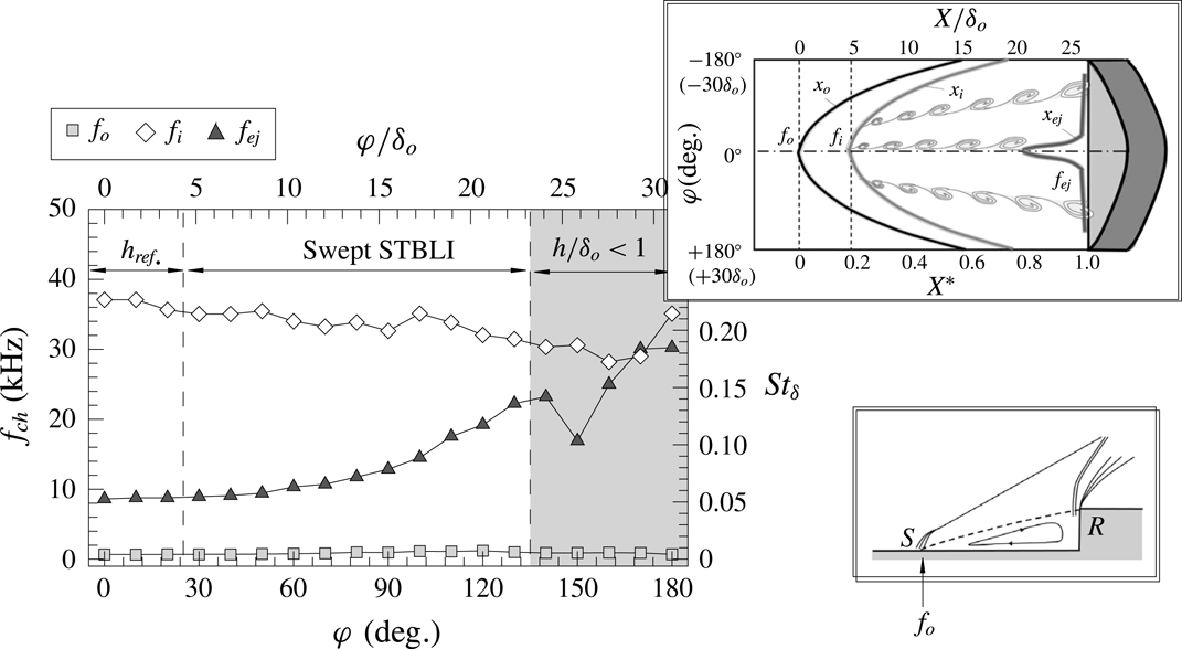
Azimuthal variation in characteristic frequencies
 $f_{ch}$
over the complete azimuthal range, with schematic representing the variation in the following three locations over the
 $(X,\unicode[STIX]{x1D711})$
domain: dominant low-frequency unsteadiness near separation
 $f_{o}$
, high-frequency unsteadiness upon shear-layer inception
 $f_{i}$
and frequency upon ejection
 $f_{ej}$
.

The shear layer’s evolution is further captured in figure 13(a), which maps the azimuthal change in characteristic frequency
 $f_{ch}$
over the complete
 $(X,\unicode[STIX]{x1D711})$
domain, highlighting the three-dimensional variation in its shedding rates, together with the dominant low-frequency unsteadiness over the swept separation range; note also the resulting sharp rise, of nearly two orders of magnitude, from separation to inception. Details on the azimuthal cross-correlations along the reattachment plane
 $\unicode[STIX]{x1D70C}_{ox}$
in figure 13(b–d) (low-pass filtered at
 $2\times 10^{3}$
Hz to isolate the local low-frequency effects) are further presented to assess the level of spanwise correlation at this salient location. For this purpose, alternative instrumentation arrangements were used, with four rows of eight sensors distributed over the base cylinder perimeter at a spacing
 $\unicode[STIX]{x0394}\unicode[STIX]{x1D711}=10^{\circ }$
(6.5 mm) and matching the same axial locations through combined configurations, the data herein corresponding to the row just ahead of the step,
 ${\sim}x_{ej}$
. While noting the absence of clear integral length scales, given that local instabilities are primarily imposed by the swept shear-layer properties upon ejection (as per the captured
 $f_{ch}$
tendencies), the azimuthal measurements evidence that the local shock structure exhibits an oscillating behaviour, where negative delays (
 $\unicode[STIX]{x0394}\unicode[STIX]{x1D70F}<0$
) in the spanwise propagation of disturbances indicate an earlier response of the signal at the given reference plane – whereby the local pulsation rate is lower, closer to the upstream separation plane (more details in § 4) – and with the level of correlation accordingly decreasing towards farther planes, with respect to the given references. As further evidenced next, this pulsating behaviour is remarked to be characterised by a gradual variation in pulsation frequency, as the flow is swept farther from
 $\unicode[STIX]{x1D711}=0^{\circ }$
.
Having documented the shear layer’s evolution, the variation in the characteristic frequencies at separation
 $f_{o}$
, shear-layer inception
 $f_{i}$
and upon ejection
 $f_{ej}$
go on to be more closely assessed in figure 14. The instability of the bubble at separation – in essence capturing the large-amplitude fluctuations attributed to shock pulsations – is found to exhibit relatively lower frequencies (
 $St_{\unicode[STIX]{x1D6FF}}\approx 0.004$
–0.008, within one to two orders of magnitude lower than those near inception and ejection). Instead, the characteristic frequencies at inception drop progressively as the boundary layer grows from
 $\unicode[STIX]{x1D6FF}_{o}=3.9$
mm to 4.3 mm (locally upon separation), remaining within
 ${\sim}0.2U_{e}/\unicode[STIX]{x1D6FF}_{o}$
. Thereafter, the dominant frequency upon ejection
 $f_{ej}$
exhibits a marked increasing tendency over the azimuthal direction, within the swept separation range, at approximately
 $St_{\unicode[STIX]{x1D6FF}}\approx 0.05$
–0.21. As per the evolutions in figure 12(a), it may thus be corroborated that the variations in the latter are in great part determined by the shorter extent of separation – i.e. local separation
 $L$
, and hence shear-layer length – which in essence leads to lower frequencies being attained upon ejection for longer development paths. As such, while higher ejection frequencies are attained farther from the reference plane, the scale of eddies is in turn accordingly smaller, counteracting their local entrainment capabilities (along their way towards, and up to, ejection) within a given streamwise path.
Azimuthal variation in low-frequency unsteadiness
 $f_{o}$
, along separation shock foot. Horizontal line marks the level of low-frequency unsteadiness for the reference highly separated case (axisymmetric
 $h=22.5$
mm step, with
 $f_{o}=391$
Hz). The density ratio across the shear layer is estimated to vary from
 $s=0.33$
to 0.30 farther from
 $\unicode[STIX]{x1D711}=0^{\circ }$
(as Mach number behind the shock increases
 $M_{b}=3.16$
–3.44) rendering
 $\unicode[STIX]{x1D6FF}^{\prime }$
variations negligible along the interaction’s span.

4 Low-frequency breathing of swept separation
4.1 Separation shock unsteadiness
The azimuthal variation in low-frequency unsteadiness is more closely assessed in figure 15, where the progressive increase in
 $f_{o}$
at locations farther from the reference plane is clearly observed, as the local separation scale is shortened towards
 $\unicode[STIX]{x1D711}\rightarrow 120^{\circ }$
. In this instance, the tendency in low-frequency unsteadiness appears in fact opposed to the decrease in
 $f_{o}$
reported along the separation line in a number of swept STBLI studies in the literature – mostly on highly swept configurations where both the separation and reattachment, and hence the ejection location
 $x_{ej}$
, are gradually displaced downstream (as per § 1, see the noted reviews for details on common variations in mean flow organisation amongst swept interactions). This is expected to differ here, within
 $\unicode[STIX]{x1D711}\leqslant 120^{\circ }$
, given that reattachment is close to the obstacle’s upper edge. As further indicated in figure 15, the low-frequency unsteadiness in the present interaction remains well above that documented for the reference axisymmetric case at the same flow conditions (
 $f_{o}=391$
Hz,
 $St_{\unicode[STIX]{x1D6FF}}=0.0023$
), with separation length
 $L/\unicode[STIX]{x1D6FF}_{o}=30$
, this being nearly twice lower than the frequencies within the present reference plane (
 $f_{o}=719$
Hz,
 $St_{\unicode[STIX]{x1D6FF}}=0.0044$
). Results therefore confirm that relatively higher pulsation frequencies may be expected in swept STBLIs, as evidenced here through comparison with its analogue axisymmetric case. Of particular interest is the fact that the swept bubble does not pulsate at a ‘global’ breathing frequency, but instead the low-frequency unsteadiness varies progressively over the spanwise direction (see figure 15). These tendencies are hereby argued to be intrinsically associated with the bubble breathing mechanism; as such, the shear layer’s influence on interaction unsteadiness is examined in closer detail next.
4.2 Shear-layer entrainment and mass ejection
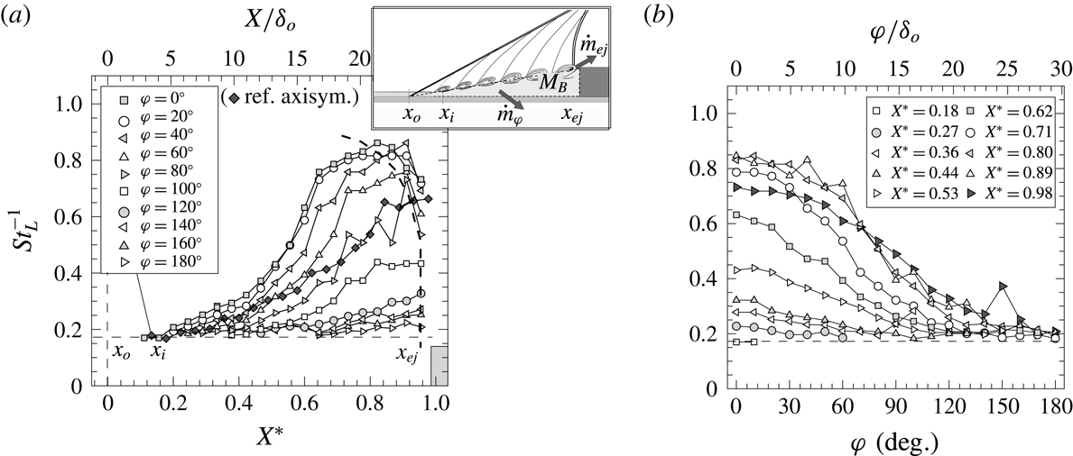
Shear-layer evolution in terms of inverse of Strouhal number based on local (axial) separation length
 $St_{L}^{-1}$
, respectively over: (a) streamwise
 $X^{\ast }$
and (b) azimuthal directions
 $\unicode[STIX]{x1D711}$
. Schematic represents shear-layer inception location (
 $x_{i}$
) close downstream of separation
 $x_{o}$
and rate of mass entrainment
 ${\dot{m}}_{ej}$
close ahead of the obstacle
 $x_{ej}$
. Streamwise evolution for reference axisymmetric test case (black diamonds) indicated for comparison.

The scale of separation is thus seen to effectively determine the shear layer’s development length along the recirculation and in turn dictates the local ejection frequencies
 $f_{ej}$
at different spanwise locations (within the ejection plane), where shear-layer spreading rate
 $\unicode[STIX]{x1D6FF}^{\prime }$
is in great part dictated by its convection Mach number and the velocity and density gradients across it. This is broadly in accordance with the views in the preceding phase of the present programme (§ 1), herein evaluated for the case of swept interactions.
As per Dupont et al. (Reference Dupont, Haddad and Debiève2006), we may therefore characterise the shear-layer growth through a
 $St_{L}/X^{\ast -1}$
scaling – effectively equivalent to
 $(U_{c}/U_{b})(S_{tr}/\unicode[STIX]{x1D6FF}^{\prime })$
, where
 $S_{tr}=f\unicode[STIX]{x1D6FF}_{\unicode[STIX]{x1D714}}/U_{c}$
is the classical Strouhal number for a mixing layer with convection velocity
 $U_{c}$
and thickness
 $\unicode[STIX]{x1D6FF}_{\unicode[STIX]{x1D714}}=\unicode[STIX]{x1D6FF}^{\prime }X$
. As such, figure 16(a) presents
 $St_{L}^{-1}$
over the normalised axial length to factor in the shear layer’s evolution. The shift from high to mid frequencies as the shear layer evolves across different azimuthal planes therefore leads to an increasing tendency in
 $St_{L}^{-1}$
, with lower levels upon ejection at locations farther from
 $\unicode[STIX]{x1D711}=0^{\circ }$
(as higher values of
 $f_{ej}$
are attained). Comparison with the analogue axisymmetric case for the reference large-scale separation at the same incoming conditions finds the shift to lower frequencies accelerated within
 $\unicode[STIX]{x1D711}=0^{\circ }$
–
 $90^{\circ }$
, closer to the upstream separation region, but to then diminish at farther planes, as the shock is increasingly swept (
 $\unicode[STIX]{x1D6EC}\geqslant 15^{\circ }$
). To further document the respective variations over the spanwise direction, figure 16(b) presents the corresponding azimuthal trends. While the precise streamwise direction of the large convecting structures is challenging to determine, this may be here estimated based on the given correlations.
Figure 17(a) goes on to evaluate the axial shear-layer evolution by comparing the
 $St_{L}/X^{\ast -1}$
slope against the variation in low-frequency unsteadiness, normalised as a function of the reference boundary-layer thickness
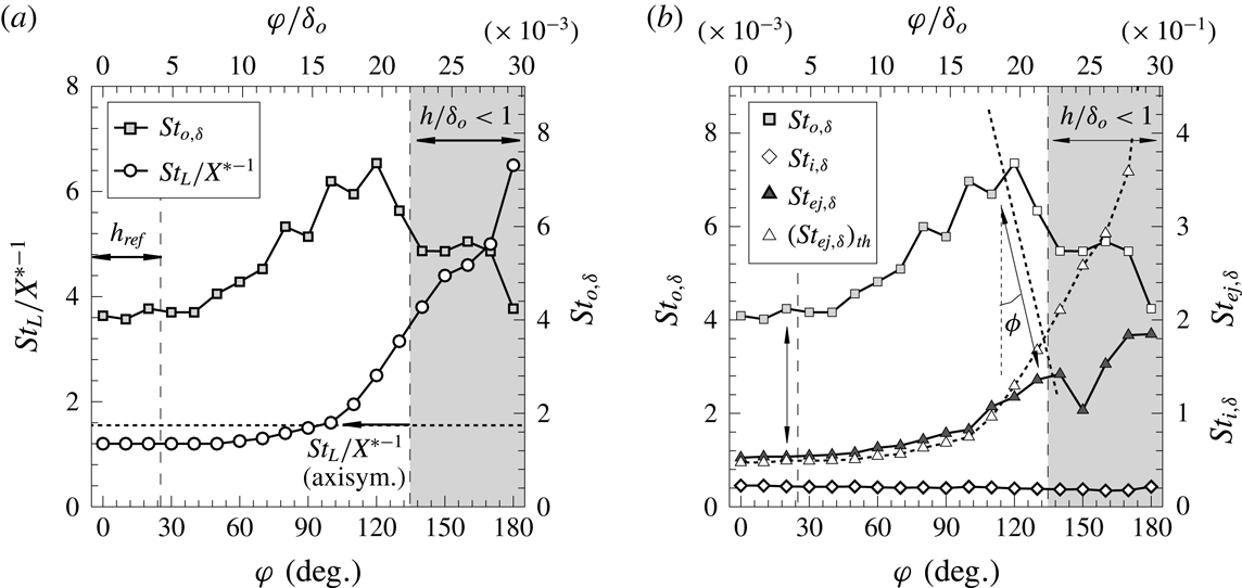
 $St_{o,\unicode[STIX]{x1D6FF}}(=f_{o}\unicode[STIX]{x1D6FF}_{o}/U_{b})$
, where both quantities are found to exhibit a similar increasing tendency over the azimuthal direction. The shear-layer growth is seen to start at slightly greater slopes compared to the reference axisymmetric case, i.e with enhanced spreading, and then keeps decreasing towards the higher
 $\unicode[STIX]{x1D711}$
planes (as local gradients across it vary), attaining similar levels by
 $\unicode[STIX]{x1D711}\approx 90^{\circ }$
. As further shown in figure 17(b), the same tendency is noted for the Strouhal number upon ejection
 $St_{ej,\unicode[STIX]{x1D6FF}}~(=f_{ej}\unicode[STIX]{x1D6FF}_{o}/U_{b})$
, this being also compared to the respective theoretical estimate, which as per figure 12(a) and consistently with our latter studies may be taken to scale as
 $$\begin{eqnarray}St_{ej,\unicode[STIX]{x1D6FF}}^{-1}\approx St_{i,\unicode[STIX]{x1D6FF}}^{-1}+\frac{1}{St_{L}/X^{\ast -1}}\left(\frac{L}{\unicode[STIX]{x1D6FF}_{o}}\right)X_{ej}^{\ast },\end{eqnarray}$$
that is, as a function of the shear layer’s growth since its inception and up to the relative ejection location,
 $X_{ej}^{\ast }=(x-x_{o})/L$
.
Evaluation of azimuthal variation in low-frequency unsteadiness
 $St_{o,\unicode[STIX]{x1D6FF}}$
: (a) comparison with shear-layer growth characterised by
 $St_{L}/X^{\ast -1}$
slope and (b) with frequency at shear-layer inception and at ejection,
 $St_{i,\unicode[STIX]{x1D6FF}}$
and
 $St_{ej,\unicode[STIX]{x1D6FF}}$
, together with theoretical estimate for the latter
 $(St_{ej,\unicode[STIX]{x1D6FF}})_{th}$
as per equation (4.1). The horizontal line marks the
 $St_{L}/X^{\ast -1}=1.55$
threshold for the reference highly separated case (axisymmetric
 $h=22.5$
mm step);
 $\unicode[STIX]{x1D719}$
indicates the estimated spanwise flow deflection angle with reference to separation (
 $\unicode[STIX]{x0394}\unicode[STIX]{x1D719}=0^{\circ }\rightarrow 20^{\circ }$
, from
 $\unicode[STIX]{x1D711}\approx 30^{\circ }$
to
 $120^{\circ }$
).

As further evidenced in figure 17(b), the frequency at the ejection location follows the expected increasing tendency within the
 $\unicode[STIX]{x1D711}=0{-}140^{\circ }$
range (here
 $h/\unicode[STIX]{x1D6FF}_{o}\geqslant 0.8$
). The low-frequency instability may be further seen to increase in a similar fashion within
 $\unicode[STIX]{x1D711}=0\,$
–
 $120^{\circ }$
, suggesting a streamwise deflection angle of
 $\unicode[STIX]{x0394}\unicode[STIX]{x1D719}\approx 20^{\circ }$
by this stage (varying progressively from
 $\unicode[STIX]{x0394}\unicode[STIX]{x1D719}=0\,$
–
 $20^{\circ }$
along the swept range). As per our recent views, and through analogy with the incompressible turbulent mixing layer studies by Brown & Roshko (Reference Brown and Roshko1974), the rate of mass ejected may be simplistically modelled to describe the tendency in the entrainment of separated mass at the scale of large eddy structures as
 $$\begin{eqnarray}{\dot{m}}_{ej}=m_{\unicode[STIX]{x1D700}}\,f_{ej}=\unicode[STIX]{x1D709}_{B}{\textstyle \frac{1}{4}}\unicode[STIX]{x03C0}\unicode[STIX]{x1D6FC}_{\unicode[STIX]{x1D700}}\unicode[STIX]{x1D6FF}_{\unicode[STIX]{x1D714},ej}^{2}\unicode[STIX]{x1D70C}_{B}\,f_{ej},\end{eqnarray}$$
where
 $m_{\unicode[STIX]{x1D700}}$
is the mass of separated flow carried by eddies upon ejection (scaling with their volume per unit span and density in the bubble
 $\unicode[STIX]{x1D70C}_{B}$
),
 $\unicode[STIX]{x1D709}_{B}$
is the percentage of mass acquired from the inner separation and
 $\unicode[STIX]{x1D6FC}_{\unicode[STIX]{x1D700}}$
is their length-to-thickness ratio (
 $=\unicode[STIX]{x1D6EC}_{\unicode[STIX]{x1D700}}/\unicode[STIX]{x1D6FF}_{\unicode[STIX]{x1D714}}$
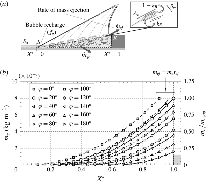
). As indicated in the schematic in figure 16(a), for swept interactions, an additional component
 ${\dot{m}}_{\unicode[STIX]{x1D711}}$
is to factor in the spanwise mass flow rate effect, which intrinsically contributes to an effective local depletion as part of the separated flow is swept towards outer planes.
Estimated evolution of separated mass per unit span carried by large-scale shear-layer eddies
 $m_{\unicode[STIX]{x1D700}}$
(
 $=\int _{0}^{t_{c}}{\dot{m}}_{x}\,\text{d}t$
, based on (4.2)). Right axis indicates reference to eddy mass upon ejection within the
 $\unicode[STIX]{x1D711}=0^{\circ }{-}30^{\circ }$
range, with local
 $m_{_{\unicode[STIX]{x1D700}},ref}\approx 8\times 10^{-6}~\text{kg}~\text{m}^{-1}$
, and whereby the rate of mass ejection is
 ${\dot{m}}_{ej}=m_{\unicode[STIX]{x1D700}}\,f_{ej}$
(
 ${\dot{m}}_{ej,ref}\approx 0.07~\text{kg}~\text{s}^{-1}~\text{m}$
).

As further illustrated in figure 18, the local entrainment rate at the scale of large shear-layer eddies
 ${\dot{m}}_{x}$
(
 $=\text{d}m_{\unicode[STIX]{x1D700}}/\text{d}t$
) is thus expected to increase over the separation length and attains its highest values upon ejection. As such, the rate of mass depletion may be seen to effectively result from the continued entrainment as eddies convect along the bubble all the way down to their departure near the obstacle, i.e. the integral effect of the tendency in figure 18, as eddy growth is sustained (refer to Estruch-Samper & Chandola Reference Estruch-Samper and Chandola2018). For two-dimensional axisymmetric separation in the latter (
 ${\dot{m}}_{\unicode[STIX]{x1D711}}\approx 0$
), the entrainment-recharge dynamics were in turn found to lead to a characteristic time scale of bubble breathing
 $T_{o}=M_{B,rev}/{\dot{m}}_{ej}$
, where
 $M_{B,rev}=\unicode[STIX]{x1D705}_{R}0.5\unicode[STIX]{x1D70C}_{B}Lh$
is the local mass of the reverse flow within the bubble, corresponding to
 $\unicode[STIX]{x1D705}_{R}\approx 50\,\%~(=M_{B,rev}/M_{B})$
relative to local separated mass. This is in principle coherent with the present evaluation in figure 19, as discussed next.
Summary of swept STBLI results: azimuthal variation in characteristic frequency at separation
 $St_{o,\unicode[STIX]{x1D6FF}}$
and at ejection location
 $St_{ej,\unicode[STIX]{x1D6FF}}$
, together with the respective
 $f_{o}/f_{ej}$
ratio (
 ${\approx}St_{o,\unicode[STIX]{x1D6FF}}/St_{ej,\unicode[STIX]{x1D6FF}}$
) and local axial separation scale
 $L/\unicode[STIX]{x1D6FF}_{o}$
(
 ${\sim}l_{sh}/\unicode[STIX]{x1D6FF}_{o}$
, where
 $l_{sh}$
is shear-layer length). Dashed lines mark the swept STBLI region of interest as per figure 16(b), with results taking symmetry at
 $\unicode[STIX]{x1D711}=0^{\circ }$
. The grey shaded area indicates
 $h/\unicode[STIX]{x1D6FF}_{o}<1$
range (as per figures 13 and 16
a,b).

4.3 Swept bubble recharge and separation shock instability
Two key observations are drawn from the above: (i) the bubble’s breathing and ejection rates are immediately correlated within a given streamwise path, with the entrainment-recharge process locally driving the low-frequency instability of the separation shock, i.e. as a function of the properties at
 $X_{ej}^{\ast }$
; and (ii) as per the noted tendencies, the bubble’s recharge is bound to be primarily driven at separation, where the flow would first act to compensate for the mass depleted downstream upon ejection, at a given
 $\unicode[STIX]{x0394}\unicode[STIX]{x1D719}$
.
As per the views of the mechanism in Estruch-Samper & Chandola (Reference Estruch-Samper and Chandola2018), to later account for the sweep effect through local
 ${\dot{m}}_{\unicode[STIX]{x1D711}}$
contributions, the frequency of bubble recharge may be seen to scale locally as
 $$\begin{eqnarray}f_{o}=\frac{{\dot{m}}_{ej}}{M_{B,rev}}\approx \unicode[STIX]{x03C0}\unicode[STIX]{x1D6FC}_{\unicode[STIX]{x1D700}}\unicode[STIX]{x1D709}_{B}\frac{L}{h}\unicode[STIX]{x1D6FF}^{\prime 2}X_{ej}^{\ast 2}\,f_{ej}\approx C_{\unicode[STIX]{x1D700}}\,f_{ej},\end{eqnarray}$$
where variations in separation aspect ratio
 $L/h$
and shear-layer spreading rate
 $\unicode[STIX]{x1D6FF}^{\prime }$
, noting
 $\unicode[STIX]{x1D6FF}_{\unicode[STIX]{x1D714},ej}=\unicode[STIX]{x1D6FF}^{\prime }(LX_{ej}^{\ast })$
, may be deemed negligible for this assessment, thereby approximating to a constant
 $C_{\unicode[STIX]{x1D700}}$
for evaluation purposes, hence
 $f_{o}\approx C_{\unicode[STIX]{x1D700}}\,f_{ej}$
.
The above is consistent with the present evaluation in figure 19, where the low-frequency instability of the bubble is seen to remain at a constant level of
 $f_{o}\approx 0.08f_{ej}$
within
 $\unicode[STIX]{x1D711}=0^{\circ }$
–
 $120^{\circ }$
(
 $\unicode[STIX]{x1D6EC}\leqslant 30^{\circ }$
), as the extent of separation is gradually reduced (i.e. complying with a constant
 $C_{\unicode[STIX]{x1D700}}\approx 0.08$
). The above is noted to correspond to practically twice as high a value than the
 $C_{\unicode[STIX]{x1D700}}\approx 0.04$
in the reference axisymmetric case (
 $L/\unicode[STIX]{x1D6FF}_{o}=30$
), which was as well observed across the range of axisymmetric interactions at
 $M_{e}\geqslant 3$
– for supersonic convection Mach numbers, and whereby
 $L/\unicode[STIX]{x1D6FF}_{o}\geqslant 5$
(
 $h/\unicode[STIX]{x1D6FF}_{o}\geqslant 1$
) – in the preceding phase of the programme. The relatively higher
 $f_{o}/f_{ej}$
ratio for the present swept STBLI is thus in principle consistent with the presence of a spanwise
 ${\dot{m}}_{\unicode[STIX]{x1D711}}$
contribution, which is bound to act as an additional source of local mass depletion within a streamwise plane, as part of the separated flow is laterally swept – noting that it could be strictly factored in within the above but this is here limited to simple evaluation of the unfolding tendencies (given the related inaccuracies in determining the latter contribution).
4.4 Final remarks
Overall, the scope of the investigation has lain in documenting the time-resolved wall pressure over a swept STBLI with large-scale separation
 $L/\unicode[STIX]{x1D6FF}_{o}=26$
, priming high measurement resolution and spectral range (reliably up to
 ${\sim}50$
kHz, over durations of order
 $(10^{3}{-}10^{4})T_{o}$
), with the reference flow being an axisymmetric turbulent boundary layer and hence enabling us to discard added effects to some extent present in planar configurations. Results confirm that relatively higher pulsation frequencies are broadly to be expected in swept turbulent interactions, largely due to the lateral convection inherent to the sweep effect towards farther azimuthal planes, which – from the perspective of the entrainment-recharge mechanism – essentially acts to enhance the effective ‘mass depletion’, locally prompting a more frequent recharge of the bubble. It is further shown that the bubble breathing mechanism does not adopt a global pulsation frequency, but instead changes locally along the swept separation line – in turn influencing the separation shock instability, which is found to vary proportionally to
 $f_{ej}$
in the spanwise direction, and thus unveiling the localised nature of the breathing dynamics which drive the large-scale pulsations of the bubble.
While the effective spanwise flow rates and relative mass entrainment variations are highly challenging to determine, both experimentally and numerically (in part given the high frequencies and large gradients within high-speed turbulent separation), it would be of particular interest to elucidate how the varying entrainment dynamics of the swept shear layer are modified, so as to evaluate how the bubble breathing mechanism responds locally in a wider range of swept separation conditions and configurations. Indeed, further comparisons would eventually allow to clarify the potential coexistence and relative contribution of other influences, and to do so, special care should be placed towards ascertaining that the unsteady shear layer and shock pulsations are resolved at sufficiently high space/time resolution, ideally over long durations for reliable interpretation.
5 Conclusions
The unsteadiness of a large-scale swept STBLI, induced by a canonical surface discontinuity over a turbulent axisymmetric base flow (
 $90^{\circ }$
step, with spanwise-varying height) has been experimentally investigated at Mach 3.9 and high Reynolds number. The perturbations radiated by large shear-layer eddies emerge close downstream of separation and bear a dominant influence at high to mid frequencies as they evolve over the recirculation zone, at supersonic convection velocity. Eddy growth is intrinsically sustained through entrainment – in part from the separated flow – up to their departure, draining the bubble at varying rates over its span. The process of mass depletion is effectively driven by the continued mass entrainment as eddies convect along the bubble all the way down to their ejection and is in great part dictated by the local scale of separation (i.e. the shear layer’s path up to ejection), as well as by shear later spreading rate and related variables (convection Mach number, entrainment dynamics, etc.). This is maintained within the moderately swept region (
 $\unicode[STIX]{x1D6EC}\leqslant 30^{\circ }$
), whereby a well-developed recirculation is formed.
While not strictly exclusive of other influences – e.g. incoming turbulence, Görtler-type effects, a potential selective-amplifier behaviour of the separation, etc. – results overall sustain the view of the separated shear layer as a prevalent contributor to STBLI unsteadiness. Variations in the mass entrainment capabilities of the swept eddy structures remain particularly challenging to estimate, yet the observed acceleration of shock pulsations at locations farther from the reference plane, where higher values of low-frequency unsteadiness are found, are strongly consistent with the views of the entrainment-recharge mechanism as the primary driver of low-frequency unsteadiness. Results suggest that the relatively higher pulsation rates for swept interactions are largely due to an enhancement of the effective mass depleted locally within the bubble. In particular, the separation shock’s instability is found to adjust locally in response to the downstream rate of ejection, with the instability at separation (associated with bubble recharge) here noted to adopt relatively higher breathing frequencies, exceeding twice the respective rates in analogous axisymmetric separation.
Overall, the low-frequency instability at separation complies with a frequency of bubble breathing
 $f_{o}$
as the ratio of ‘local mass depletion rate’ to ‘reversed flow mass’, extending this view to swept STBLIs with well-developed separation. Results evidence the highly localised nature of the mechanism, largely imposed by the swept shear-layer properties upon ejection. Similar low-frequency levels are noted near reattachment, yet broadband given the added influences by this stage (e.g. centrifugal instabilities), suggesting that recharge is primarily modulated via separation as near-wall incoming flow is naturally allowed in for its replenishment.
Acknowledgements
This research was supported by the Ministry of Education (MOE) Singapore through AcRF Tier 1 grant R-265-000-527-112. X.H. is a recipient of National University of Singapore (NUS) PhD Scholarship.