Today, developed countries universally fund public primary education. However, this was not always true. In England, the United States, Prussia, France, and other countries, many children were educated in a thriving private sector before the establishment of fully tax-supported public primary schools.Footnote 1 Even in areas of the United States where schools received public support, parents often paid substantial tuition charges, known as rate bills.Footnote 2 In the average state in 1850, these private contributions accounted for about 20 percent of public school funds.Footnote 3
During this period, high fractions of children attended primary school and were literate.Footnote 4 For example, Albert Fishlow states that the common school movement was most active in areas where enrollment rates were already high, and that “the reform movement attained its greatest immediate success in the triumph of New England public schools over the flourishing private alternatives” rather than in raising educational levels.Footnote 5 E. G. West argues “we lack firm evidence to show education was not already universal prior to the establishment of laws to provide a schooling that was both compulsory and free.”Footnote 6 Claudia Goldin and Lawrence Katz summarize historians' work on New York and Massachusetts and conclude that enrollment rates were similar even though the timing of the free school laws that outlawed private rate bills differed by 41 years.Footnote 7 That being the case, why did voters choose to fully fund primary education?
The mid-nineteenth-century United States is a good place to test explanations of voter support for public education for several reasons. First, during this period states erected the institutions that allowed for the expansion of public education, including laws permitting or requiring local property taxation, restricting public funds to government run schools, and banning private fees at public primary schools.Footnote 8 Second, there was significant regional variation during this period. Rural New England areas established “common” primary schools by the early 1800s that were open to all children, and these expanded across other northern states. Northern states also tended to have relatively low rate bill charges. In contrast, large fractions of Southern students were educated in private schools until after the Civil War, and Southern public schools relied heavily on private contributions. The third reason why this period is a natural test case for political economy models is that voters were the agents who enacted most of the changes. During the nineteenth century, voters chose direct local taxation and full public support directly in referenda or indirectly through state legislation or new constitutions.
This article brings together two strands of literature to address this question. First, a body of theoretical literature models potential voter motivations for publicly funded education. A second body of empirical work by Goldin and Katz connects the rise in secondary school attendance to wealth and demographics, although it does not explicitly examine public funding.Footnote 9
This article makes two contributions to these literatures. First, the empirical work examines differences in public subsidies across states in 1850 and 1860 to test two political economy models. In median voter style “pure redistribution” models, public education is a way decisive voters transfer wealth (in the form of education subsidies) to themselves. In “external benefits” models, however, decisive voters transfer wealth to others to realize the gains that come from higher general levels of education. The theoretical section of the article shows that the relationship between the distribution of wealth and public subsidies can help to distinguish these two motivations. “Pure redistribution” models imply that when mean income is farther above the decisive voter's income, ceteris paribus, this lower tax price will lead to higher public subsidies. Inequality in this sense raises transfers. “External benefits” models show that there are some conditions under which greater equality might be associated instead with higher transfers: when the decisive voter has wealth above the mean, but experiences large external benefits, societies with a large group of the moderately wealthy will have larger public subsidies.
Implicit in the “external benefits” model is the assumption that public funding of education raises education levels. This article makes a second contribution by directly examining whether the public share of education funding increased educational attainment, a fact that has been questioned by some economists and historians.Footnote 10 Most of this research uses case studies of northeastern states and examines how a free school law affects attendance. This article instead examines how the public-private mix of funds affects attendance, looking across all states. Using the mix of funds instead of a law change is useful in this period because private contributions were often already declining to negligible levels just before passage of a free school law. As a result, the funding mix varied widely among states with similar laws. In addition, the empirical approach explicitly accounts for the fact that attendance rates and public provision may be determined simultaneously. To identify the causal effect of public funding on attendance, the analysis uses variations in federal land grants and federal deposit funds as instruments for public funding. These federal grants were determined by the date of statehood and the number of political representatives and were not conditioned on attendance rates or other features of the education system.
VOTER MOTIVATIONS FOR PUBLIC FUNDING OF EDUCATION
Voting for Public Education: Redistributive Model
One class of theoretical models argues that public education is essentially a mechanism decisive voters use to transfer resources from others to themselves. Dennis Epple and Richard Romano derive several results that hold when a publicly provided good can be purchased in the private sector or augmented with substantial private contributions. This was clearly the state of primary education in the 1800s.Footnote 11
To illustrate the relevant results of this model in a simple case, suppose utility depends on education services, ei, and private consumption, ci. Education services are the sum of government purchases that everyone consumes, g, and individual private supplements, si: ei = g + si.Footnote 12 This “supplementing” is consistent with the practice in many areas of tax-supported teacher salaries for a certain number of months, with additional months of education purchased privately. However, some private contributions were also required for attendance, as with rate bills; this case will be discussed below.
If g is provided by a proportional tax on wealth, the government budget constraint is g = t* m, where m is mean wealth. Individual pretax wealth is defined as yi.Footnote 13 Normalizing ci and ei so that the units are in dollars, the individual's budget constraint is ci + ei = yi(1–t) + g or

When si is positive, additional education is purchased in the private sector. The private first order condition in this case is

On the other hand, when si is zero and the marginal dollar spent on education comes from the public sector, the first order condition is

In other words, all individuals face a uniform price of education in the private market. Each individual's price of additional government spending on education, however, varies in relation to the individual's tax price, which is the ratio of own wealth to mean wealth.Footnote 14
An individual's support for public funding therefore depends on an income effect and a substitution effect. If education is a normal good, an increase in a voter's wealth increases demand for education, whether provided privately or publically. However, higher wealth also decreases demand for public funding via the effect on the tax price. An individual with wealth above the mean faces a tax price that is higher than the private price of education: yi/ m.>1. This means that one, all individuals with wealth above the mean oppose public education, preferring to purchase education privately, and two, holding constant the wealth of the decisive voter, a lower tax price (high mean wealth relative to own wealth) implies more redistribution.Footnote 15
Voting for Public Education: When There are External Benefits
A second class of models argues that voters may receive some benefit from the education of others, either because of altruism or because higher education levels lead to efficiency gains. Several papers suggest that public education may be associated with social gains, whether due to faster growth, lower crime, a better functioning democracy, socialization of immigrants, greater homogeneity, network externalities, resolution of credit constraints, or higher returns to physical capital.Footnote 16 As a result, individuals vote to subsidize others' education when the benefits of public funding (both the subsidy to themselves and the external benefits from others' education) exceed their taxes.
The model above can be modified to show this.Footnote 17 Individual utility now depends on own consumption, own education, and the benefits that come from education of others, b. For simplicity, assume that these external benefits do not depend on an individual's wealth: Ui = U(ei, b, ci).
In this case, when the marginal dollar spent on education comes from the public sector, the first order condition is

In contrast to the previous model, this now means that some individuals with wealth above the mean will support public education because the external benefits are large enough to outweigh their positive net taxes. These “moderately wealthy” individuals lie in the interval where Ub/Uc ≥(yi/ m)–1. Very wealthy individuals at even higher points in the wealth distribution still oppose public subsidies, not because they do not benefit from the externalities, but because their tax burden is higher than the expected benefits. The more compressed the wealth distribution is around the mean, the more individuals will fall into the “moderately wealthy” category where Ub/Uc ≥(yi/ m)–1 and the external benefits are enough to offset the difference between the public tax price and the private cost of education.
If the decisive voter is someone with wealth below the mean, political support by the “moderately wealthy” is not important. However, in this time period wealth and political influence were related. Although most states did away with property-based voting restrictions for national elections by 1850, several had poll taxes, literacy and residency tests for immigrants, prohibitions on pauper voting, and property requirements for local elections.Footnote 18 In this case, the decisive voter may well have been an individual with wealth above the mean.
Funding Education with Mandatory Private Contributions
The above models assume that private supplements are voluntary. Raquel Fernandez and Richard Rogerson discuss the case where private contributions are instead mandatory (e.g., tuition charges), which was true of rate bills.Footnote 19 If households are credit constrained, required private contributions may restrict access to the public subsidy: poor children who cannot afford the tuition charges do not attend school. In this case, tax prices now depend on own wealth, mean wealth, and the fraction of children attending school. This fraction in turn depends on the wealth of the poor relative to the cost of education. The voting equilibrium in this case is more complex and depends on the sizes of coalitions of families, as shown in Fernandez and Rogerson. Voters are not only concerned with the level of government expenditures, but also with the degree to which total expenditures are subsidized, as this affects the group who attends school.
There are several implications of this extension. First, increased subsidies lead to higher attendance rates for the poor when credit constraints are binding, but attendance rates for wealthy families are less responsive to changes in public share of education funding.
Second, partial subsidies of education may be an equilibrium outcome. Holding the cost of education constant (e.g., the cost to become literate, or the cost of nine months of primary schooling), increasing the public subsidy defrays required parental contributions and acts as a cash transfer for families already purchasing education. However, greater subsidies also mean that more of the poor will attend, dividing the tax revenue by a larger number of students. These two competing forces can lead to partial subsidies. The empirical work below accordingly focuses on the fraction of all education spending that comes from public sources as the measure of the government subsidy, rather than the level of government spending.
Third, in this model it is still the case that higher inequality leads to greater subsidies when there are no external benefits. This is for two reasons. The decisive voter still faces a tax price related to own wealth relative to mean wealth, and as before, a greater gap between mean and decisive wealth leads to higher transfers. In addition, if the wealth of the poor is much lower than the cost of education, subsidies can be large and the private cost will still exclude many students, further lowering the tax price to the families that consume education. Again, external benefits are necessary to lead to a predicted negative relationship between inequality and subsidies.
EMPIRICAL STRATEGY
The empirical analysis distinguishes the models in two ways. First, the models contain opposite predictions about the effects of wealth dispersion on public funds. In the purely redistributive model, a lower tax price—more dispersion between mean and decisive wealth—implies more redistribution. In the external benefits model, a larger fraction of the moderately wealthy—greater compression just above the mean—implies more redistribution. Both models are concerned with the dispersion at the center of the distribution as opposed to greater inequality arising from changes in the extreme tails of the distribution.Footnote 20
The empirical analysis uses the difference between mean and median wealth as the measure of central dispersion. This is related to the tax price, being exactly the tax price if the median wealth individual is decisive. It is also related to the central dispersion of wealth: in the lognormal distribution, the ratio of the mean to the median is related to standard deviation and therefore to the fraction of individuals with wealth just above the mean.Footnote 21
The median wealth individual is not necessarily the decisive voter, but it is not clear if the decisive voter would have wealth above or below the median. Epple and Romano and Jon Sonstelie show that private alternatives or supplements to public education can reduce the position of the decisive voter in the distribution relative to the median.Footnote 22 On the other hand, Roland Benabou argues that if wealthier voters have more political influence than poorer voters, this will raise the position of the decisive voter in the distribution.Footnote 23 Additional specifications replicate the analysis using the gap between mean wealth and wealth at the 25th or 75th percentiles. These results are similar; they are not presented but are available on request.
The second test to distinguish the two models concerns the effect of public funding on attendance rates. For the external benefits model to hold, it must be the case that a greater share of public funding raises education levels. Otherwise, there would be no reason for wealthy voters to support public funding. However, in the pure redistribution model public subsidies may either raise education levels or leave them unchanged. When private contributions, si, for an individual are positive, increases in g are like cash transfers, reducing si and leaving education (ei) unchanged. If greater public support leads to no change in educational outcomes, as reported by some historians, this could only be consistent with the purely redistributive model; a finding that education levels rise with g could be consistent with either model.
The baseline econometric specifications then are


where g measures public subsidies in state i and year t, d is the difference between mean wealth and median wealth (wmean – wmedian), w is median wealth, attend measures attendance rates, and X and Z are vectors of other demographic controls. These include the number of white school aged children per household, the proportion of the white population that are immigrants, the fraction of churches that are Catholic, and the fraction of the population that is urban (living in places with 2,500 or more inhabitants). I restrict attention to white households because of racial restrictions in voting.Footnote 24 Goldin and Katz suggest that an “overlapping generations” model of education may apply, and the regressions accordingly also include the fraction of the white population over 65 years of age.Footnote 25 Finally, the regressions include a dummy for the western states that did not achieve statehood until after 1850. These states are also notable for being settled much later and for being much less densely populated.
Equation 5 is estimated at the state level to accommodate the fragility of the data sources. Manuscript data at the county level in 1850 show counties with missing funding, missing students, or improbable relationships between the levels of students and funds. The aggregated state data appear to be more internally consistent and are also consistent with the historical descriptions of funding systems in various states, implying that the errors at the local level do not appear to be systematic. The public funding regressions therefore focus on state-level variables, where measurement error may be less problematic. While many school funding decisions were made at the local level, there is still substantial variation across states due to legal and other institutional state differences. Attendance regressions are presented for individual children, but include the state-level variables.
However, using state averages is problematic if substantial variation exists across local areas and the state measures are not simply aggregated local measures. For example, Louisiana has the highest gap between mean and median wealth at the state level. If this is because wealth is unequally distributed within counties across the state, this state average is reflective of local conditions. However, if some localities are (uniformly) high wealth and others are (uniformly) low wealth, the state difference between mean and median wealth is a poor proxy for the relevant local variables.Footnote 26 For the subset of variables that are available at the county level, I average the county measures and examine the correlation between the average county measure and the state-level measure. For the fraction of immigrants, proportion who are older than 65 years of age, median wealth, and the difference between mean and median wealth, the correlation between the state average and the average county is high (above .8). The one exception is proportion of churches that are Catholic—there the correlation is .2, because Catholic churches are highly concentrated in a few counties. I view these generally high correlations as indicating that the state-level analysis likely approximates the aggregated local decisions. However, to the degree that there is still some measurement error, the coefficients may be understated.
Identifying the Effect of Public Subsidies
The estimation is complicated by the fact that attendance and public provision are likely jointly determined.Footnote 27 If high opportunity costs of time mean that a child would not attend regardless of the funding scheme, the parents are unlikely to support public education. This means that b2 may not reflect the causal effect of subsidies.
To correct for this problem, I use an instrument variables approach. This IV approach has two stages: in the first stage, I predict the public share of education funding using all independent variables as well as other variables that affect public funding but are not themselves related to attendance. The second stage uses the predicted values in the attendance regressions. I use two federal grants for public education as instruments for g.Footnote 28 The federal government issued National Land Grants for public schools to new states beginning with Ohio in 1802. Between 1802 and 1850, each state admitted was allotted one-sixteenth section of its lands; after 1850 two-sixteenth sections of land were allotted. I use allotted acres per white school-aged child as the first instrument for public provision. This varies with the status and date of statehood, the land area, and the school-aged population. The federal government made a second intervention in 1837, when it disbursed “Deposit Fund” monies from the sale of federal public lands to form endowments for public schools. States varied in the number of quotas they received according to the number of representatives each had. The amount of surplus fund per white school-aged child is the second instrument. Key to my strategy is that both instruments affect the level of public funds available for education, but neither was predicated on student attendance rates in public schools.Footnote 29 However, there is likely measurement error in this variable. Ellwood Cubberley and Edward Elliott report that many states borrowed against the deposit funds for noneducation purposes.Footnote 30 By 1850 five states (Arkansas, Georgia, Mississippi, New Jersey, and Pennsylvania) had depleted their funds. Seven other states had depleted theirs by the end of the Civil War. As a result, there is likely to be measurement error in this variable, attenuating the results.
Note that it is also not clear how these earmarked federal funds will affect the public share of funding because funds are fungible: states could respond to the federal funds by reducing their state contributions to education. Economists who have examined a similar type of earmarking in a contemporary setting have found mixed results: Neva Novarro and William Evans and Ping Zhang find that earmarking lottery funds for education does not increase education spending by the full dollar amount of the earmark, but that it does increase education spending by more than non-earmarked funds.Footnote 31 Samuel Cooper and Elchanan Cohen discuss other studies with more mixed results.Footnote 32
DATA
Data come from the Decennial Census reports of 1850 and 1860, based on two of the surveys. The Survey of Social Statistics surveyed states and minor civil divisions about schools, assessed wealth, and churches (among other things). Data from Household Survey come from the IPUMS 1-percent samples. These individual returns contain demographic information including school attendance, age, nativity, race, and the value of real property in 1850 and 1860 and personal property (if above $100) in 1860. Means of these data are reported in Table 1, with specific sources for each variable included in the Appendix.
MEANS AND STANDARD ERRORS OF VARIABLES IN STATE REGRESSIONS
(Means are only for states with all data in sample.)

Notes:
*For 1840 this is the sum of “Academy and grammar school students” and “Primary and common school students” divided by number of white children ages 5–14 years old. For 1850 this is the white attendance rate for children ages 6–15 calculated from the Census IPUMS 1-Percent Samples of Individuals. The rate is for children who report attending school at any time during the year.
Sources:
See the Appendix for construction of variables and sources.
Table 1 presents data for 1850 and 1860. Some schooling data is also available for the years after the Civil War and for 1840. However, the 1840 surveys do not provide funding information for schools or school attendance for individuals. Post-Civil War data is also not used. It may not reflect voting equilibria for all states if schools were destroyed during the Civil War. The compulsory schooling movement also began in the 1860s, complicating the interpretation of attendance regressions after 1860.Footnote 33 Later years also reported the education data in forms that are not exactly congruent with the 1850–1860 censuses. In general, parallel regressions for 1870 do not yield consistent results and are sensitive to the treatment of Southern states.
Measuring Wealth
The censuses of 1850 and 1860 contain wealth information from two sources: the individual returns and total assessed values reported in the Compendia of the Censuses. Because the assessed values were used for tax purposes, they are probably most related to the relevant tax price. However, they can only be used to compute the average. As the measure of d, the regressions use the difference between mean assessed household real property and the median of household real property as reported by individuals.Footnote 34
Measuring Public Subsidies
Estimating equations 5 and 6 requires a measure of g, the level of public subsidies. The Survey of Social Statistics reports school revenues at “Public Schools” and “Academies and other schools” from “taxation,” “other public sources,” “endowments,” and “all other sources” (i.e., tuition or rate bills). I measure g as the fraction of revenues at all schools in a state (both public and private) from “taxation” and “other public sources.”
This measure is most appropriate for several reasons. First, including all schools accommodates the blurred distinction between public and private schools in this period.Footnote 35 Second, the fraction of funds from public sources also reflects the degree to which private contributions were used and may have excluded some children from attending.Footnote 36 This is in contrast to a measure like public expenditures per pupil, which will not measure the degree to which individuals might be restricted from attendance by required contributions. It also abstracts from different prices of education across states, which may have led to higher or lower expenditures.
Third, this continuous measure captures variation in public subsidies, even when state laws might be similar. Sometimes laws lagged changes in behavior: Goldin and Katz state that (at least in the North) rate bills gradually declined, and the date of passage of a “free school law” does not necessarily identify when private contributions became an insignificant source of funds.Footnote 37 In other areas, behavioral changes lagged the laws. Carl Kaestle reports that in Ohio, Illinois, and Michigan, early local taxation laws were ineffective or were repealed and later reinstated before finally taking hold.Footnote 38 Finally, “public school laws” did not necessarily bind on all districts simultaneously.Footnote 39 This makes it difficult to use the timing of state law changes as a way to determine the effect of public subsidies on education levels.
However, in some areas “academies” mostly referred to private secondary schools, while in other areas they included many private primary schools. The fraction of school funds from public sources may therefore conflate public subsidies with the amount of secondary schooling. To deal with this problem, the regressions control for the fraction of children attending school that are younger than 15 years of age. These younger children are presumably attending primary schools. This fraction is calculated using the individual school attendance reports in the IPUMS 1-percent sample of census records.
Trends in Public Funding and Attendance
To provide a sense of the overall trends and regional differences in public funding and attendance in this period, Figures 1, 2, and 3 plot the trend in the fraction of educational revenues that came from taxation and public sources and the trend in attendance for years 1840–1880. Dotted lines are used when the variables are not identically defined across census years. The figures group states into six regions with roughly comparable historical experiences: New England, the Mid-Atlantic, the Midwest (states that achieved statehood prior to 1850), the West (states that achieved statehood after 1850), Confederate states, and Border states (slave states that did not officially join the Confederacy).Footnote 40
PROPORTION OF TOTAL EDUCATION REVENUES FROM PUBLIC SOURCES BY REGION, 1850–1870

Figure 1 shows both the rise in public provision across the states during the mid-nineteenth century and the considerable regional variation. In 1850 about 40 percent of educational revenue came from taxation and other public sources. This rose to nearly 70 percent by 1870.Footnote 41 New England, Midwestern, and to a lesser extent Mid-Atlantic states all began with relatively high levels of public subsidies. The West and Border states lagged, but by 1870 they had levels comparable to the other regions. Public subsidies for education in the South increased at a slower pace. Only about a third of total educational funds came from public sources in the South in 1850, and the majority of educational revenues in Confederate states were still from private sources by 1870. These means obscure differences among states within a region. For example, in New Jersey, 68 percent of educational revenues came from private sources in 1850, while 28 percent did in Pennsylvania. Similarly, in South Carolina private contributions were 90 percent of public school revenues in 1850, but were 40 percent of public school revenues in North Carolina.
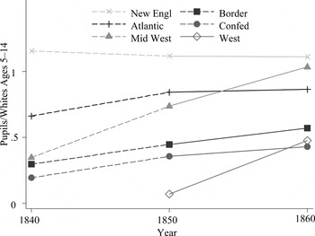
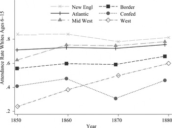
Attendance rates are reported in Figures 2 and 3—the two figures are from different surveys and cover different time spans. Figure 2 shows the trend in the ratio of pupils (in both “Academy and grammar schools” and “Primary and common schools”) to white children ages 5–14 from 1840 to 1860, as reported in the Survey of Social Statistics. Figure 3 shows the fraction of white children ages 6–15 who report attending school at any time during the year in the individual returns of the Household Census for 1850 through 1880. Together, these figures show that New England and the Mid-Atlantic states had high initial enrollment rates in 1840, with essentially stable enrollment rates after 1850. This is consistent with the observations of the historians who argue that public subsidies did not change enrollment. However, other areas show increases in enrollment over the period. Less settled areas (the Midwest in 1840 and the West in 1850) had initially low rates of school enrollment. These rates rose sharply in succeeding decades. Southern states also started out with low rates of school enrollment compared to Northern states. These rates rose before the Civil war. In most areas, attendance rates dipped in 1870. Although attendance rates recovered to a higher point by 1880, they still remained lower in the South than in any other region in the county.
WHITE ENROLLMENT RATES BY REGION, 1840–1860

RESULTS
Explaining Public Provision
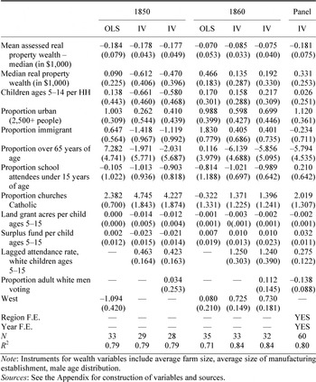
Table 2 reports the estimates of equation 5. The first three columns contain the results for 1850, and the next three are for 1860. For each year, a baseline set of OLS results is reported first, in columns 1 and 4, with the IV results in the succeeding two columns. The results show that the gap between mean and median wealth has a negative effect on the public share of education funding. The coefficient is always negative, generally significant, and is of an economically relevant magnitude. Moving from one standard deviation below the mean to one standard deviation above the mean in the wealth gap measure is associated with a 13 to 23 percentage point reduction in the fraction of education funds from public sources. Other demographic variables appear to play a more limited role.
ATTENDANCE RATES FOR WHITE CHILDREN AGES 6–15, 1850–1880

Federal land grants are generally significant, although the signs are negative in 1850. This may be due to correlation with the date of statehood, or it may be that states with larger land grants were more heavily reliant on the federal endowment and took longer to establish a system of direct taxation. The two federal variables are jointly significant in all of the regressions, suggesting that they are not weak instruments to predict subsidies in the attendance regressions.
A potential econometric issue with estimating the effect of the wealth gap on public subsidies is that greater public subsidies might lead to a more equal distribution of wealth.Footnote 42 However, Eric Hanushek and Julie Somers note that changes in education resources in the United States are
PROPORTION TOTAL EDUCATION REVENUES FROM PUBLIC SOURCES
(Huber-White robust standard errors are in parentheses.)

Note:
Instruments for wealth variables include average farm size, average size of manufacturing establishment, male age distribution.
Sources:
See the Appendix for construction of variables and sources.
not empirically associated with changes in the income distribution, implying that the potential endogeneity bias may not be severe.Footnote 43
To be cautious, the estimates in other columns of the table have two changes to deal with this potential bias. First, these specifications include measures of the extent of education ten years before. If the education system is persistent and affects the distribution of wealth, including this lagged measure would account for the observed correlation. The exact measure used is the fraction of white children ages 5–14 attending school ten years before (the attendance rate in 1840 in the 1850 regressions and 1850 in the 1860 regressions). Although it would be better to have an even longer lag, no systematic educational data exists prior to 1840.
Lagged attendance will control for the persistence of the education system and its effects on the distribution of wealth. However, to be cautious, the second specification also uses several instrumental variables to identify variation in the level and distribution of wealth that is independent of the educational system. Wealth holdings are partly determined by economies of scale in agriculture and manufacturing. Stanley Engerman and Kenneth Sokoloff note that the soil and climate determined the types of crops grown, which in turn affected economies of scale and therefore the distribution of land and wealth holdings.Footnote 44 Similar arguments would also hold in manufacturing where the type of product would determine optimal plant size. Average farm size and the average size of manufacturing establishments therefore act as instruments for the wealth variables. Both are likely to be unrelated to the mix of public and private funds.
I also use the age structure of the adult male population as a second instrument. This included the fraction of adult men ages 20 to 29, 30 to 39, 40 to 49, 50 to 59, and 60 and older. The point in the life cycle is related to wealth holdings. Given that the regressions already control for the fraction of the population over 65 years of age and children per household, the remaining variation in adult males' ages will likely be independent of the educational system of the state. Because the model is overidentified, I compute Hansen-J statistics to test the null hypothesis that the overidentifying restrictions are valid (implying exogeneity of the instruments).Footnote 45 The p-value associated with these tests range from .14 to .58, indicating failure to reject the null that the exclusion restrictions are valid. This implies that the model is appropriately estimated.
The second and fifth columns report estimates from these specifications. The lagged measure of public provision is highly significant and large, indicating sizable persistence in public funding. However, even conditional on the former education system, the coefficient on the mean-median gap is very similar in these estimates to the OLS estimates.
One final concern with these estimates is that there may still be substantial heterogeneity across regions that is correlated with the distribution of wealth. In particular, political systems in different areas might both affect the distribution of wealth and public funding. It is difficult to control for regional effects in the cross sections, as there are so few observations. However, the third and sixth columns reproduce the previous estimates using the fraction of adult white men in the presidential elections of 1848 and 1860.Footnote 46
The limited number of states requires a parsimonious specification. However, to be sure that the specifications include all relevant variables, I have conducted robustness checks with alternative variables. These include alternative measures of urbanization (population density and the fraction employed in manufacturing or agriculture), and various other measures of racial, linguistic, ethnic, or religious heterogeneity. None of these qualitatively change the basic results; all are available on request.
The final column addresses the issue of unobserved heterogeneity by reproducing the results using the entire panel and including year and region fixed effects. This controls for any overall national trend towards greater public subsidies or any unobservable characteristics that are constant within specific regions. Again, the panel results are similar to the other results: states with larger differences between mean and median wealth had higher public subsidies, even controlling for constant regional differences. Any time-variant regional differences are, of course, not accounted for in this fixed effect specification.
Effects of Public Subsidies on Individual Attendance
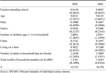
The findings thus far are consistent with “external benefits” motivating voters. However, if education levels did not increase in response to public subsidies, this makes an “external benefits” explanation less plausible. In this period, attendance is likely the most important measure of the education level. Table 4 therefore presents estimates of equation 6 and shows the effect of public subsidies on white children's attendance. (Table 3 reports the mean characteristics of the children in these regressions.) As noted, attendance and public funds are likely to be determined simultaneously, and federal land grants and surplus funds act as instruments to identify the causal effects of public provision. Note that the results in Table 2, which include the federal land grant instruments, are the first stage results.
MEANS OF VARIABLES USED IN INDIVIDUAL ATTENDANCE REGRESSIONS: WHITE CHILDREN AGES 6–14
(standard errors in parentheses)

Source:
IPUMS 1-Percent Samples of individual census returns.
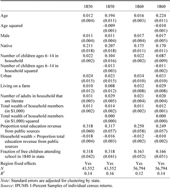
These regressions for individual children ages 6 to 14 in 1850 and 1860, with the attendance variable from individual family reports of whether or not a child attended any school within the last year. The regressions are based on a linear probability model.Footnote 47 The first and third columns report a linear model, with the second and fourth columns including quadratic terms in age, number of school aged children in the household, and wealth.
Table 4 shows that greater public subsidies in the state also increase attendance. A 25 percentage point increase in the fraction of total education funds from public sources (one standard deviation in 1850) increased the probability of attendance by about 7 percentage points in both years.
Total household wealth is also positively correlated with attendance. A one-standard-deviation increase in wealth was associated with a 6 to 8 percentage point increase in the likelihood of attending school. In the external benefits model, some voters subsidize the education of individuals who otherwise would not attend. This suggests that
RESULTS FOR INDIVIDUAL ATTENDANCE: WHITE CHILDREN AGES 6–14
(standard errors in parentheses)

Note:
Standard errors are adjusted for clustering by state.
Source:
IPUMS 1-Percent Samples of individual census returns.
public subsidies should increase the attendance rates of the poor relative to the rich. The regression also includes an interaction term between the measure of public subsidies and household wealth. The coefficient is always negative, indicating that the effect of public subsidies was higher for the poor than for the rich. This suggests that while public subsidies may have replaced private contributions for wealthier families, for children from poor families public subsidies led to a change in behavior. However, the effect of public subsidies is large enough and the interaction effect is small enough that only children from very wealthy families have no predicted change in attendance when education is more
EFFECT OF WEALTH AND PUBLIC FUNDING ON SUBGROUPS OF WHITE CHILDREN AGES 6–14
(Each line in the table reports results from a separate regression.)

Note:
All regressions contain the same variables as in Table 4.
highly subsidized. For example, only families with wealth above $31,000, or those in the top 0.4 percentile of the wealth distribution, would have no predicted increase in attendance from a one-standard- deviation increase in public funding. Public subsidies of education appear to have led to increased attendance rates for a large class of children.
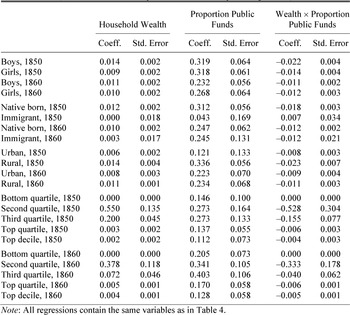
This raises the question of whether wealth and public subsides had the same effect on all groups of children. Table 5 reports results of regressions for separate subgroups of children (male/female, native/immigrant, urban/rural, and for separate quartiles of the wealth distribution). Each regression contains all of the variables reported in Table 4, but Table 5 only lists the coefficients for wealth, public funding and the interaction between wealth and public funds. Each row of the table represents a separate regression for the particular subgroup.
Two general patterns stand out. First, in 1850 the effects of public funds and wealth were more pronounced for some groups than others. The effect of wealth on native children was more than 10 times as large as the effect on immigrant children; the effect of public funds was nearly 6 times as great. Similarly, the attendance of rural children and children in the middle ranges of the wealth distribution were most affected by wealth and public funds. There was no difference for male and female children in the effect of public funds, and wealth had only a modestly larger effect on the attendance of boys.
The second pattern that stands out is how much less variation there is in the effect of public funds on various subgroups in 1860. By then, public funds had nearly identical effects on children of different genders, on natives and immigrants, and on rural and urban children. While public funds still had a larger effect on children from moderate wealth households, the differences by wealth group are much smaller in 1860 than in 1850. However, the effect of household wealth still displays a similar pattern to the 1850 results, with native born, rural, and moderate wealth children experiencing a larger boost in attendance rates than other children.
CONCLUSION
The mid-1800s was a period of considerable diversity in educational institutions across the United States: New England states generally had high levels of public subsidies at primary schools, Western states were settling and moving rapidly towards a system of public schools, while schools in the South were funded through significant private contributions until after the Civil War. Prior to public provision, there was a thriving system of private schools in urban areas, and parents in rural areas willingly paid for significant portions of their children's education. Why did voters choose to have schools that were free of parental contributions and provided through direct taxation?
This article argues that the relationship between the distribution of wealth and public provision can shed light on whether voters were choosing public subsidies as a wealth transfer to themselves or voting to subsidize others' education. In states with a smaller gap between mean and median wealth, education was more likely to be publicly funded than in other states that had similar median wealth but a larger wealth spread. Moving from one standard deviation below the mean to one standard deviation above the mean in the gap between mean and median wealth is associated with about a 15 percentage point increase in share of revenues from public sources. This is inconsistent with “purely redistributive” voter motivations, where the wealth gap is only related to the tax price. However, it is consistent with an “external benefits” story, where moderately wealthy voters realized benefits from the education of others, whether these benefits were due to efficiency, democracy, or personal altruism.
Furthermore, public funding had real effects on student attendance rates. A one standard deviation increase in the fraction of education revenues from public sources is associated with about an 8 percentage point rise in student attendance rates. The predicted increase is particularly large for children from poor families relative to those from wealthier families, and for native and rural children in 1850.
Data Appendix

Compendia of the Censuses:
1. Compendium of the Enumeration of the Inhabitants and Statistics of the United States as Obtained at the Department of State from the Returns of the Sixth Census by Counties and Towns, 1841.
2. The Seventh Census of the United States, 1850, Embracing a Statistical View of Each of the States and territories, arranged by counties and towns, 1850.
3. Statistics of the United States, (including mortality, property, &c.) in 1860; compiled from the original returns and being the final exhibit of the Eighth Census.
4. A Compendium of the Ninth Census (1872).