I. INTRODUCTION
Rubbers and rubber-like materials have been widely used in many industries because of their excellent properties, especially flexibility and durability. Considering the importance of rubber, however, the research outcome and its practical use on rubber have a long way to go. Hyperelastic rubber generally shows a nonlinear elastic behavior for large deformation. Viscoelasticity and hysteresis are also important characteristics of rubber. In addition, mechanical properties of rubber can easily change due to environmental effects such as heat, light, and aging. Therefore, it is hard to standardize property evaluation methods for rubber and even its constitutive equation and material properties. Kim et al.Reference Kim, Kim, Kim and Lee1 recommended using an equibiaxial tensile test method rather than a simple compression test method, which is sensitive to friction coefficient; however, because of the difficulty in making a rubber specimen and complicated testing process, the equibiaxial tensile test method has an impractical aspect. Lee et al.Reference Lee, Kim, Lee and Nahm2 therefore proposed a new method to evaluate material properties of hyperelastic rubber by using a nondestructive and in situ spherical indentation test. This method, however, considered only the oil-lubricated condition; thus, it has a drawback in practical use. In addition, the relatively shallow indentation depth causes inaccurate prediction of the third coefficient of the Yeoh model,Reference Yeoh3–Reference Yeoh and Fleming5C 3. Since C 3is related to the material behavior of rubber when the uniaxial engineering strain is over ∼1, this method detracts from the advantage of the Yeoh model.
This study examines indentation characteristics by using a more realistic coefficient of friction and a deeper indentation depth and suggests an improved indentation technique that can measure the static material properties of isotropic rubber. To achieve this, we analyze the effects of indentation depth and friction on indentation and choose a data acquisition point at subindenter to get the optimal characteristics of deformation. We reform then nondimensional functions, which map indentation load–displacement data into strain energy density and the first invariant (W–I 1) data by using triple-fitted polynomial functions for C 1, C 2, and C 3. To do this, C 1 is first obtained by the indentation load value corresponding to initial indentation depth, and by mapping using two nondimensional functions, C 2 and C 3are evaluated. We finally verify the effectiveness of the method to evaluate material properties of hyperelastic rubber materials.
II. CONSTITUTIVE MODEL
A. Comparison of the rubber models
The characteristics of rubber can be decomposed into time-independent and time-dependent behavior. Time-independent behavior considering finite deformation is described by isotropic hyperelastic models such as the neo-Hookean, the Mooney–Rivlin, the Ogden, the Yeoh, the Arruda–Boyce, and the Van der Waals model.Reference Yeoh4, Reference Mooney6–14 The models of rubber elasticity such as the statistical mechanics and phenomenological continuum mechanics theories have been developed by some different bases.Reference Treloar8, Reference Boyce and Arruda13 The statistical theory assumes randomly oriented long molecular chains of rubber to be idealized structures, whereas the phenomenological theory has been developed to conveniently describe the properties based on the continuum mechanics. As described by Treloar,Reference Treloar8 the phenomenological theories such as the Mooney–Rivlin, the Ogden, and the Yeoh models are based not on molecular concepts but on purely mathematical reasoning. In this study, we only deal with the phenomenological theory because it is convenient to describe the behavior of rubber materials in the continuum mechanics, and most studies including experimental works to evaluate the stress–strain properties of rubber use the phenomenological properties.
The invariant-based constitutive equations of rubber material are expressed by the relationship between strain energy density and strain invariants as follows:
 $$W\, = f(I_1 ,I_2 ,I_3 ),$$
where W is the strain energy density (or strain energy potential), which means the stored strain energy per unit volume, and I 1, I 2, and I 3 are the three invariants of the Green deformation tensor given in terms of the principal stretches (or extension ratios) λ1, λ2, and λ3as follows:
 $$I_1 \, = \,{\rm{\lambda }}_1^2 \, + \,{\rm{\lambda }}_2^2 \, + \,{\rm{\lambda }}_3^2 ,$$
 $$I_2 \, = \,{\rm{\lambda }}_1^2 {\rm{\lambda }}_2^2 \, + \,{\rm{\lambda }}_2^2 {\rm{\lambda }}_3^2 \, + \,{\rm{\lambda }}_3^2 {\rm{\lambda }}_1^2 ,$$
 $$I_3 \, = \,{\rm{\lambda }}_1^2 {\rm{\lambda }}_2^2 {\rm{\lambda }}_3^2 .$$
The strain energy density function in terms of the invariants is written as
 $$W = \mathop\sum\limits_{i + j + k = 0}^\infty {C_{ijk} (I_1 - 3)^i (I_2 - 3)^j (I_3 - 3)^k } .$$
Since rubber material is almost incompressible (I 3 = 1), Eq. (5) can be reduced to
 $$W = \mathop\sum\limits_{i + j = 0}^\infty {C_{ij} (I_1 - 3)^i (I_2 - 3)^{\,j} } .$$
Several reduced models of the polynomial form Eq. (6) have been suggested, such as the neo-Hookean model, the Mooney–Rivlin model, and the Yeoh model. The Mooney–Rivlin form is a linear function of the invariants I 1 and I 2, i.e.,
 $$W\, = \,C_{10} (I_1 - 3)\, + \,C_{01} (I_2 - 3).$$
The Mooney–Rivlin model is widely used because of its simplicity, but it is effective only in relatively small strain. For larger deformation, the Ogden modelReference Ogden11 is more appropriate than the Mooney–Rivlin form and can be expressed as
 $$W\, = \,\mathop\sum\limits_{i = 1}^n {{{{\rm{\mu }}_i } \over {{\rm{\alpha }}_i }}({\rm{\lambda }}_1^{{\rm{\alpha }}_i } + {\rm{\lambda }}_2^{{\rm{\alpha }}_i } + {\rm{\lambda }}_3^{{\rm{\alpha }}_i } - 3)} ,$$
where n, μ, and α are material parameters. It is noteworthy that the neo-Hookean and the Mooney–Rivlin models are special cases of the Ogden form.Reference Ali, Hosseini and Sahari15 The Ogden model, however, requires lots of fitting parameters, so that this method is effective only if sufficient experimental data are can be obtained. The Yeoh modelReference Yeoh3, Reference Yeoh4 and its extended modelReference Yeoh and Fleming5, Reference Beda16 have been thus suggested to be applicable for larger deformation with simple experimental data. The constitutive equation is represented by
 $$W\, = \,C_1 (I_1 - 3)\, + C_2 (I_1 - 3)^2 \, + \,C_3 (I_1 - 3)^3 .$$
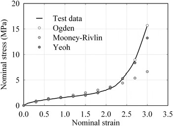
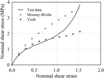
To compare the constitutive models, a uniaxial tensile test and a shear test have been performed for a vulcanized rubber. The Ogden, the Mooney–Rivlin, and the Yeoh coefficients are obtained from the fitting of the tensile test data. By using the coefficients, the nominal tensile stress–strain curves are generated and compared with the test data as shown in Fig. 1. Compared to the Mooney–Rivlin form, the Yeoh model is more suitable for describing the behavior of rubber materials. Moreover, although the Yeoh model is simpler than the Ogden model, it can follow well the experimental data including large deformation. Most of all, whereas the Mooney–Rivlin and the Ogden models often inaccurately predict the behavior for different modes by a single experiment, the Yeoh model can predict well the behavior in different deformation modes from data gained in just one deformation mode.Reference Ali, Hosseini and Sahari15 The shear stress–shear strain curves are then generated by the Yeoh and the Mooney–Rivlin coefficients, which are obtained from tensile test data, to compare them with experimental shear test data as shown in Fig. 2. The Mooney–Rivlin model shows large deviation from experimental data, but the Yeoh model can predict well the curve up to the shear strain is around 1.
Nominal stress–strain data predicted by the Ogden, the Mooney–Rivlin, and the Yeoh models of which coefficients are obtained from a uniaxial tensile test.

Nominal shear stress–shear strain data predicted by the Yeoh and the Mooney–Rivlin models of which coefficients are obtained from a uniaxial tensile test.

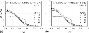
(a) W versus r/D and (b) I 1 versus r/D for various values of l/D where l is the distance from specimen surface to data acquisition depth before deformation and r is the projected distance from axisymmetric center after deformation.

As we assume incompressible materials, i.e., I 3 = 1, the strain energy density for an isotopic incompressible elastomer can be expressed as a function of I 1 and I 2 [W = f (I 1, I 2)]. In a strict sense, ∂W/∂I 2 has finite values.Reference McKenna and Zapas17, Reference McKenna and Zapas18 However, prior studies showed that ∂W/∂I 2 is sufficiently smaller than ∂W/∂I 1,Reference Yeoh and Fleming5, Reference Gregory19 and therefore, ∂W/∂I 2 is often assumed to be 0.Reference Yeoh and Fleming5, Reference Beda16, Reference Qi and Boyce20 If ∂W/∂I 2 is assumed to be 0, W can be represented as a function of only I 1. Coefficients for rubber materials can then be obtained from one single test, e.g., uniaxial tension test.Reference Ali, Hosseini and Sahari15 Therefore, a neo-Hookean model, a Yeoh model, and an Arruda–Boyce model are developed by neglecting I 2. We also use a strain energy density function based on I 1 [Eq. (9)]. In this study, the Yeoh model is thus selected as the constitutive equation.
B. The Yeoh model
The Yeoh model describes the behavior of rubber materials by W, I 1, and three coefficients C 1, C 2, and C 3. Hence, it is very important to investigate the effect of each coefficient on the stress–strain curve.
For a uniaxial tensile/compression test of incompressible rubber material, I 3 is equal to 1 ( ${\rm{\lambda }}_1^2 {\rm{\lambda }}_2^2 {\rm{\lambda }}_3^2 $ = 1). In addition, the principal stretches perpendicular to the tensile/compression direction are identical (λ2 = λ3), the following equations can be easily obtained:
 $${\rm{\lambda }}_2^2 = {\rm{\lambda }}_3^2 = 1/{\rm{\lambda }}_1 ,$$
 $$I_1 = {\rm{\lambda }}_1^2 + 2/{\rm{\lambda }}_1 ;\,\,\,{\rm{\lambda }}_1 \, = 1 + {\rm{\varepsilon }}_1 .$$
For uniaxial tensile/compression tests, the nominal stress, σ1, can be written as follows:
 $$W = \int {{\rm{\sigma }}_1 } \,d{\rm{\varepsilon }}_1 \, \leftrightarrow \,{\rm{\sigma }}_1 = {{\partial W} \over {\partial {\rm{\varepsilon }}_1 }} = {{\partial W} \over {\partial I_1 }}{{\partial I_1 } \over {\partial {\rm{\lambda }}_1 }}{{\partial {\rm{\lambda }}_1 } \over {\partial {\rm{\varepsilon }}_1 }}.$$
The first derivative of Eq. (9) with respect to I 1is
 $${{\partial W} \over {\partial I_1 }} = C_1 + 2C_2 (I_1 - 3) + 3C_3 (I_1 - 3)^2 .$$
Substituting this equation [Eq. 13] and Eqs. (11) and (12), we obtain
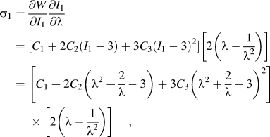 $${\rm{\sigma }}_1 = {{\partial W} \over {\partial I_1 }}{{\partial I_1 } \over {\partial {\rm{\lambda }}}} = [C_1 + 2C_2 (I_1 - 3) + 3C_3 (I_1 - 3)^2 ]\left[ {2\left( {{\rm{\lambda }} - {1 \over {{\rm{\lambda }}^2 }}} \right)} \right] \,\,\,\, = \left[ {C_1 + 2C_2 \left( {{\rm{\lambda }}^2 + {2 \over {\rm{\lambda }}} - 3} \right) + 3C_3 \left( {{\rm{\lambda }}^2 + {2 \over {\rm{\lambda }}} - 3} \right)^2 } \right]\left[ {2\left( {{\rm{\lambda }} - {1 \over {{\rm{\lambda }}^2 }}} \right)} \right], } $$
where we simply set  ${\rm{\sigma }}_1 = {\rm{\sigma }},\,\,{\rm{\varepsilon }}_1 = {\rm{\varepsilon }},$ and
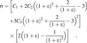
 ${\rm{\lambda }}_1 = {\rm{\lambda }}$. Since λ = 1 + ε, Eq. (14) can be rewritten as follows:
 $$\eqalignb{ {\rm{\sigma }} =\, [ {C_1 + 2C_2 ( {(1 + {\rm{\varepsilon }})^2 + {2 \over {(1 + {\rm{\varepsilon }})}} - 3} ) \cr+ 3C_3 ( {(1 + {\rm{\varepsilon }})^2 + {2 \over {(1 + {\rm{\varepsilon }})}} - 3} )^{2} } ] \cr \!\times [ {2 ( {(1 + {\rm{\varepsilon }}) - {1 \over {(1 + {\rm{\varepsilon }})^2 }}} )} ]. \cr}$$
The Yeoh model is defined by the relationship between the strain energy density and the first invariant, i.e., W–I 1. It can be expressed in terms of nominal stress (σ) and nominal strain (ε) as shown in Eq. (15).
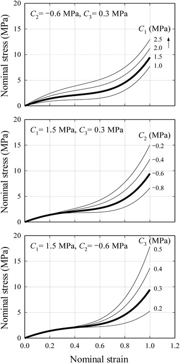
Stress–strain curves obtained by Eq. (15) are shown in Fig. 3 for three Yeoh coefficients, C 1, C 2, and C 3. The bold line in each figure indicates the stress–strain curve obtained by tentatively selected reference properties (C 1 = 1.5 MPa, C 2 = −0.6 MPa, and C 3 = 0.3 MPa). One of the three coefficients is varied, while the other two values are fixed as the reference values. In the initial stage of deformation, C 1 dominates the stress–strain curve. As the strain is increased, C 2 becomes a second influential variable, followed by C 3. Consequently, to accurately acquire C 1 and C 2, the maximum strain should be at least 0.4 (Fig. 3), whereas it should be at least 1.0 to accurately acquire C 3.
Stress–strain curves for various values of three coefficients of the Yeoh model.

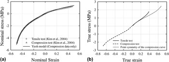
The behavior of rubber, which is usually explained by a phenomenological constitutive equation, is expressed as the relationship between the strain energy density and the strain invariants (or the principal stretches), and the constitutive equation should express well various deformation modes. If the tensile and compression tests are performed ideally, the material constants obtained from tensile and compression tests with an equivalently softened specimen must be almost identical. Figure 4(a) shows the stress–strain curves of a rubber material, SMR-CV60, obtained from the tensile and compression tests in a reference.Reference Kim, Kim, Kim, Woo and Lee21 The figure indicates that the tensile and compression data can be fitted with a set of the Yeoh coefficients, which are obtained from the compression data only. As described in Sec. II. A, the behavior in different deformation modes can be accurately predicted by the Yeoh model from data with one deformation mode. Figure 4(b) shows the true stress–strain curves of the material. The true stress–strain curve is not an odd function, whereas the true stress–strain curves of many metallic materials usually assume to be point symmetry when the Bauschinger effect is negligible. It means the tensile and compression behaviors of rubber material are not equivalent, but the Yeoh model can express these nonsymmetric behaviors with a single set of coefficients. Consequently, considering the mixed tensile, compression, and shear stress fields in the deformed indentation specimen, the Yeoh model is adequate to compare indentation properties with tensile properties.
(a) Nominal stress–strain curves of a natural rubber, SMR-CV60, obtained from tensile and compression tests. The stress–strain curve of the Yeoh model is predicted by the Yeoh coefficients of the compression data. (b) The true stress–strain curves of the tensile and compression test data. The point symmetry of the compression curve is plotted to compare the tensile and compression curves.

C. The ranges of the Yeoh coefficients
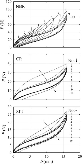
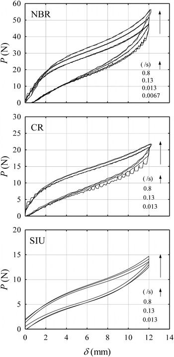
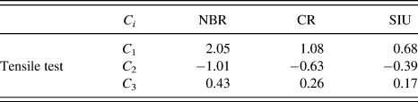
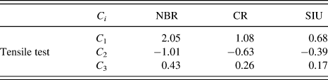
To set up the range of the three coefficients of the Yeoh model, C 1, C 2, and C 2, we carry out tensile tests for three kinds of rubbers, nitrile butadiene rubber (NBR), chloroprene rubber (CR), and silicon rubber (SIU) according to ISO37:2005. Around 7–10 cycles of loading–unloading are performed before the actual test to preclude Mullins softening effectReference Mullins22 (Fig. 5). We study then the dependence of the load–displacement curve on the strain rate using four different strain rates, 0.0067, 0.013, 0.13, and 0.8 s−1. From Fig. 6, it is confirmed that the load–displacement curves converge when the tensile strain rate is lower than 0.013/s. Hence, we define 0.013/s as the quasistatic strain rate. The corresponding material properties are regarded as quasistatic material properties. By using Eqs. (11) and (12), the relationship between W and I 1 is obtained from the tensile test data, and the Yeoh coefficients are acquired from fitting the W–I 1 curve. The ranges of the three coefficients are confined in C 1 = 0.6–2.2 MPa, C 2 = −1.1–0.0 MPa, and C 3 = 0.1–0.6 MPa. Table I shows the Yeoh coefficients of the three rubber materials. In Sec. V, we perform instrumented indentation tests with these three rubber materials. These material properties obtained from tensile tests are used as reference values.
The effect of Mullins softening on uniaxial tensile tests for three kinds of rubber materials, NBR, CR, and SIU.

The effect of strain rates on tensile tests for three kinds of rubber materials, NBR, CR, and SIU.

Yeoh coefficients of three kinds of rubber materials, NBR, CR, and SIU, obtained from tensile tests.
III. FINITE ELEMENT MODELING
A. FE modeling for spherical indentation
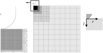
Figure 7 shows an axisymmetric finite element model. A commercial code ABAQUS14 is used to simulate spherical indentation tests for rubber materials. Since load and geometry are axisymmetric and the rubber shows incompressible behavior, four-node axisymmetric hybrid elements (CAX4H) can be used in analysis.14 To minimize the constraint caused by the bilinear shape function and to detect sufficiently small deformation, fine elements with size 1% of indenter diameter are placed around the contact surface of specimen. As the elastic modulus of indenter is relatively high compared to that of rubber, the indenter is assumed to be rigid; therefore, rigid surface14 is used. The finite element (FE) model consists of about 12,300 elements and 12,500 nodes. Contact surfaces14 are placed on both contact surfaces of specimen and indenter. Roller boundary conditions are imposed on the bottom and the axisymmetric axis of the specimen. The bottom of the indenter is a hemispherical rigid body with diameter D = 1 mm, and the upper part of the indenter is a cylindrical rigid body with radius R = 0.5 mm (Fig. 7). It should be noted that our FE model can be applied to any indenter diameter because all numerical formulas normalized by the indenter diameter make the method universally applicable irrespective of its size.Reference Lee, Kim, Lee and Nahm2, Reference Lee, Lee and Pharr23 To analyze and quantify the effects of indentation variables on the load–displacement curve, we set up the ranges for the main variables, i.e., the material constants of the Yeoh model, as described in Sec. II. C. To precisely extract the property C 3 of the Yeoh form, the maximum indentation depth, h max, is set as h max = D, which is deeper than that of our previous work.Reference Lee, Kim, Lee and Nahm2 The friction coefficient used in this study is explained in Sec. III. B.
The axisymmetric finite element model for the spherical indentation.

To investigate the size effects of the indentation specimen on the load–displacement curve for a given indenter diameter, we perform FE analyses with selected material properties (C 1 = 1.0 MPa, C 2 = −0.4 MPa, and C 3 = 0.4 MPa) in the defined property range. The height (H) and radius (W) of the cylindrical specimen are varied. In total, nine cases are applied in finite element analysis (FEA) with three ratios for H/D and W/D (24, 48, and 96). From this, we conclude that H/D = 48 and W/D = 48 are the optimal specimen size because the effect of specimen size is saturated here. The z-directional displacement at the end of the top surface can be regarded as 0. The effects of the specimen size on the indentation results with some other combinations of the coefficients are checked, and we conclude that H/D = 48 and W/D = 48 are sufficient to use as saturated dimensions in this study. It should be noted that in indentation study, 10% rule (the ratio of the indentation depth to the specimen size) is conventionally used, but it is about 2% in this study because we set h max = D, which is much smaller than the conventional value.
B. Friction coefficient
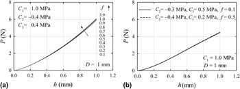
Friction forces occur at an interface where tangential and normal forces are applied. To define friction, the Coulomb friction model is generally used. The friction coefficient, f, can change depending on the state of lubrication, contamination, and materials. Kim et al.Reference Kim, Kim, Na and Lee24 have shown that the friction coefficient between structural steel and vulcanized natural rubber is affected by normal load, deformation rate, state of lubrication, and the thickness of the rubber plate. In their study, the friction coefficient was estimated at 1.6–3.9 in the case of unlubricated surfaces and 0.1–0.2 for grease lubrication. It is therefore required to quantitatively evaluate the effect of the friction coefficient on the indentation analysis. Thus, we perform FEA for various friction coefficients between indenter and rubber specimen. Figure 8(a) shows the indentation load–displacement curves for a wide variety of friction coefficients when the Yeoh coefficients are assumed to be C 1 = 1.0 MPa, C 2 = −0.4 MPa, and C 3 = 0.4 MPa. Here, h is the indentation depth, and P is the indentation load. Lee et al.Reference Lee, Kim, Lee and Nahm2 used the values of 0.09–0.13 for the friction coefficient assuming well-lubricated conditions; however, the assumption can be impractical. Figure 8(b) shows an example where two sets of material properties and friction coefficients can show almost the same P–h curve; this means that the previous methodReference Lee, Kim, Lee and Nahm2 could produce wrong material properties for unlubricated conditions. Hence, we concluded that there is no reason to consider lubrication between an indenter and a specimen, which makes this indentation testing simpler. It is therefore reasonable to suggest an updated indentation approach with properly assumed values of the normalized indentation depth h/D and the friction coefficient. As shown in Fig. 8(a), the indentation load–displacement curves converge as the friction coefficient increases, and when it is greater than 0.5, they are not affected by the friction coefficient any more. The effects of the friction on the indentation responses with other combinations of the Yeoh coefficients are tested, and 0.5 is suitable to use as a sufficiently converged friction coefficient. Hence, we select 0.5 for the friction coefficient between indenter and rubber specimen and perform static FEA by using this value. Therefore, the static indentation approach to evaluate rubber material properties can be assumed to be independent of the frictional coefficient.
(a) Indentation load–displacement curves of a rubber material (C 1 = 1.0 MPa, C 2 = −0.4 MPa, and C 3 = 0.4 MPa) with various friction coefficients. (b) Two set of material properties and friction coefficients can generate almost the same P–h curve.

IV. A NUMERICAL APPROACH TO INDENTATION TECHNIQUE FOR PROPERTY EVALUATION
A. The optimal data acquisition point
The distributions of nominal stress–strain (and W–I 1) data under the indenter are definitely complicated. To estimate rubber properties from indentation tests, it is therefore necessary to define the representative stress–strain or the representative strain energy density–first invariant corresponding to the indentation load–displacement. The detailed basis of the selection is well described in our preceding work.Reference Lee, Lee and Pharr23, Reference Lee, Kim and Lee25 Applying these indentation methodologies to the present study, we obtain the relation between (representative) W–I 1 data at a selected data acquisition point. To find the optimal data acquisition point, we investigate the distributions of W [Fig. 9(a)] and I 1 [Fig. 9(b)] along radial direction (r/D) for four l/D values; here, l is the distance from specimen surface to data acquisition depth before deformation, and r is the projected distance from axisymmetric center after deformation. When h/D = 1, the strain energy density and the first principal invariant I 1 reach a maximum at l/D = 35%. In this study, we select r/D = 0 and l/D = 35% as the optimal data acquisition point.
B. Numerical formulas for spherical indentation
The constitutive equation for the Yeoh modelReference Yeoh3, Reference Yeoh4 is expressed in terms of the strain energy density W and the first invariant I 1. Lee et al.Reference Lee, Kim, Lee and Nahm2 adopted nondimensional functions such as Eqs. (1) and (2) to map load–displacement onto W–I 1:
 $${\rm{\psi }}\, \equiv \,WhD/P\quad,$$
 $$\phi \, \equiv \,I_1\quad .$$
They indented materials up to 40% of indenter diameter (h/D = 0.4), which is the maximum depth where the effects of friction and C 3 on load–displacement curve can be neglected. For commercial vulcanized rubber, the next equations for ψ and  $\phi $ as a function of C 1, C 2, and indentation depth were obtained through FEA when C 3= 0.005 MPa as a representative constant value:
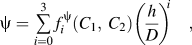 $${\rm{\psi }} = \mathop\sum\limits_{i = 0}^3 {f_i ^{\rm{\psi }} (C_1 ,\,C_2 )\left( {{h \over D}} \right)^{i} \quad,} $$
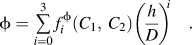 $$\phi = \mathop\sum\limits_{i = 0}^3 {f_i ^\phi (C_1 ,\,C_2 )\left( {{h \over D}} \right)^{i} }\quad .$$
Additional indentation up to h/D = 0.8 was then performed to evaluate C 3. Equation (20) represents the relationship between C 3 and P.
 $$C_3 = f^C (P) = \mathop\sum\limits_{i = 0}^2 {\left[ {\mathop\sum\limits_{j = 0}^2 {\left( {\mathop\sum\limits_{k = 0}^2 {\eta _{ijk} C_1^k } } \right)C_2^j } } \right]} \left( {{P \over {D^2 }}} \right)^{i}\quad ,$$
where ηijk are the coefficients of the polynomial function. This method is however likely to have a large error for very large deformation severely affected by the coefficient C 3. This is because to estimate large deformation well, the simultaneous variation of the three coefficients, C 1, C 2, and C 3, should be considered. In the present work, a new method to overcome this limitation is suggested.
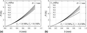
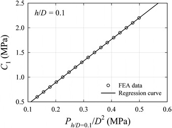
From Fig. 3, we can see that the effects of the coefficients C 2 and C 3 of Yeoh model in the initial stage of stress–strain curves are negligible. Hence, we fix C 1 and vary C 2 and C 3 one by one to identify the range in which C 1 independently affects the load–depth curve. We first fix C 1 and C 3 and vary C 2, as shown in Fig. 10(a), and then fix C 1 and C 2 and vary C 3, as shown in Fig. 10(b). Figure 10 makes it obvious that indentation load–displacement curves at h/D < 0.1 are determined by C 1 only irrespective of C 2 and C 3 values. We can thus evaluate C 1 first for h/D < 0.1 and then obtain C 2 and C 3 from triple fitting functions where h > 0.1. The relationship between indentation load  $P_{h/D\,\, = \,\,0.1} $ and C 1 is shown in Fig. 11. Based on the fitting of data in the figure, we can write
 $$\eqalignb{ C_1 = f(P_{h/D\,\, = \,\,0.1} ) = H_0 + H_1 P_{h/D\,\, = \,\,0.1} /D\,^2 \, \cr (H_0 ,\,\,H_1 ) = (0.01663\,\,{\rm{MPa}},\,\,4.3758)\quad. \cr} $$
Indentation P–h curves for the various Yeoh coefficients of (a) C 2 and (b) C 3. In each case, other coefficients are fixed as reference values.

Comparison of C 1–Ph/D = 0.1/D 2 curve and its regression curve (h/D = 0.1).

To obtain C 2 and C 3, by the same approach as Lee et al.,Reference Lee, Kim, Lee and Nahm2 we newly define normalized functions and match each load–displacement data to its equivalent W–I 1 data. In the present work, contrary to Eqs. (16) and (17), we define new normalized mapping functions as follows:
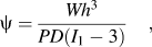 $${\rm{\psi }} = {{Wh^3 } \over {PD(I_1 - 3)}}\quad,$$
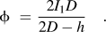 $$\phi \,\, = \,{{2I_1 D} \over {2D - h}}\quad.$$
The functions are obtained from fitting FE data for a total of 2244 cases: 17 cases for C 1 (from 0.6 to 2.2 MPa with an increment of 0.1), 12 cases for C 2 (from −1.1 to 0.0 MPa with an increment of 0.1), and 11 cases for C 3 (from 0.1 to 0.6 MPa with an increment of 0.05). The mapping functions ψ and  $\phi $can be expressed as
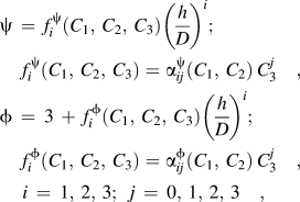 $$\eqalignb{ {\rm{\psi }} \, = \,f_i^{\rm{\psi }} (C_1 ,\,C_2 ,\,C_3 )\left( {{h \over D}} \right)^i ;\;\,\,\crf_i^{\rm{\psi }} (C_1 ,\,C_2 ,\,C_3 ) = {\rm{\alpha }}_{ij}^{\rm{\psi }} (C_1 ,\,C_2 )\,C_3^j \quad, \cr \phi \, = \,3\, + \,f_i^\phi (C_1 ,\,C_2 ,\,C_3 )\left( {{h \over D}} \right)^i ;\,\,\,\crf_i^\phi (C_1 ,\,C_2 ,\,C_3 ) = {\rm{\alpha }}_{ij}^\phi (C_1 ,\,C_2 )\,C_3^j \quad, \cr i\, = \,1,\,2,\,3;\,\,\,j\, = \,0,\,1,\,2,\,3\quad, \cr} $$
where  $f_i^{\rm{\psi }} $ and
 $f_i^{\phi} $ are the fitting coefficients with functions of C 1, C 2, and C 3. For each C 1 and C 2, the coefficients
 $\alpha _{ij}^{\rm{\psi }} $ and
 $\alpha _{ij}^\phi $ in Eq. (24) are induced from the fitting with respect to C 3. For each C 1, the next coefficients
 $\beta _{ijk}^{\rm{\psi }} $ and
 $\beta _{ijk}^\phi $ in Eq. (25) are then obtained for the variation of C 2 with the above
 $\alpha _{ij}^{\rm{\psi }} $ and
 $\alpha _{ij}^\phi $coefficients as follows:
 $$\eqalign{ {\rm{\alpha }}_{ij}^{\rm{\psi }} (C_1 ,\,C_2 ) = {\rm{\beta }}_{ijk}^{\rm{\psi }} (C_1 )\,C_2^k ;\,\,\,{\rm{\alpha }}_{ij}^\phi (C_1 ,\,C_2 ) = {\rm{\beta }}_{ijk}^\phi (C_1 )\,C_2^k\quad , \cr i = 1,\,2,\,3\,;\,\,j,k = 0,\,1,\,2,\,3\quad. \cr} $$
Finally,  ${\rm{\gamma }}_{ijkl}^{\rm{\psi }} $ and
 ${\rm{\gamma }}_{ijkl}^\phi $ are produced for the variation of C 1 with the above
 ${\rm{\beta }}_{ijk}^{\rm{\psi }} $ and
 ${\rm{\beta }}_{ijk}^\phi $coefficients as follows:
 $$\eqalignb{ {\rm{\beta }}_{ijk}^{\rm{\psi }} (C_1 ) = {\rm{\gamma }}_{ijkl}^{\rm{\psi }} C_1^l ;\,\,{\rm{\beta }}_{ijk}^\phi (C_1 ) = {\rm{\gamma }}_{ijkl}^\phi C_1^l \quad, \cr i = 1,\,2,\,3;\,\,\,j,k,l = 0,\,1,\,2,\,3\quad. \cr} $$
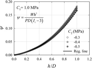
In Fig. 12 and 13, FE data for  $\psi - h/D$ and
 $\phi - h/D$ (symbols) are compared with curves generated from Eq. (24) for C 1 = 1.0 MPa and C 2= −0.3, −0.4, and −0.5 MPa. The developed fitting functions closely follow the FE results.
Comparison of regressed ψ curves with FEA data.

Comparison of regressed  $\phi $curves with FEA data.

C. Evaluation of the Yeoh properties
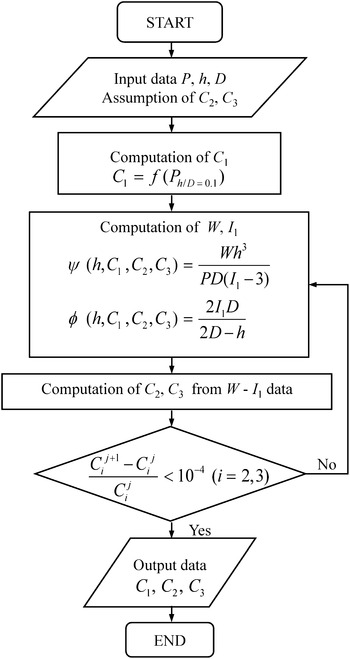
In the preceding section, the normalized functions, ψ and  $\phi $, which map the indentation load–displacement curve onto the W–I 1 curve, were established from FE data for a property range of the generally used rubber materials. The flowchart of the property evaluation program by using the normalized mapping functions is shown in Fig. 14. The detailed procedure can be described as follows. First, indentation tests are simulated and a load–displacement curve up to h/D = 1.0 is generated from FE analysis. C 2 and C 3 are initially assumed to be −0.4 and 0.4 MPa, respectively; second, C 1 is determined by substituting the load at h/D = 0.1 into Eq. (21). Using C 1, C 2, and C 3, the ψ and
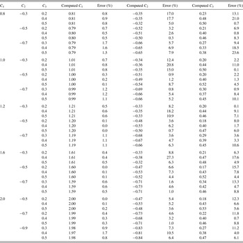
 $\phi $ functions in Eq. (24) are determined; the W–I 1 curve corresponding to the load–displacement curve is obtained from Eqs. (22) and (23). Regression of this W–I 1 curve produces updated coefficients, C 2 and C 3. These updated properties are compared with the previous ones. The process is repeated until the updated C 2 and C 3 satisfy a convergence limit. The predicted properties are compared with given material properties for 45 cases (Table II). The average errors of C 1, C 2, and C 3are 0.6%, 7.0%, and 7.6%, and the standard deviations are 0.5, 5.8, and 5.6%, respectively.
Flowchart for the determination of the Yeoh coefficients.

Comparison of computed material property values to those given.

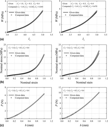
To investigate the effects of prediction errors on W–I 1 and nominal stress–strain curves, we compare W–I 1, stress–strain, and load–displacement curves for given properties with those of predicted properties, especially for the two kinds of materials having relatively large prediction errors in 45 cases (Fig. 15). The prediction errors are about 20.8% and 27.3% for C 2 and 11.0% and 17.6% for C 3. However, as we cannot distinguish the differences in the curves in Fig. 15, we may state that the quantitative errors of the properties are of secondary importance. The accuracy of the developed method should be therefore confirmed by comparisons of these three curves. From these comparisons, our new technique is highly accurate for the selected ranges of material properties of hyperelastic rubber.
Comparison of the predicted data to those given for (a) W–I 1, (b) nominal stress–nominal strain, and (c) P–h curves.

V. EXPERIMENTAL VERIFICATION OF INDENTATION TECHNIQUE FOR PROPERTY EVALUATION OF RUBBER
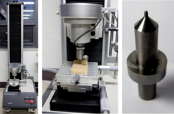
An instrumented indentation system is developed to verify the effectiveness of the indentation technique for rubber property evaluation, as shown in Fig. 16. Whereas the load cell capacity of indentation system for metallic materials is 500 kgf,Reference Lee, Kim and Lee25, Reference Lee, Lee, Hyun and Kim26 the load cell capacity of this indentation system for rubber materials is 10 kgf because lower indentation load is needed for rubber materials. The resolution of load cell is 0.15% of its capacity. A linear encoder and a digital linear variable differential transformer (LVDT) with high precision are used for the measurement of indentation depth. An AC servomotor with maximum 1.27 Nm torque precisely controls the displacement. The maximum and minimum speeds are 60 and 0.3 mm/min, respectively, so we can test materials with a wide range of strain rates. Unified spherical indenters with the tip diameter of 1 mm are used (Fig. 16), which is made of Tungsten Carbide (WC) with elastic modulus 550 GPa.
The configuration of the indentation system and the integrated indenter.

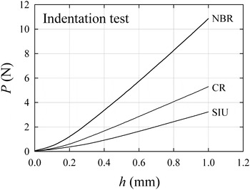
Indentation tests with the developed system are performed with three hyperelastic materials, NBR, CR, and SIU, and material properties are evaluated. After precluding the Mullins softening effect, indentation tests are performed with the same specimens as those for tensile tests. It is found that the dependence of strain rate on load–displacement curve is lower when the test speed is below 0.01 mm/s. Thus, we use 0.005 mm/s as quasistatic indentation speed. Three indentation load–displacement curves for the three materials at a speed of 0.005 mm/s are shown in Fig. 17. It should be noted that the indentation and tensile strain rates cannot be identical because their deformation modes, shapes, and distributions of stress–strain are not the same. More important thing is respective quasistatic speed that does not affect the load–displacement response. If we can control the deformation rate below the quasistatic conditions, the relative speed values between the testing methods become unimportant.
Indentation P–h curves of three kinds of rubber materials, NBR, CR, and SIU, at a quasistatic indentation speed.

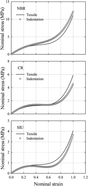
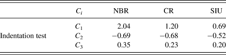
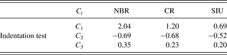
The loading part of each load–displacement curve is fed into the property evaluation program, and the material properties and its nominal stress–strain curve are evaluated. The estimated Yeoh coefficients are listed in Table III, and the nominal stress–strain curves obtained from tensile and indentation tests are compared in Fig. 18. The average gaps between C 1, C 2, and C 3 obtained by tensile and indentation tests are about 4.3%, 24.3%, and 15.7%, respectively; the maximum gap is about 30%. However, as we mentioned in Sec. IV. C, these errors are of secondary importance, and the direct comparison of the stress–strain curves are more essential to the evaluation of validity. As shown in Fig. 18, the two curves obtained from tensile and indentation tests are close up to about ε = 0.4, and they deviate from each other afterward. These deviations can be caused by a difference between tensile and indentation specimens such as the Mullins softening effect (which may still remain in the rubber material), the velocities of both tests (i.e., the effect of strain rate dependency), the accuracy of the tests (i.e., the resolutions of load cell and LVDT, the correction of the measured data including initial penetration depth in indentation), and the deviation of properties in a given material. During the tensile tests, large errors exist due to the similar factors mentioned above, so these amounts of deviations can sufficiently occur in a single material. In addition, it should be noted that real rubber materials may not be perfectly expressed by the Yeoh model or other forms with only a few material coefficients. Hence, these deviations seem quite acceptable from an engineering point of view, and moreover, we can obviously conclude that this indentation approach is highly accurate up to the engineering strain 0.4, which is a very large strain, and even up to strain 1, we can nicely predict the material behavior of rubber with only three parameters in a simple indentation test.
Comparison of indentation nominal stress–nominal strain curves to tensile nominal stress–nominal strain curves for three kinds of rubber materials, NBR, CR, and SIU.

Yeoh coefficients of three kinds of rubber materials, NBR, CR, and SIU, obtained from indentation tests.
VI. SUMMARY AND CONCLUDING REMARKS
The Yeoh model has three advantages: first, the Yeoh model using the three coefficients (C 1, C 2, and C 3) is applicable to large deformation. Second, using data in one simple deformation mode, we can predict the stress–strain behavior in other deformation modes, so that the Yeoh model can be applied to complex deformation such as indentation. Third, the strain energy density of the Yeoh model is a function of only I 1. If the strain energy density is assumed to be independent of the I 2, coefficients for rubber materials can then be obtained from one single test, e.g., uniaxial tension test. In this study, we therefore chose the Yeoh model to evaluate the material properties of hyperelastic rubber via spherical indentation. We improved then the previous numerical approach, presented by Lee et al.,Reference Lee, Kim, Lee and Nahm2 to evaluate the material properties of hyperelastic rubbers. Setting up the range of material properties in the Yeoh model and practical friction coefficient, we implemented numerical analysis with deep indentation (up to h/D = 1) to accurately obtain the coefficient C 3 that has a primary role in large deformation. We chose two normalized parameters, ψ and  $\phi $, to map indentation load–depth data onto the relationship between strain energy density–first invariant and formed the normalized functions via FEA as functions of the Yeoh coefficients and indentation depth. With these improved mapping functions, a new numerical approach was developed to evaluate material properties of hyperelastic rubber. The load–displacement curve is successfully converted to W–I 1 and stress–strain curves with average error of 0.6%, 7.0%, and 7.6%, for C 1, C 2, and C 3, respectively. The experimental verification work with our indentation system was then performed with three kinds of rubber materials. From this, we verified the validity of our developed numerical approach.
In this study, we investigated the numerical method to evaluate the static properties of hyperelastic rubber materials with spherical indentation and verified the method with quasistatic indentation experiment. As the dynamic response is another important issue in rubber materials, dynamic indentation tests considering the effect of strain rate merit further study.
ACKNOWLEDGMENT
This work was supported by the National Research Foundation of Korea (NRF) grant funded by the Korea government (MEST) (Grant No. 2009-0086135).