


Introduction
Pine Island Glacier (PIG, Fig. 1) has the largest discharge of all West Antarctic ice streams (66Gt a−1). Although the mass balance of the Pine Island drainage basin is close to zero (Reference Vaughan, Alley and BindschadlerVaughan and others, 2001), satellite observations show a significant grounding-line retreat of PIG of about 1.2 kma−1 between 1992 and 1996 (Reference RignotRignot, 1998), and thinning of the grounded terminus by up to 1.6ma−1 between 1992 and 1999 (Reference Shepherd, Wingham, Mansley and CorrShepherd and others, 2001). This thinning cannot be explained by short-term variations in accumulation and is expected to be a result of a change in the dynamics of the glacier. Whether this change is a consequence ofexternal forcing or internal feedbacks is not yet clear. An improved understanding of the controls on the flow of PIG is needed to assess the causes of the observed changes.
Horizontal surface velocities of pine island glacier derived from satellite interferometry. contour intervals are 100 m a−1below 500 m a−1, and 500 m a−1above. the thick solid lines show the two transect profiles for which the basal topography is known and to which the model is applied. the kilometre marks refer to the distance along the profiles used in figures 2–6.the dashed-dotted lines indicate the locations of the cross-profiles shown in figure 2. the thick dashed line indicates the grounding line. in grey areas no velocity observations are available, because of either missing satellite data coverage or loss of coherence.

In the main trunk of PIG, driving stresses are rather low (∼30 kPa), whereas directly behind the grounding line high driving stresses (4100 kPa) occur (Reference Vaughan, Alley and BindschadlerVaughan and others, 2001). The high driving stress and a significant deepening (approximately 500 m) of basal topography inland of the grounding line are in contrast to the low driving stresses (∼10 kPa) and flat base of the ice streams in the Siple Coast area of West Antarctica. PIG does, however, have shear margins bordering slow-moving ice, which are characteristic of other West Antarctic ice streams and suggest that resistive forces from the margins may be an important control on the flow. Ice-penetrating radar data suggest that the base is at the pressure-melting point in the main trough (Reference Vaughan, Alley and BindschadlerVaughan and others, 2001).
The aim of this study is to investigate the flow and stress regime of PIG, and in particular to evaluate the role of basal and lateral drag, and longitudinal stresses in the force balance. A special focus is given to the determination of the unknown basal friction field. A numerical model for ice-stream flow is used to calculate the flow of PIG along a flowline. The basal friction distribution is estimated by inverting observed surface velocities using a control method, which is presented in detail in this study. The control method used here is similar to that applied by Reference MacAyeal, Bindschadler and ScambosMacAyeal and others (1995) on Ice Stream E.
Flow Model
The numerical flow model used in this study calculates the horizontal flow along a flowline (x direction). It is based on a leading-order approximation of the stress equilibrium equations for ice-stream and shelf flow derived by Reference MacAyealMacAyeal (1989). The main assumption is that vertical shearing of the horizontal velocity u is negligible, which means the horizontal flow is independent of the vertical coordinate z.
The high driving stresses in the main trunk behind the grounding line (315–365 km in Fig. 3c and h, shown later) imply that here vertical shear of horizontal velocity may become important. Using the shallow-ice approximation (Reference HutterHutter, 1983), the horizontal velocity due to vertical shearing is estimated on the basis of surface slope and ice thickness. A temperature-dependent rate factor is used (Reference Paterson and BuddPaterson and Budd, 1982), and as a first approximation the vertical temperature profile is assumed to increase linearly from the mean surface air temperature ts = –22°C (Reference Giovinetto, Waters and BentleyGiovinetto and others, 1990) to Tb = 0°C at the bed. This estimated deformation velocity is in most parts well below 3% of the observed surface velocities and below 17% in the region where the high driving stresses occur (Fig. 3b and g, shown later). Furthermore, most of the deformation is expected to occur in the basal layers (perhaps with enhancement due to fabric evolution) and therefore the horizontal velocity will be more-or-less constant for most of the ice thickness. Omitting vertical shear in our model is therefore a reasonable first approximation. The one problematic area is where the high driving stresses occur (325–365 km). However, whether we take the velocity constant with depth or not is expected to have little effect on the basal drag (Reference Van der Veen and WhillansVan der Veen and Whillans, 1989; Reference Whillans, Chen, vander Veen and HughesWhillans and others, 1989). We will return to this assumption of no vertical shear in the discussion, because a detailed analysis would require knowledge of the lateral and basal traction, which we do not have at this stage but which will be available after our analysis.
In this study, only horizontal flow u along a flowline is considered (x direction), and we assume there is no flow in the transverse direction to the ice stream (y direction). The force balance in a profile along the flowline is then given by

where h is the ice thickness,
 is the longitudinal stress deviator defined as the difference between the longitudinal stress and hydrostatic pressure, τxy
is the lateral shear stress, τb the shear traction at the bed, p the density of ice, g the acceleration due to gravity and s the surface elevation. Thus the driving stress τd on the righthand side of Equation (1) is balanced by gradients in longitudinal stress and resistive forces at the glacier bed and at the margins. Using Glen’s flow law (Reference GlenGlen, 1955) and defining an effective viscosity
 , where n is the flow-law exponent, A the rate factor and
the effective strain rate, σ’x
can be written as
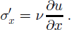
The effective strain rate is calculated assuming no vertical and lateral shearing of the horizontal velocity, which leaves the longitudinal variation alone and leads to an underestimation of
 in places where the longitudinal strain rates are close to zero.
The basal shear traction of the ice stream is assumed to be linearly related to the basal velocity ub (Reference MacAyealMacAyeal, 1989):

where β 2 is the basal friction coefficient. A realistic relationship between τb and ub is likely to be non-linear, but the details of such non-linearities are unknown (Reference RaymondRaymond, 1996). Therefore the most simple case of a linear relation is considered here. At the base of the ice shelf, basal traction τb is zero which is included in the model by setting β = 0.
Because resistance to flow from side shear is recognized to be important in the force budget of ice streams (Reference Echelmeyer, Harrison, Larsen and MitchellEchelmeyer and others, 1994), lateral drag is included in the model using a parameterization suggested by Reference Van der Veen and WhillansVan der Veen and Whillans (1996). Integration of Equation (1) over the width of the ice stream, assuming constant ice thickness across the channel of half-width W, gives

where τs is the lateral stress. Considering lateral drag independent of basal drag and linking the lateral shear stress to the transverse shear strain rate with Glen’s flow law, τs can be expressed in terms of the width-averaged velocity u by

An alternative way of including the lateral drag is to calculate the term ∂hτxy/∂y in Equation (1) directly from the observed two-dimensional horizontal surface velocity field, which has been done in some additional model runs. Unless noted differently the parameterization of Reference Van der Veen and WhillansVan der Veen and Whillans (1996) is used.
Assuming no spreading at the sides and no lateral variation of u, the boundary condition at the shelf front derives from the force balance between ice and displaced ocean water (Reference PatersonPaterson, 1994, p. 296).
Model equation and solution technique
Substituting
and τs into Equation (4) gives the final model equation for the width-averaged horizontal velocity

The lateral drag (second term on lefthand side) is linearized in
 by defining
 . To simplify the notation below, the width-averaged horizontal velocity is denoted by u instead of
. The model equation (6) is solved numerically using the finite-difference method and iterating for the effective viscosity ν and γ. Approximating the x derivatives by centred differences, the discretized model equation can be written as a linear system of equations in the unknown surface velocity u
j:

where i and j denote the gridpoint number, a is a tridiagonal nxn matrix and is a function of ν and γ. For each iteration step, this linear system of equations is solved for ui using ν and γ calculated from the velocities of the previous iteration step.
Control Method
The basal friction coefficient f2 in Equation (6) is an unknown parameter in our numerical model for ice-stream flow. We determine it here by inverting observed surface velocities using a control method similar to that used by Reference MacAyealMacAyeal (1993) and Reference MacAyeal, Bindschadler and ScambosMacAyeal and others (1995). For details of this method we refer to applications in oceanography (Reference ThackerThacker, 1988; Reference Thacker and LongThacker and Long, 1988; Reference SchlitzerSchlitzer, 1993).
The control method is designed to find the set of unknown model parameters
 which when substituted into the model equation produces the best fit between modelled
 and observed
 quantities. The misfit is measured by a cost function J, which is taken here as

where
 is a weighting factor (ideally taken as the observational error). Searching for the set of model parameters pi
that gives the best fit is the same as minimizing j while ensuring that the model equations are satisfied. This is done by the method of Lagrange multipliers (Reference ThackerThacker, 1988). The model equation (6) written in the finite-difference form for each gridpoint i is given by

We now introduce the Lagrangian l by

where Λ = (λ1; :::; λn) are the Lagrange multipliers. The importance of the Lagrangian is that the minimum of the cost function is found when the gradient of l in respect to λ i,qj and pj vanishes:


On differentiation with respect to λ
i, Equation (11) recovers the model equation. Seeking for the minimum of j is now equivalent to finding a model solution that satisfies the model equation (θ) and the adjoint model equations (12) and (13). Equation (12) represents a system of n linear equations in the n unknown Lagrange multipliers Λ = (λ1; . . . ; λn) from which A can be calculated. Introducing Λ into Equation (13) allows us to calculate the gradient of l with respect to the model parameters pj
given by
 . It is down this gradient that a new improved guess for the model parameters p is determined by applying a descent algorithm (Polak–Ribiere method; Reference Press, Flannery, Teukolsky and VetterlingPress and others, 1989, p. 303).
In this study, the observed surface flow field is inverted for the basal friction coefficient f. Thus, the unknown model parameters p are given by the basal friction coefficient fi at each gridpoint i = 1; . . . ; m and q d and q are given by the observed and modelled horizontal surface velocities
 and ui, respectively. The weighting constant σq
is taken equal to the observation error of the surface velocity (σu).
The control method algorithm can be summarized as follows. First, the model parameters fj are initialized by a first arbitrary guess βinitial. The following steps are then repeated until the minimum of J is reached or j is reduced to a value that is consistent with the error in the measurements. The cost function j is evaluated and calculated by solving the adjoint equations (12) and (13). Using this gradient ∇J and a conjugate gradient method, a new improved set of model parameters βj is determined for input to the ice-stream model.
In our case, the discretized version of the model equation is linear in ui (Equations (6) and (7)) and the adjoint equation (12) can be written as

where the * denotes the transpose of a matrix. The matrix aj k is already known from solving the forward model (Equation (7)); thus the determination of the λi does not need any extra effort.
Observations and Model Setting
Velocities and geometry
The surface velocity field for PIG is known from satellite radar interferometry from European Remote-sensing Satellite (ERS) synthetic aperture radar (SAR) data recorded between 1994 and 1996 (Reference Shepherd, Wingham, Mansley and CorrShepherd and others, 2001). There is a gap in the coverage of the interferometric data on the right-hand side of the main trough (Fig. 1). The surface and basal topography is only known on two transect profiles (A and B) from airborne radar sounding (Reference Corr, Doake, Jenkins and VaughanCorr and others, 2001; Reference Vaughan, Alley and BindschadlerVaughan and others, 2001). Because the basal topography is not known outside of these two profiles, we decided to perform the model calculations along the two profiles. Using a transect model for stream flow requires that the profile is approximately along the direction of glacier flow in the lower 200 km of interest. This is the case for profile A, but, because the glacier turns slightly to the right (in the flow direction) in the fast-flowing part, profile B comes close to the ice-stream margin, resulting in a surface velocity depression along this profile (Fig. 1; Fig. 3g, shown later).
Model setting
The horizontal grid size δx equals 5 km and the flow-law exponent is set to n = 3 (Reference PatersonPaterson, 1994, p. 85). Unless otherwise specified, a rate factor a = 4.9 6 10–25 s−1 Pa−3 corresponding to an ice temperature of t = –10°C is used (Reference PatersonPaterson, 1994, p.97), and is assumed to be constant over the whole model domain. The flow model calculates the width- and depth-averaged velocity and stress fields for a glacier that flows down a rectangular channel of half-width w and thickness h, which both vary along x. Instead of observed width-averaged velocities, we used the observed velocities along the profiles and assumed that they are representative for the width-averaged flow. The four velocity cross-profiles shown in Figure 2 support this assumption. The differences between the width-averaged velocities and the velocities at the locations of profiles A and B are in general 5 ±10%.
Surface velocities in the cross-profiles 1–4 marked in Figure 1. The crossings with profiles A and B are marked, and the mean velocities over the stream width are shown as dashed-dotted lines.

Glacier width
The width of PIG along its whole length is not well defined, and a simplified width distribution along the transect is estimated on the basis of the interferometrically derived velocity field (Fig. 1). A half-width of w = 20 km is chosen for the ice shelf, w = 16 km for the ice stream in the main trunk and w = 30 km further up-glacier. I n the numerical model, the choice of w(x) only affects the parameterization of the lateral drag (Equation (6)).
Shear softening
The parameterization for lateral drag used here is based on the assumption that τs is independent of the basal drag and simply linked to the transverse shear strain rate. Thus, the resistance at the margin is expected to be overestimated. Lateral drag may additionally be reduced by softening of the ice in the shear margins due to strain heating and intense crevassing (Reference Echelmeyer, Harrison, Larsen and MitchellEchelmeyer and others, 1994). We account for shear softening by introducing an optional shear softening factor fsoft in the parameterization of the lateral drag by

In the ice shelfβ2 = 0 and the driving stress is balanced by lateral drag and longitudinal stress gradients. The parameterization for τs turns out to be unrealistic for the ice-shelf region because there the calculated lateral drag partly exceeds the driving stress. This is mainly a result of the high flow velocities and very low driving stresses in the shelf part. To avoid unrealistically high lateral stresses and to obtain ice-shelf velocities of the right order of magnitude, shear softening for the shelf ice is assumed. This study focuses on the flow and stress regime in the ice stream, which is found to be insensitive to the chosen softening factors and boundary conditions in the ice-shelf part.
Initial guess of β2
The control method requires an initial guess for the model parameter β2, which in this study is chosen generally as the explicit solution β 2 of the model equation (6) neglecting the longitudinal stress gradients. To check the sensitivity of our final results to the initial guess, additional inversions with constant initial β 2 of 2.5 6 109 and 10.0 6 109 P a sm1 , respectively, are calculated.
Data uncertainty
The error estimate for the observed surface velocity σu =15 m a−1 (personal communication from A. Shepherd, 2002) includes random measurement errors and interpolation errors. In a 30 km section of profile A, the surface velocities are unknown (Fig. 1). Based on the known velocity field in the surrounding areas and along the other transect, we do not expect any unusual changes in the velocity field, and therefore the velocities are linearly interpolated. To account for the additional uncertainty in this region, a larger error of σu = 60 ma−1 is used.
Acceptance of fit
A fit between model results and observations, and the associated model parameters, is accepted when the cost function j is reduced to a value J a consistent with the measurement error in the observations. Assuming that the observation error is a random variable and has a Gaussian probability distribution, our misfit j is closely related to a À2 distribution with m- 1 degrees of freedom (Reference MenkeMenke, 1989, p. 32; Reference MacAyeal, Bindschadler and ScambosMacAyeal and others, 1995), where m is the number of observed velocities on gridpoints. We accept an inversion run if j is reduced below the bound J a which is chosen as the level of À2 that corresponds to a 10% probability of occurrence (Reference MenkeMenke, 1989). This means that a further improvement of the fit could not be differentiated from the effect of random measurement errors. In our case of 50 degrees of freedom, the value of acceptance is Ja = 63.17 (Reference Mendenhall, Wackerly and ScheafferMendenhall and others, 1989). Whenever j falls below this value of 63.17, the random error in observation could account for a misfit greater than j with a probability of 10%.
Model Results
The model calculations and interpretations are focused on the region where the flow is expected to be dominated by basal sliding, that is, the main trunk and the grounding-line region (200–380km).
Reference inversion
Various runs of the control algorithm were performed for profiles A and B with different parameter assumptions. The results of the reference inversions A and B are shown in Figure 3. Figure 3c and h show each term of our balance equation (6) separately. For the calculated stress regime, three different sections can be identified along the transect for both profiles. In the grounding-line zone and immediately behind (365– 385 km, an area often called the ice plain), the resistive stresses from the base and the sides, and the longitudinal stress gradients are all of the same order of magnitude. In the region behind (315–365 km), the high driving stress τd (up to 160 kPa), due to a significant increase in surface slope, is mainly balanced by basal drag τb. Although lateral drag and longitudinal stress gradients reach the highest values in this region, they are small compared to τb. For profile B, the high basal shear traction could be interpreted as a consequence of the local velocity minimum in the profile, which is itself due to the fact that the profile does not exactly follow the flowline and approaches the margin closely. However, for profile A, which follows the true direction of flow, the surface velocity increase is monotonic towards the grounding line, and the stress regime is very similar.
Profile a: (a) surface and bed topography; (b) calculated and observed surface velocities (crosses) and estimated vertical shear of the horizontal velocity (dots) using the shallow-ice approximation; (c) driving stress and calculated basal drag τb, lateral drag h/wτs and longitudinal stress gradients; (d) calculated basal friction coefficient β2; and (e) difference between modelled and observed velocities shown with the corresponding measurement error σu (dashed lines). the dotted line here and in the remaining figures indicates the grounding line. profile b: (f) as for (a); (g) as for (b); (h) as for (c); (i) as for (d); (j) as for (e).

In the main trunk (200–315 km), where the surface slope is small and smooth, the driving stress is low (10–40 kPa) and is mainly balanced by lateral and basal drag, and longitudinal stress gradients are rather small (Fig. 3c and h). Similar sections can be identified for the basal friction coefficient /32 (Fig. 3d and i). For profile A, there is no significant difference in the value of /32 between the steep and flat parts of the main trough, a result which is not obvious considering the huge differences in τb and driving stress. For profile B, /32 is slightly higher in the zone of high τb. This might be due to the velocity reduction where the profile comes too close to the margin.
Additional model runs
To check the sensitivity of the model inversion and parameter assumptions, additional model runs and inversions have been calculated by varying the rate factor a the width w of the ice stream, the shear softening factor fsoft at the margins and the
Sensitivity to the initial choice of (32)
To check the influence of the initial guess for the model parameter β 2 on the final β 2 or on τb, additional inversions with a constant initial β 2 of 2.5 6 109 and 10.0 6 109 Pas m–1, respectively, are calculated (Fig. 4). The resulting β 2 and τb distributions are very similar, which suggests that the inversion method used is not significantly affected by the choice of the initial guess for β 2.
Calculated basal traction relative to the driving stress along profile a, shown for the reference inversion (crosses), an inversion with a constant initial β2=10×109 pa s m1 (dots) and with a rate factor corresponding to –20°c (triangles). the numbers in the legend here and in figures 5 and 6 indicate the inversion run number from table 1.

Inversion for β and the basal topography
A run in which the model is inverted for the basal topography b (in addition to β) has also been performed. The idea is that b is not well constrained by measurements and is therefore taken as an additional unknown model parameter. The observed basal topography bd is used as initial guess for b. An additional term Jb, which measures the misfit between observed and calculated bed elevation, is added to the total cost function j which is now given by

where σb is the measurement error of the basal elevation which is here set to 10 m. The gradient of l is then given by vj=(∂l/∂0j,∂l/∂bj).
In our case, the contribution of J b turns out to be rather small in comparison to ju, and the final β and τb distributions are very similar to the reference inversion performed for β only (Table 1). Thus, changes of b in the range of the measurement error do not significantly affect the inverted β
List ofthe performed inversions that were accepted (Jfell below 63.17).The mean values (overbar) along the transect and their standard deviations (σ) are listed for the basal drag
 lateral drag
 in kPa and the basalfriction coefficient
 in Pa s m1

Lateral drag derived from the observed two-dimensional velocity field
Model runs for both profiles have been performed which use an alternative way of including lateral drag in our ice-stream model. Using Glen’s flow law, τxy is approximated as

Using this expression the lateral shear stress term ∂hτxy/∂y in Equation (1) can be explicitly calculated from the observed two-dimensional surface velocity field along the two profiles. The lateral drag calculated from the original velocity data is rather noisy because it is found from the second derivative of the velocity across the ice stream. Therefore, additional model inversions were performed using differently smoothed surface velocity fields to represent lateral drag (Table 1, Nos. 15–18.). The resulting lateral drag and the inverted basal drag for profile A are shown in Figure 6 and confirm the general stress pattern found above. The large differences of the basal drag relative to the driving stress behind the grounding line are mainly due to differences in the lateral drag.
Calculated basal traction relative to the driving stress along profile a, shown for the reference inversion (crosses), an inversion with a constant half width w=20km (dots) and with no lateral drag (τs =0) (triangles).

(a) Calculated basal traction relative to the driving stress, and (b) lateral drag along profile A, shown for the reference inversion (crosses) and two inversions using a lateral drag calculated directly from the two-dimensional surface velocity field for two differently smoothed versions. The dashed line indicates the driving stress. initial guess for β2 (Figs 4 and 5). Furthermore, inversion runs were performed with a model which uses calculated lateral drag determined directly from the observed two-dimensional surface velocity field (Fig. 6). An overview of the additional inversion runs is given in Table 1. In general, the stress regime looks very similar to the reference inversion discussed above. Where the driving stress is low, the effect of changes in width, rate factor a or shear softening on the stress distribution is significant in relation to τd. In the region of high surface velocities (x > 200 km), β2 is not very sensitive to variations in the parameters and is rather low. This indicates that a small change in β2 could affect the flow significantly.

Discussion
The control method used to invert for /3 (and therefore τb), is based on the assumption that the flow model is correct. Our numerical flow model is, however, an approximation and therefore its limitations have to be taken into account. The main trunk (200–365 km) and the grounding-line region (365–385 km) of PIG are characterized by both low driving stress and basal traction. Here we are confident that the model assumption of zero vertical shear is legitimate. The area upstream of the grounding line (315–365 km) is characterized by both high driving stress (150 kPa) and basal traction.
The assumption that the velocity is constant with depth will overestimate the importance of lateral drag and longitudinal stress gradients, simply because horizontal velocity gradients are smaller at depth if deformation is important. This means that our calculated basal drag will be underestimated. Accounting for the depth variation in velocity would increase the importance of basal drag but not significantly alter the conclusion that the basal drag is the main resistance to flow in this region of high driving stress.
Our a priori analysis indicated that significant vertical shear may occur in this area (based on the driving-stress consideration alone). Because we can now estimate all stress components, the validity of our a priori assumption for this area can be checked. I n a similar manner to Reference MacAyeal, Bindschadler and ScambosMacAyeal and others (1995), we compare basal traction (as opposed to driving stress) to the stress necessary to obtain the observed surface velocity by vertical shear alone. Our results indicate that basal traction is close to the driving stress in this area (Fig. 3). Our previous a priori analysis (Flow model section) is therefore supported by model results, and detailed modelling (full stress regime) is required for this area of PIG.
In the parameterization of Reference Van der Veen and WhillansVan der Veen and Whillans (1996), the resistance from the sides is expected to be overestimated, which is clearly indicated in the ice-shelf part by the fact that the calculated lateral drag exceeds the driving stress. Shear softening would also reduce the resistance from the sides. Additionally, lateral and basal drag are considered independently, which is appropriate if either lateral or basal drag balances most of the driving stress, but may be less realistic in regions where both are equally important.
There is no significant difference in the value of /32 between the steep and flat parts of the main trough, although τb is very different. Accepting our assumptions for the model and the relation at the basal boundary, the constant value ofβ2 could be interpreted to mean that the slip properties at the bed–ice interface are very similar. This suggests that the peak in basal traction τb is a consequence of the high driving stress in the region behind the grounding line. The low values of β 2 in the grounding-line region are consistent with a region of light grounding as suggested for the ice plain (Reference Corr, Doake, Jenkins and VaughanCorr and others, 2001). The dynamics of the ice plain may therefore be significantly affected by a thinning in the region of the grounding line or ice shelf, as observed in the last few years (Reference Shepherd, Wingham, Mansley and CorrShepherd and others, 2001).
Conclusions
By the use of a simple ice-stream model, a control method has been successfully applied to determine the basal friction distribution τb along the transect of PIG from observed surface velocities. The high driving stress up-glacier from the grounding-line region is dominantly balanced by basal friction, which reaches values up to 150 kPa. In the main trough further up-glacier and in the grounding-line region, lateral drag and longitudinal stresses also become important.
The control method allows us to invert for other unknown or poorly constrained model parameters, as demonstrated for the basal topography, or to include additional or alternative observational constraints. The thinning rate of the surface ∂s/∂t can be measured by remote-sensing techniques with high accuracy (Reference Shepherd, Wingham, Mansley and CorrShepherd and others, 2001) and could easily be included as constraint in the control algorithm by adding the misfit between its observed and modelled value in the cost function. However, it would also require the incorporation and knowledge of the basal geometry across the channel.
The control method hinges on the use of a numerical flow model. The main model assumption of no vertical shear of the horizontal velocity is found to be doubtful in the region of the driving-stress peak. Further, the parameterization of the lateral drag oversimplifies the resistance from the sides in the main trough and in the grounding-line region. An improved understanding of the stress regime and dynamics of PIG therefore requires the use of a flow model that incorporates vertical shear of the horizontal velocity and considers the flow in both horizontal dimensions, but this would require detailed knowledge of basal topography outside profiles A and B.
Acknowledgements
We thank A. Shepherd from University College London for providing the velocity data, and the British Antarctic Survey for allowing us to use the basal topography data. We further thank S. Coles for statistical support. C.J. van der Veen, C. Raymond and two anonymous reviewers made very useful comments that resulted in much improved manuscript. This work was supported by the grant NER/A/S/2000/00419 from U. K. Natural Environment Research Council, and the Centre for Polar Observation and Modelling.



