







1. Introduction
Surface roughness is prevalent in many practical flows. Examples include flow through rough pipes (Allen et al. Reference Allen, Shockling, Kunkel and Smits2007), flow past bio-fouled ship hulls (Utama et al. Reference Utama, Nugroho, Yusuf, Prasetyo, Hakim, Suastika, Ganapathisubramani, Hutchins and Monty2021) and flow over vegetation canopies (Brunet Reference Brunet2020). It is well known that a hydrodynamically rough surface experiences an increased level of drag relative to a smooth surface at matched flow conditions (Moody Reference Moody1944), and that practical surfaces often exhibit irregular roughness across a wide range of length scales, e.g. turbine-blade roughness (Barros & Christensen Reference Barros and Christensen2014), machined surfaces (Thakkar, Busse & Sandham Reference Thakkar, Busse and Sandham2016) and additively manufactured parts (Townsend et al. Reference Townsend, Senin, Blunt, Leach and Taylor2016). Yet predicting the drag penalty of irregular, multi-scale roughness remains an elusive goal and continues to be a focal point of research (Flack Reference Flack2018; Chung et al. Reference Chung, Hutchins, Schultz and Flack2021).
In practice, the drag penalty due to surface roughness is described using a single parameter: the Nikuradse (Reference Nikuradse1933) sand-grain roughness,  $k_{s}$. However,
 $k_{s}$ cannot be derived from any direct measure of roughness, e.g. using digital data obtained from a surface scan. Instead, an equivalent value of
 $k_{s}$ must be assigned to a particular surface by exposing it to a range of known flow conditions and then relating measurements of the Hama (Reference Hama1954) roughness function
 $\Delta U^{+}\equiv \Delta U/u_{\tau }$, or the skin-friction coefficient
 $C_{f}\equiv \tau _{w}/(\frac {1}{2}\rho U_{b}^{2})$, to the Nikuradse (Reference Nikuradse1933) sand-grain data. Here,
 $\Delta U^{+}$ is the downward shift of the inner-scaled mean streamwise velocity profile in the logarithmic (log) layer, relative to the smooth-wall profile at matched flow conditions, and
 $u_{\tau }\equiv \sqrt {\tau _{w}/\rho }$ is the friction velocity, where
 $\tau _{w}$ is the wall shear stress,
 $\rho$ is the density, and
 $U_{b}$ is the streamwise bulk velocity. To express
 $k_{s}$ in terms of some measure for the physical roughness height, say
 $k$, a scaling factor
 $C=k_{s}/k$ can be determined by collapsing the measured values of
 $\Delta U^{+}$ onto Nikuradse's fully rough asymptote,
 $\Delta U_{FR}^{+}(k_{s}^{+})=\kappa ^{-1}\log k_{s}^{+} +A-8.5$, where subscript
 $FR$ denotes fully rough conditions,
 $\kappa$ is the von Kármán constant,
 $k_{s}^{+}\equiv k_{s} u_{\tau }/\nu$ is the viscous-scaled sand-grain roughness, and
 $A$ is the smooth-wall intercept. However, the scaling factor
 $C=k_{s}/k$ is surface-specific and must be determined for each type of roughness, e.g. virtual sandpaper roughness (Yuan & Piomelli Reference Yuan and Piomelli2014), egg-carton roughness (Chan et al. Reference Chan, MacDonald, Chung, Hutchins and Ooi2015), tube-worm roughness (Monty et al. Reference Monty, Dogan, Hanson, Scardino, Ganapathisubramani and Hutchins2016), grit-blasted roughness (Thakkar, Busse & Sandham Reference Thakkar, Busse and Sandham2018), irregular near-Gaussian roughness (Jelly & Busse Reference Jelly and Busse2019b), orange-peel roughness (Nugroho et al. Reference Nugroho, Monty, Utama, Ganapathisubramani and Hutchins2021) or industrial grade sandpaper roughness (Berghout et al. Reference Berghout, Bullee, Fuchs, Scharnowski, Kähler, Chung, Lohse and Huisman2021). Models that reliably predict
 $k_{s}/k$ (or
 $\Delta U^{+}$) based solely on key topographical parameters are therefore of great value.
Whilst the ultimate goal for roughness research is to produce a universal model that correlates key topographical parameters to  $k_{s}/k$ (or
 $\Delta U^{+}$ for transitionally rough flows), a complete exploration of the parameter space that defines the ‘roughness problem’ is simply not feasible. To overcome this challenge, it is widely accepted that a minimal set of key topographical parameters must first be identified (Flack Reference Flack2018; Chung et al. Reference Chung, Hutchins, Schultz and Flack2021), which can then be used to develop predictive models for
 $k_{s}/k$ or
 $\Delta U^{+}$. Eight predictive models for
 $k_{s}/k$ and
 $\Delta U^{+}$ proposed in past work are listed in table 1. Despite their variety, the models share three common topographical parameters. These include: (i) a measure of the physical roughness height, e.g. the mean absolute height
 $S_{a}$, the root-mean-square (r.m.s.) height
 $S_{q}$, or the mean peak-to-valley height
 $S_{z,5\times 5}$; (ii) the skewness of the height distribution
 $Ssk$; and (iii) the streamwise effective slope
 $ES_{x}$. The latter quantity is defined as
 $ES_{x}={A}^{-1}\int _{A}|{\partial h(x,y)}/{\partial x}|\,\textrm {d}A$ (where
 $h(x,y)$ is the roughness height distribution, and
 $A$ is the planform area of the surface), and is related to frontal solidity through the formula
 $\textstyle \lambda _{x}\equiv \frac {1}{2}ES_{x}$ (see MacDonald et al. (Reference MacDonald, Chan, Chung, Hutchins and Ooi2016) for details). Although models based on parameters (i)–(iii) have shown promise in predicting the roughness drag penalty (Forooghi et al. Reference Forooghi, Stroh, Magagnato, Jakirlic and Frohnapfel2017), a truly universal correlation will likely depend on additional topographical parameters related to other surface properties such as directionality or anisotropy.
Predictive models for  $k_{s}/k$ and
 $\Delta U^{+}$ based on topographical parameters, including: generalised Sigal–Danberg parameter
 $\varLambda _{s}=(S/S_{f})(S_{f}/S_{s})^{-1.6}$ (where
 $S$ is the planform area of the corresponding smooth surface,
 $S_{f}$ is the total projected frontal area of all the roughness elements, and
 $S_{s}$ is the total area of all roughness elements wetted by the flow
 $S$);
 $n$th spectral moment
 $m_{n}=\int _{0}^{\infty }\kappa _{}^{n}E_{hh}\,{\rm d}\kappa _{}$ (where
 $E_{hh}$ is the spectrum of surface elevation, and
 $\kappa _{}$ is an in-plane wavenumber); r.m.s. forward-facing surface angle
 $\alpha _{rms}=\sqrt {n_{f}^{-1}\sum _{j=1}^{n_{f}}\alpha ^{2}_{j}}$ (where
 $n_{f}$ is the total number of forward-facing roughness elements, the local forward-facing surface angle is
 $\alpha _{j}=\tan ^{-1}(\Delta s^{-1}[h_{j+1}-h_{j}])$, and
 $\Delta s$ is the streamwise spacing of the roughness elements); mean absolute roughness height
 $S_{a}={A^{-1}\iint |h(x,y)|\,{\rm d} A}$; r.m.s. roughness height
 $S_{q}=\sqrt {{A^{-1}\iint h(x,y)^{2}\,{\rm d} A}}$; skewness
 $Ssk=A^{-1}{S_{q}^{-3}}\iint h(x,y)^{3}\,{\rm d} A$; kurtosis
 $Sku=A^{-1}{S_{q}^{-4}}\iint h(x,y)^{4}\,{\rm d} A$; streamwise effective slope
 $ES_{x}={A}^{-1}\int _{A}|{\partial h(x,y)}/{\partial x}|\,\textrm {d}A$; and streamwise correlation length based on a 0.2 cutoff criterion,
 $L_{x,cor}$. Note that
 $A$ is the planform area of the height map
 $h(x,y)$.

Whilst the drag behaviours of highly directional two-dimensional surfaces have been studied extensively, e.g. streamwise-aligned riblets (Gatti et al. Reference Gatti, von Deyn, Forooghi and Frohnapfel2020; Modesti et al. Reference Modesti, Endrikat, Hutchins and Chung2021), spanwise-aligned bars (Volino, Schultz & Flack Reference Volino, Schultz and Flack2009; Krogstad & Efros Reference Krogstad and Efros2012) and spanwise-alternating rough-to-smooth surfaces (Bakhuis et al. Reference Bakhuis, Ezeta, Berghout, Bullee, Tai, Chung, Verzicco, Lohse, Huisman and Sun2020; Wangsawijaya et al. Reference Wangsawijaya, Baidya, Chung, Marusic and Hutchins2020), systematic studies of surface anisotropy in the context of irregular, three-dimensional roughness remain scarce. One exception to this trend is the work by Busse & Jelly (Reference Busse and Jelly2020), which demonstrated that irregular roughness with spanwise-elongated features induces an over 200 % increase in  $\Delta U^{+}$, relative to roughness with streamwise-elongated features in fully developed turbulent channel flow. In that work, the level of surface anisotropy was quantified using the surface anisotropy ratio (SAR) parameter, which was defined as
 $\textrm {SAR}\equiv L_{x,cor}/L_{y,cor}$, where
 $L_{x,cor}$ and
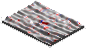
 $L_{y,cor}$ are the streamwise and spanwise correlation lengths based on a 0.2 cutoff criterion (see Thakkar et al. (Reference Thakkar, Busse and Sandham2016) for details). Yet the sensitivity of wall drag with respect to the SAR parameter or other measures of surface anisotropy cannot be predicted using any combination of the topographical parameters included in table 1. This shortcoming is illustrated by the three roughness topographies shown in figure 1, which, based on their mean peak-to-valley height, skewness and streamwise effective slope, are identical in the statistical sense – despite showing obvious differences along the spanwise (
 $y$) direction. Hence further consideration of directional topographical parameters is required to predict the drag penalty of anisotropic surface roughness.
Irregular surface roughness with identical mean peak-to-valley height  $S_{z,5\times 5}/\delta =1/6$, skewness
 $Ssk\approx 0$ and
 $ES_{x}\approx 0.35$, but differing
 $ES_{y}$. (a) Isotropic surface with
 $ES_{y}/ES_{x}=1$. (b) Spanwise-elongated roughness with
 $ES_{y}/ES_{x}\approx 0.63$. (c) Spanwise-elongated roughness with
 $ES_{y}/ES_{x}\approx 0.29$. Each surface is shown on a
 $(2\times 2)/\delta$ tile, where
 $\delta$ is the mean channel half-height.

As a first step, spanwise effective slope  $ES_{y}$ can be considered, which, in analogy to
 $ES_{x}$, is defined as the mean absolute spanwise slope of the height distribution,
 $ES_{y}\equiv {A}^{-1}\int _{A}|{\partial h(x,y)}/{\partial y}|\,\textrm {d}A$, and is related to ‘lateral’ solidity through the formula
 $\varLambda _{y}\equiv \frac {1}{2}ES_{y}$. The degree of surface anisotropy can then be inferred from the ratio of spanwise effective slope to streamwise effective slope, i.e. surfaces with
 $ES_{y}/ES_{x}=1$ are isotropic (figure 1a), surfaces with
 $ES_{y}/ES_{x}<1$ are spanwise-elongated (figures 1b,c), and surfaces with
 $ES_{y}/ES_{x}>1$ are streamwise-elongated. The limiting cases are streamwise homogeneous roughness with
 $ES_{x}=0$ and
 $ES_{y}>0$, i.e. two-dimensional riblet-like surfaces with
 $ES_{y}/ES_{x}\rightarrow \infty$, and spanwise homogeneous roughness with
 $ES_{x}>0$ and
 $ES_{y}=0$, i.e. two-dimensional spanwise bar-like surfaces with
 $ES_{y}/ES_{x}\rightarrow 0$.
Whilst systematic studies of irregular anisotropic roughness ( $ES_{y}/ES_{x}\neq 1$) remain scarce, the drag penalty of isotropic surface roughness (
 $ES_{y}/ES_{x}=1$) has been studied for various regular (Bhaganagar, Kim & Coleman Reference Bhaganagar, Kim and Coleman2004; Coceal et al. Reference Coceal, Thomas, Castro and Belcher2006; Chan et al. Reference Chan, MacDonald, Chung, Hutchins and Ooi2015; Seddighi et al. Reference Seddighi, He, Pokrajac, O'Donoghue and Vardy2015; Ma et al. Reference Ma, Xu, Sung and Huang2020) and irregular (De Marchis et al. Reference De Marchis, Saccone, Milici and Napoli2020; Flack, Schultz & Barros Reference Flack, Schultz and Barros2020; Ma, Alamé & Mahesh Reference Ma, Alamé and Mahesh2021; Nugroho et al. Reference Nugroho, Monty, Utama, Ganapathisubramani and Hutchins2021; Portela, Busse & Sandham Reference Portela, Busse and Sandham2021) topographies. The current lack of studies on turbulent flow over surface roughness with systematically varied
 $ES_{x}$ and
 $ES_{y}$ is conveyed in figure 2, where data points from the present study and past work are plotted on the
 $ES_{x}$–
 $ES_{y}$ plane. Relative to the combinations of
 $ES_{x}$ and
 $ES_{y}$ considered in the present study (shown as filled black circles in figure 2), most past data appear scattered, and few systematic patterns can be discerned. An exception to this trend is the past work of Busse & Jelly (Reference Busse and Jelly2020), although, as was mentioned previously, that study focused on varying the SAR parameter systematically, and did not change
 $ES_{x}$ or
 $ES_{y}$ independently (see filled green circles in figure 2). Also, whilst practical roughness often shows appreciable levels of anisotropy (e.g. see surface scan data of Thakkar et al. (Reference Thakkar, Busse and Sandham2016); filled red circles in figure 2), the values of
 $ES_{x}$ and
 $ES_{y}$ cannot be specified a priori, which complicates the analysis of results. Combined with the empirical models listed in table 1 and the data points plotted in figure 2, these past studies draw further attention to the lack of available data regarding the impact of
 $ES_{y}$ upon rough-wall turbulent flows.
Combinations of  $ES_{x}$ and
 $ES_{y}$ considered in the present study (black circles) and past work by: Napoli, Armenio & De Marchis (Reference Napoli, Armenio and De Marchis2008), yellow circles; Schultz & Flack (Reference Schultz and Flack2009), grey circles; Chan et al. (Reference Chan, MacDonald, Chung, Hutchins and Ooi2015), blue circles; Thakkar et al. (Reference Thakkar, Busse and Sandham2016), red circles; Forooghi, Stripf & Frohnapfel (Reference Forooghi, Stripf and Frohnapfel2018a), cyan circles; Busse & Jelly (Reference Busse and Jelly2020), green circles; and Jouybari et al. (Reference Jouybari, Yuan, Brereton and Murillo2021), white circles. The diagonal grey dotted line demarcates isotropic roughness
 $ES_{y}/ES_{x}=1$.

To determine whether or not  $ES_{y}$ should be considered an important topographical parameter, the present investigation takes a ‘slice’ through a region of the roughness parameter space that has not hitherto been explored. This is achieved by synthesising a set of ten irregular height maps with specified values of
 $ES_{y}$ (whilst holding roughness amplitude, skewness and streamwise effective slope nearly constant), and then performing direct numerical simulations (DNS) of a rough-walled turbulent channel at friction Reynolds number 395 for each surface, corresponding to roughness Reynolds number
 $k^{+}\approx 65.8$ (where
 $k$ is the mean peak-to-valley height). The sensitivity of key hydrodynamic parameters, such as the Hama roughness function, and associated physical mechanisms, such as the relative contributions of pressure and viscous drag, are then quantified with respect to systematic variations in
 $ES_{y}$ for a fixed value of
 $k^{+}$. Some observations regarding the levels of outer-layer similarity (or lack thereof) above particular low-
 $ES_{y}$ surfaces are also discussed. The numerical aspects of this study are described in § 2. Results are presented in § 3. Finally, in § 4, the conclusions of this work are given.
2. Numerical aspects
This section describes the numerical aspects of this work and is divided into three parts. First, a description of the surface synthesis procedure is given. Second, the embedded boundary DNS algorithm used to simulate rough-wall turbulent channel flow is summarised, and key simulation parameters are provided. Finally, the statistical averaging procedure is described.
2.1. Surface synthesis procedure
Irregular three-dimensional surfaces with doubly periodic boundaries were generated by taking linear combinations of Gaussian random number matrices using a weighted moving average process based on past work by Patir (Reference Patir1978). Numerical details of the surface synthesis procedure are provided in Appendix A and/or in the past work of Jelly & Busse (Reference Jelly and Busse2018, Reference Jelly and Busse2019a). The height distribution of each surface is near-Gaussian, i.e. zero mean, negligible skewness ( $Ssk\approx 0$), and kurtosis equal to 3 (
 $Sku\approx 3$). The values of
 $ES_{x}$ and
 $ES_{y}$ for each surface were specified by varying the cutoff length of an exponential autocorrelation function in the streamwise (
 $x_{1}$) and spanwise (
 $x_{2}$) directions, and the cutoff wavenumber of a two-dimensional low-pass Fourier filter (Busse, Lützner & Sandham Reference Busse, Lützner and Sandham2015). The filtered height maps were scaled to a common mean peak-to-valley height
 $S_{z,5\times 5}/\delta =1/6$, where
 $\delta$ is the channel half-height. Following Thakkar et al. (Reference Thakkar, Busse and Sandham2016), the mean-peak-to-valley height was calculated by subdividing each height map into
 $5\times 5$ tiles and then taking the average of the maximum peak-to-valley-heights of the different tiles. Thakkar et al. (Reference Thakkar, Busse and Sandham2018) showed for an irregular, multi-scale rough surface resembling Nikuradse's sand-grain roughness that
 $\Delta U^+$ becomes independent of
 $S_{z,5\times 5}/\delta$ for fixed
 $S_{z,5\times 5}^+$ when
 $S_{z,5\times 5}/\delta \le 1/6$; this criterion is met for all surfaces included in the present study.
Whilst all surfaces investigated here share a common mean peak-to-valley height, their mean absolute height ( $S_{a}$) and r.m.s. roughness height (
 $S_{q}$) show some variation (see second and third columns in table 2). In particular,
 $S_{a}$ varies by up to 26 % for Group A surfaces (see below), which could potentially mask the sensitivity of
 $\Delta U^{+}$ with respect to
 $ES_{y}$. The impact of variations in
 $S_{a}$ upon
 $\Delta U^{+}$ can be estimated by recasting Nikuradse's fully rough asymptote as
 $\Delta U^{+}_{FR}=\kappa ^{-1} \log (CS_{a})+A-8.5$, where
 $C=k_{s}/S_{a}$ is a surface-specific scaling factor. Multiplying
 $S_{a}$ by a factor 1.26 would therefore change the Hama roughness function by approximately
 $0.6$ wall units. As will be shown later, this variation is a factor of four smaller than the observed range of
 $\Delta U^{+}$ for Group A surfaces. As a result, variations in
 $S_{a}$ are herein considered to have a negligible effect on
 $\Delta U^{+}$, relative to the impact of varying
 $ES_{y}$.
Surface statistics, including: mean absolute height  $S_{a}$; r.m.s. height
 $S_{q}$; skewness
 $Ssk$; kurtosis
 $Sku$; mean peak-to-valley height
 $S_{z,{ 5 \times 5 }}$; height of the highest crest
 $h_{max}$; streamwise effective slope
 $ES_{x}$; spanwise effective slope
 $ES_{y}$; ratio of spanwise to streamwise effective slope
 $ES_{y}/ES_{x}$; ratio of mean streamwise in-plane wavelength to channel half-height
 $\bar {\lambda }_{x}/\delta$; ratio of mean spanwise in-plane wavelength to channel half-height
 $\bar {\lambda }_{y}/\delta$; and ratio of mean spanwise and streamwise in-plane wavelengths
 $\bar {\lambda }_{y}/\bar {\lambda }_{x}$.

The ten roughness topographies investigated here are shown in figure 3. Each surface is named using the identification code
 \begin{equation} \underbrace{010}_{ES_{x}}\_\underbrace{035}_{ES_{y}}, \end{equation}
where the first three digits represent the value of the streamwise effective slope, e.g.  $ES_{x}=0.10$, and the last three three digits represent the value of the of the spanwise effective slope, e.g.
 $ES_{y}=0.35$. Decimal points have been omitted for brevity. The ten surfaces were sorted into three groups according to their
 $ES_{x}$ value. Group A contains four height maps, with
 $ES_{x}=0.10$ and
 $ES_{y}=\{0.70,0.35,0.22,0.10\}$. Group B contains three height maps, with
 $ES_{x}\approx 0.22$ and
 $ES_{y}=\{0.35,0.22,0.10\}$. Group C contains three height maps, with
 $ES_{x}\approx 0.35$ and
 $ES_{y}=\{0.35,0.22,0.10\}$. Further, according to the classification of Chung et al. (Reference Chung, Hutchins, Schultz and Flack2021), Group A surfaces lie on the cusp of the sparse regime (
 $ES_{x}\lesssim 0.10$), Group C surfaces fall within the dense regime (
 $ES_{x}\gtrsim 0.30$), and Group B surfaces fall within an intermediate regime (
 $0.10 \lesssim ES_{x}\lesssim 0.30$). The present study therefore focuses mainly on the sparse and intermediate regimes. This choice was motivated by the surface scan data obtained by Thakkar et al. (Reference Thakkar, Busse and Sandham2016) (filled red circles in figure 2), which shows that many practical surfaces satisfy the criterion
 $ES_{x}\lesssim 0.30$.
Surface topographies under consideration in this study. Streamwise effective slope ( $ES_{x}$) remains constant in each column, whereas spanwise effective slope (
 $ES_{y}$) remains constant along each row. Group A surfaces: (a)
 $010\_070$, (b)
 $010\_035$, (c)
 $010\_022$, and (d)
 $010\_010$. Group B surfaces: (e)
 $022\_035$, ( f)
 $022\_022$,and (g)
 $022\_010$. Group C surfaces: (h)
 $035\_035$, (i)
 $035\_022$, and (j)
 $035\_010$. The spanwise domain width for surfaces
 $010\_010$,
 $022\_010$ and
 $035\_010$ has been truncated by a distance
 $2\delta$ for visualisation purposes.

To assign a particular spanwise length scale to each value of  $ES_{y}$, the mean spanwise wavelength
 $\bar {\lambda }_{y}$ was obtained from the ratio of spectral moments (Townsin Reference Townsin2003), defined here as
 $\bar {\lambda }_{y}/(2{\rm \pi} )\equiv m_{0}/m_{1}$, where the
 $n$th spectral moment is given by
 $m_{n}=\int _{0}^{\infty }\kappa _{y}^{n}E_{hh}\,{\rm d}\kappa _{y}$, with
 $\kappa _{y}E_{hh}$ the premultiplied spanwise spectra of the height distribution, and
 $\kappa _{y}$ the in-plane spanwise wavenumber (see Chung et al. (Reference Chung, Hutchins, Schultz and Flack2021) for details). The ratio
 $\bar {\lambda }_{y}/\delta$ is plotted against its streamwise counterpart
 $\bar {\lambda }_{x}/\delta$ for each surface in figure 4, spanning the ranges
 $0.5\lesssim \bar {\lambda }_{x}/\delta \lesssim 3.0$ and
 $0.25\lesssim \bar {\lambda }_{y}/\delta \lesssim 2.0$. For three out of the ten surfaces considered here, namely, 010_010, 022_010 and 035_010, the mean spanwise wavelength exceeds the outer length scale, i.e.
 $\bar {\lambda }_{y}/\delta >1$. As will be shown later, insufficient scale separation between
 $\bar {\lambda }_{y}$ and
 $\delta$ can lead to atypical behaviour in both mean flow and turbulence statistics. The ratios
 $\bar {\lambda }_{x}/\delta$ and
 $\bar {\lambda }_{y}/\delta$ are listed in table 2 along with other key topographical parameters.
Ratio of mean in-plane spanwise wavelength and outer length scale of the flow,  $\bar {\lambda }_{y}/\delta$, plotted against its streamwise counterpart
 $\bar {\lambda }_{x}/\delta$ for the ten surfaces under investigation in the present study. Symbol types and colours are given in table 3.

Simulation parameters, including: domain sizes in the streamwise ( $L_{1}$) and spanwise (
 $L_{2}$) directions; mean channel height
 $L_{3}$; numbers of points in the streamwise (
 $N_{1}$), spanwise (
 $N_{2}$) and wall-normal (
 $N_{3}$) directions; and viscous-scaled grid spacings, including streamwise (
 $\Delta x^{+}_{1}$), spanwise (
 $\Delta x^{+}_{2}$), minimum wall-normal (
 $\Delta x^{+}_{3,\min }$) and maximum wall-normal (
 $\Delta x^{+}_{3,\max }$) values. The line and symbol types for each case are also listed for reference.

2.2. Direct numerical simulations of rough-wall turbulent channel flow
For each surface listed in table 2, DNS of incompressible fully developed turbulent channel flow with roughness on both the upper and lower walls were performed using the iterative embedded boundary algorithm of Busse et al. (Reference Busse, Lützner and Sandham2015), which has been employed in past works related to the present study, e.g. Thakkar et al. (Reference Thakkar, Busse and Sandham2016, Reference Thakkar, Busse and Sandham2018), Jelly & Busse (Reference Jelly and Busse2018, Reference Jelly and Busse2019b), Busse & Jelly (Reference Busse and Jelly2020) and Portela et al. (Reference Portela, Busse and Sandham2021). Second-order central differences are used for the discretisation of spatial derivatives. Time advancement is achieved using a second-order accurate Adams–Bashforth scheme. An iterative variant of the Yang & Balaras (Reference Yang and Balaras2006) embedded boundary algorithm is used to resolve the rough walls. The velocity components in the streamwise ( $x_{1}$ or
 $x$), spanwise (
 $x_{2}$ or
 $y$) and wall-normal (
 $x_{3}$ or
 $z)$ directions are
 $u_{1}$,
 $u_{2}$ and
 $u_{3}$, respectively, and
 $p$ is the fluctuating hydrodynamic pressure. The flow is driven by a constant (negative) streamwise pressure gradient
 $\varPi$, which defines the mean friction velocity as
 $u_{\tau }=\sqrt {(-\delta /\rho )\varPi }$. The friction Reynolds number is defined here as
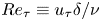 $Re_{\tau } \equiv u_{\tau } {\delta } / \nu$, where
 ${\delta }$ is the mean channel half-height, and
 $\nu$ is the kinematic viscosity. All simulations reported here were conducted at friction Reynolds number
 $395$. For cases with
 $ES_{y}>0.10$, a spanwise domain size
 $L_{2}/\delta =4.0$ was specified. For the three cases with
 $ES_{y}=0.10$, the spanwise domain size was increased by 50 % to
 $L_{2}/\delta =6.0$ to ensure that the topographical features decorrelate within the spanwise extent of the domain. Inner-scaled quantities are marked by superscript +, e.g. time
 $t^{+}=tu^{2}_{\tau }/\nu$, space
 $x_{i}^{+}=x_{i}u_{\tau }/\nu$, and velocity
 $u_{i}^{+}=u_{i}/u_{\tau }$. The key simulation parameters used throughout this study are consistent with the recommendations of Busse et al. (Reference Busse, Lützner and Sandham2015) and are listed in table 3.
For each simulation, data were accumulated for a minimum of  $Tu_{\tau }/\delta =40$ non-dimensional time units after the initial transient. In addition to collecting time-averaged data, instantaneous three-dimensional snapshots were also collected for further post-processing and analysis. Approximately 800 snapshots separated by twenty viscous-scaled time units, i.e.
 $\Delta t^{+}\equiv \Delta t u_{\tau }^{2}/\nu \approx 20$, were obtained for each case listed in table 3. Reference smooth-wall data were also accumulated at matched flow conditions for comparison.
2.3. Double-averaging methodology
Statistical quantities were computed using a time-then-space averaging procedure, more commonly known as double-averaging (Raupach & Shaw Reference Raupach and Shaw1982; Nikora et al. Reference Nikora, McEwan, McLean, Coleman, Pokrajac and Walters2007). An instantaneous field variable, say  $a(\boldsymbol {x},t)$, can be double-averaged (DA) by applying first the time-averaging operator,
 \begin{equation} \bar{a}(\boldsymbol{x})\equiv\lim_{T\rightarrow\infty}\frac{1}{T} \int_{t_{0}}^{t_{0}+T}{a}(\boldsymbol{x},t)\,\textrm{d}t, \end{equation}
and then the spatial-averaging operator,
 \begin{equation} \langle \bar{a}\rangle(x_{3}) \equiv \frac{1}{\phi(x_{3})}\,\frac{1}{A}\iint_{A}\bar{a} (\boldsymbol{x})\,\textrm{d}x_{1}\,\textrm{d}x_{2}. \end{equation}
In (2.3), the void fraction function 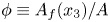 $\phi \equiv A_{f}(x_{3})/A$ represents the ratio of the fluid-occupied area to the total area of the wall-parallel plane,
 $A=L_{1}L_{2}$. Instantaneous field variables are set equal to zero in solid-occupied regions, i.e.
 $a(\boldsymbol {x},t)=0$. Averaging the flow in this way ensures that only fluid-occupied points contribute towards DA statistics beneath the roughness crests. The DA quantities reported herein therefore correspond to an intrinsic average (Gray & Lee Reference Gray and Lee1977).
Considering (2.2) and (2.3), instantaneous field variables are decomposed as
 \begin{equation} a(\boldsymbol{x},t) = {\underbrace{\langle \bar{a}\rangle(x_{3}) + \tilde{a}(\boldsymbol{x})}_{\bar{a}(\boldsymbol{x})}} + a^{\prime} (\boldsymbol{x},t), \end{equation}
where the dispersive component is defined as  $\tilde {a}(\boldsymbol {x})\equiv \bar {a}(\boldsymbol {x})-\langle \bar {a}\rangle (x_{3})$, and the turbulent component is defined as
 $a^{\prime }(\boldsymbol {x},t)\equiv a(\boldsymbol {x},t) - [\langle \bar {a}\rangle (x_{3}) + \tilde {a}(\boldsymbol {x})]$. Using the triple decomposition (2.4), the local Reynolds stress tensor can be defined as
 \begin{equation} \boldsymbol{\mathsf{R}}_{ij}(\boldsymbol{x})\equiv \overline{(u_{i}-\bar{u}_{i})(u_{j}-\bar{u}_{j})}= \overline{u^{\prime}_{i}u^{\prime}_{j}}. \end{equation}
The spatial average of the local Reynolds stress tensor 2.5 is defined here as
 \begin{equation} \langle \boldsymbol{\mathsf{R}}_{ij}\rangle(x_{3})\equiv \langle \overline{u^{\prime}_{i}u^{\prime}_{j}}\rangle. \end{equation}
Finally, the dispersive stress tensor is defined here as
 \begin{equation} \boldsymbol{\mathsf{D}}_{ij}(x_{3}) \equiv \left\langle {(\bar{u}_{i}-\langle \bar{u}_{i}\rangle)(\bar{u}_{j}-\langle \bar{u}_{j}\rangle)}\right\rangle=\langle \tilde{u}_{i}\tilde{u}_{j}\rangle. \end{equation}
3. Results
This section contains the key results of this study and is divided into four parts. First, the impact of  $ES_{y}$ upon the Hama roughness function is examined. Second, the effect of varying
 $ES_{y}$ upon the fractional contribution of pressure and viscous drag to the total drag is examined. Third, the influence of
 $ES_{y}$ upon first-order velocity statistics is discussed. Finally, the impact of
 $ES_{y}$ upon second-order velocity statistics and turbulence co-spectra is discussed.
3.1. Impact of spanwise effective slope upon the Hama roughness function
Surface roughness induces a downward shift in the log-law velocity profile, relative to the smooth-wall profile at matched flow conditions, commonly referred to as the Hama (Reference Hama1954) roughness function,  $\Delta U^{+}$. Strictly speaking,
 $\Delta U^{+}$ is an additive constant, which assumes that the inner-scale streamwise mean velocity difference between the smooth and rough walls – defined here as
 $\delta U^{+}(x^{+}_{3}) \equiv \langle u^{+}_{1}\rangle _{{s}}(x^{+}_{3})-\langle u^{+}_{1}\rangle _{{r}}(x^{+}_{3})$ – is uniform in the log region. Profiles of
 $\delta U^{+}$ normalised by the mean friction velocity are plotted against outer-scaled wall-normal position in figure 5. A histogram of the height distribution is also included (grey bars) and marks the wall-normal extent of the roughness canopy (
 $h_{\min }< x_{3}< h_{max}$). Looking from left-to-right across figures 5(a–c), it is clear that
 $\delta U^{+}$ remains approximately constant from the highest crest (
 $x_{3}/h_{max}=1$) to the channel half-height (
 $x_{3}/\delta =1$) for the majority of surfaces investigated here. Two exceptions are surface
 $022\_010$ (black dotted line in figure 5b) and surface
 $010\_010$ (red dotted line in figure 5a), with the latter surface showing an increase of almost 15 % when comparing the value of
 $\delta U^{+}$ at the channel half-height against that of the roughness crest. To remove any ambiguity related to variations of
 $\delta U^{+}$ in the outer region,
 $\Delta U^{+}$ is herein defined as the mean value of the streamwise velocity difference between the highest roughness crest and the channel half-height,
 $\Delta U^{+} \equiv 1/(\delta -h_{max})\int _{h_{max}}^{\delta }\delta U^{+}(x_{3})\,\textrm {d}x_{3}$. Other definitions of
 $\Delta U^{+}$ are possible: Chan et al. (Reference Chan, MacDonald, Chung, Hutchins and Ooi2015) defined
 $\Delta U^{+}$ as the streamwise velocity difference 50 wall units above the roughness crests in rough-wall turbulent pipe flow, whereas Busse et al. (Reference Busse, Lützner and Sandham2015) defined
 $\Delta U^{+}$ as the streamwise velocity difference at the centreline in rough-walled turbulent channel flow; Chung et al. (Reference Chung, Chan, MacDonald, Hutchins and Ooi2015) defined
 $\Delta U^{+}$ as the streamwise velocity difference at wall-normal height
 $z_{c}=0.4L_{3}$ in rough-wall minimal open-channel flow.
Streamwise velocity difference  $\delta U^{+}(x_{3})=\langle u_{1}^{+}\rangle _{s}-\langle u_{1}^{+}\rangle _{r}$ plotted as a function of wall-normal position for (a) Group A, (b) Group B, and (c) Group C. The histogram (grey) for each height distribution
 $P(h)$ is included for reference. All data are scaled using the mean friction velocity
 $u_{\tau }$ and mean channel half-height
 $\delta$.

The Hama roughness function is plotted as a function of  $ES_{y}$ in figure 6(a). Three key observations can be drawn from these data. First,
 $\Delta U^{+}$ varies by a factor of three (
 $2.5<\Delta U^{+}<7.6$) for the ten roughness topographies investigated here. Second,
 $\Delta U^{+}$ decreases monotonically as
 $ES_{y}$ increases for each value of
 $ES_{x}$. Third,
 $\Delta U^{+}$ becomes increasingly sensitive with respect to
 $ES_{y}$ as
 $ES_{x}$ is reduced. To be specific, whereas increasing
 $ES_{y}$ from 0.10 to 0.35 reduces
 $\Delta U^{+}$ by 12 % for surfaces with
 $ES_{x}\approx 0.35$ (blue symbols, Group C, figure 6a), a 35 % reduction is observed for surfaces with
 $ES_{x}\approx 0.10$ for the same change of
 $ES_{y}$ (red symbols, Group C, figure 6a). A further 23 % reduction in the Hama roughness function is observed for surface 010_070 (red diamond, figure 6a) relative to that of surface 010_035 (red circle, figure 6a), resulting in a
 $\Delta U^{+}$ value of just 2.4 wall units for the latter riblet-like surface. Together, these three observations demonstrate that
 $ES_{y}$ is an important topographical parameter, particularly for lower-
 $ES_{x}$ surfaces.
Hama roughness function  $\Delta U^{+}$ plotted as a function of (a) spanwise effective slope,
 $ES_{y}$, (b) streamwise effective slope
 $ES_{x}$, (c) ratio of spanwise and streamwise effective slopes
 $ES_{y}/ES_{x}$. Data points from the past work of Busse & Jelly (Reference Busse and Jelly2020) are also included (grey circles) for comparison, along with an an exponential fit (grey line) of the form
 $\Delta U^{+}=b_{1}+b_{2}\exp [-b_{3}(ES_{y}/ES_{x})^{2}]$, where
 $b_{i}=\{2.35,5.33,0.207\}$. Symbol types are given in table 3.

The Hama roughness function is plotted against  $ES_{x}$ in figure 6(b). In line with the findings of Napoli et al. (Reference Napoli, Armenio and De Marchis2008) and others, increasing
 $ES_{x}$ from 0.10 to 0.35 causes
 $\Delta U^{+}$ to increase for each value of
 $ES_{y}$ considered here. However, it is important to note that
 $\Delta U^{+}$ may show the opposite trend for higher-
 $ES_{x}$ surfaces that fall within the dense regime (MacDonald et al. Reference MacDonald, Chan, Chung, Hutchins and Ooi2016). The Hama roughness function is plotted against the effective slope ratio
 $ES_{y}/ES_{x}$ in figure 6(c), where data points from Busse & Jelly (Reference Busse and Jelly2020) have been included for comparison. Despite their differing
 $ES_{x}$ and
 $ES_{y}$ combinations, a reasonable collapse between the two datasets is observed, and most of the
 $\Delta U^{+}$ values exhibit a similar dependence upon
 $ES_{y}/ES_{x}$. To be specific, the relationship between
 $\Delta U^{+}$ and
 $ES_{y}/ES_{x}$ can be approximated as an exponential function of the form
 $\Delta U^{+}=b_{1}+b_{2}\exp [-b_{3}(ES_{y}/ES_{x})^{2}]$, where the coefficients
 $b_{i}=\{2.35,5.33,0.207\}$ were determined via nonlinear regression. A similar dependence between
 $\Delta U^{+}$ and the SAR parameter was reported by Busse & Jelly (Reference Busse and Jelly2020). Whilst figure 6(c) shows that
 $\Delta U^{+}$ varies significantly across the range
 $0.3\lesssim ES_{y}/ES_{x}<7.0$ for a fixed value of
 $k^{+}$, predicting the limiting behaviour of
 $\Delta U^{+}$ using the available data remains challenging. For instance, for the case where
 $ES_{y}/ES_{x}\rightarrow \infty$ with
 $ES_{x} = 0$ and very low
 $ES_{y}$,
 $\Delta U^{+}$ would likely tend to zero, since this
 $ES_{x}$–
 $ES_{y}$ combination corresponds to an almost smooth surface. On the other hand, for
 $ES_{y}/ES_{x}\rightarrow \infty$ with
 $ES_{x} = 0$ and high
 $ES_{y}$, it is possible that
 $\Delta U^{+}\neq 0$, since this
 $ES_{x}$–
 $ES_{y}$ combination corresponds to a riblet-like surface, which could either increase or decrease the levels of (viscous) drag; e.g. see Gatti et al. (Reference Gatti, von Deyn, Forooghi and Frohnapfel2020). Also, since the data in figure 6(c) correspond for a fixed viscous-scaled roughness height
 $k^{+}\approx 65.8$, questions regarding how the limiting behaviour of
 $\Delta U^{+}$ varies with roughness Reynolds number remain open.
Nevertheless, figure 6(c) demonstrates that the Hama roughness function is sensitive with respect to surface anisotropy and gives insight into how  $ES_{y}/ES_{x}$ affects
 $\Delta U^{+}$ at a fixed roughness Reynolds number
 $k^{+}\approx 65.8$ . Whilst
 $\Delta U^{+}$ values have been obtained for a variety of anisotropic roughness in past work by Thakkar et al. (Reference Thakkar, Busse and Sandham2016) and Jouybari et al. (Reference Jouybari, Yuan, Brereton and Murillo2021), these studies not only were performed at different
 $k^{+}$ values compared to the present study, but also did not eliminate the potential effects of other key topographical parameters upon the drag penalty, e.g. skewness, or vary
 $ES_{y}$ or
 $ES_{x}$ in a systematic manner (see figure 2). As a result, a meaningful comparison against these past studies and the data plotted in figure 6(c) cannot be made. On the other hand, a direct comparison can be drawn against the past data of Busse & Jelly (Reference Busse and Jelly2020) (filled grey circles, figure 6c), since that work was performed at the same
 $k^{+}$ value as the present study and focused on near-Gaussian roughness with comparable
 $ES_{x}$ and
 $ES_{y}$ combinations.
3.2. Impact of spanwise effective slope upon pressure and viscous drag
To associate physical mechanisms to changes in  $\Delta U^{+}$ (figure 6), the fractional contributions of pressure and viscous drag to the total drag can be quantified. After some manipulation, the mean viscous and pressure forces per unit area acting on the surface can be written as
 $$\begin{gather} \left\langle F_{\nu}\right\rangle=\iint_{S}-\mu\left[2\,\frac{\partial \bar{u}_{1}}{\partial x_{1}}\,\frac{{\partial h}}{\partial x_{1}}+ \left(\frac{\partial \bar{u}_{1}}{\partial x_{2}} + \frac{\partial \bar{u}_{2}}{\partial x_{1}}\right) \frac{{\partial h}}{\partial x_{2}}-\left(\frac{\partial \bar{u}_{1}}{\partial x_{3}} + \frac{\partial \bar{u}_{3}}{\partial x_{1}}\right)\right]\frac{1}{\left\|\boldsymbol{\nabla} h\right\|}\,{\rm d} S, \end{gather}$$
 $$\begin{gather}\left\langle F_{p}\right\rangle=\iint_{S}\left[(\bar{p}_{s}-\bar{p}_{0})\,\frac{{\partial h}}{\partial x_{1}}\right]\frac{1}{{\left\|\boldsymbol{\nabla} h\right\|}}\,{\rm d} S. \end{gather}$$
In (3.1) and (3.2),  $\bar {p}_{0}$ is an arbitrary gauge pressure, taken here as the mean surface pressure, i.e.
 $\bar {p}_{0} \equiv A^{-1}\iint \bar {p}_{s}(x_{1},x_{2})\,{\rm d} A$,
 $\|\boldsymbol {\nabla } h\|$ is the magnitude of the surface normal vector, and
 ${\rm d} S$ is the incremental surface area. Further details regarding (3.1) and (3.2) are provided in Appendix B.
Since the present simulations were carried out under constant pressure gradient forcing, the mean hydrodynamic force balance can be expressed as  $\langle F_{p}\rangle +\langle F_{\nu }\rangle =1$ (where
 $\varPi =-1$). Hence the summed effect of pressure and viscous drag remains constant, but the relative contributions of
 $\langle F_{p}\rangle$ and
 $\langle F_{\nu }\rangle$ to the total drag force,
 $\langle F_{tot}\rangle \equiv \langle F_{p}\rangle +\langle F_{\nu }\rangle =1$, are free to vary. In the limit of streamwise homogeneous roughness (
 $ES_{x}\rightarrow 0$), pressure drag is equal to zero, and the force balance for the current channel flow configuration reduces to
 $-\varPi =\iint _{S}-\mu [({\partial \bar {u}_{1}}/{\partial x_{2}}) ({{\partial h}}/{\partial x_{2}})-{\partial \bar {u}_{1}}/{\partial x_{3}}]({1}/{\|\boldsymbol {\nabla } h\|})\,{\rm d} S$, which shows that changes in spanwise gradient of the height map, and hence changes in
 $ES_{y}$, influence directly the levels of viscous drag. The same force balance governs the drag-increasing (or drag-reducing) properties of other streamwise homogeneous surfaces, e.g. flow-aligned riblets (Gatti et al. Reference Gatti, von Deyn, Forooghi and Frohnapfel2020). Conversely, in the limit of spanwise homogeneous roughness (
 $ES_{y}\rightarrow 0$), the force balance for the current channel flow configuration reduces to
 $-\varPi =\iint _{S}-\mu [2({\partial \bar {u}_{1}}/{\partial x_{1}})({{\partial h}}/{\partial x_{1}})-({\partial \bar {u}_{1}}/{\partial x_{3}} + {\partial \bar {u}_{3}}/{\partial x_{1}})]({1}/{{\|\boldsymbol {\nabla } h\|}})+[(\bar {p}_{s}-\bar {p}_{0})({{\partial h}}/{\partial x_{1}})]({1}/{{\|\boldsymbol {\nabla } h\|}})\,{\rm d} S$, and is therefore independent of
 $ES_{y}$ by definition. For the present surfaces, the relative importance of pressure and viscous drag sits somewhere between these two limits.
The fractional contribution of spatially averaged pressure drag to the total drag force,  $\langle F_{p}\rangle /\langle F_{tot}\rangle$, is plotted against
 $ES_{y}$ and
 $ES_{x}$ in figures 7(a,b), respectively. Overall, the pressure drag data show the same trends as the corresponding
 $\Delta U^{+}$ data plotted in figure 6. In summary,
 $\langle F_{p}\rangle /\langle F_{tot}\rangle$ decreases as
 $ES_{y}$ increases for each value of
 $ES_{x}$ investigated here, and exhibits a heightened sensitivity with respect to
 $ES_{y}$ as
 $ES_{x}$ becomes smaller. Likewise, when
 $\langle F_{p}\rangle /\langle F_{tot}\rangle$ is plotted against
 $ES_{y}/ES_{x}$ (figure 7c), the pressure drag contribution decreases as
 $ES_{y}/ES_{x}$ increases, meaning that streamwise-elongated forms of surface roughness (
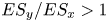 $ES_{y}/ES_{x}>1$) induce less pressure drag than their spanwise-aligned counterparts (
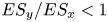 $ES_{y}/ES_{x}<1$). Note that the fractional contribution of spatially averaged viscous drag to the total drag force would show exactly the opposite trends, since
 $\langle F_{\nu }\rangle \equiv 1-\langle F_{p}\rangle$ for constant pressure gradient forcing.
Fractional contribution of spatially averaged pressure drag to the total drag force,  $\langle F_{p}\rangle /\langle F_{tot}\rangle$, plotted as a function of: (a) spanwise effective slope
 $ES_{y}$; (b) streamwise effective slope
 $ES_{x}$; (c) ratio of spanwise and streamwise effective slopes,
 $ES_{y}/ES_{x}$; and (d) the Hama roughness function
 $\Delta U^{+}$. Symbol types are given in table 3.

The fractional contribution of pressure drag is plotted as a function of  $\Delta U^{+}$ in figure 7(d). The data show that
 $\langle F_{p}\rangle /\langle F_{tot}\rangle$ varies by up to a factor of seven within the observed
 $\Delta U^{+}$ range. Specifically, pressure drag accounts for just 10 % (
 $\langle F_{p}\rangle /\langle F_{tot}\rangle \approx 0.1$) of the total drag on surface 010_070 (red diamond, figure 7d), compared to 74 % of the total drag (
 $\langle F_{p}\rangle /\langle F_{tot}\rangle \approx 0.74$) on surface 035_010 (blue square, figure 7d). Whilst the dependence of
 $\langle F_{p}\rangle /\langle F_{tot}\rangle$ on
 $ES_{x}$ is well-documented (Napoli et al. Reference Napoli, Armenio and De Marchis2008; MacDonald et al. Reference MacDonald, Chan, Chung, Hutchins and Ooi2016; Chan et al. Reference Chan, MacDonald, Chung, Hutchins and Ooi2018), the present data show that the fractional contribution of pressure drag ratio also depends on
 $ES_{y}$. However, a strong sensitivity with respect to
 $ES_{y}$ is expected only if the total wall drag has an appreciable viscous component. This is because the impact of spanwise variations in surface elevation, and hence variations in
 $ES_{y}$, upon hydrodynamic drag are transmitted through the viscous term (see (3.1)), which becomes increasingly small as the fully rough asymptote is approached. In other words, limited sensitivity with respect to
 $ES_{y}$ is to be expected when
 $\langle F_{p}\rangle \gg \langle F_{\nu }\rangle$.
Different criteria have been established in the literature to establish whether flow over a rough surface is in the fully rough regime. According to Scaggs, Taylor & Coleman (Reference Scaggs, Taylor and Coleman1988), the onset of the fully rough regime occurs when pressure drag accounts for more than 70 % of the total drag, i.e. 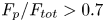 $F_{p}/F_{tot}>0.7$, meaning that only surface 035_010 in the present investigation should be considered fully rough (see figure 7). Jiménez (Reference Jiménez2004) defined the onset of the fully rough regime at
 $k_{s}^{+}>80$, which corresponds to a Hama roughness function
 $\Delta U_{FR}^{+}=\kappa ^{-1}\log (k_{s}^{+})-3.5\approx 7.5$ (assuming
 $\kappa =0.4$). Again, based on this criterion, only surface 035_010 should be considered fully rough (see figure 6) – nevertheless, its viscous drag is non-negligible at 25 %. Past work has also reported significant viscous effects in flows that exhibit fully rough behaviour. For instance, MacDonald, Hutchins & Chung (Reference MacDonald, Hutchins and Chung2019) reports that viscous drag still accounts for a quarter of the total drag in fully rough turbulent channel flow over three-dimensional egg-carton roughness at friction Reynolds number
 $Re_{\tau }=1680$, corresponding to an equivalent sand-grain roughness
 $k_{s}^{+}=300$. Likewise, Busse, Thakkar & Sandham (Reference Busse, Thakkar and Sandham2017) considered turbulent channel flow over irregular roughness up to friction Reynolds number
 $Re_{\tau }=720$. These authors reported that viscous effects account for approximately 33 % of the total drag at an equivalent sand-grain roughness
 $k_{s}^{+}\approx 150$. Nevertheless, the majority of the present data fall into the transitionally rough regime.
To better understand how varying  $ES_{y}$ affects the ratio
 $\langle F_{p}\rangle /\langle F_{tot}\rangle$ on Group A surfaces, the local values of time-averaged pressure drag can be examined. Contour plots of the time-averaged pressure drag on the four surfaces belonging to Group A surfaces are shown in figure 8. Whereas large patches of high-pressure drag (red contours) and low-pressure drag (blue contours) are evident on the windward and leeward faces of surfaces 010_010 and 010_022 (figures 8a,b), the pressure drag distribution on surfaces 010_035 and 010_070 (figures 8c,d) is comparably weak and sparse. A simple explanation for this behaviour is that the streamwise component of the surface normals on streamwise-elongated roughness tend to be small, and as a result, a weaker pressure drag force is exerted against the wall. The integrated effect of this behaviour explains why
 $\langle F_{p}\rangle /\langle F_{tot}\rangle$ decreases as
 $ES_{y}$ increases (figure 7b) and also why pressure drag decreases as
 $ES_{y}/ES_{x}$ increases (figure 7c). Iso-surfaces of time-averaged reverse flow are also included as transparent cyan blobs in figure 8. The volume of the time-averaged reverse flow regions decreases as
 $ES_{y}$ increases, which implies that flow separation downwind of roughness crests is suppressed for flow-aligned roughness, ultimately reducing the fractional contribution of spatially averaged pressure drag to the total drag (see figure 7d).
Time-averaged pressure drag force  $-(\bar {p}^{+}-\bar {p}^{+}_{0}){\partial h }/{\partial x_{1}}$ (the integrand of term
 $\langle F_{p}\rangle$ in (3.2)) for surfaces (a) 010_010, (b) 010_022, (c) 010_035, and (d) 010_070. Iso-surfaces of time-averaged reverse flow
 $(\bar {u}_{1}^{+}=-0.1)$ are shown as transparent cyan blobs. Data are shown on a
 $(3\times 3)/\delta$ sub-tile, where
 $\delta$ is the mean channel half-height.

The bulk flow properties for the rough- and smooth-wall cases are summarised in table 4. Since the friction Reynolds number is equal to 395 for all cases, the rise in the mean momentum deficit can be inferred from a reduction of the bulk Reynolds number  $Re_{b}$ or the centreline Reynolds number
 $Re_{cl}$, or an increase in the Hama roughness function
 $\Delta U^{+}$. Recalling that each surface considered here has a common mean peak-to-valley height and a near-Gaussian height distribution (table 2), the bulk properties listed in table 4, together with the variation of the Hama roughness function (figure 6) and the fractional contribution of spatially averaged pressure drag (figure 7), demonstrate that
 $ES_{y}$ is an important topographical parameter – particularly for low-
 $ES_{x}$ surfaces. Next, the impact of
 $ES_{y}$ upon first-order velocity statistics will be examined.
Bulk flow properties, including the friction Reynolds number  $Re_{\tau }$, centreline Reynolds number
 $Re_{cl}\equiv U_{cl}\delta /\nu$, bulk Reynolds number
 $Re_{b}\equiv U_{b}\delta /\nu$, viscous-scaled centreline velocity
 $(U^{+}_{cl})$, viscous-scaled bulk velocity
 $U^{+}_{b}$, ratio of centreline and bulk velocities
 $U_{cl}/U_{b}$; Hama roughness function
 $\Delta U^{+}$; skin-friction coefficient
 $C_{f}\equiv {2}/({U_{b}^{+2}})$; and fractional contribution of spatially averaged pressure drag to total drag,
 $\langle F_{p}\rangle /\langle F_{tot}\rangle$.

3.3. Impact of spanwise effective slope on first-order velocity statistics
Double-averaged (DA) streamwise velocity profiles normalised by the mean friction velocity are plotted against inner-scaled wall-normal position in figure 9, where reference smooth-wall data at matched flow conditions are included for comparison. Looking from left to right across figures 9(a–c), it is clear that most of the data exhibit a (nominal) log-law of the form
 \begin{equation} \left\langle \bar{u}^{+}_{1}\right\rangle = \kappa^{{-}1}\log \left(x_{3}^{+} + \epsilon\right)+ B - \Delta U^{+}, \end{equation}
where  $\kappa \approx 0.4$ is the von Kármán constant,
 $\epsilon$ is the virtual origin shift, and
 $B\approx 5.0$ is the smooth-wall intercept. Note that the virtual origin shift of the DA velocity profile was chosen to coincide with the mean roughness plane, i.e.
 $\epsilon \equiv \langle h\rangle =0$. This choice of
 $\epsilon$ is consistent with past studies of turbulent channel flow with irregular rough walls with comparable values of
 $ES_{x}$ and
 $ES_{y}$ (Thakkar et al. Reference Thakkar, Busse and Sandham2016; Peeters & Sandham Reference Peeters and Sandham2019; Portela et al. Reference Portela, Busse and Sandham2021), as well as studies of turbulent pipe flow over three-dimensional egg-carton roughness (Chan et al. Reference Chan, MacDonald, Chung, Hutchins and Ooi2015, Reference Chan, MacDonald, Chung, Hutchins and Ooi2018).
Effect of varying  $ES_{y}$ upon the DA inner-scaled streamwise velocity profile
 $\langle u_{1}\rangle ^{+}(x_{3})$ for surfaces in (a) Group A, (b) Group B, and (c) Group C. Line types are defined in table 3. The smooth-wall log-law
 $\kappa ^{-1}\log x_{3}^{+}+B$ is also included, where
 $\kappa =0.4$ and
 $B=5.0$.

In line with the values of  $\Delta U^{+}$ shown in figure 6, the downward shift of the log-law observed in figure 9 decreases as
 $ES_{y}$ increases for each value of
 $ES_{x}$ investigated here. However, whilst the velocity profiles exhibit a logarithmic dependence over the wall-normal range
 $50\lesssim x^{+}_{3}\lesssim 200$, the slope of the log region above some surfaces appears to differ from the smooth-wall data. In particular, the log region for surfaces 010_010 (red dotted line in figure 9a) and 022_010 (black dotted line in figure 9b) exhibit a shallower slope than the reference smooth-wall data (grey line), which is consistent with the non-uniform streamwise velocity difference observed previously in figure 5(a).
A further evaluation of the DA streamwise velocity profiles using the log-law diagnostic quantity  $\gamma =x_{3}^{+}\,\textrm {d}\langle \bar {u}_{1}\rangle /\textrm {d}x^{+}_{3}$ (George Reference George2007) is presented in figure 10. Whilst an extensive log region is not evident in the current data, the diagnostic function shows consistent behaviour with the outer region of the DA streamwise velocity profiles (see figure 9). To be specific, the log-law diagnostic function for Group C shows limited sensitivity with respect to
 $ES_{y}$, whereas Group A shows the opposite trend. In addition, whilst the log-law diagnostic function for Group C resembles the smooth-wall data in the outer region, appreciable differences emerge above Group A and B surfaces, which become more pronounced as
 $ES_{y}$ is reduced. Together, the change in the log-law slope above surfaces 010_010 (red dotted line in figure 9a) and 022_010 (black dotted line in figure 9b), and the deviations between the smooth- and rough-wall log-law diagnostic functions in the outer region (figure 10), hint at the presence of non-equilibrium effects and imply that the DA velocity profiles for these two particular surfaces may not recover mean flow outer-layer similarity.
Effect of varying  $ES_{y}$ upon the log-law diagnostic function
 $\gamma =x_{3}^{+}\,\textrm {d}\langle \bar {u}_{1}\rangle /\textrm {d}x^{+}_{3}$, for (a) Group A, (b) Group B, and (c) Group C surfaces. The histogram for each height distribution
 $P(h)$ is included for reference in grey. The horizontal black dashed line corresponds to
 $\gamma =1/\kappa$, where
 $\kappa$ was taken to be 0.4. Line types are defined in table 3.

To better illustrate the presence (or absence) of mean flow outer-layer similarity, the DA velocity profiles (figure 9) were recast into velocity-defect form,
 \begin{equation} \frac{\langle {u}^{}_{1}\rangle_{cl}-\langle {u}^{}_{1}\rangle}{u_{\tau}} = f\left(\dfrac{x_{3}}{\delta}\right), \end{equation}
where  $f$ is a universal function assumed independent of the viscous-scaled surface condition. While outer-layer similarity is typically investigated in the context of high-Reynolds-number flows and low
 $k/\delta$ using experimental methods (see e.g. Flack, Schultz & Shapiro Reference Flack, Schultz and Shapiro2005), many DNS studies at more moderate Reynolds numbers and comparatively high
 $k/\delta$ ratios have also observed a high degree of outer-layer similarity (Chan et al. Reference Chan, MacDonald, Chung, Hutchins and Ooi2015; Thakkar et al. Reference Thakkar, Busse and Sandham2016; Forooghi et al. Reference Forooghi, Stroh, Schlatter and Frohnapfel2018b; Jelly & Busse Reference Jelly and Busse2019b). However,
 $k/\delta$ and
 $Re_{\tau }$ are not the only length scale ratios that determine the degree of outer-layer similarity. Specifically, there is a growing body of literature showing that diminished levels of outer-layer similarity emerge when the in-plane spanwise roughness length scale approaches
 $\delta$ – including experimental investigations where low
 $k/\delta$ and high
 $Re_{\tau }$ could be achieved; e.g. see work by Nugroho, Hutchins & Monty (Reference Nugroho, Hutchins and Monty2013), Wangsawijaya et al. (Reference Wangsawijaya, Baidya, Chung, Marusic and Hutchins2020) and Nugroho et al. (Reference Nugroho, Monty, Utama, Ganapathisubramani and Hutchins2021). Such scenarios are possible for particular low-
 $ES_{y}$ surfaces considered in the present study, e.g. surface 010_010 whose in-plane spanwise roughness length scale is almost twice as large as the channel half-height, i.e.
 $\overline {\lambda _{y}}/\delta \approx 2$, as shown in figure 4).
DA velocity defect profiles are plotted against outer-scaled wall-normal position in figure 11, where reference smooth-wall data at matched flow conditions are included for comparison. Looking from left to right across figures 11(a–c), it is clear that Group C (blue lines, figure 11c) data show excellent levels of outer-layer similarity, and that varying  $ES_{y}$ has little to no effect on the flow in the outer region (see inset of figure 11(c) for a close-up view). Group C data are therefore in strong support of Townsend's outer-layer similarity hypothesis (Townsend Reference Townsend1976), which states that the roughness merely increases the surface stress, without causing structural changes in the outer region. In contrast, Group A data (red lines, figure 11a) show progressively poor levels of mean flow outer-layer similarity as
 $ES_{y}$ is reduced. In particular, the velocity-defect profile for surface 010_010 (red dotted line, figure 11a) begins to coincide with the smooth-wall data only above wall-normal heights greater than
 $x_{3}/\delta \gtrsim 0.8$ – implying that roughness effects penetrate deep into the outer layer, and mean flow distortion occurs on a scale commensurate with the channel half-height
 $\delta$. Diminished levels of mean flow outer-layer similarity have also been reported in recent studies above multi-scale cuboid elements (Medjnoun et al. Reference Medjnoun, Rodriguez-Lopez, Ferreira, Griffiths, Meyers and Ganapathisubramani2021) and above irregular roughness with
 $ES_{x}=ES_{y}\approx 0.08$ (Nugroho et al. Reference Nugroho, Monty, Utama, Ganapathisubramani and Hutchins2021). In both of these studies, reduced levels of outer-layer similarity were attributed to the emergence of large-scale roughness-induced motions on the cross-stream plane.
Effect of varying  $ES_{y}$ upon DA streamwise velocity defect profile
 $\langle u_{1,cl}\rangle ^{+}-\langle u_{1}\rangle ^{+}(x_{3})$ for (a) Group A, (b) Group B, and (c) Group C surfaces. The histogram for each height distribution
 $P(h)$ is included for reference in grey. Line types are defined in table 3.

Contours of streamwise dispersive velocity  $\tilde {u}^{}_{1}(\boldsymbol {x})\equiv \bar {u}_{1}(\boldsymbol {x})-\langle u_{1}\rangle (x_{3})$ are compared on the cross-stream plane for surfaces 010_010 and 010_070 in figures 12(a) and 12(b), respectively. Whereas the spanwise variation in the streamwise dispersive velocity is confined to wall-normal heights less than
 $x_{3}/\delta \lesssim 0.1$ above the latter surface, the former, lower-
 $ES_{y}$ surface shows a markedly different behaviour. In particular, the spanwise variation in streamwise dispersive stress above surface 010_010 extends up to (and beyond) the channel half-height (
 $x_{3}/\delta =1$), which implies that the portion of time-averaged flow with spatial inhomogeneity induced by the roughness elements (i.e. the roughness sublayer) fills the entire channel. Past work by Chan et al. (Reference Chan, MacDonald, Chung, Hutchins and Ooi2018) suggests that dispersive stresses (see (2.7)) extend up to height
 $x_{3}=0.5{\bar {\lambda }}_{y}$ in the wall-normal direction. This limit is shown as the horizontal dashed line in figure 12, and predicts approximately the wall-normal extent of streamwise dispersive velocity above both surfaces 010_010 and 010_070.
Effect of increasing  $ES_{y}$ upon cross-stream distribution of streamwise dispersive velocity
 $\tilde {u}^{}_{1}(\boldsymbol {x})\equiv \bar {u}_{1}(\boldsymbol {x})-\langle u_{1}\rangle (x_{3})$ for (a) surface 010_010 at
 $x_{1}/\delta =0.23$, and (b) surface 010_070 at
 $x_{1}/\delta =4.78$. The mean spanwise wavelength
 $\bar {\lambda }_{y}$ is represented by the width of the horizontal double-headed arrow. The horizontal dashed line shows the approximate wall-normal extent of the dispersive stresses
 $x_{3}=0.5\bar {\lambda }_{y}$ proposed by Chan et al. (Reference Chan, MacDonald, Chung, Hutchins and Ooi2018).

Considering the impact that reducing  $ES_{y}$ has upon the thickness of the roughness sublayer (figure 12), the diminished level of outer-layer similarity above surface 010_010 is arguably caused by inadequate scale separation between
 $\bar {\lambda }_{y}$ and
 $\delta$. More specifically, whilst the blockage ratio for surface 010_010 is
 $k/\delta =1/6$ (where
 $k$ is taken to be the mean peak-to-valley height
 $S_{z,{5\times 5}}$), which is the same
 $k/\delta$ value used in past studies where good levels of outer-layer similarity were observed (Thakkar et al. Reference Thakkar, Busse and Sandham2016; Jelly & Busse Reference Jelly and Busse2018; Portela et al. Reference Portela, Busse and Sandham2021), the ratio between
 $\bar {\lambda }_{y}$ and
 $\delta$ is approximately twelve times greater (
 $\bar {\lambda }_{y}/\delta \approx 2$, red square, upper right quadrant of figure 4). On the other hand, the ratio between
 $\bar {\lambda }_{y}$ and
 $\delta$ is an order of magnitude smaller for surface 010_070 (
 $\bar {\lambda }_{y}/\delta \approx 0.2$, red diamond, lower right quadrant of figure 4), which shows negligible spanwise variation in streamwise dispersive velocity in the outer region (figure 12b) and excellent levels of outer-layer similarity (red dash-dot line, figure 9a). Considering also that the in-plane streamwise mean wavelengths on surfaces 010_010 and 010_070 both exceed the outer length scale, i.e.
 $\bar {\lambda }_{x}/\delta >1$ (see figure 4), the diminished levels of outer-layer similarity above the former surface occur as a direct result of insufficient scale separation between
 $\bar {\lambda }_{y}$ and
 $\delta$, as opposed to between
 $\bar {\lambda }_{x}$ and
 $\delta$ or between
 $k$ and
 $\delta$. This is consistent with recent work by Nugroho et al. (Reference Nugroho, Monty, Utama, Ganapathisubramani and Hutchins2021), who noted that the wall-normal extent of roughness-induced flow patterns becomes large relative to
 $\delta$ where the in-plane roughness length scale approaches the local boundary-layer thickness, ultimately limiting the overall levels of outer-layer similarity. However, that work focused on an isotropic irregular roughness with
 $ES_{x}=ES_{y}\approx 0.08$ and the impact of varying
 $\bar {\lambda }_{y}$, and hence
 $ES_{y}$ could not be delineated from its streamwise counterpart.
To further characterise roughness-induced motions on the cross-plane (figure 12), secondary flow patterns were educed from the time-averaged velocity field  $\bar {u}_{i}(\boldsymbol {x})$ using a technique similar to that employed by Adrian, Christensen & Liu (Reference Adrian, Christensen and Liu2000) to identify instantaneous vortical structures on the streamwise-radial plane of turbulent pipe flow using planar particle image velocimetry data. The signed swirling strength, defined here as
 $\bar {\varLambda }_{ci}\equiv \lambda _{ci}(\bar {\omega }_{1}/|\bar {\omega }_{1}|)$, was computed by evaluating the imaginary component of the complex conjugate eigenvalue
 $\lambda _{ci}$ of the two-dimensional time-averaged velocity gradient tensor, which can written as
 \begin{equation}
\overline{\boldsymbol{\mathsf{d}}}_{ij,2D}\left(x_{2},x_{3}\right)=\left[\begin{array}{@{}cc@{}}
\dfrac{\partial \bar{u}_{2} }{\partial x_{2}} &
\dfrac{\partial \bar{u}_{2} }{\partial x_{3}} \\
\dfrac{\partial \bar{u}_{3} }{\partial x_{2}} &
\dfrac{\partial \bar{u}_{3} }{\partial x_{3}}
\end{array}\right] \end{equation}
on successive cross-stream planes. Note that  $(\bar {\omega }_{1}/|\bar {\omega }_{1}|)$ is the sign of the time-averaged streamwise vorticity
 $\bar {\omega }_{1}(\boldsymbol {x})=\partial \bar {u}_{2}/\partial x_{3}-\partial \bar {u}_{3}/\partial x_{2}$. Hence
 $\varLambda _{ci}\neq 0$ indicates the presence of local (steady) vortical motion, with
 $\varLambda _{ci}>0$ and
 $\varLambda _{ci}<0$ corresponding to clockwise and counter-clockwise rotation, respectively.
Iso-surfaces of time-averaged signed swirling strength  $\bar {\varLambda }_{ci}(\boldsymbol {x})$ for the four surfaces in Group A are shown in figure 13, where the value of
 $ES_{y}$ increases from top to bottom. Data are visualised above a
 $(4\times 4)/\delta$ sub-tile, where red iso-surfaces indicates clockwise rotation, and blue iso-surfaces indicates the opposite. Looking at figures 13(a–d), it is clear that the spatial characteristics of the time-averaged secondary flows are strongly affected by
 $ES_{y}$. For instance, the secondary flow patterns corresponding to surface 010_070 (figure 13a) strongly resemble the streamwise homogeneous counter-rotating vortex pairs that form above strip-type roughness (Yang & Anderson Reference Yang and Anderson2018) and are confined to wall-normal heights less than
 $x_{3}/\delta \lesssim 0.1$ in a manner similar to the cross-plane distribution of streamwise dispersive velocity (figure 12b). On the other hand, the secondary flow patterns above surface 010_010 (figure 13d) appear relatively incoherent in both the streamwise and spanwise directions, and extend far from the wall into the outer region of the flow, which, again, is consistent with the cross-plane distribution of streamwise dispersive velocity (figure 12a).
Effect of increasing  $ES_{y}$ upon iso-surfaces of the time-averaged signed swirl strength
 $\bar {\varLambda }_{ci}=0.005$ (red) and
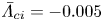 $\bar {\varLambda }_{ci}=-0.005$ (blue), for surfaces (a) 010_070, (b) 010_035, (c) 010_022, and (d) 010_010. Data are shown on a
 $(4\times 4)/\delta$ sub-tile, where
 $\delta$ is the mean channel half-height.

Overall, the observations drawn from figure 13 are consistent with recent studies regarding the formation of turbulent secondary flows over streamwise-aligned surfaces composed of spanwise alternating smooth and rough strips in channels (Yang & Anderson Reference Yang and Anderson2018), boundary layers (Wangsawijaya et al. Reference Wangsawijaya, Baidya, Chung, Marusic and Hutchins2020) and Taylor–Couette flows (Bakhuis et al. Reference Bakhuis, Ezeta, Berghout, Bullee, Tai, Chung, Verzicco, Lohse, Huisman and Sun2020). For this particular type of roughness, the (time-averaged) secondary flow behaviour is determined by the ratio of the spanwise wavelength  $\bar {\lambda }_{y}=2S$, where
 $S$ is the width of the strips, and the local boundary layer thickness
 $\delta$, and falls into one of three categories, e.g. see Chung, Monty & Hutchins (Reference Chung, Monty and Hutchins2018). (i) For
 $\bar {\lambda }_{y}/\delta \ll 0.5$ (or
 $S/\delta \ll 1$), the secondary flow is confined to the near-wall region and the flow is spanwise homogeneous above wall-normal heights greater than
 $x_{3}/\bar {\lambda }_{y}\approx 2$ (or
 $x_{3}/S\approx 1$), which is reminiscent of the cross-plane distribution of streamwise dispersive velocity above surface 010_070 (see figure 12b) and the corresponding iso-surfaces of signed swirling strength (see figure 13a). (ii) For
 $\bar {\lambda }_{y}/\delta \gg 2$ (or
 $S/\delta \gg 1$), the secondary flow is space-filling, characterised by
 $\delta$-scale motions separated by regions of spanwise homogeneous flow. (iii) For
 $\bar {\lambda }_{y}/\delta \approx 2$ (or
 $S/\delta \approx 1$), the secondary flow is also space-filling, but the
 $\delta$-scale motions occupy the entire cross-plane, which is reminiscent of the cross-plane distribution of streamwise dispersive velocity above surface 010_010 (see figure 12a) and the corresponding iso-surfaces of signed swirling strength (see figure 13d). Considering (i)–(iii), the present data suggest that the ratio
 $\bar {\lambda }_{y}/\delta$ plays an analogous role in determining secondary flow behaviour above the irregular three-dimensional roughness under investigation here.
3.4. Impact of spanwise effective slope on second-order velocity statistics
To further understand how  $ES_{y}$ affects the wall-normal extent of roughness-induced flow patterns, dispersive stresses were computed and examined. Dispersive stresses represent momentum flux in the near-roughness region due to spatial heterogeneity in the time-averaged flow, and arise as a direct result of time-then-space averaging (Pokrajac, McEwan & Nikora Reference Pokrajac, McEwan and Nikora2008) (see (2.7)). Profiles of the dispersive normal stresses normalised by the square of the mean friction velocity are plotted against outer-scaled wall-normal position in figure 14. Whist the dynamical significance of ‘form-induced’ stress in the near-wall region is well-documented (Moltchanov, Bohbot-Raviv & Shavit Reference Moltchanov, Bohbot-Raviv and Shavit2011; Ma et al. Reference Ma, Alamé and Mahesh2021), it is often assumed to vanish in the outer layer (Meyers, Ganapathisubramani & Cal Reference Meyers, Ganapathisubramani and Cal2019). Looking from left to right across figure 14, it is clear that whilst the magnitude of the spanwise dispersive stress
 $D_{22}$ is effectively zero in the outer region for all surfaces considered here (figures 14d–f), the remaining streamwise
 $D_{11}$ and wall-normal
 $D_{33}$ stresses do not necessarily follow the same trend. In particular, the latter component shows persistent levels well into the outer region for surface 010_010 (red dotted line in figure 14a), surface 010_022 (red dashed line in figure 14a), and, to a slightly lesser extent, surface 022_010 (black dotted line in figure 14b). These are the same three low-
 $ES_{y}$ surfaces that exhibit a non-uniform streamwise velocity difference in the outer region (figure 5), non-universal coefficients in their respective log laws (figure 9), and diminished levels of outer-layer similarity (figure 11), which again underlines the growing significance of
 $ES_{y}$ as
 $ES_{x}$ becomes smaller. In addition, the wall-normal persistence of dispersive stresses observed in figure 14 challenges the classical picture of an outer layer that is dominated by Reynolds stresses (Castro Reference Castro2007) and therefore motivates an analysis of second-order turbulence statistics.
Effect of varying  $ES_{y}$ upon dispersive normal stresses
 $\boldsymbol{\mathsf{D}}_{ii}(x_{3})$. Streamwise dispersive stresses
 $D_{11}(x_{3})$ for (a) Group A, (b) Group B, and (c) Group C surfaces. Spanwise dispersive stresses
 $D_{22}(x_{3})$ for (d) Group A, (e) Group B, and ( f) Group C surfaces. Wall-normal dispersive stresses
 $D_{33}(x_{3})$ for (g) Group A, (h) Group B, and (i) Group C surfaces. The histogram for each height distribution
 $P(h)$ is included for reference in grey. Line types are defined in table 3.

Profiles of spatially averaged streamwise Reynolds stress  $\langle R_{11}\rangle$ normalised by the square of the mean friction velocity are plotted against outer-scaled wall-normal position for Groups A, B and C in figure 15. Looking from left to right across figures 15(a–c), it is clear that the best collapse between the smooth- and rough-wall data is observed for Group C (blue lines). These data are therefore in strong support of Townsend's outer-layer similarity hypothesis (Townsend Reference Townsend1976), which states that the turbulent stresses, normalised by the square of the mean friction velocity, are universal outside the roughness sublayer, which can be written as
 \begin{equation} \frac{\langle \boldsymbol{\mathsf{R}}_{ij}\rangle}{u_{\tau}^{2}} = g_{ij}\left(\frac{x_{3}}{\delta}\right), \end{equation}
where  $g_{ij}$ is a universal function hypothesised to be independent of the viscous-scaled surface condition. On the other hand, the streamwise Reynolds stress profile above surface 010_010 (dotted red line, figure 15a) and surface 010_022 (dotted black line, figure 15b) shows the worst overall collapse with the smooth-wall data, which is consistent with the behaviour of the log-law diagnostic functions (see figure 10) and velocity defect profiles (see figure 11). As was mentioned previously, one explanation for this behaviour is that as
 $\bar {\lambda }_{y}$ approaches
 $\delta$, the roughness sublayer thickens, ultimately perturbing streamwise velocity fluctuations from their ‘equilibrium’ state. Past work has also reported diminished levels of outer-layer similarity on Reynolds stresses above roughness with long wavelength features in the spanwise direction – the limiting case being two-dimensional spanwise bars with
 $\bar {\lambda }_{y}/\delta \rightarrow \infty$. For instance, Volino, Schultz & Flack (Reference Volino, Schultz and Flack2011) reported a breakdown of outer-layer similarity for Reynolds stresses in turbulent boundary-layer flow over two-dimensional bar roughness, but not for three-dimensional cube roughness, despite the latter being a factor three times larger than the smallest bars in terms of
 $k$. Although the roughnesses considered by Volino et al. (Reference Volino, Schultz and Flack2011) have a fundamentally different character compared to the irregular, three-dimensional roughness under consideration in the present study – e.g. the former have fixed separation points whereas the latter does not – there is qualitative similarity in the sense that when
 $ES_{y}$ becomes low (and spanwise features become large), the roughness sublayers thicken, which, ultimately, may lead to a breakdown of outer-layer similarity.
Effect of varying  $ES_{y}$ upon spatially averaged streamwise Reynolds stresses
 $\langle R_{11}\rangle (x_{3})$ for (a) Group A, (b) Group B, and (c) Group C surfaces. Effect of varying
 $ES_{y}$ upon the sum of spatially averaged streamwise Reynolds stress and streamwise dispersive stress,
 $\langle R_{11}\rangle (x_{3})+D_{11}(x_{3})$, for (d) Group A, (e) Group B, and ( f) Group C surfaces. The histogram for each height distribution
 $P(h)$ is included for reference in grey. Line types are defined in table 3.

Profiles of the sum of the spatially averaged Reynolds stress and streamwise dispersive stress,  $\langle R_{11}\rangle +D_{11}$, for Groups A, B and C are shown in figures 15(d–f). Comparing these data against their Reynolds stress counterparts in (a–c), it is clear that observed levels of outer-layer similarity above Group C surfaces remain unaffected by the addition of streamwise dispersive stress, since
 $D_{11}$ decays to a negligible value in the outer region (see figure 14c). This observation is consistent with the results of Forooghi et al. (Reference Forooghi, Stroh, Schlatter and Frohnapfel2018b) and Busse & Jelly (Reference Busse and Jelly2020), which show that
 $D_{11}$ becomes negligible relative to
 $\langle R_{11}\rangle$ in the outer layer. In contrast, since
 $D_{11}$ remains non-negligible above surface 010_010 (red dotted line, figure 14a) and surface 022_010 (black dotted line, figure 14b) well into the outer layer, the profiles of
 $\langle R_{11}\rangle +D_{11}$ shift upwards, relative to the Reynolds stress profiles plotted in figure 15(a), and fail to collapse on the smooth-wall data at all wall-normal positions (red dotted line, figure 14d).
Profiles of spatially averaged Reynolds shear stress  $\langle R_{13}\rangle$, normalised by the square of the mean friction velocity, are plotted against wall-normal position for Groups A, B and C in figure 16, where smooth-wall data at matched flow conditions are included for comparison. Again, looking from left-to-right across figures 16(a–c), it is clear that the best collapse between the smooth- and rough-wall data is observed for Group C (blue lines), and the worst overall collapse is observed above surface 010_010 (dotted red line, figure 16a), which is in line with the behaviour of the corresponding streamwise Reynolds stress profile (red dotted line, figure 15a). One explanation for this behaviour is that the contribution of dispersive shear stress
 $\langle D_{13}\rangle$ to the total shear stress becomes increasingly large as
 $ES_{y}$ decreases. Assuming that the viscous shear stress is negligible for heights greater than
 $x_{3}/h_{max}>1$, the total shear stress varies linearly as
 $1-x_{3}/\delta \approx -(\langle R_{13}\rangle + \langle D_{13}\rangle )$ above the roughness crests, which means that any increase in dispersive shear stress must be met by a decrease in Reynolds shear stress (and vice versa). The sum of Reynolds and dispersive shear stress,
 $(\langle R_{13}\rangle +\langle D_{13}\rangle )$, normalised by the square of the mean friction velocity, is plotted against outer-scaled wall-normal position in figures 16(d–f). The data exhibit an almost perfect linear variation between the highest roughness crest (
 $x_{3}/h_{max}=1$) and the channel half-height (
 $x_{3}/\delta =1$), which, in addition to verifying that viscous stresses are indeed negligible in the outer region, also confirms that the present simulations have achieved satisfactory levels of statistical convergence; e.g. see Vinuesa et al. (Reference Vinuesa, Prus, Schlatter and Nagib2016) for details. Differences between the total shear stress (figures 16d–f) and spatially averaged Reynolds shear stress profiles (figures 16a–c) above the roughness crests therefore arise as a direct result of non-negligible dispersive shear stress, which increases above low-
 $ES_{x}$ surfaces as
 $ES_{y}$ is reduced.
Effect of varying  $ES_{y}$ upon spatially averaged Reynolds shear stress
 $\langle R_{13}\rangle (x_{3})$ for (a) Group A, (b) Group B, and (c) Group C surfaces. Effect of varying
 $ES_{y}$ upon the sum of spatially averaged Reynolds shear stress and dispersive shear stress,
 $\langle R_{13}\rangle (x_{3})+D_{13}(x_{3})$, for (d) Group A, (e) Group B, and ( f) Group C surfaces. The histogram for each height distribution
 $P(h)$ is included for reference in grey. Line types are defined in table 3.

To associate particular length scales to the levels of spatially averaged Reynolds shear stress (figure 16), the co-spectra of instantaneous  $u_{1}^{\prime }u_{3}^{\prime }$ fluctuations can be examined. This allows analysis of the energetic contributions from different wavelengths, e.g. in the streamwise direction,
 $\langle R_{13}\rangle ^{}(x_{3})=\int _{0}^{\infty }\varPhi ^{}_{13} (\lambda _{1},x_{3})\,\textrm {d}\log (\lambda _{1}^{})$, where
 $\varPhi ^{}_{13}(\lambda _{1},x_{3})=\kappa _{1}\,\phi ^{}_{13}(\lambda _{1},x_{3})$ is the premultiplied co-spectrum of
 $u_{1}^{\prime }$ and
 $u_{3}^{\prime }$, and
 $\kappa _{1}$ is the streamwise wavenumber. Whilst the behaviour and scaling of Reynolds shear stress co-spectra in smooth-walled turbulent channel flow are well-documented (Del Alamo et al. Reference Del Alamo, Jiménez, Zandonade and Moser2004; Lee & Moser Reference Lee and Moser2015), data are less common above irregular rough walls. Here, the spectral decomposition of Reynolds shear stress is compared for surfaces 010_010 and 010_035, and the reference smooth-wall data, with the aim of identifying the range of scales that exhibit the most (or least) sensitivity with respect to
 $ES_{y}$.
Contours of streamwise premultiplied Reynolds shear stress co-spectra normalised by the square of the mean friction velocity are plotted against inner-scaled wall-normal position for surfaces 010_035 and 010_010 in figures 17(a,b), respectively. Looking first at figure 17(a), it is clear that the co-spectra for surface 010_035 (blue lines) collapse on top of the smooth-wall data (grey lines) above wall-normal heights greater than  $x^{+}_{3}\gtrsim 100$. In addition, the peak energy in the streamwise premultiplied co-spectra occurs just above the roughness crests and is concentrated at wavelengths approximately equal to the mean streamwise roughness wavelength (
 $\bar {\lambda }_{x}/\delta \approx 1$, horizontal black line, figure 17a). Previous analyses of streamwise premultiplied energy spectra of streamwise velocity fluctuations in turbulent pipe flow above isotropic egg-carton roughness have shown similar behaviour at comparable flow conditions (Chan et al. Reference Chan, MacDonald, Chung, Hutchins and Ooi2018). Whilst the peak energy in the surface 010_010 co-spectra (red lines, figure 17b) also occurs just above the roughness crests and is concentrated at wavelengths approximately equal to the mean streamwise roughness wavelength, the data show a clear disagreement with the smooth-wall data above wall-normal heights greater than
 $x^{+}_{3}\gtrsim 100$ and for streamwise wavelengths greater than
 ${\lambda }^{+}_{x}\gtrsim 500$. This observation implies that the turbulence structure above surface 010_010 has undergone a broadband spectral change. To quantify these changes, the smooth-wall Reynolds shear stress co-spectrum was subtracted from its rough-wall counterpart using the formula
 $\Delta \varPhi ^{}_{13}(\lambda _{1},x_{3})\equiv \kappa _{1}[\phi ^{}_{13,r} (\lambda _{1},x_{3})-\phi ^{}_{13,s}(\lambda _{1},x_{3})]$, where subscripts
 $r$ and
 $s$ denote rough- and smooth-wall data, respectively.
Comparison of streamwise premultiplied Reynolds shear stress co-spectra between the reference smooth wall (grey line) and (a) surface 010_035 (blue line), and (b) surface 010_010 (red line). The vertical black lines on the lower and upper horizontal axis denote the height of the highest roughness crest ( $x_{3}/h_{max}=1$) and the wall-normal extent of the dispersive stresses
 $x_{3}=0.5\bar {\lambda }_{y}$ proposed by Chan et al. (Reference Chan, MacDonald, Chung, Hutchins and Ooi2018), respectively. The horizontal black line denotes the mean streamwise roughness wavelength (
 $\bar {\lambda }_{x}/\delta =1$). Vertical and horizontal black dashed lines denote the wall-normal height of the channel half-height (
 $x_{3}/\delta =1$) and the streamwise length of the computational domain (
 $L_{1}/\delta$), respectively. Contour lines in (a,b) are shown on the levels
 $\{0.05, 0.13, 0.21, 0.29\}$. The differences between the smooth-wall co-spectra and rough-wall co-spectra for (c) surface 010_035 and (d) surface 010_010 are also shown, where dotted and solid lines denote an energetic deficit (
 $\Delta \phi _{13}<0$) and surplus (
 $\Delta \phi _{13}>0$), respectively. Positive and negative contour lines in (c,d) are shown on the levels
 $\{0.025,0.043,0.062,0.080\}$ and
 $-\{0.025,0.050,0.075,0.100\}$, respectively.

The difference between the smooth-wall and surface 010_035 Reynolds shear stress co-spectra is shown in figure 17(c), where solid and dotted lines denote an energy surplus ( $\Delta \phi _{13}>0$) and an energy defect (
 $\Delta \phi _{13}<0$), respectively. As expected, negligible energetic differences (
 $\Delta \phi _{13}\approx 0$) are observed across all streamwise wavelengths above wall-normal heights greater than
 $x_{3}^{+}\gtrsim 100$, since the smooth- and rough-wall co-spectra collapse in the same region (see figure 17a). Negligible energetic differences are also observed where the roughness-induced secondary motions become small, i.e. above wall-normal heights greater than
 $x_{3}/\bar {\lambda }_{y}>0.5$, as proposed by Chan et al. (Reference Chan, MacDonald, Chung, Hutchins and Ooi2018) (see figure 12b). In contrast, an energy defect is evident in the vicinity of the highest roughness crests (
 $x_{3}/h_{max}=1$) for streamwise wavelengths greater than
 $\lambda _{x}^{+}\gtrsim 250$, with the strongest defect concentrated at wavelengths approximately equal to the mean streamwise roughness wavelength
 $(\bar {\lambda }_{x}/\delta \approx 1)$. The net effect of these energy-deficient scales explains why the peak value of the spatially averaged Reynolds shear stress profile is suppressed above surface 010_035 (dotted blue line, figure 16c), relative to the smooth-wall value (grey line, figure 16c), and is consistent with the notion that surface roughness disrupts the near-wall turbulence cycle (Schultz & Flack Reference Schultz and Flack2007; Squire et al. Reference Squire, Morrill-Winter, Hutchins, Schultz, Klewicki and Marusic2016). In the vicinity of the mean roughness height, an energy surplus is evident for streamwise wavelengths greater than
 $\lambda _{x}^{+}\gtrsim 180$, which explains why the levels of spatially averaged Reynolds shear stress around
 $x_{3}^{+}\approx 0$ for surface 010_035 (dotted blue line, figure 16c) exceed smooth-wall levels (grey line, figure 16c).
The difference between the smooth-wall and surface 010_010 co-spectra is shown in figure 17(d). In contrast to the surface 010_035 data (figure 17c), the data above surface 010_010 reveal an energy defect that penetrates deep into the outer region for streamwise wavelengths of the order of the mean streamwise roughness wavelength, i.e.  $\bar {\lambda }_{x}/\delta \approx 1.0$ (red dotted lines). The net effect of these energy-deficient scales explains why the Reynolds shear stress profile for surface 010_010 fails to collapse onto the smooth-wall data in the outer region (dotted red line, figure 16a) and why such poor levels of outer-layer similarity are observed. Further, the wall-normal extent of the energy defect above surface 010_010 is consistent with the height of the roughness sublayer inferred from the cross-stream distribution of streamwise dispersive velocity (figure 12a), as well as the dimensions of roughness-induced secondary motions identified using signed swirl strength (figure 13d).
Contours of spanwise premultiplied Reynolds shear stress co-spectra normalised by the square of the mean friction velocity are plotted against inner-scaled wall-normal position for surfaces 010_035 and 010_010 in figures 18(a,b), respectively. Overall, the spanwise co-spectra show similar trends to their streamwise counterparts (figures 17a,b). In particular, the spanwise co-spectra above surface 010_035 (figure 17c) show good levels of agreement with the smooth-wall data in the outer region, whereas the surface 010_010 data show obvious disagreement over a range of scales (figure 17d). The differences between the smooth-wall spanwise co-spectra and the data for surfaces 010_035 and 010_010 are shown in figures 18(c) and 18(d), respectively. Again, whilst negligible energetic differences are observed for wall normal heights greater than  $x_{3}^{+}\gtrsim 100$ above surface 010_035 (figure 18c), an energy defect extends deep into the outer region above surface 010_010 (figure 18d), which indicates that the turbulence structure, even far from the wall, is profoundly altered above the latter, lower-
 $ES_{y}$ surface. As a result, whereas diminished levels of outer-layer similarity are observed above surface 010_010, the surface 010_035 co-spectra retain outer-layer similarity on a scale-by-scale basis.
Comparison of spanwise premultiplied Reynolds shear stress co-spectra between the reference smooth wall (grey line) and (a) surface 010_035 (blue line), and (b) surface 010_010 (red, line). The vertical black lines on the lower and upper horizontal axis denote the height of the highest roughness crest ( $x_{3}/h_{max}=1$) and the wall-normal extent of the dispersive stresses
 $x_{3}=0.5\bar {\lambda }_{y}$ proposed by Chan et al. (Reference Chan, MacDonald, Chung, Hutchins and Ooi2018), respectively. The horizontal black line denotes the mean streamwise roughness wavelength (
 $\bar {\lambda }_{x}/\delta =1$). Vertical and horizontal black dashed lines denote the wall-normal height of the channel half-height (
 $x_{3}/\delta =1$) and the spanwise width of the computational domain (
 $L_{2}/\delta$), respectively. Contour lines in (a,b) are shown on the levels
 $\{0.05, 0.20, 0.35, 0.50\}$. The differences between the smooth-wall co-spectra and rough-wall co-spectra for (c) surface 010_035 and (d) surface 010_010 are also shown, where dotted and solid lines denote an energetic deficit (
 $\Delta \phi _{13}<0$) and surplus (
 $\Delta \phi _{13}>0$), respectively. Positive and negative contour lines in (c,d) are shown on the levels
 $\{0.050,0.075,0.100,0.125\}$ and
 $-\{0.050,0.083,0.117,0.150\}$, respectively.

4. Conclusions
Fully developed turbulent channel flow over irregular, three-dimensional rough walls with systematically varied values of spanwise effective slope ( $ES_{y}$) was studied using direct numerical simulations (DNS) at friction Reynolds number 395, corresponding to viscous-scaled roughness height
 $k^{+}\approx 65.8$ (where
 $k$ is the mean peak-to-valley height). A set of ten near-Gaussian roughness topographies with specified values of
 $ES_{y}$, three separate values of streamwise effective slope
 $ES_{x}$, and common mean peak-to-valley height, were synthesised using a surface generation algorithm (figure 3). The instantaneous DNS data were reduced using the double-averaged (DA) methodology, and the sensitivity of DA statistics with respect to
 $ES_{y}$ for each value of
 $ES_{x}$ was studied for a fixed value of
 $k^{+}$ in the context of the Hama roughness function (figures 5 and 6), the fractional contribution of spatially averaged pressure drag to total drag (figures 7 and 8), mean velocity profiles (figures 9 and 11), dispersive streamwise velocity (figure 12), roughness-induced secondary motions (figure 13), dispersive normal stresses (figure 14), spatially averaged Reynolds shear stress (figure 16) and Reynolds shear stress co-spectra (figures 17 and 18). The contributions of this work are discussed below.
The key finding of this work is that  $ES_{y}$ emerges as a key topographical parameter as its streamwise counterpart
 $ES_{x}$ becomes small. One interpretation of this behaviour is that
 $ES_{y}$ becomes more important as the ‘waviness’ regime is approached, which, according to Schultz & Flack (Reference Schultz and Flack2009), occurs for surfaces with
 $ES_{x}\lesssim 0.35$. In this regime, viscous drag can become non-negligible and the flow is considered to be transitionally rough. For instance, Napoli et al. (Reference Napoli, Armenio and De Marchis2008) report that viscous and pressure drag are approximately equal on two-dimensional irregular sine wave roughness with
 $ES_{x}=0.15$ at viscous-scaled mean absolute roughness height
 $k^{+}\approx 14$. MacDonald et al. (Reference MacDonald, Chan, Chung, Hutchins and Ooi2016) report that viscous drag dominates pressure drag on isotropic three-dimensional egg-carton roughness with
 $ES_{x}\lesssim 0.35$ at viscous-scaled sinusoidal semi-amplitude
 $k^{+}=10$. Under these conditions, spanwise variations in surface elevation,
 $\partial h/\partial x_{2}$, and hence variations in
 $S_{y}$, can affect directly the global force balance through the viscous term (3.1). However, it is worth noting that low-
 $ES_{x}$ surfaces that fall within the wavy regime can also exhibit fully rough behaviour, where viscous drag is overwhelmed by pressure drag
 $(F_{p}\gg F_{\nu })$. For instance, Nugroho et al. (Reference Nugroho, Monty, Utama, Ganapathisubramani and Hutchins2021) report fully rough behaviour for their ‘rough 2.5
 $\times$’ orange-peel surface (
 $ES_{x}=ES_{x}\approx 0.08$), where the Hama roughness function varies as
 $\Delta U_{FR}^{+}(k_{s}^{+})=\kappa ^{-1}\log C k^{+} +A-8.5$ (where
 $C=k_{s}/k\approx 2.45$, and
 $k$ is the mean absolute height). Under these flow conditions, it is possible that the Hama roughness function will exhibit limited sensitivity with respect to variations in
 $ES_{y}$, since its effect can no longer be transmitted through the viscous term. However, the effect of varying
 $ES_{y}$ under fully rough conditions was not investigated by Nugroho et al. (Reference Nugroho, Monty, Utama, Ganapathisubramani and Hutchins2021) since their work considered isotropic roughness (
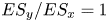 $ES_{y}/ES_{x}=1$). Most of the data in the present study fall within the transitionally rough regime, and as a result, an appreciable sensitivity with respect to
 $ES_{y}$ was retained – particularly for low-
 $ES_{x}$ surfaces that have the highest proportion of viscous drag. Past work by Thakkar et al. (Reference Thakkar, Busse and Sandham2016) and Jouybari et al. (Reference Jouybari, Yuan, Brereton and Murillo2021) has also identified
 $ES_{y}$ as an important topographical parameter at comparable flow conditions. The present study complements this past work by providing a detailed account of the physical mechanisms that determine the sensitivity of
 $\Delta U^{+}$ with respect to systematic variations in
 $ES_{y}$ for a fixed value of
 $k^{+}$.
A secondary finding of this work is that particular low- $ES_{y}$ surfaces investigated here can cause a breakdown of outer-layer similarity in both mean flow and turbulence statistics (for a fixed value of
 $k^{+}$). Diminished levels of outer-layer similarity became most pronounced for the lowest value of
 $ES_{x}$ and
 $ES_{y}$ investigated here (
 $ES_{x}=ES_{y}=0.1$). This behaviour was attributed to insufficient scale separation between the outer length scale
 $\delta$ and the in-plane spanwise roughness wavelength
 $\bar {\lambda }_{y}$. To be specific, as
 $\bar {\lambda }_{y}$ approaches
 $\delta$, spanwise variations in time-averaged streamwise velocity were observed to extend up to (and beyond) the channel half-height
 $\delta$. Similar observations have been made in the context of two-dimensional strip roughness (Yang & Anderson Reference Yang and Anderson2018), multi-scale cuboid roughness (Medjnoun et al. Reference Medjnoun, Rodriguez-Lopez, Ferreira, Griffiths, Meyers and Ganapathisubramani2021) and three-dimensional egg-carton roughness (Chan et al. Reference Chan, MacDonald, Chung, Hutchins and Ooi2018) when
 $\bar {\lambda }_{y}$ becomes an appreciable proportion of the boundary layer thickness. Here, the mean-squared effect of these
 $\delta$-scale motions led to non-negligible levels of dispersive stress in the outer region, which, as noted by Jelly & Busse (Reference Jelly and Busse2018), play a direct role in determining the the local value of
 $\Delta U^{+}$ above the roughness crests. An examination of Reynolds shear stress co-spectra also revealed diminished levels of outer-layer similarity above low-
 $ES_{y}$ surfaces, implying that the turbulence structure, even far from the wall, is affected across a wide range of energy-containing scales. Overall, these observations add to the growing body of literature that the thickness of the roughness sublayer is a direct function of the spanwise in-plane roughness wavelength (Chan et al. Reference Chan, MacDonald, Chung, Hutchins and Ooi2018; Medjnoun et al. Reference Medjnoun, Rodriguez-Lopez, Ferreira, Griffiths, Meyers and Ganapathisubramani2021) and that as this length scale becomes an appreciable fraction of the outer length scale, non-equilibrium behaviours emerge in both mean and turbulence statistics.
Supplementary material
Supplementary material is available at https://doi.org/10.1017/jfm.2022.823.
Funding
We gratefully acknowledge support by the United Kingdom Engineering and Physical Sciences Research Council via grant no. EP/P009875/1, and by the Australian Research Council. This work used the Cirrus UK National Tier-2 HPC Service at EPCC (http://www.cirrus.ac.uk) funded by the University of Edinburgh and EPSRC (EP/P020267/1). T.O.J. gratefully acknowledges the financial support of the University of Melbourne Early Career Researcher Award. A.B. gratefully acknowledges support via a Leverhulme Trust Research Fellowship.
Declaration of interests
The authors report no conflict of interest.
Data availability statement
Surface and velocity data are openly available from the University of Leicester research repository under https://doi.org/10.25392/leicester.data.21324765.
Appendix A. Numerical details of the surface synthesis procedure
Irregular surface roughness with specified statistical properties was generated using the multi-scale anisotropic rough surface (MARS) algorithm (Jelly & Busse Reference Jelly and Busse2018, Reference Jelly and Busse2019a). Doubly periodic height maps  $h_{ij}$ were synthesised by taking linear combinations of Gaussian random number matrices using a weighted moving average (MA) process, which can be expressed as
 \begin{equation}
h_{ij}=\sum_{k=1}^{n_{1}}\sum_{l=1}^{n_{2}}\alpha_{kl}\,\eta_{rs},\quad
\left\{\begin{array}{@{}l} i=1,2,\ldots,N_{1}, \\
j=1,2,\ldots,N_{2}, \\ r=\left[i+k-1\
\left(\bmod~N_{1}\right)\right]+1,\\ s=\left[j+l-1\
\left(\bmod~N_{2}\right)\right]+1, \end{array}\right.
\end{equation}
where  $\eta _{ij}$ is an
 $N_{1} \times N_{2}$ matrix of uncorrelated Gaussian random numbers, the
 $\alpha _{kl}$ are an
 $n_{1} \times n_{2}$ set of coefficients, and
 $\bmod$ denotes the modulo operator.
In (A1), the MA coefficients  $\alpha _{kl}$ were determined by solving the system of nonlinear equations
 \begin{equation}
R_{pq}=\sum_{k=1}^{n_{1}-p}\sum_{l=1}^{n_{2}-q}\alpha_{kl}\,\alpha_{k+p,l+q},\quad
\left\{\begin{array}{@{}l} p=0,1,\ldots,n_{1}-1, \\
q=0,1,\ldots,n_{2}-1, \end{array}\right.
\end{equation}
using an iterative Newton-based method outlined in past work by Patir (Reference Patir1978), where  $R_{pq}$ is the discrete autocorrelation function (ACF).
Each height map was generated with a specified exponential ACF
 \begin{equation} R(\Delta{x}_{1},\Delta{x}_{2})= \exp\left({-}2.3\sqrt{\left(\frac{\Delta{x}_{1}}{\Delta{x}^{*}_{1}}\right)^{2} + \left(\frac{\Delta{x}_{2}}{\Delta{x}^{*}_{2}}\right)^{2}}\right), \end{equation}
where  $\Delta {x}^{}_{1},\Delta {x}^{}_{2}$ denote the spatial separations in the streamwise and spanwise directions, respectively, and
 $\Delta {x}^{*}_{1},\Delta {x}^{*}_{2}$ denote the spatial separations at which the streamwise and spanwise ACF profiles reduce to 10 % of their values at the origin.
To generate each surface shown in figure 3, the values of  $\Delta {x}^{}_{1}$ and
 $\Delta {x}^{}_{2}$ were varied systematically to generate a set of MA coefficients that yielded the desired combination of
 $ES_{x}$ and
 $ES_{y}$.
Appendix B. Derivation of global hydrodynamic force balance
Following Peet & Sagaut (Reference Peet and Sagaut2009), the streamwise component of the local, time-averaged hydrodynamic force per unit area that acts on a surface can be expressed as
 \begin{equation} \overline{F}_{1}(\boldsymbol{x})={-}\left[\mu\left(\frac{\partial \bar{u}_{1}}{\partial x_{j}}+ \frac{\partial \bar{u}_{j}}{\partial x_{1}}\right)\hat{n}_{j}-\bar{p}_{s}\hat{n}_{1}\right], \end{equation}
where  $\hat {n}_{j}={\boldsymbol {\nabla } h}/{\|\boldsymbol {\nabla } h\|}$ is the unit normal vector of the height map, and
 $\bar {p}_{s}$ is the local surface pressure.
After integrating (B1) with respect to the incremental surface area  ${\rm d} S$, the mean viscous force per unit area acting on the surface can be written as
 \begin{equation} \left\langle F_{\nu}\right\rangle=\iint_{S}-\mu\left[2\,\frac{\partial \bar{u}_{1}}{\partial x_{1}}\, \frac{{\partial h}}{\partial x_{1}}+ \left(\frac{\partial \bar{u}_{1}}{\partial x_{2}} + \frac{\partial \bar{u}_{2}}{\partial x_{1}}\right) \frac{{\partial h}}{\partial x_{2}}-\left(\frac{\partial \bar{u}_{1}}{\partial x_{3}} + \frac{\partial \bar{u}_{3}}{\partial x_{1}}\right)\right]\frac{1}{\left\|\boldsymbol{\nabla} h\right\|}\,{\rm d} S, \end{equation}
and the mean pressure force per unit area acting on the surface can be written as
 \begin{equation} \left\langle F_{p}\right\rangle=\iint_{S}\left[(\bar{p}_{s}-\bar{p}_{0})\, \frac{{\partial h}}{\partial x_{1}}\right]\frac{1}{{\left\|\boldsymbol{\nabla} h\right\|}}\,{\rm d} S, \end{equation}
where  $p_{s}$ has been referenced relative to an arbitrary gauge pressure, taken here as the mean surface pressure, i.e.
 $\bar {p}_{0} \equiv A^{-1}\iint \bar {p}_{s}(x_{1},x_{2})\,{\rm d} A$.
For streamwise homogeneous surface roughness with  $\partial h/\partial x_{1} =0$ and a streamwise homogeneous time-averaged velocity field
 $\partial \bar {u}_{i}/\partial x_{1}=0$, the hydrodynamic force balance reduces to
 \begin{equation} \left\langle F_{1}\right\rangle=\iint_{S}-\mu\left[\frac{\partial \bar{u}_{1}}{\partial x_{2}}\,\frac{{\partial h}}{\partial x_{2}}-\frac{\partial \bar{u}_{1}}{\partial x_{3}} \right]\frac{1}{\left\|\boldsymbol{\nabla} h\right\|}\,{\rm d} S. \end{equation}
For spanwise homogeneous surface roughness with  $\partial h/\partial x_{2} =0$ and a spanwise homogeneous time-averaged velocity field
 $\partial \bar {u}_{i}/\partial x_{2}=0$, the hydrodynamic force balance reduces to
 \begin{equation} \left\langle F_{1}\right\rangle=\iint_{S}\left(-\mu\left[2\,\frac{\partial \bar{u}_{1}}{\partial x_{1}}\, \frac{{\partial h}}{\partial x_{1}}-\left(\frac{\partial \bar{u}_{1}}{\partial x_{3}} + \frac{\partial \bar{u}_{3}}{\partial x_{1}}\right)\right]\frac{1}{\left\|\boldsymbol{\nabla} h\right\|}+ \left[(\bar{p}_{s}-\bar{p}_{0})\,\frac{{\partial h}}{\partial x_{1}}\right] \frac{1}{{\left\|\boldsymbol{\nabla} h\right\|}}\right){\rm d} S. \end{equation}


 Open access

