



1 Introduction
Inertia–gravity waves (IGWs) are ubiquitous in the Earth’s atmosphere. They either originate from flow over orography or can have non-orographic sources, such as convection or jet–front systems. After being generated in the troposphere, a large fraction of IGWs propagates vertically and deposits momentum and energy in the middle atmosphere. As a consequence, the strength of the polar vortex and the mesospheric meridional temperature gradient are influenced significantly (Fritts & Alexander Reference Fritts and Alexander2003). Furthermore, IGWs exert control over the quasi-biennial oscillation (Baldwin et al. Reference Baldwin, Gray, Dunkerton, Hamilton, Haynes, Randel, Holton, Alexander, Hirota and Horinouchi2001). The state of the stratosphere, in turn, strongly affects daily weather and climate of the troposphere through downward control (Haynes et al. Reference Haynes, McIntyre, Shepherd, Marks and Shine1991; Scaife et al. Reference Scaife, Knight, Vallis and Folland2005). This is why a precise representation of IGWs is essential when performing weather forecasts and climate projections. However, due to their small-scale structure, only a part of the IGWs can explicitly be resolved by current weather and climate models. Thus, subgrid-scale parametrisations have to be developed to take into account the effects of the unresolved on the resolved dynamics. Therefore, knowledge about the spatial and temporal distribution of the IGWs as well as an enhanced physical understanding of the ongoing IGW processes is highly relevant.
There are various approaches to investigate IGW processes, ranging from atmospheric measurements (satellite, radar or lidar measurements) over theoretical studies towards numerical and experimental work. In this context, the consideration of idealised dynamical systems, either experimental or numerical, turns out to be a useful tool. Their reduced number of degrees of freedom compared to the real atmosphere facilitates easier extraction of the IGW signals and the description of the underlying physical processes. Moreover, their reproducibility enables especially focused investigations of the emission mechanism. Finally, both numerical and laboratory studies allow parameter sensitivity studies that are of interest as well. Various studies use this approach to investigate the IGW emission by jets and fronts. In contrast to orographically and convectively generated IGWs, the physical understanding of this process is still insufficient to improve existing, highly tuned parametrisation schemes. Furthermore, there is an increasing desire to also incorporate sensitivity to changing climate conditions to them. Evidence that the emission of IGWs by jets and fronts represents a significant contribution to the overall IGW field was first detected in observational studies. For instance, Uccellini & Koch (Reference Uccellini and Koch1987) reviewed a series of IGW events observed in the lower troposphere and identified the jet exit region to be the dominant source region of IGWs in locations without orography. More recently, these findings were confirmed by a study of Plougonven, Teitelbaum & Zeitlin (Reference Plougonven, Teitelbaum and Zeitlin2003) who evaluated radiosonde data from a measurement campaign over the North Atlantic. In addition, numerical studies have been conducted aiming to reproduce the IGW signal seen in observations. O’Sullivan & Dunkerton (Reference O’Sullivan and Dunkerton1995) were the first to carry out idealised simulations describing flows of realistic complexity. They detected strong IGW emissions at the jet exit region during the life cycle of a baroclinic wave. Similar results were found by Wu & Zhang (Reference Wu and Zhang2004) who performed mesoscale simulations over the North Atlantic being in good agreement with satellite observations.
The general understanding of the IGW source mechanism has been changed in recent years. Many previous experimental and numerical case studies referred to the classical geostrophic adjustment as a generation process, where an initially unbalanced rotating fluid converts into a geostrophically balanced state by radiating IGWs (Uccellini & Koch Reference Uccellini and Koch1987; Fritts & Luo Reference Fritts and Luo1992; Luo & Fritts Reference Luo and Fritts1993; O’Sullivan & Dunkerton Reference O’Sullivan and Dunkerton1995). However, no statements are made as to how, why and where the initial imbalance appears (Plougonven & Zhang Reference Plougonven and Zhang2014). Moreover, this mechanism misses the fact that the emission of IGWs is a rather continuous process and no final adjusted state remains. More recent studies prefer the mechanism of spontaneous emission (Zhang Reference Zhang2004) which comprises the continuous radiation of IGWs from a predominantly balanced flow. In order to study this process more precisely, numerical simulations with an idealised vortex dipole have been proved to be useful (Viúdez Reference Viúdez2007; Snyder, Plougonven & Muraki Reference Snyder, Plougonven and Muraki2009; Wang & Zhang Reference Wang and Zhang2010). This system consists of a cyclone/anticyclone dipole that propagates as a coherent structure on an
 $f$
-plane (i.e. the Coriolis parameter is set to a constant value), representing a simple model of a jet exit region. Results obtained by this configuration show steady wave packets in front of the dipole associated with the jet exit region (Snyder et al.
Reference Snyder, Plougonven and Muraki2009). Insights into the corresponding source processes can then be gained based on a tangent-linear analysis, as conducted by Snyder et al. (Reference Snyder, Plougonven and Muraki2009) and Wang & Zhang (Reference Wang and Zhang2010). By linearising the flow around a balanced background state a tangent-linear model describes the linear time evolution of IGWs. This context allows one to investigate the forcing of IGWs by the purely balanced part of the flow qualitatively and quantitatively. For instance, the vortex-dipole study of Snyder et al. (Reference Snyder, Plougonven and Muraki2009) showed that their forcing, obtained by the residual tendency difference between the time tendencies of a quasi-geostrophic solution and the corresponding full primitive equation system, appears to be a leading contribution to the IGW signal.
Studies beyond the very idealised dipole system that consider freely generated jet–front systems more similar to their atmospheric counterparts, are still pending. A step in this direction is provided by the differentially heated rotating annulus experiment. This experiment consists of a working fluid which is bounded between two vertical coaxial cylinders maintaining a constant radial temperature difference. Additionally, the apparatus rotates with a specific angular velocity. This system is very popular in geophysical fluid dynamics because it can easily be constructed in laboratories and compared with numerical studies. When choosing an appropriate set of physical parameters, baroclinic waves develop which propagate steadily throughout the domain. Hence, this system is well suited to study the dynamics observed in atmospheric baroclinic waves at midlatitudes. Various studies were conducted to investigate baroclinic-wave life cycles and the corresponding jet–front system in the rotating annulus (Früh & Read Reference Früh and Read1997; Sitte & Egbers Reference Sitte and Egbers2000; von Larcher & Egbers Reference von Larcher and Egbers2005; Harlander et al.
Reference Harlander, Wenzel, Alexandrov, Wang and Egbers2012; Vincze et al.
Reference Vincze, Borchert, Achatz, Von Larcher, Baumann, Liersch, Remmler, Beck, Alexandrov and Egbers2014). More recently, the annulus has also been used to examine the generation and propagation of IGWs. Jacoby et al. (Reference Jacoby, Read, Williams and Young2011) performed numerical simulations with a classic configuration of the rotating annulus, where a relatively narrow gap between the two cylinder walls leads to a ratio between the Brunt–Väisälä frequency
 $N$
and the inertia frequency
 $f$
which is less than one. They observed IGWs originating in the boundary layer located at the inner cylinder, a region of strong shear and downwelling at particular points within a large-scale baroclinic wave. After being generated these waves propagate into the interior of the annulus domain. Similar wave characteristics were found by Randriamampianina (Reference Randriamampianina2013) and Randriamampianina & Crespo del Arco (Reference Randriamampianina and Crespo del Arco2015). However, in contrast to Jacoby et al. (Reference Jacoby, Read, Williams and Young2011), the authors assume that a temperature overturn in combination with a flow reversal leads to the formation of a billow similar to that seen in Kelvin–Helmholtz instabilities. When this shear flow reaches the cold inner cylinder IGWs are triggered. Borchert, Achatz & Fruman (Reference Borchert, Achatz and Fruman2014) carried out simulations for a more atmosphere-like configuration of the rotating annulus where due to a wider gap, a shallower flow and a larger radial temperature contrast
 $N/f>1$
arises. They reported clear indications for additional wave packets generated in the jet–front system. Unlike the IGWs generated at the inner side walls, these waves are more relevant for related real atmosphere studies. However, a detailed investigation of the source mechanism has not been done so far.
The main goal of our work is an understanding of the source mechanism of the IGWs originating from the jet–front system in the rotating annulus. The study is based on the parameter regime identified by Borchert et al. (Reference Borchert, Achatz and Fruman2014) showing atmosphere-like conditions for wave emission and propagation. Since boundary-layer instabilities still seem to be a source in this set-up, the question arises how much the spontaneous emission by the balanced part of the internal flow contributes to the IGW field. Hence, the comparative importance of boundary-layer instabilities and of radiation by the internal flow is investigated by several means: direct simulations of the differentially heated rotating annulus and of a closely related fluid set-up without rigid side walls. Balanced and unbalanced flow parts are separated from each other, assuming the limit of a small Rossby number. In this limit the forcing of IGWs by the internal balanced flow is derived rigorously. Simulations with a tangent-linear model are then used to identify the part of the IGW signal that is rather due to radiation by the internal balanced flow than to boundary-layer instabilities. Our findings indicate that this forcing plays an important role and support the application of the annulus experiment for studies of spontaneous IGW emission.
The paper is structured as follows. After providing an overview of the nonlinear numerical model, § 2 develops the theory of the coupling between balanced and unbalanced flows in the low-Rossby-number limit, and the tangent-linear equations used for investigating the IGW radiation from the balanced flow are derived. Section 3 characterises the different wave packets observed in the annulus and presents the comparative results of the nonlinear and tangent-linear simulations, focusing on the emission of IGWs from the internal flow. A summary and discussion are found in § 4.
2 Model and methodology
2.1 The models
2.1.1 Annulus configuration
Schematic of the differentially heated rotating annulus experiment. Temperatures
 $T_{a}$
and
 $T_{b}$
are prescribed at the inner (
 $r=a$
) and outer (
 $r=b$
) cylinder walls.
 $d$
represents the fluid height and
 $\unicode[STIX]{x1D6FA}$
the angular velocity of the system. A cylindrical coordinate system consisting of the azimuthal angle
 $\unicode[STIX]{x1D717}$
, the radial distance from the axis of rotation
 $r$
and the vertical distance from the bottom
 $z$
is defined. The dotted rectangular boxes indicate the regular cylindrical finite-volume grid. Courtesy of Borchert et al. (Reference Borchert, Achatz and Fruman2014).

A schematic of the differentially heated rotating annulus is shown in figure 1, where a cylindrical coordinate system consisting of the azimuthal angle
 $\unicode[STIX]{x1D717}$
, the radial distance from the axis of rotation
 $r$
and the vertical distance from the bottom
 $z$
is introduced. The experiment consists of two vertical coaxial cylinders. The inner cylinder at radius
 $r=a$
is cooled (
 $T=T_{a}$
) and the outer cylinder at radius
 $r=b$
is heated (
 $T=T_{b}$
). The tank is filled with water up to a height
 $d$
. Furthermore, the whole apparatus rotates at a specific angular velocity
 $\unicode[STIX]{x1D6FA}$
, forcing the fluid particles to experience Coriolis and centrifugal accelerations.
Physical parameters and derived dimensionless quantities for the atmosphere-like configuration developed in Borchert et al. (Reference Borchert, Achatz and Fruman2014).

The physical parameters used in this study are listed in table 1. Since deviations of the density
 $\unicode[STIX]{x0394}\hat{\unicode[STIX]{x1D70C}}$
from the constant background density
 $\hat{\unicode[STIX]{x1D70C}}_{0}$
at the reference temperature
 $T_{0}=(T_{a}+T_{b})/2$
are relatively small (
 $|\unicode[STIX]{x0394}\hat{\unicode[STIX]{x1D70C}}|<0.01\hat{\unicode[STIX]{x1D70C}}_{0}$
) in the considered temperature range, the dynamics of the system is described by the Boussinesq approximation. The pressure field is also divided up into a time-independent vertically varying background field
 $\hat{p}_{0}$
and a deviation
 $\unicode[STIX]{x0394}\hat{p}$
. The former is defined assuming hydrostatic equilibrium between the pressure gradient, gravity and the centrifugal acceleration, i.e.
 $$\begin{eqnarray}\unicode[STIX]{x1D735}\hat{p}_{0}=\boldsymbol{g}\hat{\unicode[STIX]{x1D70C}}_{0}-[\unicode[STIX]{x1D734}\times (\unicode[STIX]{x1D734}\times \boldsymbol{r})]\hat{\unicode[STIX]{x1D70C}}_{0},\end{eqnarray}$$
where
 $\unicode[STIX]{x1D735}=\boldsymbol{e}_{\unicode[STIX]{x1D751}}(1/r)\unicode[STIX]{x2202}/\unicode[STIX]{x2202}\unicode[STIX]{x1D717}+\boldsymbol{e}_{\boldsymbol{r}}\unicode[STIX]{x2202}/\unicode[STIX]{x2202}r+\boldsymbol{e}_{\boldsymbol{z}}\unicode[STIX]{x2202}/\unicode[STIX]{x2202}z$
,
 $\boldsymbol{g}=-g\boldsymbol{e}_{\boldsymbol{z}}$
is the gravitational acceleration,
 $\unicode[STIX]{x1D734}=\unicode[STIX]{x1D6FA}\boldsymbol{e}_{\boldsymbol{z}}$
is the angular-velocity vector and
 $-\unicode[STIX]{x1D734}\times (\unicode[STIX]{x1D734}\times \boldsymbol{r})=\unicode[STIX]{x1D6FA}^{2}r\boldsymbol{e}_{\boldsymbol{r}}$
is the centrifugal acceleration. Here
 $\boldsymbol{e}_{\unicode[STIX]{x1D751}}$
,
 $\boldsymbol{e}_{\boldsymbol{r}}$
and
 $\boldsymbol{e}_{\boldsymbol{z}}$
are the azimuthal, radial and vertical unit vectors, forming a left-handed coordinate system in this order.
The momentum equation under the Boussinesq approximation can then be written as
 $$\begin{eqnarray}\displaystyle \frac{\unicode[STIX]{x2202}\boldsymbol{v}}{\unicode[STIX]{x2202}t}=-\unicode[STIX]{x1D735}\boldsymbol{\cdot }(\boldsymbol{v}\boldsymbol{v}+p\unicode[STIX]{x1D644}-\unicode[STIX]{x1D748})-2\unicode[STIX]{x1D734}\times \boldsymbol{v}+\boldsymbol{g}\unicode[STIX]{x1D70C}-[\unicode[STIX]{x1D734}\times (\unicode[STIX]{x1D734}\times \boldsymbol{r})]\unicode[STIX]{x1D70C}, & & \displaystyle\end{eqnarray}$$
where
 $p\equiv \unicode[STIX]{x0394}\hat{p}/\hat{\unicode[STIX]{x1D70C}}_{0}$
,
 $\unicode[STIX]{x1D70C}\equiv \unicode[STIX]{x0394}\hat{\unicode[STIX]{x1D70C}}/\hat{\unicode[STIX]{x1D70C}}_{0}$
and
 $\boldsymbol{v}=u\boldsymbol{e}_{\unicode[STIX]{x1D751}}+v\boldsymbol{e}_{\boldsymbol{r}}+w\boldsymbol{e}_{\boldsymbol{z}}$
is the velocity vector,
 $\unicode[STIX]{x1D644}$
is the unit tensor and
 $\unicode[STIX]{x1D748}$
represents the viscous stress tensor,
 $$\begin{eqnarray}\unicode[STIX]{x1D748}=\unicode[STIX]{x1D708}[\unicode[STIX]{x1D735}\boldsymbol{v}+(\unicode[STIX]{x1D735}\boldsymbol{v})^{\text{T}}],\end{eqnarray}$$
with the kinematic viscosity
 $\unicode[STIX]{x1D708}$
and the superscript
 $\text{T}$
indicating the transpose. The continuity equation is given by
 $$\begin{eqnarray}\unicode[STIX]{x1D735}\boldsymbol{\cdot }\boldsymbol{v}=0,\end{eqnarray}$$
and the thermodynamic energy equation and the equation of state are
 $$\begin{eqnarray}\displaystyle & \displaystyle \frac{\unicode[STIX]{x2202}T}{\unicode[STIX]{x2202}t}=-\unicode[STIX]{x1D735}\boldsymbol{\cdot }(\boldsymbol{v}T)+\unicode[STIX]{x1D735}\boldsymbol{\cdot }(\unicode[STIX]{x1D705}\unicode[STIX]{x1D735}T), & \displaystyle\end{eqnarray}$$
 $$\begin{eqnarray}\displaystyle & \displaystyle \unicode[STIX]{x1D70C}=\unicode[STIX]{x1D70C}_{1}(T-T_{0})+\unicode[STIX]{x1D70C}_{2}(T-T_{0})^{2}, & \displaystyle\end{eqnarray}$$
where
 $T$
is the temperature,
 $\unicode[STIX]{x1D705}$
is the thermal diffusivity and
 $\unicode[STIX]{x1D70C}_{1}$
and
 $\unicode[STIX]{x1D70C}_{2}$
are fluid-dependent coefficients. The thermal diffusivity
 $\unicode[STIX]{x1D705}$
and the kinematic viscosity
 $\unicode[STIX]{x1D708}$
also depend on temperature and are fitted by parabolas
 $$\begin{eqnarray}\displaystyle & \displaystyle \unicode[STIX]{x1D708}=\unicode[STIX]{x1D708}_{0}[1+\unicode[STIX]{x1D708}_{1}(T-T_{0})+\unicode[STIX]{x1D708}_{2}(T-T_{0})^{2}], & \displaystyle\end{eqnarray}$$
 $$\begin{eqnarray}\displaystyle & \displaystyle \unicode[STIX]{x1D705}=\unicode[STIX]{x1D705}_{0}[1+\unicode[STIX]{x1D705}_{1}(T-T_{0})+\unicode[STIX]{x1D705}_{2}(T-T_{0})^{2}]. & \displaystyle\end{eqnarray}$$
Strictly speaking, we use an extension of the original Boussinesq approximation since temperature dependence is incorporated in different fluid properties in addition to the density (Hignett et al.
Reference Hignett, White, Carter, Jackson and Small1985). The values of the coefficients
 $\unicode[STIX]{x1D70C}_{1,2}$
,
 $\unicode[STIX]{x1D708}_{0,1,2}$
and
 $\unicode[STIX]{x1D705}_{0,1,2}$
are listed in table 1. As illustrated in Borchert et al. (Reference Borchert, Achatz, Remmler, Hickel, Harlander, Vincze, Alexandrov, Rieper, Heppelmann and Dolaptchiev.2015), these fits capture the fluid properties very well in the considered temperature range. As also shown there, for a smaller temperature difference between the annulus walls than considered in our study, the model shows good agreement with corresponding laboratory studies. Experimental validation of the appropriateness of the Boussinesq approximation in settings as considered here, with a comparatively large temperature difference, hence still seems highly desirable. Nonetheless, we do not expect that this approximation significantly influences the dynamics of the system. By scale analysis Gray & Giorgini (Reference Gray and Giorgini1976) have investigated under which conditions the traditional Boussinesq approximation holds, without temperature dependence in the fluid properties. Scrutiny of that study indicates that under the conditions considered here all non-Boussinesq extensions are probably negligibly small.
The physical parameters used in this study (see table 1) are taken from Borchert et al. (Reference Borchert, Achatz and Fruman2014). The configuration developed therein provides atmosphere-like conditions, since, in particular, the spatially averaged Brunt–Väisälä frequency
 $N$
is larger than the inertial frequency
 $f=2\unicode[STIX]{x1D6FA}$
. As explained in detail in § 3.1.1, the stratification
 $N$
is caused and maintained by the overturning circulation arising from the temperature gradient between the two side walls. This is why the temperature difference between top and bottom
 $\unicode[STIX]{x0394}T_{vert}$
is approximately equal to the radial temperature difference
 $T_{b}-T_{a}$
. Hence,
 $N$
can be estimated by
 $$\begin{eqnarray}\displaystyle N\equiv \sqrt{\frac{g|\unicode[STIX]{x1D70C}_{1}(\unicode[STIX]{x0394}T_{vert})|}{d}}\approx \sqrt{\frac{g|\unicode[STIX]{x1D70C}_{1}(T_{b}-T_{a})|}{d}}, & & \displaystyle\end{eqnarray}$$
leading to
 $N/f=O(10)$
, which is approximately one order less than in the upper troposphere of midlatitudes (Esler & Polvani Reference Esler and Polvani2004). The importance of
 $N$
and
 $f$
in the theoretical description of IGWs becomes particularly clear when considering the dispersion relation of IGWs under Boussinesq approximation (Fritts & Alexander Reference Fritts and Alexander2003),
 $$\begin{eqnarray}\hat{\unicode[STIX]{x1D714}}^{2}=\frac{N^{2}(k^{2}+l^{2})+f^{2}m^{2}}{k^{2}+l^{2}+m^{2}}=N^{2}\cos ^{2}(\unicode[STIX]{x1D6FC})+f^{2}\sin ^{2}(\unicode[STIX]{x1D6FC}),\end{eqnarray}$$
where
 $\hat{\unicode[STIX]{x1D714}}$
is the intrinsic frequency,
 $k$
,
 $l$
,
 $m$
are the zonal (azimuthal in the annulus context), meridional (negative radial) and vertical wavenumbers and
 $\unicode[STIX]{x1D6FC}=\text{arctan}(m/\sqrt{k^{2}+l^{2}})$
is the angle between the phase propagation and the horizontal plane. Thus, for a given value of
 $\hat{\unicode[STIX]{x1D714}}$
,
 $\unicode[STIX]{x1D6FC}$
is determined by the ratio of
 $N$
to
 $f$
. Moreover, the specific choice of parameters determines if the flow state will become baroclinically unstable, leading to the formation of baroclinic waves. As discussed in detail in Borchert et al. (Reference Borchert, Achatz, Remmler, Hickel, Harlander, Vincze, Alexandrov, Rieper, Heppelmann and Dolaptchiev.2015), a guideline for understanding the instability mechanism is provided by the quasi-geostrophic model developed by Eady (Reference Eady1949). Introducing the Rossby deformation radius
 $L_{d}=Nd/f$
and the dimensionless Burger number
 $Bu=L_{d}^{2}/(b-a)^{2}$
, the model predicts the flow to become unstable if
 $$\begin{eqnarray}\displaystyle Bu\equiv \left(\frac{L_{d}}{b-a}\right)^{2}<\left(\frac{\unicode[STIX]{x1D707}_{c}}{\unicode[STIX]{x03C0}}\right)^{2}, & & \displaystyle\end{eqnarray}$$
with
 $(\unicode[STIX]{x1D707}_{c}/\unicode[STIX]{x03C0})^{2}=0.583$
(Hide & Mason Reference Hide and Mason1975). Further dimensionless numbers used to describe the flow properties are provided by the Rossby number
 $Ro$
and the Ekman number
 $Ek$
. With
 $U$
and
 $L$
being characteristic horizontal velocity and length scales of the large-scale flow, the Rossby number
 $$\begin{eqnarray}Ro\equiv \frac{U}{fL}\end{eqnarray}$$
describes the ratio of the inertial force to the Coriolis force of a rotating fluid. As explained in § 2.2.1, this value can be used for a scale separation between large-scale balanced motions and IGWs (Vanneste Reference Vanneste2013). A rough estimate of
 $Ro$
can be obtained by inserting the thermal wind into the general definition (2.12), then yielding the thermal Rossby number (Borchert et al.
Reference Borchert, Achatz, Remmler, Hickel, Harlander, Vincze, Alexandrov, Rieper, Heppelmann and Dolaptchiev.2015)
 $$\begin{eqnarray}Ro_{th}\equiv \frac{dg\unicode[STIX]{x1D70C}_{1}|T_{b}-T_{a}|/f(b-a)}{f(b-a)}=\left(\frac{N}{f}\frac{d}{b-a}\right)^{2}\approx 0.5.\end{eqnarray}$$
The Brunt–Väisälä frequency
 $N^{2}$
can be reinserted in the Rossby number, due to the equality of vertical and radial temperature differences in our configuration. The Rossby number thus happens to be equal to the Burger number of the flow. The Ekman number
 $$\begin{eqnarray}Ek=\frac{\unicode[STIX]{x1D708}_{0}}{\unicode[STIX]{x1D6FA}d^{2}}\approx 0.006\end{eqnarray}$$
represents the ratio of viscous forces to Coriolis force. The value is larger than the typical value observed in the actual atmosphere, since we only consider a thin layer of water moving at a relatively low velocity. However, the process of interest (IGW emission) seems to be largely unaffected by this, even though it impacts the subsequent dissipation.
2.1.2 Cartesian, doubly periodic configuration
Previous studies indicate that IGWs in the differentially heated rotating annulus originate both from the jet–front system and from the boundary layer located at the inner side wall of the annulus (Jacoby et al.
Reference Jacoby, Read, Williams and Young2011; Randriamampianina Reference Randriamampianina2013; Borchert et al.
Reference Borchert, Achatz and Fruman2014; Randriamampianina & Crespo del Arco Reference Randriamampianina and Crespo del Arco2015). We wish to contribute to the improvement of the physical understanding of the source processes, so we focus on IGWs originating from the jet–front system. Two supplementary approaches are therefore pursued here to quantify the role of this process, as compared to boundary-layer instabilities. In both approaches first the forcing of IGWs by the balanced part of the flow is identified, and then its effect is quantified using a tangent-linear model. In one set of investigations we stick to the annulus geometry where radial-boundary-layer processes always seem to matter. We also consider an idealised fluid-flow set-up without rigid side walls. This is achieved by adapting our model configuration to a Cartesian geometry with periodic boundary conditions in both horizontal directions. On the one hand we can demonstrate by this approach that an emission of IGWs by the jet–front system takes place, since side wall effects are excluded by construction. On the other hand we can quantify the contribution of both processes to the IGW field. For the doubly periodic configuration we introduce a left-handed Cartesian coordinate system represented by the unit vectors
 $\boldsymbol{e}_{\boldsymbol{x}}$
,
 $\boldsymbol{e}_{\boldsymbol{y}}$
and
 $\boldsymbol{e}_{\boldsymbol{z}}$
(with correspondences
 $\boldsymbol{e}_{\unicode[STIX]{x1D751}}\rightarrow \boldsymbol{e}_{\boldsymbol{x}}$
,
 $\boldsymbol{e}_{\boldsymbol{r}}\rightarrow \boldsymbol{e}_{\boldsymbol{y}}$
and
 $\boldsymbol{e}_{\boldsymbol{z}}=\boldsymbol{e}_{\boldsymbol{z}}$
). The equation system to be solved is still given by (2.2)–(2.6), but the energy conservation equation (2.5) is modified to include a forcing term
 $F$
causing a baroclinically unstable hyperbolic tangent temperature profile
 $$\begin{eqnarray}\frac{\unicode[STIX]{x2202}T}{\unicode[STIX]{x2202}t}=-\unicode[STIX]{x1D735}\boldsymbol{\cdot }(\boldsymbol{v}T)+\unicode[STIX]{x1D735}\boldsymbol{\cdot }(\unicode[STIX]{x1D705}\unicode[STIX]{x1D735}T)+F,\end{eqnarray}$$
with
 $$\begin{eqnarray}\displaystyle F=-\frac{1}{\unicode[STIX]{x1D70F}}(T-T_{r}), & & \displaystyle\end{eqnarray}$$
and
 $$\begin{eqnarray}T_{r}=T_{a}+(T_{b}-T_{a})\left(1-\frac{1}{2}\left[\text{tanh}\left\{\frac{1}{\unicode[STIX]{x1D70E}_{y}}\left(\frac{y}{L_{y}}-\frac{1}{4}\right)\right\}-\text{tanh}\left\{\frac{1}{\unicode[STIX]{x1D70E}_{y}}\left(\frac{y}{L_{y}}-\frac{3}{4}\right)\right\}\right]\right),\end{eqnarray}$$
where
 $T_{a}$
and
 $T_{b}$
are the minimum and maximum forced temperatures (
 $T_{b}>T_{a}$
) and
 $\unicode[STIX]{x1D70E}_{y}$
is the relative thickness of the temperature jump in the forcing.
 $\unicode[STIX]{x1D70F}$
is a relaxation time which modulates the amplitude of the temperature forcing. Choosing
 $1/\unicode[STIX]{x1D70F}=1/1000~\text{s}$
turns out to affect the temperature profile appropriately. Moreover, this choice ensures that the relaxation acts on time scales well above the dynamical time scales of interest in the spontaneous emission process. Figure 2 displays the hyperbolic temperature profile
 $T_{r}$
and the values of its parameters and the corresponding dimensionless quantities can be found in table 2. The domain size is chosen such that we expect it to accommodate one wavelength of the baroclinic wave. Beyond the Cartesian geometry without solid horizontal walls, however, the set-up is still very close to the annulus set-up: water is used as working fluid with the same viscous and diffusive properties as described in § 2.1.1.
Tangent hyperbolic temperature profile
 $T_{r}(y)$
as implemented in the Cartesian, doubly periodic model configuration. See expression (2.17) for the functional dependence.

Physical parameters and derived dimensionless quantities for the doubly periodic Cartesian configuration.

2.1.3 Numerical methods
The numerical model used for the simulations of the differentially heated rotating annulus is the same as used by Borchert et al. (Reference Borchert, Achatz and Fruman2014, Reference Borchert, Achatz, Remmler, Hickel, Harlander, Vincze, Alexandrov, Rieper, Heppelmann and Dolaptchiev.2015). It makes use of a finite-volume algorithm to solve the equation system (2.2)–(2.6) numerically. Therefore, the annulus volume is subdivided into volume cells of azimuthal width
 $\unicode[STIX]{x0394}\unicode[STIX]{x1D717}$
, radial width
 $\unicode[STIX]{x0394}r$
and vertical extension
 $\unicode[STIX]{x0394}z$
and the variables are discretised on a staggered C-grid (Arakawa & Lamb Reference Arakawa and Lamb1977). In contrast to the studies of Borchert et al. (Reference Borchert, Achatz and Fruman2014, Reference Borchert, Achatz, Remmler, Hickel, Harlander, Vincze, Alexandrov, Rieper, Heppelmann and Dolaptchiev.2015) in which the implicit subgrid-scale parametrisation ALDM (adaptive local deconvolution method, Hickel, Adams & Domaradzki Reference Hickel, Adams and Domaradzki2006) is implemented through a special handling of the advective terms, we determine the fluxes from the surrounding volume-averaged velocities using the second-order centred-difference option of the model. This is justified since our numerical simulations are carried out with a relatively high spatial resolution allowing explicit resolution of most of the small-scale processes. The time integration of the four prognostic equations for the velocity fields
 $\boldsymbol{v}=(u,v,w)$
and the temperature
 $T$
is done using a low-storage third-order Runge–Kutta method (Williamson Reference Williamson1980) with an adaptive time step determined by the instantaneous velocity field. The pressure field
 $p$
is diagnosed from the three velocity components by solving a Poisson equation which ensures that the continuity equation (2.4) is satisfied.
2.2 IGW radiation by the balanced part of the flow in the rotating annulus
Here, we systematically analyse the interaction between the balanced flow part and the IGWs (constituting the unbalanced part of the flow), and identify the forcing of IGWs by the balanced flow. This is conditioned on a manageable separation of the flow and its dynamical equations into balanced and unbalanced parts. For this reason we here restrict ourselves to linear balance conditions and a determination of the balanced flow from the inversion of linear potential vorticity (PV), as is strictly appropriate in the limit of a small Rossby number (Charney Reference Charney1948; Hoskins, McIntyre & Robertson Reference Hoskins, McIntyre and Robertson1985; Pedlosky Reference Pedlosky1987; Achatz et al. Reference Achatz, Ribstein, Senf and Klein2017). This approach is supplemented by the extraction of balanced vertical motion and horizontal divergence by the application of the omega equation.
2.2.1 Balanced and unbalanced flow parts and their interaction
In order to examine the characteristics and sources of IGWs as precisely as possible, the extraction of the IGW signal from the remaining flow is essential. One possible way to do that is presented in Borchert et al. (Reference Borchert, Achatz and Fruman2014) who determine the large-scale part of the flow by a moving average. The difference between the full and the averaged field is then associated with the small-scale part including the IGW signal. Furthermore, a linear modal decomposition is applied to estimate the contribution of the IGWs to the small-scale structures of the flow. Here, we choose another definition for the separation of the flow into a balanced (subscript
 $b$
) and unbalanced (subscript
 $u$
) part
 $$\begin{eqnarray}\left(\begin{array}{@{}c@{}}\boldsymbol{v}\\ B\\ p\end{array}\right)=\left(\begin{array}{@{}c@{}}\boldsymbol{v}\\ B\\ p\end{array}\right)_{b}+\left(\begin{array}{@{}c@{}}\boldsymbol{v}\\ B\\ p\end{array}\right)_{u}.\end{eqnarray}$$
The first term on the right-hand side satisfies appropriate balance relations (e.g. the geostrophic and the hydrostatic balance) and can be determined from the left-hand side state by potential vorticity inversion (e.g. Davis & Emanuel Reference Davis and Emanuel1991). The unbalanced flow is given by the difference between the full and the balance fields and contains the IGWs. Note that we introduced the buoyancy
 $B=-\unicode[STIX]{x1D70C}g$
, and that the pressure
 $p$
and the buoyancy
 $B$
represent deviations from the mean thermal stratification
 $\hat{p}_{0}=\hat{p}_{0}(z)$
and
 $\hat{B}_{0}=\text{d}\hat{p}_{0}/\text{d}z$
. The introduction of this separation also enables investigation of the coupling between the large-scale balanced part and the IGWs. Many different definitions can be found in the literature to determine the balanced part of the flow ranging from rather simple balance assumptions to more complex higher-order balance approaches (e.g. Warn et al.
Reference Warn, Bokhove, Shepherd and Vallis1995; Zhang et al.
Reference Zhang, Koch, Davis and Kaplan2000; Viúdez & Dritschel Reference Viúdez and Dritschel2006; Snyder et al.
Reference Snyder, Plougonven and Muraki2009; Wang & Zhang Reference Wang and Zhang2010). In general, the balanced part of the flow should capture the large-scale motion of the stratified fluid (i.e. the baroclinic waves) as precisely as possible.
In most models potential vorticity is assumed to be a key variable of the large-scale horizontal flow to which the balanced part of the flow shall be the only contribution by definition. After computing the PV from the full flow state, the balanced part of the flow is computed diagnostically from the PV using balance relations (PV inversion, e.g. Hoskins et al.
Reference Hoskins, McIntyre and Robertson1985; McIntyre & Norton Reference McIntyre and Norton2000; Vanneste Reference Vanneste2013). Based on theoretical considerations, but also for practical purposes, we take a slightly different route here. In our configuration of the differentially heated rotating annulus (see § 2.1) the Rossby number is small (
 $Ro<1$
) in most locations. As shown by Bühler & McIntyre (Reference Bühler and McIntyre2005) in the Lagrangian mean and by Achatz et al. (Reference Achatz, Ribstein, Senf and Klein2017) in the Eulerian perspective, in that limit IGWs contribute to the nonlinear part of PV, while the linear part is determined exclusively by a geostrophically and hydrostatically balanced component, as also in quasi-geostrophic theory (Charney Reference Charney1948; Pedlosky Reference Pedlosky1987; Vallis Reference Vallis2006). Moreover, as can be verified from their polarisation relations, linear IGWs have no linear PV (Phillips Reference Phillips1963; Mohebalhojeh & Dritschel Reference Mohebalhojeh and Dritschel2001; Smith & Waleffe Reference Smith and Waleffe2002). Hence we define a so-called balanced flow so that it satisfies the geostrophic and hydrostatic balance relations
 $$\begin{eqnarray}\displaystyle & \displaystyle f\boldsymbol{e}_{\boldsymbol{z}}\times \boldsymbol{u}_{\boldsymbol{b}}=-\unicode[STIX]{x1D735}_{\boldsymbol{h}}p_{b}, & \displaystyle\end{eqnarray}$$
 $$\begin{eqnarray}\displaystyle & \displaystyle B_{b}=\frac{\unicode[STIX]{x2202}p_{b}}{\unicode[STIX]{x2202}z}, & \displaystyle\end{eqnarray}$$
with the horizontal velocity
 $\boldsymbol{u}_{\boldsymbol{b}}$
, and so that it yields the total linear PV. Consequently, we have
 $$\begin{eqnarray}\displaystyle \unicode[STIX]{x1D6F1}=\unicode[STIX]{x1D701}+\frac{f}{N^{2}}\frac{\unicode[STIX]{x2202}B}{\unicode[STIX]{x2202}z}=\unicode[STIX]{x1D6F1}_{b}=\unicode[STIX]{x1D701}_{b}+\frac{f}{N^{2}}\frac{\unicode[STIX]{x2202}B_{b}}{\unicode[STIX]{x2202}z}=\frac{1}{f}\unicode[STIX]{x1D6FB}_{qg}^{2}p_{b}. & & \displaystyle\end{eqnarray}$$
Herein,
 $\unicode[STIX]{x1D701}=\boldsymbol{e}_{\boldsymbol{z}}\boldsymbol{\cdot }(\unicode[STIX]{x1D735}_{\boldsymbol{h}}\times \boldsymbol{u})$
represents the vertical component of the vorticity,
 $\unicode[STIX]{x1D735}_{\boldsymbol{h}}$
is the horizontal part of the nabla operator,
 $\unicode[STIX]{x1D701}_{b}=\boldsymbol{e}_{\boldsymbol{z}}\boldsymbol{\cdot }(\unicode[STIX]{x1D735}_{\boldsymbol{h}}\times \boldsymbol{u}_{\boldsymbol{b}})$
is the balanced vertical vorticity and
 $\unicode[STIX]{x1D6FB}_{qg}^{2}\equiv (\unicode[STIX]{x1D6FB}_{h}^{2}+f^{2}/N^{2}\unicode[STIX]{x2202}^{2}/\unicode[STIX]{x2202}z^{2})$
is the quasi-geostrophic Laplacian. Naturally this also implies that the remainder of the flow (henceforth called the unbalanced part, as it contains the IGW part and all of the imbalance, in addition to a usually weaker balanced contribution),
 $\boldsymbol{u}_{\boldsymbol{u}}=\boldsymbol{u}-\boldsymbol{u}_{\boldsymbol{b}}$
and
 $B_{u}=B-B_{b}$
, does not contribute to linear PV
 $$\begin{eqnarray}\displaystyle \unicode[STIX]{x1D6F1}_{u}=\unicode[STIX]{x1D701}_{u}+\frac{f}{N^{2}}\frac{\unicode[STIX]{x2202}B_{u}}{\unicode[STIX]{x2202}z}=0, & & \displaystyle\end{eqnarray}$$
where
 $\unicode[STIX]{x1D701}_{u}=\boldsymbol{e}_{\boldsymbol{z}}\boldsymbol{\cdot }(\unicode[STIX]{x1D735}_{\boldsymbol{h}}\times \boldsymbol{u}_{\boldsymbol{u}})$
is the unbalanced vertical vorticity. To avoid misunderstandings, we also note that the balanced pressure
 $p_{b}$
that we obtain from inverting linear PV in (2.21) is only approximately identical to the geostrophic pressure, i.e. the leading-order part in a Rossby-number expansion of the total pressure fluctuations. As shown by Muraki, Snyder & Rotunno (Reference Muraki, Snyder and Rotunno1999) for the hydrostatic case, e.g. the next-order corrections to the balanced flow, that one might term the ageostrophic flow, do enter linear PV, so that ageostrophic linear PV does not vanish. However, these next-order corrections are smaller by
 $O(Ro)$
, so that the (non-vanishing) deviations between balanced flow, as defined here, and the geostrophic flow are small in the limit of small
 $Ro$
. This then does not outweigh the practical advantage we have from the linear flow decomposition just described, as the latter allows a straightforward reformulation of the dynamics in terms of an interaction between balanced flow and unbalanced (IGW carrying) flow, as described below.
Nonetheless, as what we call unbalanced flow does contain some balanced contributions if the Rossby number is sufficiently large (e.g. McWilliams Reference McWilliams1985; Muraki et al. Reference Muraki, Snyder and Rotunno1999), our diagnostics below will go a step further by extracting the contributions from unbalanced flow balanced to next order in the Rossby number, using the quasi-geostrophic omega equation. Moreover, in order to validate the assumption that the unbalanced part of the flow mainly consists of IGWs, we have also applied a linear modal decomposition of the balanced and unbalanced flow, as described in Borchert et al. (Reference Borchert, Achatz and Fruman2014). The amounts of energy contained in the geostrophic and in the IGW modes (not shown) do indeed confirm that the unbalanced part of the flow is dominated by IGWs since the geostrophic energy in the unbalanced flow is approximately one order of magnitude less in amplitude than the IGW energy. By the same means we have also convinced ourselves that the balanced flow does not contain any IGW energy at all.
For an investigation of the interaction between balanced and unbalanced flow, we follow Borchert et al. (Reference Borchert, Achatz and Fruman2014) and simplify the dynamical equations by neglecting friction, heat conduction and centrifugal acceleration. Furthermore, we replace the thermodynamic energy equation by an equivalent equation for the buoyancy. The resulting Boussinesq system is (Vallis Reference Vallis2006)
 $$\begin{eqnarray}\displaystyle & \displaystyle \frac{\text{D}\boldsymbol{u}}{\text{D}t}=-f\boldsymbol{e}_{\boldsymbol{z}}\times \boldsymbol{u}-\unicode[STIX]{x1D735}_{\boldsymbol{h}}p, & \displaystyle\end{eqnarray}$$
 $$\begin{eqnarray}\displaystyle & \displaystyle \frac{\text{D}w}{\text{D}t}=B-\frac{\unicode[STIX]{x2202}p}{\unicode[STIX]{x2202}z}, & \displaystyle\end{eqnarray}$$
 $$\begin{eqnarray}\displaystyle & \displaystyle \frac{\text{D}B}{\text{D}t}=-N^{2}w, & \displaystyle\end{eqnarray}$$
 $$\begin{eqnarray}\displaystyle & \displaystyle 0=\unicode[STIX]{x1D735}_{\boldsymbol{h}}\boldsymbol{\cdot }\boldsymbol{u}+\frac{\unicode[STIX]{x2202}w}{\unicode[STIX]{x2202}z}, & \displaystyle\end{eqnarray}$$
where
 $\text{D}/\text{D}t=\unicode[STIX]{x2202}/\unicode[STIX]{x2202}t+\boldsymbol{v}\boldsymbol{\cdot }\unicode[STIX]{x1D735}$
is the material derivative. As shown in appendix A, one can derive from these equations a prognostic equation for the (balanced) linear PV, and hence for the balanced flow,
 $$\begin{eqnarray}\displaystyle \frac{\text{D}\unicode[STIX]{x1D6F1}}{\text{D}t}=-\left(\unicode[STIX]{x1D701}-\frac{f}{N^{2}}\frac{\unicode[STIX]{x2202}B}{\unicode[STIX]{x2202}z}\right)\unicode[STIX]{x1D6FF}-\frac{\unicode[STIX]{x2202}\boldsymbol{u}}{\unicode[STIX]{x2202}z}\boldsymbol{\cdot }\left(\boldsymbol{e}_{\boldsymbol{z}}\times \unicode[STIX]{x1D735}_{\boldsymbol{h}}w+\frac{f}{N^{2}}\unicode[STIX]{x1D735}_{\boldsymbol{h}}B\right). & & \displaystyle\end{eqnarray}$$
Note that
 $\text{D}\unicode[STIX]{x1D6F1}/\text{D}t$
has no purely balanced contribution since
 $\unicode[STIX]{x1D6FF}=\unicode[STIX]{x1D6FF}_{u}$
(see (2.60)),
 $w=w_{u}$
and
 $(\unicode[STIX]{x2202}\boldsymbol{u}_{\boldsymbol{b}}/\unicode[STIX]{x2202}z)\boldsymbol{\cdot }\unicode[STIX]{x1D735}_{\boldsymbol{h}}B_{b}=0$
. Therefore,
 $\unicode[STIX]{x1D6F1}$
is conserved in the absence of an unbalanced flow component (i.e. when
 $\boldsymbol{u}=\boldsymbol{u}_{\boldsymbol{b}}$
and
 $B=B_{b}$
).
To obtain a set of prognostic equations for the unbalanced flow, we now decompose the variables into a geostrophically and hydrostatically balanced and an unbalanced part as described in § 2.2.1. Additionally, we make use of the geostrophic and hydrostatic balance relations (2.19), (2.20) and the fact that the unbalanced flow, as defined here, has zero linear PV (2.22). This leads to the prognostic system
 $$\begin{eqnarray}\displaystyle & \displaystyle \frac{\text{D}\boldsymbol{u}_{\boldsymbol{u}}}{\text{D}t}=-f\boldsymbol{e}_{\boldsymbol{z}}\times \boldsymbol{u}_{\boldsymbol{u}}-\unicode[STIX]{x1D735}_{\boldsymbol{h}}p_{u}-\left(\frac{\text{D}\boldsymbol{u}_{\boldsymbol{b}}}{\text{D}t}\right)_{b}-\left(\frac{\text{D}\boldsymbol{u}_{\boldsymbol{b}}}{\text{D}t}\right)_{u}, & \displaystyle\end{eqnarray}$$
 $$\begin{eqnarray}\displaystyle & \displaystyle \frac{\text{D}w_{u}}{\text{D}t}=B_{u}-\frac{\unicode[STIX]{x2202}p_{u}}{\unicode[STIX]{x2202}z}, & \displaystyle\end{eqnarray}$$
 $$\begin{eqnarray}\displaystyle & \displaystyle \frac{\text{D}B_{u}}{\text{D}t}=-N^{2}w_{u}-\left(\frac{\text{D}B_{b}}{\text{D}t}\right)_{b}-\left(\frac{\text{D}B_{b}}{\text{D}t}\right)_{u}, & \displaystyle\end{eqnarray}$$
 $$\begin{eqnarray}\displaystyle & \displaystyle 0=\unicode[STIX]{x1D735}_{\boldsymbol{h}}\boldsymbol{\cdot }\boldsymbol{u}_{\boldsymbol{u}}+\frac{\unicode[STIX]{x2202}w_{u}}{\unicode[STIX]{x2202}z} & \displaystyle\end{eqnarray}$$
 $$\begin{eqnarray}\displaystyle & \displaystyle 0=\unicode[STIX]{x1D701}_{u}+\frac{f}{N^{2}}\frac{\unicode[STIX]{x2202}B_{u}}{\unicode[STIX]{x2202}z}. & \displaystyle\end{eqnarray}$$
Here, the material derivatives of the balanced fields on the right-hand side, both actually functions of the balanced and unbalanced flow components, have been further subdivided into a purely balanced and an unbalanced part. As shown in appendix B, these are
 $$\begin{eqnarray}\displaystyle & \displaystyle \left(\frac{\text{D}\boldsymbol{u}_{\boldsymbol{b}}}{\text{D}t}\right)_{b}=\frac{1}{f}\boldsymbol{e}_{\boldsymbol{z}}\times \left[\unicode[STIX]{x1D735}_{\boldsymbol{h}}\left(\frac{\text{D}p_{b}}{\text{D}t}\right)_{b}-\unicode[STIX]{x1D735}_{\boldsymbol{h}}\boldsymbol{u}_{\boldsymbol{b}}\boldsymbol{\cdot }\unicode[STIX]{x1D735}_{\boldsymbol{h}}p_{b}\right], & \displaystyle\end{eqnarray}$$
 $$\begin{eqnarray}\displaystyle & \displaystyle \left(\frac{\text{D}B_{b}}{\text{D}t}\right)_{b}=\frac{\unicode[STIX]{x2202}}{\unicode[STIX]{x2202}z}\left(\frac{\text{D}p_{b}}{\text{D}t}\right)_{b}-\frac{\unicode[STIX]{x2202}\boldsymbol{u}_{\boldsymbol{b}}}{\unicode[STIX]{x2202}z}\boldsymbol{\cdot }\unicode[STIX]{x1D735}_{\boldsymbol{h}}p_{b}, & \displaystyle\end{eqnarray}$$
with
 $$\begin{eqnarray}\left(\frac{\text{D}p_{b}}{\text{D}t}\right)_{b}=\unicode[STIX]{x1D6FB}_{qg}^{-2}(\unicode[STIX]{x1D6FB}_{qg}^{2}\boldsymbol{u}_{\boldsymbol{ b}}\boldsymbol{\cdot }\unicode[STIX]{x1D735}_{\boldsymbol{h}}p_{b})\end{eqnarray}$$
and
 $$\begin{eqnarray}\displaystyle & \displaystyle \left(\frac{\text{D}\boldsymbol{u}_{\boldsymbol{b}}}{\text{D}t}\right)_{u}=\frac{1}{f}\boldsymbol{e}_{\boldsymbol{z}}\times \left[\unicode[STIX]{x1D735}_{\boldsymbol{h}}\left(\frac{\text{D}p_{b}}{\text{D}t}\right)_{u}-\unicode[STIX]{x1D735}_{\boldsymbol{h}}\boldsymbol{v}_{\boldsymbol{u}}\boldsymbol{\cdot }\unicode[STIX]{x1D735}p_{b}\right], & \displaystyle\end{eqnarray}$$
 $$\begin{eqnarray}\displaystyle & \displaystyle \left(\frac{\text{D}B_{b}}{\text{D}t}\right)_{u}=\frac{\unicode[STIX]{x2202}}{\unicode[STIX]{x2202}z}\left(\frac{\text{D}p_{b}}{\text{D}t}\right)_{u}-\frac{\unicode[STIX]{x2202}\boldsymbol{v}_{\boldsymbol{u}}}{\unicode[STIX]{x2202}z}\boldsymbol{\cdot }\unicode[STIX]{x1D735}p_{b}, & \displaystyle\end{eqnarray}$$
with
 $$\begin{eqnarray}\left(\frac{\text{D}p_{b}}{\text{D}t}\right)_{u}=\unicode[STIX]{x1D6FB}_{qg}^{-2}\left(f\frac{\text{D}\unicode[STIX]{x1D6F1}}{\text{D}t}+2\unicode[STIX]{x1D735}_{\boldsymbol{q}\boldsymbol{g}}\boldsymbol{v}_{\boldsymbol{u}}\boldsymbol{\cdot }\boldsymbol{\cdot }\,\unicode[STIX]{x1D735}\unicode[STIX]{x1D735}_{\boldsymbol{q}\boldsymbol{g}}p_{b}+\unicode[STIX]{x1D6FB}_{qg}^{2}\boldsymbol{v}_{\boldsymbol{ u}}\boldsymbol{\cdot }\unicode[STIX]{x1D735}p_{b}\right).\end{eqnarray}$$
Herein,
 $\unicode[STIX]{x1D6FB}_{qg}^{-2}$
denotes the inversion of the quasi-geostrophic Laplacian defined in (2.21) and
 $\unicode[STIX]{x1D735}_{\boldsymbol{q}\boldsymbol{g}}\equiv \unicode[STIX]{x1D735}_{\boldsymbol{h}}+\boldsymbol{e}_{\boldsymbol{z}}(f/N)\unicode[STIX]{x2202}/\unicode[STIX]{x2202}z$
(provided that
 $N^{2}>0$
) such that
 $\unicode[STIX]{x1D6FB}_{qg}^{2}=\unicode[STIX]{x1D735}_{\boldsymbol{q}\boldsymbol{g}}\boldsymbol{\cdot }\unicode[STIX]{x1D735}_{\boldsymbol{q}\boldsymbol{g}}$
. In addition,
 $\boldsymbol{\cdot }\boldsymbol{\cdot }$
denotes the double scalar product of two tensors (definition in appendix B). We have thus obtained a rigorous reformulation of the Boussinesq system (2.23)–(2.26) in terms of an interaction between balanced (geostrophic and hydrostatic) and unbalanced flow parts. Of central importance for the further investigations is the observation that even in the initial absence of any unbalanced flow part, and hence also IGWs, the balanced part of the material derivative of the balanced pressure in (2.35) can be non-zero, as well as the balanced material derivatives of balanced wind (2.33) and balanced buoyancy (2.34). This is a direct forcing of the unbalanced flow in (2.28) and (2.30) by the balanced (geostrophic and hydrostatic) flow!
2.2.2 Boundary conditions for the inversion problems
The dynamical decomposition described above entails various inversions that are only well defined with the corresponding boundary conditions, and also turn out to be very sensitive to them. These are non-trivial in the non-periodic directions. To begin with, the linear PV (2.21) is to be inverted to obtain the balanced pressure
 $p_{b}$
, which is then used to obtain the balanced horizontal velocity field
 $\boldsymbol{u}_{\boldsymbol{b}}$
and the buoyancy distribution
 $B_{b}$
using (2.19) and (2.20). The corresponding radial boundary condition in the annulus set-up is obtained from assuming zero azimuthal balanced flow at the side walls. Due to the geostrophic balance (2.19) the radial balanced pressure gradient must vanish,
 $$\begin{eqnarray}\left(\frac{\unicode[STIX]{x2202}p_{b}}{\unicode[STIX]{x2202}r}\right)_{r=a,b}=0.\end{eqnarray}$$
The vertical boundary condition, both for the annulus and for the doubly periodic Cartesian set-up, is obtained from hydrostatic equilibrium (Zhang et al. Reference Zhang, Koch, Davis and Kaplan2000)
 $$\begin{eqnarray}\left(\frac{\unicode[STIX]{x2202}p_{b}}{\unicode[STIX]{x2202}z}\right)_{z=0,d}=B|_{z=0,d}.\end{eqnarray}$$
For the solution of (2.35) and (2.38) we obtain the vertical boundary condition
 $$\begin{eqnarray}\displaystyle \frac{\unicode[STIX]{x2202}}{\unicode[STIX]{x2202}z}\left(\frac{\text{D}p_{b}}{\text{D}t}\right) & = & \displaystyle \frac{\text{D}}{\text{D}t}\frac{\unicode[STIX]{x2202}p_{b}}{\unicode[STIX]{x2202}z}+\frac{\unicode[STIX]{x2202}\boldsymbol{v}}{\unicode[STIX]{x2202}z}\boldsymbol{\cdot }\unicode[STIX]{x1D735}p_{b}\nonumber\\ \displaystyle & = & \displaystyle \frac{\text{D}B_{b}}{\text{D}t}+\frac{\unicode[STIX]{x2202}\boldsymbol{v}}{\unicode[STIX]{x2202}z}\boldsymbol{\cdot }\unicode[STIX]{x1D735}p_{b}\nonumber\\ \displaystyle & = & \displaystyle \frac{\unicode[STIX]{x2202}\boldsymbol{v}}{\unicode[STIX]{x2202}z}\boldsymbol{\cdot }\unicode[STIX]{x1D735}p_{b}\quad \text{for }z=0,d.\end{eqnarray}$$
Here, we make use of the hydrostatic equilibrium (2.20) and the buoyancy equation (2.25), together with
 $w(z=0)=w(z=d)=0$
. Next we separate the terms into a balanced and an unbalanced part,
 $$\begin{eqnarray}\displaystyle \frac{\unicode[STIX]{x2202}}{\unicode[STIX]{x2202}z}\left(\frac{\text{D}p_{b}}{\text{D}t}\right)_{b,u}=\frac{\unicode[STIX]{x2202}\boldsymbol{v}_{\boldsymbol{b},\boldsymbol{u}}}{\unicode[STIX]{x2202}z}\boldsymbol{\cdot }\unicode[STIX]{x1D735}p_{b}\quad \text{for }z=0,d. & & \displaystyle\end{eqnarray}$$
Analogously, the radial boundary conditions, only for the annulus set-up, can be derived as
 $$\begin{eqnarray}\displaystyle \frac{\unicode[STIX]{x2202}}{\unicode[STIX]{x2202}r}\left(\frac{\text{D}p_{b}}{\text{D}t}\right) & = & \displaystyle \frac{\text{D}}{\text{D}t}\frac{\unicode[STIX]{x2202}p_{b}}{\unicode[STIX]{x2202}r}+\frac{\unicode[STIX]{x2202}\boldsymbol{v}}{\unicode[STIX]{x2202}r}\boldsymbol{\cdot }\unicode[STIX]{x1D735}p_{b}\nonumber\\ \displaystyle & = & \displaystyle \frac{\unicode[STIX]{x2202}\boldsymbol{v}}{\unicode[STIX]{x2202}r}\boldsymbol{\cdot }\unicode[STIX]{x1D735}p_{b}\quad \text{for }r=a,b,\end{eqnarray}$$
where again the azimuthal balanced velocity
 $u_{b}=1/f(\unicode[STIX]{x2202}p_{b}/\unicode[STIX]{x2202}r)$
vanishes at the radial boundaries. Finally we obtain
 $$\begin{eqnarray}\displaystyle \frac{\unicode[STIX]{x2202}}{\unicode[STIX]{x2202}r}\left(\frac{\text{D}p_{b}}{\text{D}t}\right)_{b,u}=\frac{\unicode[STIX]{x2202}\boldsymbol{v}_{\boldsymbol{b},\boldsymbol{u}}}{\unicode[STIX]{x2202}r}\boldsymbol{\cdot }\unicode[STIX]{x1D735}p_{b}\quad \text{for }r=a,b. & & \displaystyle\end{eqnarray}$$
All operator inversions are done using a preconditioned biconjugate gradient stabilised (BiCGSTAB) method (Van der Vorst Reference Van der Vorst1992).
2.2.3 A tangent-linear model to describe the unbalanced flow
For a systematic investigation of the balanced forcing of the unbalanced flow, and how much it contributes to the IGW emission in the differentially heated rotating annulus, we make use of a tangent-linear model to simulate the dynamics of the unbalanced part of the flow on the geostrophically and hydrostatically balanced background. Such an approach seems reasonable when the amplitudes of the unbalanced flow are sufficiently small and nonlinear self-interactions can be neglected over a certain integration period. Snyder et al. (Reference Snyder, Plougonven and Muraki2009) and Wang & Zhang (Reference Wang and Zhang2010) have already used tangent-linear models to study the spontaneous IGW emission in a vortex dipole. In their studies the forced linear model simulations compare well with the IGWs signal seen in the fully nonlinear model. In this section we present our tangent-linear approach, compare it to those used by others and finally summarise some technical details. To clarify our concept, we rewrite the annulus equations (2.27)–(2.32) as follows:
 $$\begin{eqnarray}\displaystyle \frac{\unicode[STIX]{x2202}\boldsymbol{s}_{\boldsymbol{b}}}{\unicode[STIX]{x2202}t}=\boldsymbol{G}_{\boldsymbol{b}}(\boldsymbol{s}_{\boldsymbol{b}},\boldsymbol{s}_{\boldsymbol{u}}), & & \displaystyle\end{eqnarray}$$
 $$\begin{eqnarray}\displaystyle \frac{\unicode[STIX]{x2202}\boldsymbol{s}_{\boldsymbol{u}}}{\unicode[STIX]{x2202}t} & = & \displaystyle \boldsymbol{G}_{\boldsymbol{u}}(\boldsymbol{s}_{\boldsymbol{b}},\boldsymbol{s}_{\boldsymbol{u}})\nonumber\\ \displaystyle & = & \displaystyle \boldsymbol{F}_{\boldsymbol{u}}(\boldsymbol{s}_{\boldsymbol{b}})+\boldsymbol{L}_{\boldsymbol{u}}(\boldsymbol{s}_{\boldsymbol{b}})\boldsymbol{s}_{\boldsymbol{u}}+\boldsymbol{N}_{\boldsymbol{u}}(\boldsymbol{s}_{\boldsymbol{u}}),\end{eqnarray}$$
where
 $\boldsymbol{s}_{\boldsymbol{b}}(\boldsymbol{x},t)$
and
 $\boldsymbol{s}_{\boldsymbol{u}}(\boldsymbol{x},t)$
are the balanced and unbalanced prognostic variables, and
 $\boldsymbol{G}_{\boldsymbol{b}}(\boldsymbol{s}_{\boldsymbol{b}},\boldsymbol{s}_{\boldsymbol{u}})$
is the nonlinear tendency of the balanced flow. The nonlinear tendency
 $\boldsymbol{G}_{\boldsymbol{u}}(\boldsymbol{s}_{\boldsymbol{b}},\boldsymbol{s}_{\boldsymbol{u}})$
of the unbalanced flow is decomposed into a forcing
 $\boldsymbol{F}_{\boldsymbol{u}}(\boldsymbol{s}_{\boldsymbol{b}})$
depending only on the balanced flow, a linear part with an operator
 $\boldsymbol{L}_{\boldsymbol{u}}(\boldsymbol{s}_{\boldsymbol{b}})$
and the nonlinear unbalanced self-interaction terms
 $\boldsymbol{N}_{\boldsymbol{u}}(\boldsymbol{s}_{\boldsymbol{u}})$
that are all quadratic in the unbalanced variables. In our tangent-linear model we prescribe the balanced flow from an exact solution of the nonlinear annulus equations, and assume sufficiently weak unbalanced amplitudes in
 $\boldsymbol{s}_{\boldsymbol{u}}$
so that
 $\boldsymbol{N}_{\boldsymbol{u}}$
can be neglected. This leads to the linear prognostic system
 $$\begin{eqnarray}\left(\frac{\unicode[STIX]{x2202}\boldsymbol{s}_{\boldsymbol{u}}}{\unicode[STIX]{x2202}t}\right)_{lin}=\boldsymbol{F}_{\boldsymbol{u}}(\boldsymbol{s}_{\boldsymbol{b}})+\boldsymbol{L}_{\boldsymbol{u}}(\boldsymbol{s}_{\boldsymbol{b}})\boldsymbol{s}_{\boldsymbol{u}}.\end{eqnarray}$$
Since each term on the right-hand side contributes additively to the temporal evolution of the unbalanced part
 $\boldsymbol{s}_{\boldsymbol{u}}$
, causes and effects can be assigned more easily to each other than would be possible in the fully nonlinear system. This enables us to explicitly quantify how much the balanced forcing contributes to unbalanced tendencies. Both terms on the right-hand side in (2.47) are important influencing factors for the evolution of a wave packet. Their different roles can be understood by considering the linear system as a simple forced oscillator (Plougonven & Zhang Reference Plougonven and Zhang2014).
 $\boldsymbol{F}_{\boldsymbol{u}}$
forces a range of frequencies/wavelengths and controls the amplitude of
 $\boldsymbol{s}_{\boldsymbol{u}}$
. In contrast, the linear operator
 $\boldsymbol{L}_{\boldsymbol{u}}$
mainly influences the structure of the wave packet by affecting the location, orientation and frequency of the wave. This becomes particularly clear when the linear model is initialised with zero unbalanced part and only the (generally non-zero) term
 $\boldsymbol{F}_{\boldsymbol{u}}(\boldsymbol{s}_{\boldsymbol{b}})$
leads to a forcing of the unbalanced flow and thus may induce IGWs.
The tangent-linear model is obtained by linearising the equation system (2.28)–(2.32), with prescribed time-dependent balanced flow as observed in the nonlinear model integrations. Most of the terms already show a tangent-linear structure. Only the material derivatives on the left-hand side and the material derivative of the PV (2.27), used in (2.38), are affected by the linearisation leading to
 $$\begin{eqnarray}\displaystyle & \displaystyle \frac{\unicode[STIX]{x2202}\boldsymbol{u}_{\boldsymbol{u}}}{\unicode[STIX]{x2202}t}=-\boldsymbol{u}_{\boldsymbol{b}}\boldsymbol{\cdot }\unicode[STIX]{x1D735}\boldsymbol{u}_{\boldsymbol{u}}-f\boldsymbol{e}_{\boldsymbol{z}}\times \boldsymbol{u}_{\boldsymbol{u}}-\unicode[STIX]{x1D735}_{\boldsymbol{h}}p_{u}-\left(\frac{\text{D}\boldsymbol{u}_{\boldsymbol{b}}}{\text{D}t}\right)_{u,lin}-\left(\frac{\text{D}\boldsymbol{u}_{\boldsymbol{b}}}{\text{D}t}\right)_{b}, & \displaystyle\end{eqnarray}$$
 $$\begin{eqnarray}\displaystyle & \displaystyle \frac{\unicode[STIX]{x2202}w_{u}}{\unicode[STIX]{x2202}t}=-\boldsymbol{u}_{\boldsymbol{b}}\boldsymbol{\cdot }\unicode[STIX]{x1D735}w_{u}+B_{u}-\frac{\unicode[STIX]{x2202}p_{u}}{\unicode[STIX]{x2202}z}, & \displaystyle\end{eqnarray}$$
 $$\begin{eqnarray}\displaystyle & \displaystyle \frac{\unicode[STIX]{x2202}B_{u}}{\unicode[STIX]{x2202}t}=-\boldsymbol{u}_{\boldsymbol{b}}\boldsymbol{\cdot }\unicode[STIX]{x1D735}B_{u}-N^{2}w_{u}-\left(\frac{\text{D}B_{b}}{\text{D}t}\right)_{u,lin}-\left(\frac{\text{D}B_{b}}{\text{D}t}\right)_{b}, & \displaystyle\end{eqnarray}$$
 $$\begin{eqnarray}\displaystyle & \displaystyle 0=\unicode[STIX]{x1D735}_{\boldsymbol{h}}\boldsymbol{\cdot }\boldsymbol{u}_{\boldsymbol{u}}+\frac{\unicode[STIX]{x2202}w_{u}}{\unicode[STIX]{x2202}z}, & \displaystyle\end{eqnarray}$$
 $$\begin{eqnarray}\displaystyle & \displaystyle 0=\unicode[STIX]{x1D701}_{u}+\frac{f}{N^{2}}\frac{\unicode[STIX]{x2202}B_{u}}{\unicode[STIX]{x2202}z}, & \displaystyle\end{eqnarray}$$
where
 $$\begin{eqnarray}\displaystyle & \displaystyle \left(\frac{\text{D}\boldsymbol{u}_{\boldsymbol{b}}}{\text{D}t}\right)_{u,lin}=\frac{1}{f}\boldsymbol{e}_{\boldsymbol{z}}\times \left[\unicode[STIX]{x1D735}_{\boldsymbol{h}}\left(\frac{\text{D}p_{b}}{\text{D}t}\right)_{u,lin}-\unicode[STIX]{x1D735}_{\boldsymbol{h}}\boldsymbol{v}_{\boldsymbol{u}}\boldsymbol{\cdot }\unicode[STIX]{x1D735}p_{b}\right], & \displaystyle\end{eqnarray}$$
 $$\begin{eqnarray}\displaystyle & \displaystyle \left(\frac{\text{D}B_{b}}{\text{D}t}\right)_{u,lin}=\frac{\unicode[STIX]{x2202}}{\unicode[STIX]{x2202}z}\left(\frac{\text{D}p_{b}}{\text{D}t}\right)_{u,lin}-\frac{\unicode[STIX]{x2202}\boldsymbol{v}_{\boldsymbol{u}}}{\unicode[STIX]{x2202}z}\boldsymbol{\cdot }\unicode[STIX]{x1D735}p_{b}, & \displaystyle\end{eqnarray}$$
with
 $$\begin{eqnarray}\displaystyle \left(\frac{\text{D}p_{b}}{\text{D}t}\right)_{u,lin}=\unicode[STIX]{x1D6FB}_{qg}^{-2}\left[f\left(\frac{\text{D}\unicode[STIX]{x1D6F1}}{\text{D}t}\right)_{lin}+2\unicode[STIX]{x1D735}_{\boldsymbol{q}\boldsymbol{g}}\boldsymbol{v}_{\boldsymbol{u}}\boldsymbol{\cdot }\boldsymbol{\cdot }\,\unicode[STIX]{x1D735}\unicode[STIX]{x1D735}_{\boldsymbol{q}\boldsymbol{g}}p_{b}+\unicode[STIX]{x1D6FB}_{qg}^{2}\boldsymbol{v}_{\boldsymbol{u}}\boldsymbol{\cdot }\unicode[STIX]{x1D735}p_{b}\right] & & \displaystyle\end{eqnarray}$$
and
 $$\begin{eqnarray}\displaystyle \left(\frac{\text{D}\unicode[STIX]{x1D6F1}}{\text{D}t}\right)_{lin} & = & \displaystyle -\left(\unicode[STIX]{x1D701}_{b}-\frac{f}{N^{2}}\frac{\unicode[STIX]{x2202}B_{b}}{\unicode[STIX]{x2202}z}\right)\unicode[STIX]{x1D6FF}_{u}-\frac{\unicode[STIX]{x2202}\boldsymbol{u}_{\boldsymbol{b}}}{\unicode[STIX]{x2202}z}\boldsymbol{\cdot }\left(\boldsymbol{e}_{\boldsymbol{z}}\times \unicode[STIX]{x1D735}_{\boldsymbol{h}}w_{u}+\frac{f}{N^{2}}\unicode[STIX]{x1D735}_{\boldsymbol{h}}B_{u}\right)\nonumber\\ \displaystyle & & \displaystyle -\,\frac{f}{N^{2}}\frac{\unicode[STIX]{x2202}\boldsymbol{u}_{\boldsymbol{u}}}{\unicode[STIX]{x2202}z}\boldsymbol{\cdot }\unicode[STIX]{x1D735}_{\boldsymbol{h}}B_{b}.\end{eqnarray}$$
These equations form a closed forced system for the linear unbalanced flow components. Note that in the limit of small Rossby number, small IGW scales and small aspect ratio, the wave equation of Plougonven & Zhang (Reference Plougonven and Zhang2007) could be derived from this system. However, such a step is not necessary for the numerical integration of our model, and we instead keep it in the present more general form.
It seems worthwhile comparing our approach to related studies by others. Plougonven & Zhang (Reference Plougonven and Zhang2007) suggested a forcing of the unbalanced flow that corresponds to the total material derivatives of the balanced flow on the right-hand sides of (2.28) and (2.30). This approach was also used by Wang & Zhang (Reference Wang and Zhang2010). However, these material derivatives have an unbalanced part that is due to the unbalanced flow and belongs to the linear operator. This problem was avoided by Snyder et al. (Reference Snyder, Plougonven and Muraki2009) who obtained a linear model by prescribing a time-dependent balanced flow from the integration of a quasi-geostrophic model. This would correspond to integrating (2.27) with zero right-hand side. The linear equations are then forced by the residual tendency difference between the time tendencies of the quasi-geostrophic solution and the full primitive equations. In contrast to this approach, we use the real time-dependent balanced flow as results from the full dynamics. To extract the part of the nonlinear forcing (subscript
 $b$
in the material derivatives on the right-hand side in (2.48)–(2.52)) which is exclusively due to the balanced flow, we have to take the steps described above. This enables more direct exploration of the role of the balanced flow in the generation and propagation of the IGWs which are included in the unbalanced flow.
For consistency, the viscous friction and the heat conduction appearing in the full system (2.2)–(2.6) are also implemented in the tangent-linear equations. We have also performed sensitivity tests changing the values of
 $\unicode[STIX]{x1D708}$
and
 $\unicode[STIX]{x1D705}$
in order to investigate their influence on the linear dynamics and to test their ability as simplified parametrisation of the neglected nonlinearities. However, it turns out that no modifications from the original values (see (2.7) and (2.8)) are required for the integration time periods we are interested in. Numerically, the quasi-geostrophically and hydrostatically balanced part is calculated each time step from the full fields (see § 2.2.1). Therefore, and for all following considerations,
 $N^{2}$
is assumed to be constant throughout the domain allowing an efficient model performance. This is justifiable, since the actual vertical profile of
 $N^{2}$
does not depart strongly from a uniform value in the region of interest (
 $0.5<z<3.5~\text{cm}$
). The balanced fields serve as background for the tangent-linear model which is integrated parallel to the full model. However, some tests show that, independently of the initial condition, the linear unbalanced flow components diverge after a few seconds of integration time. Further investigations point out very fast growth rates at the inner and outer cylinders of the annulus, most likely caused by boundary-layer instabilities. In order to suppress these growth rates at the side walls, the linear fields are multiplied by a window function
 $$\begin{eqnarray}\displaystyle \unicode[STIX]{x1D6FC}(r^{\star })=\left\{\begin{array}{@{}ll@{}}\displaystyle 1, & |r^{\star }|\leqslant \unicode[STIX]{x1D6FD}L_{y}\\ \displaystyle \frac{1}{2}\left\{1+\cos \left[\frac{\unicode[STIX]{x03C0}(|r^{\star }|-\unicode[STIX]{x1D6FD}L_{y})}{L_{s}}\right]\right\}, & \unicode[STIX]{x1D6FD}L_{y}<|r^{\star }|\leqslant \left[\unicode[STIX]{x1D6FD}+\unicode[STIX]{x1D6FE}(1-\unicode[STIX]{x1D6FD})\right]L_{y}\\ \displaystyle 0, & \text{else}\end{array}\right. & & \displaystyle\end{eqnarray}$$
at each time step. Therein,
 $L_{s}=\unicode[STIX]{x1D6FE}(1-\unicode[STIX]{x1D6FD})L_{y}$
and
 $\unicode[STIX]{x1D6FD}$
,
 $\unicode[STIX]{x1D6FE}$
are freely selectable tuning parameters. Varying these values does not influence the occurrence of the IGWs. Therefore, we decided to use
 $\unicode[STIX]{x1D6FD}=0.95$
and
 $\unicode[STIX]{x1D6FE}=1.0$
, whereby only grid points located near the side walls are affected. Note that for simplicity reasons we shift the origin of the radial coordinate to the radius
 $r^{\star }=r-(a+b)/2$
before applying (2.57) on the fields. In general, this modification has two major impacts. On the one hand the wave emission in the internal region and, in particular, in the vicinity of the jet exit region might be influenced causing a reduced correlation between the full and the linear model fields. However, on the other hand the application of the window function also inhibits the generation of IGWs at the boundaries as seen in Jacoby et al. (Reference Jacoby, Read, Williams and Young2011) and Randriamampianina & Crespo del Arco (Reference Randriamampianina and Crespo del Arco2015). As a consequence, we can further concentrate on the part of the IGW signal resulting from spontaneous imbalances rather than from boundary-layer instabilities. Obviously, such a window function is not to be used in the doubly periodic Cartesian set-up.
2.2.4 Balanced vertical velocity and horizontal divergence from the quasi-geostrophic omega equation
The separation into geostrophic/hydrostatic and unbalanced flow entails that horizontal velocity divergence and vertical velocity are, to leading order in
 $Ro$
, exclusively due to the unbalanced flow. However, if we include terms of next order in
 $Ro$
into the definition of the balanced flow part, the horizontal divergence has a non-vanishing balanced part
 $\unicode[STIX]{x1D6FF}_{bal}$
(as is known from the quasi-geostrophic theory). This part can be diagnosed from the QG omega equation (Hoskins, Draghici & Davies Reference Hoskins, Draghici and Davies1978; Holton Reference Holton2004; Danioux et al.
Reference Danioux, Vanneste, Klein and Sasaki.2012)
 $$\begin{eqnarray}\displaystyle \unicode[STIX]{x1D6FB}_{qg}^{2}w_{bal}=-\frac{2}{N^{2}}\unicode[STIX]{x1D735}_{\boldsymbol{h}}\boldsymbol{\cdot }\boldsymbol{Q}, & & \displaystyle\end{eqnarray}$$
with the boundary conditions
 $w_{bal}(z=0)=w_{bal}(z=d)=0$
.
 $\boldsymbol{Q}=\unicode[STIX]{x1D735}_{\boldsymbol{h}}\boldsymbol{u}_{\boldsymbol{b}}\boldsymbol{\cdot }\unicode[STIX]{x1D735}_{\boldsymbol{h}}B_{b}$
depends only on the balanced fields. The result is then used to estimate the balanced part
 $$\begin{eqnarray}\unicode[STIX]{x1D6FF}_{bal}=-\frac{\unicode[STIX]{x2202}w_{bal}}{\unicode[STIX]{x2202}z}\end{eqnarray}$$
of the total horizontal velocity divergence
 $$\begin{eqnarray}\unicode[STIX]{x1D6FF}=\unicode[STIX]{x1D6FF}_{bal}+\unicode[STIX]{x1D6FF}_{unbal}.\end{eqnarray}$$
As this next-order definition of the balanced flow part is widely used in the literature, we will use
 $\unicode[STIX]{x1D6FF}_{unbal}=\unicode[STIX]{x1D6FF}-\unicode[STIX]{x1D6FF}_{bal}$
as an indicator for IGWs in the following sections. Corresponding imbalance diagnosis is equivalent to the use of the nonlinear balance residual of the divergence equation, as suggested by Zhang (Reference Zhang2004). To see this one can refer to the expansions given by McWilliams (Reference McWilliams1985). There it is shown that the nonlinear balance residual in the divergence equation vanishes to
 $O(Ro^{2})$
if Rossby and Froude number are of the same order, as is the case in quasi-geostrophic theory. The balanced divergence from the quasi-geostrophic omega equation is exact to
 $O(Ro)$
so that the corresponding divergence residual also indicates imbalance to
 $O(Ro^{2})$
. Finally we also note that the error we introduce by using in
 $\boldsymbol{Q}$
the balanced flow, given by
 $\boldsymbol{u}_{\boldsymbol{b}}$
and
 $B_{b}$
, instead of the geostrophic flow, in the sense of the leading-order expansion of all variables in terms of the
 $Ro$
, is by
 $O(Ro)$
smaller than
 $\unicode[STIX]{x1D6FF}_{bal}$
.
2.3 Introduction of wave diagnosis
The unbalanced horizontal velocity divergence
 $\unicode[STIX]{x1D6FF}_{unbal}$
introduced in the previous section is already a very useful quantity to detect IGW packets. In order to obtain quantitative information on the local wave properties such as wavenumbers or amplitudes, another methodology is developed based on phase-independent estimates (Schoon & Zülicke Reference Schoon and Zülicke2017). Therefore, complex quantities are constructed for an amplitude–phase presentation (von Storch & Zwiers Reference von Storch and Zwiers2002; Zimin et al.
Reference Zimin, Szunyogh, Patil, Hunt and Ott2003; Sato, Kinoshita & Okamoto Reference Sato, Kinoshita and Okamoto2013). The complex values of a function
 $f(x)$
are found with the Hilbert transform in the
 $x$
-direction,
 $$\begin{eqnarray}\hat{f}=f(x)+iH_{x}[f].\end{eqnarray}$$
The amplitude
 $$\begin{eqnarray}A_{x}[f]=\left(f(x)^{2}+H_{x}[f]^{2}\right)^{1/2}\end{eqnarray}$$
gives an estimate of the local envelope of an oscillating function. The phase
 $$\begin{eqnarray}\unicode[STIX]{x1D711}_{x}[f]=\arctan \left(\frac{H_{x}[f]}{f(x)}\right)\end{eqnarray}$$
is used to derive an estimate of the absolute wavenumber
 $$\begin{eqnarray}k_{x}[f]=\left|\frac{\unicode[STIX]{x2202}\unicode[STIX]{x1D711}_{x}[f]}{\unicode[STIX]{x2202}x}\right|.\end{eqnarray}$$
For three-dimensional data, we combine the wavenumber-weighted estimates of all directions as
 $$\begin{eqnarray}\displaystyle & \displaystyle A[f]^{2}=w_{x}A_{x}[f]^{2}+w_{y}A_{y}[f]^{2}+w_{z}A_{z}[f]^{2}, & \displaystyle\end{eqnarray}$$
 $$\begin{eqnarray}\displaystyle & \displaystyle w_{d}[f]=\frac{k_{d}[f]^{2}}{k_{x}[f]^{2}+k_{y}[f]^{2}+k_{z}[f]^{2}},\quad d=(x,y,z). & \displaystyle\end{eqnarray}$$
This way, amplitude and wavenumbers are available at each point.
Contour lines of the azimuthally symmetric, stationary 2-D solution of the rotating annulus experiment: (a) zonal velocity
 $u_{2D}$
(in
 $\text{cm}~\text{s}^{-1}$
), (b) temperature
 $T_{2D}$
(in
 $^{\circ }\text{C}$
) and (c) pressure
 $p_{2D}$
(in
 $\text{cm}^{2}~\text{s}^{-2}$
).

3 Results
3.1 Large-scale baroclinic background flow
3.1.1 Annulus
The simulation strategy is similar to that applied by Borchert et al. (Reference Borchert, Achatz and Fruman2014). First of all, we perform a coarse two-dimensional (2-D
 $\rightarrow$
without azimuthal dependence) simulation to obtain an azimuthally symmetric asymptotic steady state (after an integration time of 36 000 s), indicated by the asymptotic behaviour of the volume-averaged kinetic and potential energies. The corresponding 2-D fields of zonal velocity
 $u_{2D}$
, temperature
 $T_{2D}$
and pressure
 $p_{2D}$
are displayed in figure 3. These fields are in first order in geostrophic and hydrostatic balance showing a typical thermal wind shape: the zonal velocity (figure 3
a) increases with height exhibiting maximum wind speeds near the fluid surface. The temperature (figure 3
b) as well as the pressure field (figure 3
c) show positive vertical gradients (
 $\unicode[STIX]{x2202}T_{2D}/\unicode[STIX]{x2202}z>0$
,
 $\unicode[STIX]{x2202}p_{2D}/\unicode[STIX]{x2202}z>0$
). The positive temperature gradient corresponds to a stable stratification due to a decrease of density with height (compare (2.6)). In addition, the flow is baroclinically unstable with respect to the Eady condition (2.11). Since our choice of parameters triggers a steady azimuthal baroclinic wavenumber of three, we restricted the following three-dimensional (3-D) simulations to one azimuthal wavelength with
 $2\unicode[STIX]{x03C0}/3$
-periodicity in azimuthal direction. This measure allows for a three times higher azimuthal grid resolution enabling explicit resolution of most of the small-scale features. The full 3-D model is initialised with the 2-D steady fields superimposed by a random low-amplitude temperature perturbation. A coarse model run is then carried out until a baroclinic wave with a constant amplitude established (after 2100 s). The spatial resolution used for the coarse simulations is
 $N_{\unicode[STIX]{x1D717}}=80$
,
 $N_{r}=80$
and
 $N_{z}=30$
, where
 $N_{\unicode[STIX]{x1D717}}$
,
 $N_{r}$
and
 $N_{z}$
represent the numbers of grid cells in azimuthal, radial and vertical directions. Next, the fields are interpolated to a finer grid (
 $N_{\unicode[STIX]{x1D717}}=160$
,
 $N_{r}=160$
and
 $N_{z}=90$
) and further model integrations are done for 1100 s until the artefacts of the interpolation have disappeared. The results obtained from the 3-D simulations are given in figure 4, showing horizontal cross-sections of various fields. The pressure distribution
 $p_{3D}$
shows a minimum in the middle of the domain (figure 4
a) which agrees with the location of an alternating vortex structure visible in the vertical component of the relative vorticity
 $\unicode[STIX]{x1D701}=\left(\unicode[STIX]{x1D735}\times \boldsymbol{v}\right)\boldsymbol{\cdot }\boldsymbol{e}_{\boldsymbol{z}}$
(figure 4
b). This system is characterised by an asymmetric structure showing an intense vortex (
 $\unicode[STIX]{x1D701}>0$
) in the centre of the pressure minimum which is surrounded by a low-amplitude spread-out vortex (
 $\unicode[STIX]{x1D701}<0$
). Comparable background flow characteristics are found in vortex-dipole studies (Viúdez Reference Viúdez2008; Wang, Zhang & Snyder Reference Wang, Zhang and Snyder2009) where the generation and propagation process of IGWs is investigated. Figure 4(c,d) displays the absolute value of the horizontal velocity and the temperature distribution. A jet (indicated by maximum wind speeds) is meandering around the pressure minimum accompanied by a temperature front (strong horizontal temperature gradients); they form a jet–front system. Additionally, regions of strong decrease in wind speeds, most clearly visible to the right of the pressure minimum, are referred to as jet exit regions.
Horizontal cross-section (at
 $z=3d/4=3~\text{cm}$
) of a 3-D rotating annulus simulation: (a) pressure
 $p_{3D}$
(in
 $\text{cm}^{2}~\text{s}^{-2}$
), (b) vertical component of relative vorticity
 $\unicode[STIX]{x1D701}$
(in
 $\text{s}^{-1}$
), (c) absolute value of horizontal velocity
 $|\boldsymbol{u}_{\mathbf{3}\boldsymbol{D}}|$
(in
 $\text{cm}~\text{s}^{-1}$
) and (d) temperature
 $T_{3D}$
(in
 $^{\circ }\text{C}$
) after 3200 s of integration time.

Similar structures were present in the simulations of O’Sullivan & Dunkerton (Reference O’Sullivan and Dunkerton1995) which show enhanced IGW signals in the jet exit region when simulating a life cycle of baroclinic instability. As already discussed in Hide (Reference Hide1967), the vertical temperature gradient
 $\unicode[STIX]{x2202}T/\unicode[STIX]{x2202}z$
(see figure 3) in the annulus configuration arises and is maintained by a meridional circulation which transfers heat from the heated outer cylinder towards the cold inner cylinder. This circulation is quite similar to the meridional overturning in the ocean which is created by sideways convection (Vallis Reference Vallis2006). In contrast, Vincze et al. (Reference Vincze, Borcia, Harlander and Gal2016), for instance, used a vertical salinity gradient to generate a stratification in the annulus experiment.
3.1.2 Cartesian doubly periodic configuration
For the doubly periodic Cartesian configuration the simulation strategy is similar to that conducted in the cylindrical model explained above (§ 3.1.1). However, in contrast to the cylindrical configuration, the numerical resolution remains unchanged during the simulations. We choose
 $N_{x}=90$
,
 $N_{y}=480$
and
 $N_{z}=30$
grid points in zonal, meridional and vertical direction. A steady 2-D simulation lasting for 10 000 s is followed by a 3-D model run until a baroclinic wave is fully developed. It turns out that the maximum amplitude of the baroclinic wave appears after 345 s of integration time. The initial baroclinic-wave cycle is followed by weaker life cycles. The emission of IGWs occurs in each baroclinic wave cycle. We focus on the first cycle since it shows the largest IGW signal. Figure 5 shows the fields obtained from the 2-D simulation. The zonal velocity (figure 5
a) and the temperature fields (figure 5
b) satisfy the thermal wind relation to good approximation. As expected from the gradient of the temperature along the
 $y$
-direction, two upper-level jets are visible pointing in opposite directions. Horizontal cross-sections at
 $z=3d/4=3~\text{cm}$
from the subsequent 3-D simulations are presented in figure 6. A baroclinic-wave structure is fully developed indicated by two meandering jets in each half of the domain (figure 6
a). In addition, the formation of two temperature fronts can be observed in figure 6(b).
Contour lines of the azimuthally symmetric, stationary 2-D solution of the doubly periodic Cartesian model: (a) zonal velocity
 $u_{2D}$
(in
 $\text{cm}~\text{s}^{-1}$
) and (b) temperature
 $T_{2D}$
(in
 $^{\circ }\text{C}$
).

Horizontal cross-section (at
 $z=3d/4=3~\text{cm}$
) of the 3-D doubly periodic Cartesian model: (a) zonal velocity
 $u_{3D}$
(in
 $\text{cm}~\text{s}^{-1}$
) and (b) temperature
 $T_{3D}$
(in
 $^{\circ }\text{C}$
) after 345 s of integration time.

Diagnosing balanced part in total horizontal velocity divergence in the nonlinear annulus simulations: (a) total horizontal divergence
 $\unicode[STIX]{x1D6FF}$
, (b) balanced horizontal divergence
 $\unicode[STIX]{x1D6FF}_{bal}$
as diagnosed from the omega equation and (c) unbalanced horizontal divergence
 $\unicode[STIX]{x1D6FF}_{unbal}=\unicode[STIX]{x1D6FF}-\unicode[STIX]{x1D6FF}_{bal}$
. Results show contour lines of a horizontal cross-section (at
 $z=3~\text{cm}$
) 20 s after the point of initialisation of the tangent-linear model. All fields in
 $\text{s}^{-1}$
.

3.2 IGW signal
The upcoming sections first describe the IGW characteristics appearing in the nonlinear dynamics. After that, these results are compared with corresponding tangent-linear simulations. The fields from the nonlinear annulus and the doubly periodic simulations presented in § 3.1 are used to initialise the tangent-linear model (henceforth this initial state is referred to as the state at
 $t=0$
).
3.2.1 Balanced horizontal divergence
In many previous studies (O’Sullivan & Dunkerton Reference O’Sullivan and Dunkerton1995; Wang et al.
Reference Wang, Zhang and Snyder2009; Mirzaei et al.
Reference Mirzaei, Zülicke, Mohebalhojeh, Ahmadi-Givi and Plougonven2014) the horizontal velocity divergence
 $\unicode[STIX]{x1D6FF}$
,
 $$\begin{eqnarray}\displaystyle \unicode[STIX]{x1D6FF}=\unicode[STIX]{x1D735}_{\boldsymbol{h}}\boldsymbol{\cdot }\boldsymbol{u}=\frac{1}{r}\left[\frac{\unicode[STIX]{x2202}u}{\unicode[STIX]{x2202}\unicode[STIX]{x1D717}}+\frac{\unicode[STIX]{x2202}(rv)}{\unicode[STIX]{x2202}r}\right], & & \displaystyle\end{eqnarray}$$
turns out to be a well-suited indicator for IGWs. Borchert et al. (Reference Borchert, Achatz and Fruman2014) also used this quantity to locate possible regions of IGW activity within the rotating annulus flow. However, it is well known that
 $\unicode[STIX]{x1D6FF}$
also includes a balanced part
 $\unicode[STIX]{x1D6FF}_{bal}$
which should be subtracted in order to make the IGW signal particularly clear. In this study we take this into account and concentrate on the horizontal divergence obtained by subtracting the balanced part using the quasi-geostrophic omega equation (see § 2.2.4). In order to solve the omega equation numerically, we first apply a window function as defined in (2.57) on the right-hand side in (2.58). The reason for this is the very strong gradients of
 $\unicode[STIX]{x1D735}\boldsymbol{\cdot }\boldsymbol{Q}$
at the inner and outer side walls of the annulus leading to non-physical high values of
 $w_{bal}$
at the walls when inverting (2.58). This measure is not critical since the structure and the amplitude of
 $w_{bal}$
in the relevant inner domain is only very little affected by this modification (not shown). Before presenting the results of the wave packet analysis provided in the subsequent sections we briefly demonstrate the impacts of the considerations explained above. Therefore, we choose as an example an integration time of
 $t=20~\text{s}$
when the appearance of the distinct IGW packets is most illustrative. Figure 7(a) displays the horizontal divergence (3.1) and figure 7(b) the balanced part
 $\unicode[STIX]{x1D6FF}_{bal}$
obtained from inverting the omega equation (see (2.58)).
 $\unicode[STIX]{x1D6FF}_{bal}$
only consists of a few rather large-scale features with comparable or smaller amplitudes than
 $\unicode[STIX]{x1D6FF}$
. A ‘couplet’ (Yasuda, Sato & Sugimoto Reference Yasuda, Sato and Sugimoto2015) of horizontal divergence, most clearly visible in
 $\unicode[STIX]{x1D6FF}_{bal}$
, is striking in the lower left part of the domain. It is associated with a descent–ascent motion (
 $w_{bal}\propto -\unicode[STIX]{x1D6FF}_{bal}$
) and was first reported by Viúdez (Reference Viúdez2007). However, in that study the upwelling and downwelling motions are not present in the balanced vertical velocity field obtained from the omega equation, and the source is attributed to the material rate of change of the ageostrophic differential vorticity. The difference between the full and the balanced part, here referred to as unbalanced horizontal divergence
 $\unicode[STIX]{x1D6FF}_{unbal}$
, is presented in figure 7(c). In general, there are only small differences between
 $\unicode[STIX]{x1D6FF}$
and
 $\unicode[STIX]{x1D6FF}_{unbal}$
and particularly, the wave structures seen in
 $\unicode[STIX]{x1D6FF}$
are not affected when subtracting
 $\unicode[STIX]{x1D6FF}_{bal}$
. Thus, we can confirm the assumption of Borchert et al. (Reference Borchert, Achatz and Fruman2014) that the balanced part, as defined by quasi-geostrophic balance, does not dominate in the divergence signal.
For consistency reasons we applied the same methodology also on the data of the doubly periodic Cartesian configuration. In contrast to the annulus, the application of a window function is not required before inverting the omega equation. The resulting fields are shown in figure 8. The balanced horizontal divergence is characterised by large-scale signals with maximum values located at the respective temperature fronts (see figure 6). As already seen in the annulus configuration, the amplitudes are of the same order or weaker than those of the total divergence. Moreover, the small-scale signal predominates in the unbalanced horizontal divergence.
As in figure 7, but for the doubly periodic Cartesian model at
 $t=0~\text{s}$
.

Characterisation of wave packets observed in the rotating annulus: (a) contour plot of horizontal cross-section (at
 $z=3~\text{cm}$
) of
 $\unicode[STIX]{x1D6FF}_{unbal}$
in cylinder geometry and (b) the corresponding Cartesian projection. The locations of four different wave packets (WP1–WP4) are highlighted. Contour values ranging from
 $-0.05~\text{s}^{-1}$
to
 $0.05~\text{s}^{-1}$
(see figure 7).

3.2.2 Properties of wave packets in the annulus simulations
This section provides a quantitative overview over the wave packets seen in the numerical simulations of the rotating annulus experiment. The analysis can serve as reference for related experimental studies. We consider the unbalanced horizontal divergence field
 $\unicode[STIX]{x1D6FF}_{unbal}$
at time
 $t=20~\text{s}$
shown in figure 9. In addition to the cylindrical geometry (a), it shows the corresponding Cartesian projection (b) required as input for the wave diagnosis (see § 2.3). Compared to the baroclinic background fields at
 $t=0~\text{s}$
, illustrated in figure 4, the general structure remains unchanged at
 $t=20~\text{s}$
except for a slight drift in anticlockwise azimuthal direction. As highlighted in figure 9, four different wave packets (WP1–WP4) can be identified. These wave packets are emitted distinctly and are not the result of an initial single wave packet that splits during its evolution. WP1 originates from the horizontal divergence couplet described in § 3.2.1. The couplet is located at the jet axis of the baroclinic wave (
 $x\approx 0.7~\text{rad}$
and
 $r\approx 53~\text{cm}$
in figure 9
b) and the wave packet extends from
 $0.29<x<0.67~\text{rad}$
and
 $44<r<57~\text{cm}$
. These findings agree with the vortex-dipole study of Viúdez (Reference Viúdez2007). He also found such a couplet along the axis of the dipole and argued that it is the initial state of a frontal IGW packet. WP2 exhibits a spiral structure arranged around the pressure minimum of the baroclinic wave (
 $1.06<x<1.27~\text{rad}$
and
 $40<r<55~\text{cm}$
in figure 9
b). This wave structure, which was already found in Borchert et al. (Reference Borchert, Achatz and Fruman2014), is similar to the IGWs observed in vortex-dipole studies (e.g. Snyder et al.
Reference Snyder, Muraki, Plougonven and Zhang2007, Reference Snyder, Plougonven and Muraki2009; Viúdez Reference Viúdez2007). Both the wave packets detected therein and WP2 travel almost stationary with the respective vortex structures. Lin & Zhang (Reference Lin and Zhang2008) show that these wave packets are initially plane waves, then begin winding up around the pressure minimum and finally form the observed spiral pattern. WP3 is located close to WP1 at
 $0.38<x<0.67~\text{rad}$
and
 $30<r<47~\text{cm}$
propagating behind the frontal structure of the baroclinic wave. As described below in § 3.3.1, this wave packet is probably generated at the inner side wall of the annulus and then propagates towards the interior of the domain. A further wave packet (WP4) is present at the jet stream near the outer cylinder wall (
 $0.64<x<1.00~\text{rad}$
,
 $62<r<67~\text{cm}$
in figure 9
b).
A more quantitative characterisation of the wave packets is obtained by applying the wave diagnosis (see § 2.3). By taking a mean constant azimuthal extent
 $L_{x}=2\unicode[STIX]{x03C0}/3\left(a+(b-a)/2\right)=94.25~\text{cm}$
, different wave parameters including wavenumbers
 $\boldsymbol{k}=k_{x}\boldsymbol{e}_{\unicode[STIX]{x1D717}}-k_{y}\boldsymbol{e}_{r}+k_{z}\boldsymbol{e}_{z}$
, amplitudes
 $\boldsymbol{A}=(A_{x},A_{y},A_{z})$
and corresponding energies are calculated.
The IGW energy is diagnosed from the horizontal divergence field
 $\unicode[STIX]{x1D6FF}$
according to the formula
 $$\begin{eqnarray}\displaystyle e=\frac{\langle \unicode[STIX]{x1D6FF}^{2}\rangle }{k_{h}^{2}}, & & \displaystyle\end{eqnarray}$$
with horizontal wavenumber
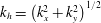 $k_{h}=\left(k_{x}^{2}+k_{y}^{2}\right)^{1/2}$
. Equation (3.2) has been derived from the polarisation relations for hydrostatic IGWs (see equation (10) in Zülicke & Peters (Reference Zülicke and Peters2006) or equation (A4) in Marks & Eckermann (Reference Marks and Eckermann1995)). It is assumed that the divergence is mainly unbalanced and resembles IGW modes. For a local phase-independent estimate of its variance (equal to half of the squared amplitude) and the related horizontal wavenumber the Hilbert transform is used to give
 $$\begin{eqnarray}e=\frac{1}{2}\frac{A[\unicode[STIX]{x1D6FF}]^{2}}{k_{x}[\unicode[STIX]{x1D6FF}]^{2}+k_{y}[\unicode[STIX]{x1D6FF}]^{2}}.\end{eqnarray}$$
The results are compiled in table 3. In order to simplify the comparison with laboratory data, we provide wavelengths
 $\unicode[STIX]{x1D706}=2\unicode[STIX]{x03C0}/|\boldsymbol{k}|$
instead of wavenumbers. Furthermore, figure 10 presents horizontal cross-sections of the weighted amplitude
 $A$
(2.66) (a) and of the wavelengths
 $\unicode[STIX]{x1D706}$
(b). The four earlier defined wave packets (WP1–WP4) are highlighted. Considering the wave parameters in table 3, WP2 located at the pressure minimum is the strongest WP in amplitude and therefore in energy. The wave diagnosis shows the difference between WP1 and WP3 by the wavenumber in the
 $y$
-direction
 $k_{y}$
underlining the different orientation of the two wave packets. WP4 shows the highest wavelength.
Wave diagnosis output of rotating annulus experiment: horizontal cross-sections (at
 $z=3~\text{cm}$
) of amplitude
 $A$
in
 $\text{s}^{-1}$
(a) and wavelength
 $\unicode[STIX]{x1D706}$
in cm (b). The locations of four different wave packets (WP1–WP4) are highlighted.

Tabular overview of the wave parameters of WP1, WP2, WP3 and WP4 calculated by the wave diagnosis.

3.3 Tangent-linear simulations
In this section the influence of the forcing by the internal balanced flow on the IGW field is investigated and compared to the generation by boundary-layer instabilities. The tangent-linear model is therefore integrated with this forcing. To suppress the effect of boundary-layer dynamics, the window function (2.57) is applied at every time step. With the same purpose we consider the corresponding dynamics in the doubly periodic Cartesian set-up without side walls. Given a state from the fully nonlinear simulation, separated into the balanced and unbalanced parts for initialisation of the tangent-linear model, two different initial states are chosen for the unbalanced part of the flow. First, the unbalanced part is set to zero at
 $t=0~\text{s}$
to focus on the development of the unbalanced flow radiated spontaneously by the geostrophically and hydrostatically balanced part. Second, the tangent-linear model is initialised with the unchanged unbalanced part, to observe how its structure develops with and without the balanced forcing.
Horizontal cross-sections (at
 $z=3~\text{cm}$
) of the geostrophically and hydrostatically balanced forcing terms for the annulus model at initial time
 $t=0~\text{s}$
: see (2.33) and (2.34). Forcing of (a) unbalanced zonal velocity
 $u_{u}$
(in
 $\text{cm}~\text{s}^{-2}$
), (b) unbalanced radial velocity
 $v_{u}$
(in
 $\text{cm}~\text{s}^{-2}$
) and (c) unbalanced buoyancy
 $B_{u}$
(in
 $\text{cm}~\text{s}^{-3}$
).

Unbalanced horizontal velocity divergence in the annulus (at
 $z=3~\text{cm}$
) of (a) the nonlinear model and (b) the tangent-linear model. Results are shown 20 s after the initialisation of the tangent-linear simulation with zero unbalanced part. The location of wave packets is highlighted by WP1–WP4 for the nonlinear and WP1
 $^{\prime }$
, WP2
 $^{\prime }$
, WP4
 $^{\prime }$
for the linear model. WP3 is not existent in the tangent-linear model. Units in
 $\text{s}^{-1}$
.

3.3.1 Initially vanishing unbalanced flow part
First, we present the results of the tangent-linear simulations starting with vanishing unbalanced flow part. By initialising the linear model with zero unbalanced part we can focus on two aspects. First, we can verify whether the forced tangent-linear model is capable of reproducing the signal seen in the fully nonlinear simulations, to justify the main assumptions made in the derivation of the tangent-linear model, namely the smallness of the unbalanced fields compared to the balanced fields and the neglect of the nonlinear unbalanced terms. Second, we can quantify the contribution of the purely balanced, nonlinear forcing terms on the right-hand side of the linear system. Only these terms initially contribute to the time evolution of the unbalanced fields and therefore their role as an IGW source can be quantified. Figure 11(a–c) illustrates the horizontal structure of the forcing terms (2.33) and (2.34) included in the zonal (azimuthal) and meridional (radial) momentum and in the buoyancy equation (2.48)–(2.50). In general, all fields consist of rather large-scale patterns with relatively large amplitudes around the pressure minimum. Moreover, the signal of the couplet of horizontal divergence is clearly visible left of the low pressure centre, particularly in the forcing of the buoyancy (figure 11
c). The forcing terms exhibit typical (rotated) dipole structures at both locations and the amplitudes of the forcing of the horizontal velocity components are of the same order. A similar situation is found in the vortex-dipole study of Snyder et al. (Reference Snyder, Plougonven and Muraki2009), where large-scale patterns also only exist in the centre of the vortex dipole in the case of the horizontal velocity and the potential temperature forcing. The amplitudes of the velocity forcings are also of the same order; however, the fields show tripolar or even quadrupolar structures. The results of the tangent-linear simulations are shown in figure 12 in the form of the unbalanced horizontal velocity divergence of the full (figure 12
a) and the linear model (figure 12
b). The fields are plotted after
 $t=20~\text{s}$
of integration time when there is maximum agreement between the full and the linear fields. Wave packet WP1 which is observed in the full model also appears in the tangent-linear simulations where it is highlighted by WP1
 $^{\prime }$
. Furthermore, the tangent-linear simulations show wave activity at the pressure minimum, referred to as WP2
 $^{\prime }$
. WP3 is not existent in the tangent-linear configuration. Wave packet WP4 also develops in the tangent-linear model (WP4
 $^{\prime }$
), even if the wave amplitude is weaker compared to the full model.
Although the extent of WP1
 $^{\prime }$
is shorter than that of WP1 and the wave amplitudes are slightly overestimated, the reproducibility of WP1 by the linear model implies that the ascent–descent couplet also develops in the linear dynamics. The spiral structure of WP2
 $^{\prime }$
is more pronounced than in the full model (WP2), indicating a stronger vortex structure simulated by the linear model. The explanation for the absence of WP3 in the linear model is that it is generated by boundary-layer instabilities occurring at the inner side wall of the annulus and propagates into the interior of the domain. As mentioned in § 1, proposed generation mechanism for the radiation of such waves are, for instance, discussed in Jacoby et al. (Reference Jacoby, Read, Williams and Young2011) and Randriamampianina & Crespo del Arco (Reference Randriamampianina and Crespo del Arco2015). Due to the application of the window function implemented in our linear model (see § 2.2.3) we suppress these processes. Consequently, such wave packets cannot be found in the linear simulations. Likewise, the development of WP4
 $^{\prime }$
at the jet stream near the outer cylinder wall is affected by the window function resulting in weaker amplitudes. The fact that WP1 and, to some extent, WP2 and WP4 also form in the forced linear model supports the assumption that part of the IGWs observed in the rotating annulus experiment actually originate from the jet–front system and not from boundary-layer instabilities. Since we initialise our linear equations with a vanishing unbalanced part we can explicitly show that the balanced forcing terms induce the generation of the IGWs. The different structure and amplitude of WP2
 $^{\prime }$
might be explained by two main reasons. As shown in § 3.2.2, WP2 exhibits the largest amplitude of all WPs. Therefore, nonlinear self-interactions might play an important role in shaping WP2. In addition, quasi-geostrophic theory is assumed to be less accurate for a flow with relatively strongly curved trajectories (e.g. Fultz Reference Fultz1991; Warn et al.
Reference Warn, Bokhove, Shepherd and Vallis1995; Zhang et al.
Reference Zhang, Koch, Davis and Kaplan2000), a circumstance which is present for the vortex observed in our study. And indeed, we observe that the band of relatively strong velocity amplitude around the pressure minimum (see figure 4
c) is less well reproduced in
 $\boldsymbol{u}_{\boldsymbol{b}}$
than other regions of the velocity field (not shown). In order to underpin the previous statements, we consider the results obtained from the modified Cartesian, doubly periodic model. In this case boundary-layer effects from side walls can definitely be excluded. As initial state we use the simulation output described in § 3.1.2 showing a fully baroclinic-wave structure along with already pronounced IGW signals. The results which are most illustrative after
 $t=5~\text{s}$
of integration time are provided in figure 13 where horizontal cross-sections of the horizontal divergence of the nonlinear (figure 13
a) and the forced linear model (figure 13
b) are displayed. In principle, the full model exhibits two wave packets, WPC1 and WPC2, each appearing at the temperature fronts in the region with the maximum horizontal wind speeds (see figure 6). The tangent-linear simulation results show very good agreement. The two wave packets are captured well in both location and amplitude. Since there are only minor differences in the two divergence fields, the capabilities of the tangent-linear model to simulate the dynamics seen in the full system are supported once more. Moreover, the results strengthen the assumption that part of the IGWs observed in the annulus actually come from the dynamics taking place in the inner region which is unaffected by cylinder walls.
Unbalanced horizontal velocity divergence (in
 $\text{s}^{-1}$
) in the Cartesian model configuration (at
 $z=3~\text{cm}$
) of (a) the nonlinear model and (b) the tangent-linear model. Results are shown 5 s after starting the linear simulation with zero unbalanced part. Location of wave packets are highlighted by WPC1 and WPC2 for the nonlinear and WPC1
 $^{\prime }$
and WPC2
 $^{\prime }$
for the linear model.

Time series of the volume average of the horizontal divergence
 $\unicode[STIX]{x1D6FF}$
and of the total kinetic energy of the flow
 $E_{kin}$
starting at the same time as the tangent-linear simulations. (a) In the rotating annulus, (b) in the Cartesian model. The time average is subtracted from the kinetic-energy time series.

Unbalanced horizontal velocity divergence (in
 $\text{s}^{-1}$
) in the annulus (at
 $z=3~\text{cm}$
) for different model set-ups. (a,b) Fields of the nonlinear model at (a) initial time
 $t=0~\text{s}$
and (b) after 20 s of integration time. (c,d) Results of the corresponding forced (c) and unforced (d) linear simulations after 20 s of integration time. All simulations are initialised with the same unbalanced field shown in (a). Location of wave packets is highlighted by WP1–WP4 for the nonlinear, WP1
 $^{\prime }$
–WP3
 $^{\prime }$
for the forced linear and by WP1
 $^{\prime \prime }$
–WP3
 $^{\prime \prime }$
for the unforced linear model. WP4 is hardly identifiable in the tangent-linear configurations. The Pearson correlation coefficient showing the correlation between the two linear and the nonlinear horizontal cross-sections can be found in the lower right corner.

The wave packets presented here are emitted during a baroclinic-wave life cycle and are eventually dissipated. New wave packets are emitted during each life cycle, as long as they present the required forcing properties. We can illustrate this somewhat periodic emission, and then dissipation, of IGW following the life cycles by considering the time series of the volume-averaged horizontal divergence in view of the total kinetic energy of the flow, sampled during the direct numerical simulations. The first quantity indicates the amount of IGW activity while the second points to the state of the large-scale flow. In the annulus configuration, this shows a surge of the IGW activity in the time interval considered for tangent-linear simulations (figure 14
a). The amplitude of IGW activity grows until
 $150~\text{s}$
after the start of tangent-linear simulations and then collapses at
 $200~\text{s}$
, as indicated by the increase, and then decrease, of the volume-averaged horizontal divergence. Visualisations (not shown) indicate that nearly no wave packets are present in the flow in the time interval
 $[200;275]~\text{s}$
. IGW then reappear, concomitantly with the increase of volume-averaged horizontal divergence. The kinetic-energy variations indicate that each of these emission events occur during two successive baroclinic-wave life cycles. The picture is very similar in the Cartesian model simulations. A strong growth of horizontal divergence occurs during the first IGW emission (figure 14
b), studied by tangent linear simulations. We again find a series of successive growth, and then decay, of IGW activity. Note that in the Cartesian configuration, the amplitude of each event decreases cycle after cycle and that the duration over which IGW are emitted is shorter (
 $150~\text{s}$
in annulus simulations versus
 $30~\text{s}$
in Cartesian simulations). We can directly correlate the appearance and increase of IGW activity to the forcing we have identified. There are several other competing effects that lead to them being sustained during a smaller or longer duration. In both cylindrical and Cartesian configurations the relatively high Ekman number means that viscosity (and thermal diffusion) will dissipate the IGW faster than in atmospheric conditions. A stronger shear near the inner wall of the annulus helps to maintain IGW longer in this location, leading to a longer lifetime of each IGW wave packet.
Time evolution of 3-D correlation coefficient between tangent-linear and nonlinear simulations for the annulus model configuration. Solid line: correlation between the nonlinear and the forced linear model. Dashed line: correlation between the nonlinear and the unforced linear model.

3.3.2 Initially non-zero unbalanced part
Next, we perform tangent-linear simulations with an initially non-zero unbalanced state. In addition to the full and the forced linear model simulations, we present results in which the geostrophically and hydrostatically balanced forcing terms are set to zero. It is important to note that in our initial state IGWs already exist within the domain. Thus, the main purpose of this analysis is to compare the influence of the forcing on existing waves. Figure 15(a) shows a cross-section of the horizontal divergence field (at
 $z=3~\text{cm}$
) serving as initial state for all model configurations. The corresponding results after 20 s of integration time are presented in figure 15(b) for the full model, and in figure 15(c,d) for the forced and the unforced tangent-linear model. Additionally, in order to evaluate the linear results more quantitatively, the Pearson correlation coefficients of the (un)forced linear and the full horizontal cross-sections are computed. For this, only those grid points are taken into account which are not affected by the application of the window function (see § 2.2.3). Since these simulations are initialised with identical unbalanced fields, there is a correlation of one between the tangent-linear and the nonlinear fields at the beginning. After 20 s of integration time, the forced tangent-linear model (figure 15
c) shows a correlation of 0.5, whereas the correlation of the unforced model (figure 15
d) is significantly lower (0.2). A particular reason for the lower correlation in the unforced configuration is the more pronounced spiral structure around the pressure minimum compared to the full and the forced tangent-linear models. A time evolution of the 3-D correlation coefficients is provided in figure 16. Compared to the forced annulus simulations (solid line), the correlation of the unforced linear model (dashed line) initially decreases much faster until both curves show a quite similar slope. After approximately
 $t=35~\text{s}$
of integration time, the forced correlation starts to converge towards the unforced one. From this time on, the forced linear fields move clearly away from the dynamics observed in the full model, probably caused by the neglect of the nonlinearities and by the use of the window function.
Wave packets WP1–WP3 can be identified in both linear simulations, labelled with WP1
 $^{\prime }$
–WP3
 $^{\prime }$
in the forced and WP1
 $^{\prime \prime }$
–WP3
 $^{\prime \prime }$
in the unforced tangent-linear configuration (see figure 15). In general, both linear simulations capture the positions, wavelengths and orientations of wave packets WP1 and WP3. However, an amplification of the wave amplitudes can be observed in both systems. The shape of WP2 is still reasonably present in the forced model (WP2
 $^{\prime }$
). In contrast, wave packet WP2
 $^{\prime \prime }$
, which is only affected by the linear operator
 $\boldsymbol{L}_{\boldsymbol{u}}$
, shows clear differences in structure and a significant overestimation of the amplitudes. Hence, WP2 is continuously affected by the balanced part of the flow. As already mentioned in § 3.3.1, the fact that WP4 is hardly identifiable in the (un)forced tangent-linear simulations is again a result of the window function which damps the development of the wave packet. In summary, we can state that the forcing of IGWs by the balanced flow has a significant influence on the time development of the overall structure of WP2, manifested by the much faster decrease in correlation in the unforced model. However, there is only a minor impact on the propagation of the small-scale wave packets WP1 and WP3 which were already present at initial time. This is consistent with the theoretical consideration given in § 2.2.3.
Unfortunately, it is not possible to perform corresponding experiments in the doubly periodic Cartesian configuration. When initialising the model with a non-zero unbalanced field, the linear fields start to diverge after a few seconds of integration time. In particular, we detect unbounded linear instabilities at grid scale. The reason for this is most likely the neglect of the nonlinear terms which leads to an increased energy cascade towards small-scale structures causing exponential growth of the latter. Nevertheless, the results obtained during the short stable time period confirm the results of the annulus investigations. The correlation of the unforced model decreases faster compared to the forced one. Moreover, there seems to be no direct impact on the wave propagation of already existing wave packets which, in this configuration, must have been radiated by the internal flow.
4 Conclusions
This study investigates the role of internal flow dynamics, as opposed to boundary-layer instabilities, in the generation of IGWs observed in numerical simulations of the differentially heated rotating annulus experiment. The focus is on an atmosphere-like configuration of the annulus with a ratio of
 $N/f>1$
(Borchert et al.
Reference Borchert, Achatz and Fruman2014). This set-up of the experiment has not been investigated in the laboratory yet, and it certainly pushes the limits of validity of the Boussinesq approximations. Although we believe that the latter still apply here, final experimental validation is pending, and hence highly desirable. For a clearer view of the internal dynamics, not affected by instabilities at the side wall, we also consider a closely related set-up with doubly periodic horizontal boundary conditions where the baroclinically unstable large-scale state is forced by thermal relaxation.
On the larger scales, our simulations show a baroclinic-wave structure exhibiting a jet–front system similar to its atmospheric counterpart. Additionally, small-scale structures which are associated with IGWs occur in four distinct wave packets in the annulus set-up and in two wave packets in the doubly periodic set-up. These wave packets are diagnosed as part of the unbalanced flow. Here, geostrophic and hydrostatic equilibrium are used as balance concepts, and the balanced flow is obtained by potential vorticity inversion and application of the quasi-geostrophic omega equation. The generation of unbalanced flow is investigated systematically by reformulating the dynamics in terms of an explicit interaction between balanced and unbalanced flow. The balanced forcing of the unbalanced flow is identified, and its effect is studied in tangent-linear models of the unbalanced flow. In these the time-dependent balanced flow is prescribed, as diagnosed from the nonlinear simulations, and all nonlinear self-interactions of the unbalanced flow are neglected. The tangent-linear simulations of the annulus set-up indicate that three wave packets are radiated from the internal flow, whereas a fourth one is most likely generated at the side wall of the annulus. Moreover, it turns out that the forcing of the IGWs by the internal balanced flow significantly contributes to the overall wave generation. The unbalanced flow forced in the doubly periodic set-up very clearly exhibits the same structure as observed in the wave packets from the nonlinear simulations. The relatively strong temperature contrast between the two side walls might suggest that convective gravity wave generation (e.g. Beres, Alexander & Holton Reference Beres, Alexander and Holton2004; Song & Chun Reference Song and Chun2005) also contributes to the observed signal. We do not see any convective cells in our simulations, however, so this process seems to be excluded.
Our study provides deepened insight into the findings of Borchert et al. (Reference Borchert, Achatz and Fruman2014) who performed simulations in the same annulus configuration. They observe clear IGW signals close to the inner boundary and within the baroclinic wave. Based on our investigations we are now able to assign source regions and corresponding generation mechanisms of the respective wave patterns. In principle, we underpin the assumption made by Borchert et al. (Reference Borchert, Achatz and Fruman2014) that a significant part of the IGWs observed in the simulations actually originates from the jet–front system. Along with the wave pattern arranged around the pressure minimum of the baroclinic wave, we observe additional wave packets developing from a couplet of horizontal divergence, also being generated within the internal flow, and at the jet-stream located near the outer cylinder wall. Without doubt, there is a substantial part of IGWs which is generated at the inner side wall before propagating into the interior of the annulus domain. This mechanism is studied extensively by Jacoby et al. (Reference Jacoby, Read, Williams and Young2011) and Randriamampianina & Crespo del Arco (Reference Randriamampianina and Crespo del Arco2015). However, both of these studies consider a traditional annulus set-up with
 $N/f<1$
.
The internal forcing mechanism considered in our study is due to the balanced flow. We therefore conclude that part of the IGWs are generated continuously from the time-dependent large-scale balanced flow. Our balance concept relies on small Rossby numbers, and partial contribution of higher-order balanced components to our unbalanced flow cannot be excluded. We do observe only modest Rossby numbers, however, so we take the forcing as an indication of spontaneous imbalance (Zhang Reference Zhang2004; Vanneste Reference Vanneste2013). This is interesting not only because the differentially heated rotating annulus experiment allows experimental investigations of this process in the laboratory, but also because it exhibits a more complex, more realistic jet–front system compared to the idealised vortex-dipole studies of Snyder et al. (Reference Snyder, Plougonven and Muraki2009) and Wang & Zhang (Reference Wang and Zhang2010). We hope that the systematic flow and dynamics decomposition employed here can help systematic investigations of IGW radiation by jets and fronts in even more realistic atmospheric simulations, following the overall aim to develop and improve corresponding physically based source parametrisations.
Acknowledgements
The authors thank three reviewers for helpful comments on the manuscript. S.H., S.B., L.S., C.Z. and U.A. thank the German Research Foundation (DFG) for partial support through the research unit FOR 1898 Multiscale Dynamics of Gravity Waves (MS-GWaves) and through grants AC 71/8-1, AC 71/9-1, AC 71/10-1, ZA 268/10-1 and ZU 120/2-1. J.R. thanks the Institut PPrime for support while working on the final version.
Appendix A.
Based on the PV defined in (2.21) we can derive a prognostic equation for the PV as follows:
 $$\begin{eqnarray}\displaystyle \frac{\text{D}\unicode[STIX]{x1D6F1}}{\text{D}t}=\frac{\text{D}\unicode[STIX]{x1D701}}{\text{D}t}+\frac{f}{N^{2}}\frac{\text{D}}{\text{D}t}\left(\frac{\unicode[STIX]{x2202}B}{\unicode[STIX]{x2202}z}\right), & & \displaystyle\end{eqnarray}$$
with
 $f,N^{2}=\text{const}$
. Therein, the material derivative of the vertical component of the vorticity is (Vallis Reference Vallis2006)
 $$\begin{eqnarray}\displaystyle \frac{\text{D}\unicode[STIX]{x1D701}}{\text{D}t}=-(f+\unicode[STIX]{x1D701})\unicode[STIX]{x1D6FF}-\frac{\unicode[STIX]{x2202}\boldsymbol{u}}{\unicode[STIX]{x2202}z}\boldsymbol{\cdot }(\boldsymbol{e}_{\boldsymbol{z}}\times \unicode[STIX]{x1D735}_{\boldsymbol{h}}w) & & \displaystyle\end{eqnarray}$$
 $$\begin{eqnarray}\displaystyle \frac{\text{D}}{\text{D}t}\left(\frac{\unicode[STIX]{x2202}B}{\unicode[STIX]{x2202}z}\right)=\left(N^{2}+\frac{\unicode[STIX]{x2202}B}{\unicode[STIX]{x2202}z}\right)\unicode[STIX]{x1D6FF}-\frac{\unicode[STIX]{x2202}\boldsymbol{u}}{\unicode[STIX]{x2202}z}\boldsymbol{\cdot }\unicode[STIX]{x1D735}_{\boldsymbol{h}}B. & & \displaystyle\end{eqnarray}$$
As a result we obtain
 $$\begin{eqnarray}\displaystyle \frac{\text{D}\unicode[STIX]{x1D6F1}}{\text{D}t}=-\left(\unicode[STIX]{x1D701}-\frac{f}{N^{2}}\frac{\unicode[STIX]{x2202}B}{\unicode[STIX]{x2202}z}\right)\unicode[STIX]{x1D6FF}-\frac{\unicode[STIX]{x2202}\boldsymbol{u}}{\unicode[STIX]{x2202}z}\boldsymbol{\cdot }\left(\boldsymbol{e}_{\boldsymbol{z}}\times \unicode[STIX]{x1D735}_{\boldsymbol{h}}w+\frac{f}{N^{2}}\unicode[STIX]{x1D735}_{\boldsymbol{h}}B\right). & & \displaystyle\end{eqnarray}$$
Appendix B.
Here, we extract the purely balanced part in
 $\text{D}\boldsymbol{u}_{\boldsymbol{b}}/\text{D}t$
and
 $\text{D}B_{b}/\text{D}t$
as it is required as forcings in the tangent-linear model in § 2.2.3. Therefore, we apply the material derivative to (2.19) and (2.20) which gives
 $$\begin{eqnarray}\displaystyle & \displaystyle \frac{\text{D}\boldsymbol{u}_{\boldsymbol{b}}}{\text{D}t}=\frac{1}{f}\boldsymbol{e}_{\boldsymbol{z}}\times \left(\frac{\text{D}}{\text{D}t}\unicode[STIX]{x1D735}_{\boldsymbol{h}}p_{b}\right)=\frac{1}{f}\boldsymbol{e}_{\boldsymbol{z}}\times \left(\unicode[STIX]{x1D735}_{\boldsymbol{h}}\frac{\text{D}p_{b}}{\text{D}t}-\unicode[STIX]{x1D735}_{\boldsymbol{h}}\boldsymbol{v}\boldsymbol{\cdot }\unicode[STIX]{x1D735}p_{b}\right) & \displaystyle\end{eqnarray}$$
 $$\begin{eqnarray}\displaystyle & \displaystyle \frac{\text{D}B_{b}}{\text{D}t}=\frac{\text{D}}{\text{D}t}\frac{\unicode[STIX]{x2202}p_{b}}{\unicode[STIX]{x2202}z}=\frac{\unicode[STIX]{x2202}}{\unicode[STIX]{x2202}z}\left(\frac{\text{D}p_{b}}{\text{D}t}\right)-\frac{\unicode[STIX]{x2202}\boldsymbol{v}}{\unicode[STIX]{x2202}z}\boldsymbol{\cdot }\unicode[STIX]{x1D735}p_{b}. & \displaystyle\end{eqnarray}$$
To obtain an expression for
 $\text{D}p_{b}/\text{D}t$
we first consider
 $$\begin{eqnarray}\displaystyle \unicode[STIX]{x1D735}_{\boldsymbol{q}\boldsymbol{g}}\frac{\text{D}p_{b}}{\text{D}t} & = & \displaystyle \frac{\unicode[STIX]{x2202}}{\unicode[STIX]{x2202}t}\unicode[STIX]{x1D735}_{\boldsymbol{q}\boldsymbol{g}}p_{b}+\unicode[STIX]{x1D735}_{\boldsymbol{q}\boldsymbol{g}}\left(\boldsymbol{v}\boldsymbol{\cdot }\unicode[STIX]{x1D735}p_{b}\right)\nonumber\\ \displaystyle & = & \displaystyle \frac{\unicode[STIX]{x2202}}{\unicode[STIX]{x2202}t}\unicode[STIX]{x1D735}_{\boldsymbol{q}\boldsymbol{g}}p_{b}+\unicode[STIX]{x1D735}_{\boldsymbol{q}\boldsymbol{g}}\boldsymbol{v}\boldsymbol{\cdot }\unicode[STIX]{x1D735}p_{b}+(\boldsymbol{v}\boldsymbol{\cdot }\unicode[STIX]{x1D735})\unicode[STIX]{x1D735}_{\boldsymbol{q}\boldsymbol{g}}p_{b}\nonumber\\ \displaystyle & = & \displaystyle \frac{\text{D}}{\text{D}t}\unicode[STIX]{x1D735}_{\boldsymbol{q}\boldsymbol{g}}p_{b}+\unicode[STIX]{x1D735}_{\boldsymbol{q}\boldsymbol{g}}\boldsymbol{v}\boldsymbol{\cdot }\unicode[STIX]{x1D735}p_{b}\end{eqnarray}$$
and then we calculate
 $$\begin{eqnarray}\displaystyle \unicode[STIX]{x1D6FB}_{qg}^{2}\frac{\text{D}p_{b}}{\text{D}t}=\unicode[STIX]{x1D735}_{\boldsymbol{q}\boldsymbol{g}}\boldsymbol{\cdot }\unicode[STIX]{x1D735}_{\boldsymbol{q}\boldsymbol{g}}\frac{\text{D}p_{b}}{\text{D}t}=\unicode[STIX]{x1D735}_{\boldsymbol{q}\boldsymbol{g}}\boldsymbol{\cdot }\frac{\text{D}}{\text{D}t}\unicode[STIX]{x1D735}_{\boldsymbol{q}\boldsymbol{g}}p_{b}+\unicode[STIX]{x1D735}_{\boldsymbol{q}\boldsymbol{g}}\boldsymbol{\cdot }(\unicode[STIX]{x1D735}_{\boldsymbol{q}\boldsymbol{g}}\boldsymbol{v}\boldsymbol{\cdot }\unicode[STIX]{x1D735}p_{b}). & & \displaystyle\end{eqnarray}$$
The first term on the right-hand side can be written as
 $$\begin{eqnarray}\displaystyle \unicode[STIX]{x1D735}_{\boldsymbol{q}\boldsymbol{g}}\boldsymbol{\cdot }\frac{\text{D}}{\text{D}t}\unicode[STIX]{x1D735}_{\boldsymbol{q}\boldsymbol{g}}p_{b} & = & \displaystyle \frac{\unicode[STIX]{x2202}}{\unicode[STIX]{x2202}t}\unicode[STIX]{x1D6FB}_{qg}^{2}p_{b}+\unicode[STIX]{x1D735}_{\boldsymbol{q}\boldsymbol{g}}\boldsymbol{\cdot }(\boldsymbol{v}\boldsymbol{\cdot }\unicode[STIX]{x1D735}\unicode[STIX]{x1D735}_{\boldsymbol{q}\boldsymbol{g}}p_{b})\nonumber\\ \displaystyle & = & \displaystyle \frac{\unicode[STIX]{x2202}}{\unicode[STIX]{x2202}t}\unicode[STIX]{x1D6FB}_{qg}^{2}p_{b}+\unicode[STIX]{x1D735}_{\boldsymbol{q}\boldsymbol{g}}\boldsymbol{v}\boldsymbol{\cdot }\boldsymbol{\cdot }\,\unicode[STIX]{x1D735}\unicode[STIX]{x1D735}_{\boldsymbol{q}\boldsymbol{g}}p_{b}+(\boldsymbol{v}\boldsymbol{\cdot }\unicode[STIX]{x1D735})\unicode[STIX]{x1D6FB}_{qg}^{2}p_{b}\nonumber\\ \displaystyle & = & \displaystyle \frac{\text{D}}{\text{D}t}\unicode[STIX]{x1D6FB}_{qg}^{2}p_{b}+\unicode[STIX]{x1D735}_{\boldsymbol{q}\boldsymbol{g}}\boldsymbol{v}\boldsymbol{\cdot }\boldsymbol{\cdot }\,\unicode[STIX]{x1D735}\unicode[STIX]{x1D735}_{\boldsymbol{q}\boldsymbol{g}}p_{b}\end{eqnarray}$$
and the second as
 $$\begin{eqnarray}\displaystyle \unicode[STIX]{x1D735}_{\boldsymbol{q}\boldsymbol{g}}\boldsymbol{\cdot }(\unicode[STIX]{x1D735}_{\boldsymbol{q}\boldsymbol{g}}\boldsymbol{v}\boldsymbol{\cdot }\unicode[STIX]{x1D735}p_{b})=\unicode[STIX]{x1D6FB}_{qg}^{2}\boldsymbol{v}\boldsymbol{\cdot }\unicode[STIX]{x1D735}p_{b}+\unicode[STIX]{x1D735}_{\boldsymbol{q}\boldsymbol{g}}\boldsymbol{v}\boldsymbol{\cdot }\boldsymbol{\cdot }\,\unicode[STIX]{x1D735}\unicode[STIX]{x1D735}_{\boldsymbol{q}\boldsymbol{g}}p_{b}, & & \displaystyle\end{eqnarray}$$
where
 $\boldsymbol{\cdot }\boldsymbol{\cdot }$
denotes the double scalar product. Given two dyads
 $\boldsymbol{a}\boldsymbol{b}$
and
 $\boldsymbol{c}\boldsymbol{d}$
, with
 $\boldsymbol{a}$
,
 $\boldsymbol{b}$
,
 $\boldsymbol{c}$
and
 $\boldsymbol{d}$
being arbitrary vectors, their double scalar product is defined as (Zdunkowski & Bott Reference Zdunkowski and Bott2003)
 $$\begin{eqnarray}\displaystyle \boldsymbol{a}\boldsymbol{b}\boldsymbol{\cdot }\boldsymbol{\cdot }\,\boldsymbol{c}\boldsymbol{d}=\left(\boldsymbol{b}\boldsymbol{\cdot }\boldsymbol{c}\right)\left(\boldsymbol{a}\boldsymbol{\cdot }\boldsymbol{d}\right)=\boldsymbol{a}\boldsymbol{\cdot }\left(\boldsymbol{b}\boldsymbol{\cdot }\boldsymbol{c}\boldsymbol{d}\right)=\left(\boldsymbol{a}\boldsymbol{b}\boldsymbol{\cdot }\boldsymbol{c}\right)\boldsymbol{\cdot }\boldsymbol{d}=\left(\boldsymbol{d}\boldsymbol{\cdot }\boldsymbol{a}\right)\left(\boldsymbol{c}\boldsymbol{\cdot }\boldsymbol{b}\right)=\boldsymbol{c}\boldsymbol{d}\boldsymbol{\cdot }\boldsymbol{\cdot }\,\boldsymbol{a}\boldsymbol{b}. & & \displaystyle\end{eqnarray}$$
Furthermore, given an arbitrary normal basis
 $\boldsymbol{e}_{\boldsymbol{i}}$
,
 $i=1,2,3$
, in which two tensors
 $\unicode[STIX]{x1D63C}$
and
 $\unicode[STIX]{x1D63D}$
are measured,
 $\unicode[STIX]{x1D63C}=\unicode[STIX]{x1D608}_{ij}\boldsymbol{e}_{\boldsymbol{i}}\boldsymbol{e}_{\boldsymbol{j}}$
and
 $\unicode[STIX]{x1D63D}=\unicode[STIX]{x1D609}_{kl}\boldsymbol{e}_{\boldsymbol{k}}\boldsymbol{e}_{\boldsymbol{l}}$
, their double scalar product reads
 $$\begin{eqnarray}\displaystyle \unicode[STIX]{x1D63C}\boldsymbol{\cdot }\boldsymbol{\cdot }\,\unicode[STIX]{x1D63D}=\unicode[STIX]{x1D608}_{ij}\unicode[STIX]{x1D609}_{kl}\boldsymbol{e}_{\boldsymbol{i}}\boldsymbol{e}_{\boldsymbol{j}}\boldsymbol{\cdot }\boldsymbol{\cdot }\,\boldsymbol{e}_{\boldsymbol{k}}\boldsymbol{e}_{\boldsymbol{l}}=\unicode[STIX]{x1D608}_{ij}\unicode[STIX]{x1D609}_{kl}\left(\boldsymbol{e}_{\boldsymbol{j}}\boldsymbol{\cdot }\boldsymbol{e}_{\boldsymbol{k}}\right)\left(\boldsymbol{e}_{\boldsymbol{i}}\boldsymbol{\cdot }\boldsymbol{e}_{\boldsymbol{l}}\right)=\unicode[STIX]{x1D608}_{ij}\unicode[STIX]{x1D609}_{ji}. & & \displaystyle\end{eqnarray}$$
In summary we have
 $$\begin{eqnarray}\unicode[STIX]{x1D6FB}_{qg}^{2}\frac{\text{D}p_{b}}{\text{D}t}=\frac{\text{D}}{\text{D}t}\unicode[STIX]{x1D6FB}_{qg}^{2}p_{b}+2\unicode[STIX]{x1D735}_{\boldsymbol{q}\boldsymbol{g}}\boldsymbol{v}\boldsymbol{\cdot }\boldsymbol{\cdot }\,\unicode[STIX]{x1D735}\unicode[STIX]{x1D735}_{\boldsymbol{q}\boldsymbol{g}}p_{b}+\unicode[STIX]{x1D6FB}_{qg}^{2}\boldsymbol{v}\boldsymbol{\cdot }\unicode[STIX]{x1D735}p_{b}\end{eqnarray}$$
so that, with
 $\unicode[STIX]{x1D6FB}_{qg}^{2}p_{b}=f\unicode[STIX]{x1D6F1}$
,
 $$\begin{eqnarray}\frac{\text{D}p_{b}}{\text{D}t}=\unicode[STIX]{x1D6FB}_{qg}^{-2}\left(f\frac{\text{D}\unicode[STIX]{x1D6F1}}{\text{D}t}+2\unicode[STIX]{x1D735}_{\boldsymbol{q}\boldsymbol{g}}\boldsymbol{v}\boldsymbol{\cdot }\boldsymbol{\cdot }\,\unicode[STIX]{x1D735}\unicode[STIX]{x1D735}_{\boldsymbol{q}\boldsymbol{g}}p_{b}+\unicode[STIX]{x1D6FB}_{qg}^{2}\boldsymbol{v}\boldsymbol{\cdot }\unicode[STIX]{x1D735}p_{b}\right).\end{eqnarray}$$
Finally, we can separate the balanced part in
 $\text{D}p_{b}/\text{D}t$
,
 $$\begin{eqnarray}\displaystyle \frac{\text{D}p_{b}}{\text{D}t}=\left(\frac{\text{D}p_{b}}{\text{D}t}\right)_{b}+\left(\frac{\text{D}p_{b}}{\text{D}t}\right)_{u}, & & \displaystyle\end{eqnarray}$$
with
 $$\begin{eqnarray}\displaystyle & \displaystyle \left(\frac{\text{D}p_{b}}{\text{D}t}\right)_{b}=\unicode[STIX]{x1D6FB}_{qg}^{-2}\left(\unicode[STIX]{x1D6FB}_{qg}^{2}\boldsymbol{u}_{\boldsymbol{b}}\boldsymbol{\cdot }\unicode[STIX]{x1D735}_{\boldsymbol{h}}p_{b}\right), & \displaystyle\end{eqnarray}$$
 $$\begin{eqnarray}\displaystyle & \displaystyle \left(\frac{\text{D}p_{b}}{\text{D}t}\right)_{u}=\unicode[STIX]{x1D6FB}_{qg}^{-2}\left(f\frac{\text{D}\unicode[STIX]{x1D6F1}}{\text{D}t}+2\unicode[STIX]{x1D735}_{\boldsymbol{q}\boldsymbol{g}}\boldsymbol{v}_{\boldsymbol{u}}\boldsymbol{\cdot }\boldsymbol{\cdot }\,\unicode[STIX]{x1D735}_{\boldsymbol{q}\boldsymbol{g}}p_{b}+\unicode[STIX]{x1D6FB}_{qg}^{2}\boldsymbol{v}_{\boldsymbol{u}}\boldsymbol{\cdot }\unicode[STIX]{x1D735}p_{b}\right). & \displaystyle\end{eqnarray}$$
Note that
 $\unicode[STIX]{x1D735}_{\boldsymbol{q}\boldsymbol{g}}\boldsymbol{u}_{\boldsymbol{b}}\boldsymbol{\cdot }\boldsymbol{\cdot }\,\unicode[STIX]{x1D735}\unicode[STIX]{x1D735}_{\boldsymbol{q}\boldsymbol{g}}p_{b}$
does not contribute to the balanced part in
 $\text{D}p_{b}/\text{D}t$
. Using
 $$\begin{eqnarray}\displaystyle \boldsymbol{a}\boldsymbol{b}_{\boldsymbol{h}}\boldsymbol{\cdot }\boldsymbol{\cdot }\,\boldsymbol{c}\boldsymbol{d}=\left(\boldsymbol{b}_{\boldsymbol{h}}\boldsymbol{\cdot }\boldsymbol{c}\right)\left(\boldsymbol{a}\boldsymbol{\cdot }\boldsymbol{d}\right)=\left(\boldsymbol{b}_{\boldsymbol{h}}\boldsymbol{\cdot }\boldsymbol{c}_{\boldsymbol{h}}\right)\left(\boldsymbol{a}\boldsymbol{\cdot }\boldsymbol{d}\right)=\boldsymbol{a}\boldsymbol{b}_{\boldsymbol{h}}\boldsymbol{\cdot }\boldsymbol{\cdot }\,\boldsymbol{c}_{\boldsymbol{h}}\boldsymbol{d}, & & \displaystyle\end{eqnarray}$$
where
 $\boldsymbol{b}_{\boldsymbol{h}}$
is an arbitrary horizontal vector, we obtain
 $$\begin{eqnarray}\displaystyle \unicode[STIX]{x1D735}_{\boldsymbol{q}\boldsymbol{g}}\boldsymbol{u}_{\boldsymbol{b}}\boldsymbol{\cdot }\boldsymbol{\cdot }\,\unicode[STIX]{x1D735}\unicode[STIX]{x1D735}_{\boldsymbol{q}\boldsymbol{g}}p_{b} & = & \displaystyle \unicode[STIX]{x1D735}_{\boldsymbol{q}\boldsymbol{g}}\boldsymbol{u}_{\boldsymbol{b}}\boldsymbol{\cdot }\boldsymbol{\cdot }\,\unicode[STIX]{x1D735}_{\boldsymbol{h}}\unicode[STIX]{x1D735}_{\boldsymbol{q}\boldsymbol{g}}p_{b}=\frac{1}{f}\left[\unicode[STIX]{x1D735}_{\boldsymbol{q}\boldsymbol{g}}\left(\boldsymbol{e}_{\boldsymbol{z}}\times \unicode[STIX]{x1D735}_{\boldsymbol{h}}p_{b}\right)\right]\boldsymbol{\cdot }\boldsymbol{\cdot }\,\unicode[STIX]{x1D735}_{\boldsymbol{h}}\unicode[STIX]{x1D735}_{\boldsymbol{q}\boldsymbol{g}}p_{b}\nonumber\\ \displaystyle & = & \displaystyle -\frac{1}{f}(\underbrace{\unicode[STIX]{x1D735}_{\boldsymbol{q}\boldsymbol{g}}\unicode[STIX]{x1D735}_{\boldsymbol{h}}p_{b}}_{\equiv \unicode[STIX]{x1D63C}}\times \boldsymbol{e}_{\boldsymbol{z}})\boldsymbol{\cdot }\boldsymbol{\cdot }\,\unicode[STIX]{x1D735}_{\boldsymbol{h}}\unicode[STIX]{x1D735}_{\boldsymbol{q}\boldsymbol{g}}p_{b}=-\frac{1}{f}\left(\unicode[STIX]{x1D63C}\times \boldsymbol{e}_{\boldsymbol{z}}\right)\boldsymbol{\cdot }\boldsymbol{\cdot }\,\unicode[STIX]{x1D63C}^{\text{T}}.\quad\end{eqnarray}$$
Since a tensor can be formulated as a sum of dyads
 $\unicode[STIX]{x1D63C}=\sum _{i}\boldsymbol{a}_{\boldsymbol{i}}\boldsymbol{b}_{\boldsymbol{i}}$
(compare (B 8)), we can apply (Wilson Reference Wilson1929; Zdunkowski & Bott Reference Zdunkowski and Bott2003)
 $$\begin{eqnarray}\displaystyle \left(\boldsymbol{a}\boldsymbol{b}\times \boldsymbol{c}\right)\boldsymbol{\cdot }\boldsymbol{\cdot }\,\boldsymbol{d}\boldsymbol{e} & = & \displaystyle \left[\left(\boldsymbol{b}\times \boldsymbol{c}\right)\boldsymbol{\cdot }\boldsymbol{d}\right]\left(\boldsymbol{a}\boldsymbol{\cdot }\boldsymbol{e}\right)=-\left[\boldsymbol{d}\boldsymbol{\cdot }\left(\boldsymbol{c}\times \boldsymbol{b}\right)\right]\left(\boldsymbol{a}\boldsymbol{\cdot }\boldsymbol{e}\right)\nonumber\\ \displaystyle & = & \displaystyle -\left[\boldsymbol{b}\boldsymbol{\cdot }\left(\boldsymbol{d}\times \boldsymbol{c}\right)\right]\left(\boldsymbol{a}\boldsymbol{\cdot }\boldsymbol{e}\right)=-\boldsymbol{b}\boldsymbol{\cdot }\left[\left(\boldsymbol{a}\boldsymbol{\cdot }\boldsymbol{e}\right)\left(\boldsymbol{d}\times \boldsymbol{c}\right)\right]=-\boldsymbol{b}\boldsymbol{\cdot }\left[\boldsymbol{a}\boldsymbol{\cdot }\left(\boldsymbol{e}\boldsymbol{d}\times \boldsymbol{c}\right)\right]\nonumber\\ \displaystyle & = & \displaystyle -\boldsymbol{b}\boldsymbol{a}\boldsymbol{\cdot }\boldsymbol{\cdot }\,\left(\boldsymbol{e}\boldsymbol{d}\times \boldsymbol{c}\right)=-\left(\boldsymbol{a}\boldsymbol{b}\right)^{\text{T}}\boldsymbol{\cdot }\boldsymbol{\cdot }\,\left[\left(\boldsymbol{d}\boldsymbol{e}\right)^{\text{T}}\times \boldsymbol{c}\right]\end{eqnarray}$$
to (B 15), which yields
 $$\begin{eqnarray}\displaystyle -\frac{1}{f}\left(\unicode[STIX]{x1D63C}\times \boldsymbol{e}_{\boldsymbol{z}}\right)\boldsymbol{\cdot }\boldsymbol{\cdot }\,\unicode[STIX]{x1D63C}^{\text{T}}=\frac{1}{f}\unicode[STIX]{x1D63C}^{\text{T}}\boldsymbol{\cdot }\boldsymbol{\cdot }\,\left(\unicode[STIX]{x1D63C}\times \boldsymbol{e}_{\boldsymbol{ z}}\right)=\frac{1}{f}\left(\unicode[STIX]{x1D63C}\times \boldsymbol{e}_{\boldsymbol{z}}\right)\boldsymbol{\cdot }\boldsymbol{\cdot }\,\unicode[STIX]{x1D63C}^{\text{T}}, & & \displaystyle\end{eqnarray}$$
where in the last step
 $\unicode[STIX]{x1D63C}\boldsymbol{\cdot }\boldsymbol{\cdot }\,\unicode[STIX]{x1D63D}=\unicode[STIX]{x1D63D}\boldsymbol{\cdot }\boldsymbol{\cdot }\,\unicode[STIX]{x1D63C}$
(compare (B 7)) has been used. The equation (B 17) can only be satisfied if
 $\unicode[STIX]{x1D735}_{\boldsymbol{q}\boldsymbol{g}}\boldsymbol{u}_{\boldsymbol{b}}\boldsymbol{\cdot }\boldsymbol{\cdot }\,\unicode[STIX]{x1D735}\unicode[STIX]{x1D735}_{\boldsymbol{q}\boldsymbol{g}}p_{b}=0$
.



