


1. Introduction
Methods for prediction of instability and transition have evolved considerably during the past several decades. Advances, driven by increases in computer speed and memory, include the availability of high-fidelity direct numerical simulation (DNS) and large-eddy simulation solutions for canonical wall-bounded flows (Sayadi, Hamman & Moin Reference Sayadi, Hamman and Moin2013), the recognition of transient growth (non-modal instability) as a key mechanism and mathematical formulations for optimal disturbances in linear and nonlinear frameworks (Schmid & Henningson Reference Schmid and Henningson2001; Schmid Reference Schmid2007; Kerswell Reference Kerswell2018), and generalization of parallel-flow analysis to global approaches to flows that are inhomogeneous in two or more directions (Theofilis Reference Theofilis2011).
Most of the stability studies concern linearised evolution of perturbations. For stable base flows, the physical mechanisms associated to linear growth mechanisms (modal and non-modal) and receptivity can be clarified by finding initial conditions in the time domain, or volumetric forcings, in the frequency domain, that maximize, for example, the kinetic energy of perturbations (Schmid & Henningson Reference Schmid and Henningson2001). The frequency-space problem is also called linear resolvent analysis or input/output analysis in the literature. In these analyses, adjoint methods are used to maximise a specific cost function. Trefethen et al. (Reference Trefethen, Trefethen, Reddy and Driscoll1993) and Jovanović & Bamieh (Reference Jovanović and Bamieh2005) showed that the computation of the optimal forcings and responses of the resolvent operator extracts the pseudo-resonances of a flow field, that is, the frequencies and spatial distributions of forcings that optimally trigger linear responses in a system. In a set-up where the streamwise direction is also discretised (in addition to the cross-stream direction), accurate methods to extract the optimal features from the global resolvent have first been carried out with time-stepper approaches by Blackburn, Barkley & Sherwin (Reference Blackburn, Barkley and Sherwin2008), Åkervik et al. (Reference Åkervik, Ehrenstein, Gallaire and Henningson2008), Monokrousos et al. (Reference Monokrousos, Åkervik, Brandt and Henningson2010) and more recently with sparse direct LU methods by Sipp et al. (Reference Sipp, Marquet, Meliga and Barbagallo2010), Brandt et al. (Reference Brandt, Sipp, Pralits and Marquet2011), Rigas et al. (Reference Rigas, Schmidt, Colonius and Bres2017), Schmidt et al. (Reference Schmidt, Towne, Rigas, Colonius and Brès2018), Pickering et al. (Reference Pickering, Rigas, Nogueira, Cavalieri, Schmidt and Colonius2020), among others.
Determining the growth of finite-amplitude perturbations is, of course, more challenging. In practice, the direct solution of the three-dimensional (3-D) Navier–Stokes equations in the time domain is most commonly employed. For example, Rist & Fasel (Reference Rist and Fasel1995) and Bake, Meyer & Rist (Reference Bake, Meyer and Rist2002) reproduced experimental results evidencing different forms of transition in the flat-plate boundary layer. More recently, nonlinear transitional mechanisms have been studied by employing gradient-based techniques to find the smallest amplitude optimal initial conditions that trigger transition to turbulence (Biau & Bottaro Reference Biau and Bottaro2009; Cherubini et al. Reference Cherubini, De Palma, Robinet and Bottaro2010, Reference Cherubini, De Palma, Robinet and Bottaro2011; Monokrousos et al. Reference Monokrousos, Bottaro, Brandt, Di Vita and Henningson2011; Pringle, Willis & Kerswell Reference Pringle, Willis and Kerswell2012; Kerswell Reference Kerswell2018; Vavaliaris, Beneitez & Henningson Reference Vavaliaris, Beneitez and Henningson2020). The optimal perturbation is calculated over a finite time interval and the one with the lowest energy is known as the minimal seed in the time domain. Similar methodology has been applied to study the transition mechanisms in thermoacoustic systems (Juniper Reference Juniper2011) and also recently has been extended to compressible flows (Jahanbakhshi & Zaki Reference Jahanbakhshi and Zaki2019; Huang & Hack Reference Huang and Hack2020). The results still depend on the specific metric (cost function) used to measure the growth; common choices include perturbation kinetic energy (Cherubini et al. Reference Cherubini, De Palma, Robinet and Bottaro2011; Pringle et al. Reference Pringle, Willis and Kerswell2012), integral skin friction coefficient (Jahanbakhshi & Zaki Reference Jahanbakhshi and Zaki2019), dissipation (Monokrousos et al. Reference Monokrousos, Bottaro, Brandt, Di Vita and Henningson2011) and mean shear (Karp & Cohen Reference Karp and Cohen2017).
The minimal seed calculations can be compared, in certain cases, against appropriate experimental measurements of finite-amplitude thresholds for transition to turbulence (Peixinho & Mullin Reference Peixinho and Mullin2007, for experimental pipe flow transition). However, by analog with the linear approaches, it is experimentally more natural to model transition from laminar to turbulent flow as a stationary process where disturbances are continually supplied to the system from the environment, i.e. to consider the receptivity problem. For linear growth, this results in the aforementioned resolvent (or input/output) analysis that provides, in the frequency domain, a transfer function between inputs, for example, environmental noise characterised by spatially localised spectral co-variance tensors, and outputs, for example, the structure of the resulting amplified flow structures, and the net gain between them. Given the convective nature of instabilities in spatially developing boundary layer flows, an accurate and practical prediction of the transition location relies on an accurate description of the amplitude and spectral content of the environmental noise and also on the unravelling of the transition mechanisms, typically the most dangerous ones.
In order to deal with finite-amplitude perturbations in the frequency domain, the stability and numerical tools have to be extended to account for nonlinearity. Previous attempts in this regard have been limited to the nonlinear parabolised stability equations (NPSEs, Bertolotti, Herbert & Spalart Reference Bertolotti, Herbert and Spalart1992; Chang & Malik Reference Chang and Malik1994). While such calculations showed good agreement with DNS for the very early stages of transition, they require specific inlet conditions to be specified and these are typically based on modal solutions to the local (parallel) spatial stability problem. Furthermore, numerical instabilities and robustness issues, associated with the minimum step restriction, have limited the applicability of both parabolised stability equations (PSEs) and NPSEs (Towne, Rigas & Colonius Reference Towne, Rigas and Colonius2019), and cast doubt on whether PSEs can be used to identify optimal inlet conditions or volumetric forcing. The aforementioned work on non-modal mechanisms relies on cooperative amplification of modes with disparate wavelengths, which raises further questions about the appropriateness of PSE ansatz.
A natural generalization in order to calculate finite-amplitude perturbations in the frequency domain is to seek solutions to the full Navier–Stokes equations under the form of an expansion consisting of a mean-flow solution, a fundamental mode and  $p$ harmonics of the fundamental, but without the parabolising approximations inherent to PSEs. Such an approach, known in literature as the harmonic balance method (HBM, Fabre et al. Reference Fabre, Citro, Ferreira-Sabino, Bonnefis, Sierra, Giannetti and Pigou2018; Khalil & Grizzle Reference Khalil and Grizzle2002) is a general method to find periodic or quasi-periodic solutions, which are approximated using truncated Fourier expansions. The HBM has been used previously in fluid mechanics primarily in the context of turbomachinery (Hall, Thomas & Clark Reference Hall, Thomas and Clark2002; Gopinath et al. Reference Gopinath, Van Der Weide, Alonso, Jameson, Ekici and Hall2007; Sicot, Dufour & Gourdain Reference Sicot, Dufour and Gourdain2012), where one seeks a mean flow and harmonics associated with the externally imposed blade passing frequency. When used with
 $p=0$, HBM also recovers the self-consistent model introduced by Mantič-Lugo, Arratia & Gallaire (Reference Mantič-Lugo, Arratia and Gallaire2014) and Mantič-Lugo & Gallaire (Reference Mantič-Lugo and Gallaire2016) for the cylinder wake and backstep flow, respectively.
In this paper, using HBM, we explore the optimal nonlinear amplification problem in the frequency domain, and we use the method to identify and analyse transition scenarios for the flat-plate boundary layer. We begin in § 2 by briefly reviewing the literature on boundary layer transition. In § 3 we propose a solution strategy for the following optimisation problem. Given an amplitude  $A$, a time period and spanwise wavelength associated respectively to the fundamental frequency
 $\omega$ and fundamental wavenumber
 $\beta$, we look for a spatial distribution of a time-periodic (of period
 $2{\rm \pi} /\omega$) and spanwise-periodic (of period
 $2{\rm \pi} /\beta$) volumetric forcing of amplitude
 $A$ that triggers a solution maximising the mean skin friction coefficient (integrated over the wall). In § 4 we validate the HBM solver by reproducing a
 $K$-type transition scenario previously studied using DNS (Rist & Fasel Reference Rist and Fasel1995), while in § 5 we validate the optimisation procedure by reproducing previously reported linear optimal solutions. Finally, in § 6 we calculate nonlinear optimal responses and forcings that maximise the skin friction coefficient. By varying
 $A$,
 $\omega$,
 $\beta$ and the forcing component combinations, we identify a range of optimal transition scenarios. We summarise our results in § 7, and discuss prospects for transition prediction using HBM.
2. Boundary layer transition: a brief review
Early studies on zero-pressure gradient boundary layer transition have been mainly focused on the modal amplification of Tollmien–Schlichting (TS) waves. The primary TS waves develop three-dimensional secondary instabilities, and subsequently break down to turbulence. The analysis of transition mechanisms resulting from the secondary instability of TS waves has identified two main routes.
(i) The fundamental
 $K$-type transition, which involves a planar TS wave $(\omega ,0)$ and two oblique waves of the same frequency $(\omega ,\pm \beta )$. Such a resonance has first been evidenced by Klebanoff, Tidstrom & Sargent (Reference Klebanoff, Tidstrom and Sargent1962).
(ii) The subharmonic
$H$-type transition, triggered by a planar TS wave $(\omega ,0)$ and two subharmonic oblique waves $(\omega /2,\pm \beta )$. It has been experimentally observed by Kachanov, Kozlov & Levchenko (Reference Kachanov, Kozlov and Levchenko1977) and Kachanov & Levchenko (Reference Kachanov and Levchenko1984).


In both cases, the oblique waves are strongly amplified, leading to  $\Lambda$-shaped patterns composed of strong longitudinal vortices (Rist & Fasel Reference Rist and Fasel1995; Berlin, Wiegel & Henningson Reference Berlin, Wiegel and Henningson1999; Sayadi et al. Reference Sayadi, Hamman and Moin2013). In the case of
 $H$-type transition, the
 $\Lambda$-patterns are staggered while they are aligned in the case of
 $K$-type transition. In an effort to explain the observed patterns, Herbert (Reference Herbert1988) examined the secondary stability characteristics of the modified periodic flow (Blasius flow with superimposed TS waves) using linear Floquet analysis in a local framework. The analysis showed that the growth of three-dimensional oblique subharmonic frequency waves (seen for
 $H$-type) is favoured over fundamental waves (
 $K$-type).
More recent work shows that disturbances can undergo significant transient growth that leads to faster transition to turbulence, even at subcritical Reynolds numbers, and potentially bypassing transition through TS waves. A linear resolvent analysis for the Blasius boundary layer has been performed by Monokrousos et al. (Reference Monokrousos, Åkervik, Brandt and Henningson2010) to identify optimal forcing in the frequency domain. Peaks of the optimal gain in the frequency/spanwise wavenumber space were linked to modal and non-modal instabilities. The analysis showed that maximum energy amplification is due to steady three-dimensional disturbances. The optimal forcing consists of streamwise vortices (rolls) and the response of streamwise elongated vortices, known as streaks. The amplification is a purely non-modal mechanism through the linear lift-up mechanism (Landahl Reference Landahl1980; Butler & Farrell Reference Butler and Farrell1992). The non-modal analysis also shows that oblique TS waves are more amplified than the two-dimensional (2-D) ones, though these are linearly suboptimal to the aforementioned lift up mechanism.
Due to early observations that streaks can be significantly amplified and provide an alternative bypass route to turbulence, various studies have focused on the secondary instability of boundary layers distorted by streaks. Andersson et al. (Reference Andersson, Brandt, Bottaro and Henningson2001) performed an inviscid, secondary instability analysis of the optimally amplified boundary layer streaks in a linear framework. Depending on the symmetries of the perturbed flow, varicose or sinuous oscillations of the low-speed streaks are possible, with the latter being the most unstable one. Once the streaks reach a certain amplitude and become unstable, breakdown to a turbulent flow is observed (Brandt & Henningson Reference Brandt and Henningson2002; Hack & Zaki Reference Hack and Zaki2014). The sinuous mode has been linked to the spanwise shear which leads to the formation of streamwise vortices around the low-speed streaks. On the other hand, the varicose mode has been associated with wall-normal shear and the formation of symmetric hairpin vortices (Asai, Minagawa & Nishioka Reference Asai, Minagawa and Nishioka2002; Hack & Moin Reference Hack and Moin2018).
An alternative bypass scenario for transition relies on oblique waves (Schmid & Henningson Reference Schmid and Henningson1992). In this scenario, streamwise-aligned vortices are generated by nonlinear interaction between a pair of oblique waves with equal angle but opposite sign in the flow direction (Schmid & Henningson Reference Schmid and Henningson1992; Reddy et al. Reference Reddy, Schmid, Baggett and Henningson1998; Berlin et al. Reference Berlin, Wiegel and Henningson1999). These vortices, in turn, induce streamwise streaks through the lift-up mechanism. The subsequent stages of transition to turbulence are similar to those described previously for the streak breakdown. The initial stages of the nonlinear interaction of the oblique waves have been described also using NPSEs. Chang & Malik (Reference Chang and Malik1994) showed that the oblique waves are a dominant mechanism at low supersonic speeds. Similarly to the incompressible regime, the nonlinear interaction of a pair of oblique waves results in the evolution of a streamwise vortex. This stage was described by a wave–vortex triad consisting of the oblique waves and a streamwise vortex whereby the oblique waves grow linearly while nonlinear effects result in the rapid growth of the vortex mode.
3. Nonlinear input/output analysis: theory and algorithms
In order to extend the linear input/output (resolvent) analysis to finite-amplitude perturbations, we need to proceed in two steps.
(i) Devise a method to find, for a given time- and spanwise-periodic finite-amplitude forcing, a time- and spanwise-periodic solution with the same periods that is a solution to the forced nonlinear Navier–Stokes equations. For this, we will use the HBM framework. The theory and numerical algorithms are presented in § 3.2.
(ii) Devise a method to search, over a fixed set of forcing and response frequencies, for an optimal forcing with a finite overall amplitude,
$A$, that maximises a given cost functional. Similarly to the optimisation strategies followed in the time domain (Kerswell Reference Kerswell2018), we use gradient-based strategies to find local maxima and optimal solutions in a few iterations (§ 3.3).

3.1. Governing equations and computational set-up
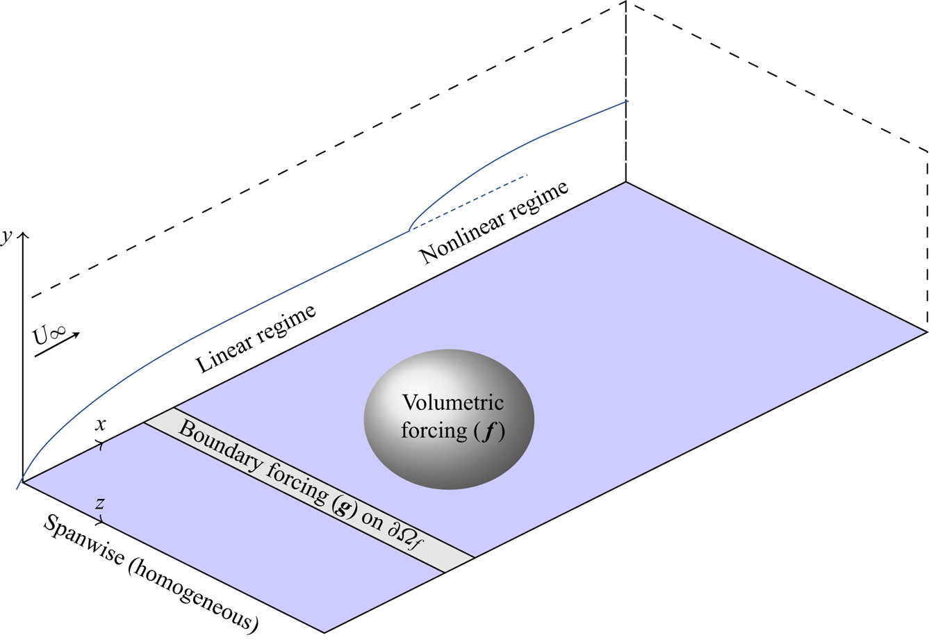
The flow under consideration is the zero-pressure gradient boundary layer flow, shown schematically in figure 1. The spanwise direction  $z$ is treated as homogeneous and, without loss of generality, we will assume that the forcing and response are
 $z$-periodic, in addition to being
 $t$-periodic.
Schematic of the zero-pressure-gradient flat-plate set-up. Transition of the laminar boundary layer is triggered here either by boundary forcing or volumetric momentum forcing. In general, these forcings can model free-stream disturbances or actuators on the boundary/wall (i.e. periodic blowing and suction, vibrating wall, roughness elements) or actuators within the flow (i.e. vibrating ribbon).

We consider the forced three-dimensional incompressible Navier–Stokes equations
 \begin{gather} \partial_t \boldsymbol{u}+\boldsymbol{u}\boldsymbol{\cdot}\boldsymbol{\nabla}\boldsymbol{u}= -\boldsymbol{\nabla} p+\nu{\rm \Delta}\boldsymbol{u}+\boldsymbol{f}(\boldsymbol{x},t), \end{gather}
 \begin{gather}\boldsymbol{\nabla} \boldsymbol{\cdot} \boldsymbol{u}= 0, \end{gather}
 \begin{gather}\boldsymbol{u}=\boldsymbol{g}(\boldsymbol{x},t)\quad \mbox{on}\ \partial \varOmega_f, \end{gather}
where  $\boldsymbol {f}$ is a volumetric time-dependent momentum forcing and
 $\boldsymbol {g}$ a time-dependent forcing on some boundary
 $\partial \varOmega _f$. The forcing terms can represent the effect of free-stream disturbances or actuators on the boundary/wall (i.e. periodic blowing and suction, vibrating wall, roughness elements) or actuators within the flow (i.e. vibrating ribbon).
The governing equations are discretised in the  $x$ and
 $y$ spatial directions, using the finite element method, while
 $z$ and
 $t$ are treated as continuous homogeneous directions. In the discrete state space, the forcing and state variables are then vectors depending only on
 $z$ and
 $t$, while the explicit dependence on
 $x$ and
 $y$ defines the degrees of freedom of the vectors. If we consider the compound state vector
 $\boldsymbol {w}=[\boldsymbol {u},p]$, where
 $\boldsymbol {u}=[u, v, w]$ refers to the
 $x$,
 $y$ and
 $z$ velocity components, the semi-discretized governing equations (3.1) may be recast in the following form:
 \begin{gather} \boldsymbol{M} \partial_t \boldsymbol{w} + \boldsymbol{L}\boldsymbol{w} + \tfrac{1}{2} \boldsymbol{N}(\boldsymbol{w},\boldsymbol{w})= \boldsymbol{MPf}(z,t), \end{gather}
 \begin{gather}P^*w = g(z,t)\quad \mbox{on}\ \partial \varOmega_f. \end{gather}
Here  $\boldsymbol {P}$ is the prolongation matrix mapping a
 $[u,v,w]$ velocity vector into a
 $[u,v,w,0]$ velocity-pressure vector and the transconjugate operator of
 $P$, denoted as
 $P^*$, is the operator transforming a
 $[u,v,w,p]$ vector to
 $[u,v,w]$. The matrices
 $\boldsymbol {M}$,
 $\boldsymbol {L}$ and the bilinear operator
 $\boldsymbol {N}$ are defined as
 \begin{equation} \left.\begin{gathered} \boldsymbol{M}=\left( \begin{array}{cc} \boldsymbol{M}' & \boldsymbol{0} \\ \boldsymbol{0} & 0 \end{array} \right), \quad \boldsymbol{L}=\left( \begin{array}{cc} -\nu \Delta () & \boldsymbol{\nabla}() \\ \boldsymbol{\nabla} \boldsymbol{\cdot} () & 0 \end{array} \right), \\ \boldsymbol{N}(\boldsymbol{w}_1,\boldsymbol{w}_2)= \left( \begin{array}{c} \boldsymbol{u}_1 \boldsymbol{\cdot} \boldsymbol{\nabla} \boldsymbol{u}_2+\boldsymbol{u}_2 \boldsymbol{\cdot} \boldsymbol{\nabla} \boldsymbol{u}_1 \\ 0 \end{array}\right), \end{gathered}\right\} \end{equation}
where  $\boldsymbol {M}$ and
 $\boldsymbol {M}'$ are the mass matrices associated to the spatial discretisation,
 $\boldsymbol {L}$ the Stokes operator and
 $\boldsymbol {N}$ the symmetrised nonlinear convection operator.
We apply no-slip boundary conditions along the plate and zero stress conditions at the outlet. At the inlet and at the upper boundary, we impose the Blasius profile. We consider the free-stream velocity  $U_\infty$ and
 $\nu /U_\infty$ as reference velocity and length scales throughout the manuscript. For this specific choice, we have
 $x \mapsto Re_x$.
The computational domain for the zero-pressure flat-plate configuration is rectangular with the plate located at  $y=0$, the upper boundary at
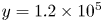 $y=1.2\times 10^{5}$ and the inlet at
 $x_i=0.30\times 10^{5}$. The outlet is at
 $x_o=2.52\times 10^{5}$ (§ 4) or
 $x_o=3.60\times 10^{5}$ (§§ 5 and 6). The inlet Reynolds number based on the displacement thickness,
 $Re_{\delta ^{*}} = 1.72 \sqrt {Re_x}$, is 298, which is subcritical with respect to the local modal instability of planar TS waves,
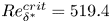 $Re_{\delta ^{*}}^{crit}=519.4$ (Schmid & Henningson Reference Schmid and Henningson2001). The elements close to the plate are based on split rectangular elements, which exhibit a uniform streamwise length of
 ${\rm \Delta} x=400$ and a height at the plate of
 ${\rm \Delta} y = 40$. The height of the split rectangles is stretched in the vertical direction by a factor 1.04 up to the point where the rectangles become squares. From this height, the mesh is gradually stretched isotropically up to the upper boundary.
The discretization is carried out with the FreeFem $++$ software (Hecht Reference Hecht2012), with first-order
 $[P_{1b},P_{1b},P_{1b},P_{1}]$ (Mini) elements (Arnold, Brezzi & Fortin Reference Arnold, Brezzi and Fortin1984) for a
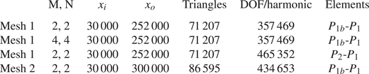
 $\boldsymbol {w}=[u,v,w,p]$ element. The resulting degrees of freedom (DOFs) for the 2-D discretisation of the equations are given in table 1.
Parameters for flat-plate boundary layer computational set-up.

3.2. Nonlinear input/output relation in frequency space with harmonic balance method
The volume  $\boldsymbol {f}(z,t)$ and boundary
 $\boldsymbol {g}(z,t)$ forcings are assumed to be
 $z$-periodic of wavelength
 $\lambda = 2{\rm \pi} / \beta$ and
 $t$-periodic of period
 $T=2{\rm \pi} /\omega$. We assume that the state vector
 $\boldsymbol {w}(z,t)$ behaves the same way. When considering boundary layers in early stage transition, i.e with weak external forcing amplitude, it is reasonable to assume that the response of the system follows the time periodicity and spatial symmetries of the external forcing. A Fourier expansion is introduced for the periodic forcing and state variables, which is truncated at
 $M+1$ harmonics in
 $z$ and
 $N+1$ harmonics in
 $t$. Hence,
 \begin{equation} \boldsymbol{w}(z,t) =\sum_{\substack{-M \leqslant m \leqslant M\\ -N \leqslant n \leqslant N}} \exp({\textrm{i}(m\beta z+n\omega t)}) \hat{\boldsymbol{w}}_{mn}, \end{equation}
with similar expansions (not shown here) for  $\boldsymbol {f}(z,t)$ and
 $\boldsymbol {g}(z,t)$. Term
 $\hat {\boldsymbol {w}}_{mn}$ (respectively
 $\skew3\hat{\boldsymbol{f}}_{mn}$,
 $\hat {\boldsymbol {g}}_{mn}$) represents the harmonic associated to
 $\exp ({\textrm {i}m\beta z+\textrm {i}n\omega t})$ for
 $\hat {\boldsymbol {w}}$ (respectively
 $\skew3\hat{\boldsymbol{f}}$ and
 $\hat {\boldsymbol {g}}$). For these variables to be real, the relation
 \begin{equation} \hat{\boldsymbol{w}}_{-m,-n}=\overline{\hat{\boldsymbol{w}}_{mn}} \end{equation}
must hold for all  $(m,n)$, which induces that
 $\hat {\boldsymbol {w}}_{00}$ is real. The overbar
 $\overline {(\cdot )}$ denotes the complex conjugate. For a high forcing amplitude, quasi-periodic limit cycles may appear, which can be captured by introducing two or more incommensurate fundamental frequencies and their harmonics in expansion (3.4), an investigation which is beyond the scope of the present paper.
After substituting the Fourier expansion (3.4) in the Navier–Stokes equations (3.2), a set of nonlinear equations is obtained by balancing the amplitudes of like harmonics. Specific simple examples are given in § 3.2.1. In the general case, this procedure yields the harmonic-balances Navier–Stokes (HBNS) equations, described by the system of coupled equations
 \begin{gather} \left[ \textrm{i}n\omega \boldsymbol{M} + \boldsymbol{L}_m + \gamma_{00}^{mn} \boldsymbol{N}_0^{m} (\hat{\boldsymbol{w}}_{00}, \cdot) \right]\hat{\boldsymbol{w}}_{mn} +\sum_{\mathcal{S}(m,n)} \gamma_{m_1n_1}^{m_2n_2}\boldsymbol{N}_{m_1}^{m_2} (\hat{\boldsymbol{w}}_{m_1n_1},\hat{\boldsymbol{w}}_{m_2n_2}) = \boldsymbol{M}\boldsymbol{P}\,\hat{\boldsymbol{f}}_{mn}, \end{gather}
 \begin{gather}\boldsymbol{P}^*\hat{\boldsymbol{w}}_{mn} =\hat{\boldsymbol{g}}_{mn} \quad \mbox{on}\ \partial \varOmega_f , \end{gather}
for all  $(m,n)$ such that
 $-M \leqslant m \leqslant M$ and
 $-N \leqslant n \leqslant N$, and the sum is over the set of indices
 \begin{equation} \mathcal{S}(m,n) {\,=\,}\! \left. \begin{cases} m{\,=\,} m_1 + m_2, & -M \leqslant m_1 \leqslant m_2 \leqslant M, \\ n {\,=\,} n_1+n_2, & -N \leqslant n_1 \leqslant n_2 \leqslant N, \end{cases} \right| (m_1,n_1) \ne (0,0), (m_2,n_2) \ne (0,0). \end{equation}
The coefficients  $\gamma _{m_1n_1}^{m_2n_2}=0.5$ if
 $(m_1=m_2,n_1=n_2)$ and
 $1$ in the other cases. The linear matrix
 $\boldsymbol {L}_{m}$ and bilinear operator
 $\boldsymbol {N}_{m_1}^{m_2}$ are deduced from
 $\boldsymbol {L}$ and
 $\boldsymbol {N}$ by replacing
 $\partial _z$ derivatives by
 $\textrm {i}m\beta z$. We define the solution and forcing vectors,
 $\hat {\boldsymbol {w}}$,
 $\skew3\hat{\boldsymbol{f}}$ and
 $\hat {\boldsymbol {g}}$ whose elements correspond to the
 $(2M+1)\times (2N+1)$ complex unknowns.
Then, (3.6) may be rewritten in compact form as
 \begin{gather} \boldsymbol{R}(\hat{\boldsymbol{w}})=\boldsymbol{M}\boldsymbol{P}\,\hat{\boldsymbol{f}}, \end{gather}
 \begin{gather}\boldsymbol{P}^*\hat{\boldsymbol{w}}=\hat{\boldsymbol{g}} \quad \mbox{on}\ \partial \varOmega_f, \end{gather}
where we reuse the symbols  $\boldsymbol {M}$ and
 $\boldsymbol {P}$ to now refer to block matrices composed from the individual equations. For given forcing terms
 $\skew3\hat{\boldsymbol{f}}$ and
 $\hat {\boldsymbol {g}}$, (3.8) are
 $(2M+1)\times (2N+1)$ complex nonlinear equations for the unknowns
 $\hat {\boldsymbol {w}}$. Due to the fact that the equation governing the
 $(m,n)$ harmonic of
 $\hat {\boldsymbol {w}}$ corresponds to the complex conjugate of the equation governing the
 $(-m,-n)$ harmonic, the solution will be symmetric,
 $\hat {\boldsymbol {w}}_{-m,-n}=\overline {\hat {\boldsymbol {w}}_{mn}}$, whenever the forcing is.
3.2.1. Special cases
In order to get some insight into the structure of the governing equations, we consider two particular cases where the boundary forcing term,  $\hat {\boldsymbol {g}}$, is set to zero for simplicity.
In the case where  $M=N=1$, (3.6) reduce to
 \begin{gather} \left[ \boldsymbol{L}_0 + \tfrac{1}{2}\boldsymbol{N}_0^{0} (\hat{\boldsymbol{w}}_{00}, \cdot) \right]\hat{\boldsymbol{w}}_{00} + \boldsymbol{N}_{-1}^{1} (\overline{\hat{\boldsymbol{w}}_{10}},\hat{\boldsymbol{w}}_{10})+\boldsymbol{N}_{0}^{0} (\overline{\hat{\boldsymbol{w}}_{01}},\hat{\boldsymbol{w}}_{01})+ \boldsymbol{N}_{-1}^{1} (\overline{\hat{\boldsymbol{w}}_{11}},\hat{\boldsymbol{w}}_{11}) =\boldsymbol{M}\boldsymbol{P}\,\hat{\boldsymbol{f}}_{00}, \end{gather}
 \begin{gather}\left[ \boldsymbol{L}_1 + \boldsymbol{N}_0^{1} (\hat{\boldsymbol{w}}_{00}, \cdot) \right]\hat{\boldsymbol{w}}_{10} =\boldsymbol{M}\boldsymbol{P}\,\hat{\boldsymbol{f}}_{10}, \end{gather}
 \begin{gather}\left[ \textrm{i}\omega \boldsymbol{M} + \boldsymbol{L}_0 + \boldsymbol{N}_0^{0} (\hat{\boldsymbol{w}}_{00}, \cdot) \right]\hat{\boldsymbol{w}}_{01} =\boldsymbol{M}\boldsymbol{P}\,\hat{\boldsymbol{f}}_{01}, \end{gather}
 \begin{gather}\left[ \textrm{i}\omega \boldsymbol{M} + \boldsymbol{L}_1 + \boldsymbol{N}_0^{1} (\hat{\boldsymbol{w}}_{00}, \cdot) \right]\hat{\boldsymbol{w}}_{11} =\boldsymbol{M}\boldsymbol{P}\,\hat{\boldsymbol{f}}_{11}. \end{gather}
For a boundary layer, the terms  $\hat {\boldsymbol {w}}_{10}\ \textrm {e}^{\textrm {i}\beta z}$,
 $\hat {\boldsymbol {w}}_{01}\ \textrm {e}^{\textrm {i}\omega t}$ and
 $\hat {\boldsymbol {w}}_{11}\ \textrm {e}^{\textrm {i}\beta z+i\omega t}$ may represent, respectively, a streak, a 2-D Tollmien–Schlichting wave and an oblique wave. In this case, these components are linearly triggered by the forcing terms
 $\skew3\hat{\boldsymbol{f}}_{10}$,
 $\skew3\hat{\boldsymbol{f}}_{01}$ and
 $\skew3\hat{\boldsymbol{f}}_{11}$, whereupon they deform the mean flow through the nonlinear interactions in (3.9a) (in addition to any mean-flow forcing,
 $\skew3\hat{\boldsymbol{f}}_{00}$). The linear operators
 $\textrm {i}n\omega \boldsymbol {M} + \boldsymbol {L}_m + \boldsymbol {N}_0^{m} (\hat {\boldsymbol {w}}_{00}, \cdot )$ are strictly damped and thus invertible. Connections with the restricted nonlinear model (RNL) introduced for the study of transition (Waleffe & Kim Reference Waleffe and Kim1997; Biau & Bottaro Reference Biau and Bottaro2008; Farrell & Ioannou Reference Farrell and Ioannou2012) and turbulence (Thomas et al. Reference Thomas, Farrell, Ioannou and Gayme2015; Farrell, Gayme & Ioannou Reference Farrell, Gayme and Ioannou2017) in streamwise invariant configurations become apparent. The equations governing the steady harmonics
 $\hat {\boldsymbol {w}}_{00}$ and
 $\hat {\boldsymbol {w}}_{10}$ (which comprise the streaks and the rolls) are related to the equation governing the streamwise averaged component of the flow in the RNL equation, while those governing
 $\hat {\boldsymbol {w}}_{01}$ and
 $\hat {\boldsymbol {w}}_{11}$ are related to the streamwise fluctuating part (one harmonic in
 $\omega$ being equivalent to one streamwise wavenumber). In the present approach the spanwise direction is treated as homogeneous while the streamwise direction is solved for, while for RNL model, the opposite is true. But for both models, nonlinear interactions only appear in the mean-flow equation due to the low-order truncation.
In the case  $M=0,N=2$, nonlinear interactions also appear at the fluctuation level:
 \begin{gather} \left[ \boldsymbol{L}_0 + \tfrac{1}{2}\boldsymbol{N}_0^{0} (\hat{\boldsymbol{w}}_{00}, \cdot) \right]\hat{\boldsymbol{w}}_{00} + \boldsymbol{N}_{0}^{0} (\overline{\hat{\boldsymbol{w}}_{01}},\hat{\boldsymbol{w}}_{01})+ \boldsymbol{N}_{0}^{0} (\overline{\hat{\boldsymbol{w}}_{02}},\hat{\boldsymbol{w}}_{02})= \boldsymbol{M}\boldsymbol{P}\,\hat{\boldsymbol{f}}_{00}, \end{gather}
 \begin{gather}\left[ \textrm{i}\omega \boldsymbol{M} + \boldsymbol{L}_0 + \boldsymbol{N}_0^{0} (\hat{\boldsymbol{w}}_{00}, \cdot) \right]\hat{\boldsymbol{w}}_{01} + \boldsymbol{N}_{0}^{0} (\overline{\hat{\boldsymbol{w}}_{01}},\hat{\boldsymbol{w}}_{02})=\boldsymbol{M}\boldsymbol{P}\,\hat{\boldsymbol{f}}_{01}, \end{gather}
 \begin{gather}\left[ 2\textrm{i}\omega \boldsymbol{M} + \boldsymbol{L}_0 + \boldsymbol{N}_0^{0} (\hat{\boldsymbol{w}}_{00}, \cdot) \right]\hat{\boldsymbol{w}}_{02} + \tfrac{1}{2}\boldsymbol{N}_{0}^{0} ({\hat{\boldsymbol{w}}_{01}},\hat{\boldsymbol{w}}_{01}) =\boldsymbol{M}\boldsymbol{P}\,\hat{\boldsymbol{f}}_{02}. \end{gather}
They correspond to the extension at second order of the self-consistent model (Mantič-Lugo & Gallaire Reference Mantič-Lugo and Gallaire2016) for backward-facing step flow. We recognize the dynamics of the three harmonics  $\hat {\boldsymbol {w}}_{00}$,
 $\textrm {e}^{\textrm {i}\omega t}\hat {\boldsymbol {w}}_{01}$ and
 ${\rm e}^{2i\omega t}\hat {\boldsymbol {w}}_{02}$, the nonlinear interactions (
 $\boldsymbol {N}_{0}^{0} (\overline {\hat {\boldsymbol {w}}_{01}},\hat {\boldsymbol {w}}_{01})+ \boldsymbol {N}_{0}^{0} (\overline {\hat {\boldsymbol {w}}_{02}},\hat {\boldsymbol {w}}_{02}$)) and forcing term (
 $\skew3\hat{\boldsymbol{f}}_{00}$) generating the mean-flow deformation, the nonlinear interactions (
 $\boldsymbol {N}_{0}^{0} (\overline {\hat {\boldsymbol {w}}_{01}},\hat {\boldsymbol {w}}_{02}$) and
 $1/2\boldsymbol {N}_{0}^{0} ({\hat {\boldsymbol {w}}_{01}},\hat {\boldsymbol {w}}_{01})$) and forcing terms (
 $\skew3\hat{\boldsymbol{f}}_{01}$ and
 $\skew3\hat{\boldsymbol{f}}_{02}$) affecting the first and second harmonics (
 $\textrm {e}^{\textrm {i}\omega t}\hat {\boldsymbol {w}}_{01}$ and
 $\textrm {e}^{2\textrm {i}\omega t}\hat {\boldsymbol {w}}_{02}$). If higher-order truncations are considered, the complexity is increased by additional nonlinear interaction terms that affect both the mean flow and the fluctuating harmonics.
3.2.2. Algorithms and numerical methods
In order to solve the coupled nonlinear equations (3.8) and calculate the response  $\hat {\boldsymbol {w}}$, we use an iterative Newton algorithm. An initial guess
 $\hat {\boldsymbol {w}}_i$ may be improved according to
 $\hat {\boldsymbol {w}}_{i+1}=\hat {\boldsymbol {w}}_i-\boldsymbol {\delta }\hat {\boldsymbol {w}}_i$ with
 \begin{gather} \boldsymbol{A}\boldsymbol{\delta\hat{w}}_i=\boldsymbol{R}(\hat{\boldsymbol{w}}_i)-\boldsymbol{M}\boldsymbol{P}\,\hat{\boldsymbol{f}}, \end{gather}
 \begin{gather}\boldsymbol{P}^*\delta\hat{\boldsymbol{w}}_i= \boldsymbol{P}^*\hat{\boldsymbol{w}}_i-\hat{\boldsymbol{g}} \quad\mbox{on}\ \partial \varOmega_f, \end{gather}
where  $\boldsymbol {A}=\partial \boldsymbol {R}/\partial \hat {\boldsymbol {w}}$ is the Jacobian of operator
 $\boldsymbol {R}$, given by
 \begin{align} \left(\begin{array}{cccc} \boldsymbol{L}_0 + \boldsymbol{N}_0^{0} (\hat{\boldsymbol{w}}_{00},\cdot) & \boldsymbol{N}_0^{0} (\hat{\boldsymbol{w}}_{0,-1},\cdot) & \boldsymbol{N}_0^{0} (\hat{\boldsymbol{w}}_{01},\cdot) & \cdots \\ \boldsymbol{N}_0^{0} (\hat{\boldsymbol{w}}_{01},\cdot) & \textrm{i} \omega \boldsymbol{M} + \boldsymbol{L}_0 + \boldsymbol{N}_0^{0} (\hat{\boldsymbol{w}}_{00},\cdot) & \boldsymbol{N}_0^{0} (\hat{\boldsymbol{w}}_{02},\cdot) & \cdots \\ \boldsymbol{N}_0^{0} (\hat{\boldsymbol{w}}_{0,-1},\cdot) & \boldsymbol{N}_0^{0} (\hat{\boldsymbol{w}}_{0,-2},\cdot) & -\textrm{i} \omega \boldsymbol{M} + \boldsymbol{L}_{0} + \boldsymbol{N}_0^{0} (\hat{\boldsymbol{w}}_{00},\cdot) & \cdots \\ \vdots & \vdots & \vdots & \ddots \end{array}\right), \end{align}
where the off-diagonal blocks stem from nonlinear interactions between harmonics, while the diagonal blocks correspond to Navier–Stokes equations linearised around the current mean flow  $\hat {\boldsymbol {w}}_{00}$. This matrix is also known in the literature as the finite-dimensional block Hill matrix (Lazarus & Thomas Reference Lazarus and Thomas2010).
The linear problem (3.11) involves a large number of unknowns, equal to the number of harmonics  $(2N+1)(2M+1)$ times the number of degrees of freedom in a velocity-pressure vector on a two-dimensional computational mesh. If the number of retained harmonics is large, solution of the linear system becomes the pacing item, primarily due to associated computer memory limitations rather operation counts, when a direct LU method is used. Iterative solvers for HBM problems partially bypass these limitations (Hall et al. Reference Hall, Thomas and Clark2002; Gopinath et al. Reference Gopinath, Van Der Weide, Alonso, Jameson, Ekici and Hall2007; Sicot et al. Reference Sicot, Dufour and Gourdain2012). In order to decrease the computational cost, we follow Moulin, Jolivet & Marquet (Reference Moulin, Jolivet and Marquet2019) and use a preconditioned generalized minimal residual (GMRES) algorithm that only requires matrix-vector products. We use a block-Jacobi preconditioner, where the blocks correspond to the harmonics:
 $\hat {\boldsymbol {w}}_{00}$,
 $(\hat {\boldsymbol {w}}_{01},\hat {\boldsymbol {w}}_{0,-1})$, etc. The block-Jacobi preconditioner is very efficient when the diagonal blocks of matrix
 $\boldsymbol {A}$ are dominant, that is, when the nonlinear interactions between harmonics remain reasonably weak. This occurs when the amplitude
 $A$ of the forcing remains small. The code is parallel with each processor core handling a block. In the block-Jacobi preconditioner the linear system associated to the diagonal block of a given harmonic, for example,
 \begin{equation} \left(\begin{array}{cc} \textrm{i} n \omega \boldsymbol{M} + \boldsymbol{L}_m + \boldsymbol{N}_0^{m} (\hat{\boldsymbol{w}}_{00},\cdot) & {\boldsymbol{A}'} \\ \overline{\boldsymbol{A}'} & -\textrm{i} n \omega \boldsymbol{M} + \boldsymbol{L}_{-m} + \boldsymbol{N}_0^{-m} (\hat{\boldsymbol{w}}_{00},\cdot) \end{array} \right), \end{equation}
is solved by the core handling the harmonic  $(\hat {\boldsymbol {w}}_{mn},\hat {\boldsymbol {w}}_{-m,-n})$ with a sparse direct LU method (Amestoy et al. Reference Amestoy, Duff, Koster and L'Excellent2001). For an efficient distributed implementation, we use the PETSc software (http://www.mcs.anl.gov/petsc) with the scalable linear equation solver component (KSP). Since a single core solves for a system involving matrix (3.13), the size of the mesh needs to remain reasonable. Should larger meshes be required, domain decomposition could be used to distribute each harmonic over several cores.
To obtain a good initial guess, we solve the linear problem, which uncouples the equations and may be solved with a direct LU decomposition. For larger  $A$, we continue in steps from smaller
 $A$. Likewise, we may increment
 $M$ and
 $N$ as the iteration proceeds.
3.2.3. Reflectional symmetry in $z$

For a reflectionally symmetric solution with respect to  $z=0$, we restrict the forcing so that
 \begin{gather} f_x(-z,t) = f_x(z,t) \implies \hat{f}_{x}(-m,n) = {\hat{f}_{x}(m,n)}, \end{gather}
 \begin{gather}f_y(-z,t) = f_y(z,t) \implies \hat{f}_{y}(-m,n) = {\hat{f}_{y}(m,n)}, \end{gather}
 \begin{gather}f_z(-z,t) = -f_z(z,t) \implies \hat{f}_{z}(-m,n) = -{\hat{f}_{z}(m,n)}. \end{gather}
Imposing symmetry on  $\boldsymbol {f}$ and
 $\boldsymbol {g}$ requires that the spanwise velocity component must be set to zero at the inlet boundary. Imposing the same symmetries on the solution reduces the number of unknowns by about a factor of two. These symmetric solutions, it must be stressed, may be unstable to asymmetrical disturbances. In the subsequent sections, results are shown with and without imposing
 $z$-reflectional symmetry.
3.3. Optimal forcings
In this study we only consider optimal volumetric forcings  $\skew3\hat{\boldsymbol{f}}$ in view of understanding the physical triggering mechanisms at play. In a future step, the present study can be extended to boundary forcings, by also optimising
 $\hat {\boldsymbol {g}}$. We pose a procedure to find the forcing
 $\skew3\hat{\boldsymbol{f}}$ that maximizes a general positive, real-valued cost functional
 $J(\hat {\boldsymbol {w}})$, under the constraint that
 $\hat {\boldsymbol {w}}$ is a solution to the HBNS nonlinear problem forced by
 $\skew3\hat{\boldsymbol{f}}$ with finite amplitude
 $A$. In the following sections the cost functional
 $J(\hat {\boldsymbol {w}})$ will either correspond to the kinetic energy of the harmonics (§ 5) or to the wall shear stress of the mean-flow harmonic (§ 6).
To solve the constrained optimisation, we consider the Lagrangian functional
 \begin{equation} \mathcal{L}(\hat{\boldsymbol{w}},[\tilde{\boldsymbol{w}},\lambda],\,\hat{\boldsymbol{f}})=J(\hat{\boldsymbol{w}})-\tilde{\boldsymbol{w}}^{*}( \boldsymbol{R}(\hat{\boldsymbol{w}})-\boldsymbol{M}\boldsymbol{P}\,\hat{\boldsymbol{f}})-\lambda(\,\hat{\boldsymbol{f}}^{*}\boldsymbol{Q}\,\hat{\boldsymbol{f}} -A^{2}), \end{equation}
where the star symbol  $(\cdot )^{*}$ denotes the conjugate transpose, and
 $\tilde {\boldsymbol {w}}$ and
 $\lambda$ are Lagrange multipliers enforcing the constraints. The
 $\lambda$-constraint is that the forcing
 $\skew3\hat{\boldsymbol{f}}$ must exhibit a prescribed finite amplitude
 $A$,
 \begin{equation} \,\hat{\boldsymbol{f}}^{*}\boldsymbol{Q}\,\hat{\boldsymbol{f}}=A^{2}, \end{equation}
where  $\boldsymbol {Q}$ is a positive-definite Hermitian matrix defining a norm on the forcing space
 $\skew3\hat{\boldsymbol{f}}$. Here we consider a block diagonal matrix
 \begin{equation} \boldsymbol{Q}=\text{diag}(\boldsymbol{Q}_{mn}), \end{equation}
where
 \begin{equation} \,\hat{\boldsymbol{f}}_{mn}^{*}\boldsymbol{Q}_{mn}{\,\hat{\boldsymbol{f}}_{mn}}=\iint (|\,\hat{f}_{mn,x}|^{2}+|\,\hat{f}_{mn,y} |^{2}|+|\,\hat{f}_{mn,z}|^{2})\,\mathrm{d}\varOmega \end{equation}
such that  $\boldsymbol {Q}$ is used to calculate the energy over all frequencies and wavenumbers and
 $\boldsymbol {Q}_{mn}$ is component-wise.
Proceeding in the usual way by zeroing the variations of  $\mathcal {L}$ with respect to
 $\tilde {\boldsymbol {w}}$ and
 $\lambda$ yields the constraints, whereas variations with respect to
 $\tilde {\boldsymbol {w}}$ gives an equation for the adjoint state,
 \begin{equation} \boldsymbol{A}^{*}\tilde{\boldsymbol{w}}=\frac{\textrm{d}J}{\textrm{d}\hat{\boldsymbol{w}}}, \end{equation}
and variations with respect to  $\skew3\hat{\boldsymbol{f}}$ lead to a relation
 \begin{align} \underbrace{\boldsymbol{Q}^{-1}\boldsymbol{P}^{*}\boldsymbol{M}\tilde{\boldsymbol{w}}}_{\tilde{\boldsymbol{w}'}} -2\lambda \,\hat{\boldsymbol{f}} = 0, \end{align}
that shows that  $\skew3\hat{\boldsymbol{f}}$ needs to be parallel to
 $\tilde {\boldsymbol {w}'}$. A convergence criteria (to a local maximum) is that the angle
 $\theta$ between these two vectors vanishes,
 \begin{equation} \cos(\theta) = \frac{\,\hat{\boldsymbol{f}}^{*}\boldsymbol{Q} \tilde{\boldsymbol{w}'}}{A \gamma} = 1, \end{equation}
where 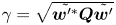 $\gamma =\sqrt {\tilde {\boldsymbol {w}'^{*}}\boldsymbol {Q} \tilde {\boldsymbol {w}'}}$.
Following Kerswell (Reference Kerswell2018), the algorithm for the update of  $\skew3\hat{\boldsymbol{f}}$ is based on steepest ascent
 \begin{equation} \,\hat{\boldsymbol{f}}_{{new}}=\,\hat{\boldsymbol{f}}+A \epsilon (\tilde{\boldsymbol{w}'} - 2\lambda \,\hat{\boldsymbol{f}}), \end{equation}
where the Lagrange parameter  $\lambda$ is chosen such that it constraints the forcing energy
 $\skew3\hat{\boldsymbol{f}}_{{new}}^{*}\boldsymbol {Q}\skew3\hat{\boldsymbol{f}}_{{new}}=A^{2}$, and
 $\epsilon$ governs the amplitude change between
 $\skew3\hat{\boldsymbol{f}}$ and
 $\skew3\hat{\boldsymbol{f}}_{{new}}$. The parameter
 $\epsilon$ may be chosen as
 $\epsilon =c/\gamma$, where
 $0 < c \leqslant 1$ to allow a solution for
 $\lambda$.
For  $c=1$,
 $\skew3\hat{\boldsymbol{f}}_{{new}}$ is parallel to the adjoint vector
 $\tilde {\boldsymbol {w}'}$ and the procedure is therefore similar to the power iteration method. Potentially, more efficient numerical methods can be implemented for the search direction (i.e. conjugate gradient instead of steepest ascent) and the update step length (line search methods for variable step size).
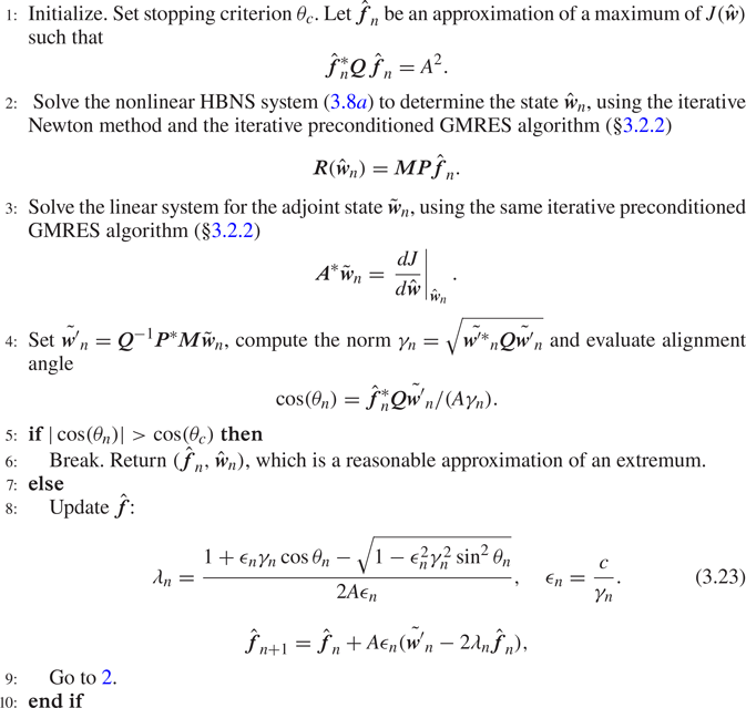
The explicit steps of the iterative procedure are detailed in algorithm 1. The parameter  $c$ can be fixed to 1 if the guess
 $\skew3\hat{\boldsymbol{f}}$ is close to the optimum. If not, large derivatives of the cost functional (i.e transition) can lead to large drifts of
 $\skew3\hat{\boldsymbol{f}}$, which may destabilise the Newton algorithm. In such a case, lower values of
 $c$ need to be imposed. In the present study, a good compromise was found with
 $c = 0.5$, for which most of the cases converged, without penalising too much the number of iterations for the Newton method to converge. In a few cases, we had to decrease the value of
 $c$ down to
 $c=0.2$. The stopping criterion was chosen so that the alignment
 $\theta$ is less than
 $\theta _c=1^{\circ }$.
Nonlinear optimisation using HBNS

4. HBNS: validation for controlled transition
In this section we validate the HBNS implementation described above against the DNS of controlled  $K$-type transition by Rist & Fasel (Reference Rist and Fasel1995). The volumetric forcing
 $\skew3\hat{\boldsymbol{f}}$ is set to zero and perturbations are triggered through
 $\hat {\boldsymbol {g}}$ which is chosen to represent wall-normal forcing by local time-dependent blowing and suction within a narrow strip at the wall. Thus, in accordance with Rist & Fasel (Reference Rist and Fasel1995), we impose
 $u=w=0$ and
 \begin{equation} v(x,z,t)= 5\times 10^{-3} \sin(\omega t) v_a(x) + 1.3\times 10^{-4} \cos(\beta z) v_s(x), \end{equation}
which represents a superposition of a 2-D spanwise uniform wave  $(0,\omega )$ of frequency
 $\omega =11\times 10^{-5}$ and a steady 3-D wave
 $(\beta ,0)$ of spanwise wavenumber
 $\beta =42.3\times 10^{-5}$. The specific profiles of the wall-normal velocity of the unsteady and steady waves, which are localised between
 $x_1$ and
 $x_2$ on the wall boundary, are given by
 \begin{gather} v_a(x)=\left\{ \begin{array}{ll} 0 , & x \leqslant x_1, \\ 15.1875 \xi^{5}-35.4375\xi^{4}+20.25\xi^{3} , & x_1 < x \leqslant x_m, \\ -v_a(2x_m-x) , & x_m < x \leqslant x_2, \\ 0 , & x_2 < x, \end{array}\right. \end{gather}
 \begin{gather}v_s(x)=\left\{ \begin{array}{ll} 0 , & x \leqslant x_1, \\ -3 \xi^{4}+4\xi^{3} , & x_1 < x \leqslant x_m, \\ v_s(2x_m-x) , & x_m < x \leqslant x_2, \\ 0 , & x_2 < x. \end{array}\right. \end{gather}
Here  $x_1=1.3438\times 10^{5}$ (
 $Re_{\delta ^{*}}^{1}=630$),
 $x_2=1.5532\times 10^{5}$ (
 $Re_{\delta ^{*}}^{2}=678$),
 $x_m=(x_1+x_2)/2$ and
 $\xi =({x-x_1})/({x_m-x_1})$. We have positioned the strip for exciting the disturbances exactly at the same location as in Rist & Fasel (Reference Rist and Fasel1995). The inlet and outlet positions of the domain (
 $Re_{\delta ^{*}}^{i} =298$ and
 $Re_{\delta ^{*}}^{o}=863$) are not identical to those of Rist & Fasel (Reference Rist and Fasel1995) (580 and 1375, respectively); yet, due to the convective amplification of disturbances in the boundary layer, these choices should not affect the comparison.
Due to the symmetry of the wall forcing, spanwise reflectional symmetry was assumed enforcing equations (3.14). The mean-flow harmonic  $\hat {\boldsymbol {w}}_{00}$ was initialised with the base-flow solution and the other harmonics were set to zero except the
 $(0,\omega )$ and
 $(\beta ,0)$ harmonics, which were initialised with the linearised responses. For
 $M=N=2$ (9 harmonics in total), the solution of the HBNS system converged after nine Newton iterations (residuals of the order of
 $10^{-10}$). The
 $M=N=3$ (16 harmonics) solution was obtained using as an initial guess the
 $M=N=2$ solution and converged after four iterations, whereas the
 $M=N=4$ (25 harmonics) solution was obtained from the
 $M=N=3$ one in four iterations. The associated computational cost in terms of memory, cores and walltime is given in table 3, appendix A.
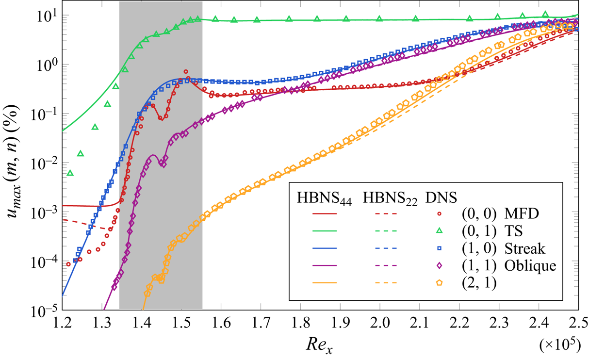
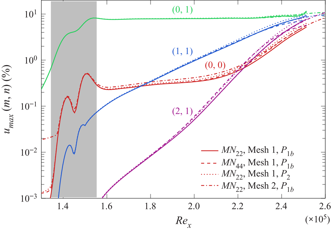
In figure 2 we compare the amplitude of the first few harmonics from the HBNS against the DNS results obtained by Rist & Fasel (Reference Rist and Fasel1995). A sensitivity analysis of the domain length and of the finite element discretisation is given in appendix A, along with the computational cost for the HBM method. For plotting the  $(0,0)$ harmonic component, we have subtracted the base-flow solution, which leads to the mean-flow deformation (MFD). The definition of the amplitudes of the different harmonics is described in appendix B. The wall-normal forcing excites initially planar TS waves
 $(0,\omega )$ and streamwise vortices/streaks
 $(\beta ,0)$ at a given frequency and spanwise wavelength. Oblique waves
 $(\beta ,\pm \omega )$ and higher harmonics are generated through nonlinear interactions. Similarly, the self-interaction of the modes when they reach sufficiently high amplitudes generates
 $(0,0)$ components that cause the departure of the mean-flow harmonic from the base-flow solution. Even with
 $M=N=2$, good agreement is obtained for the fundamental
 $(0,\omega )$ and
 $(\beta ,0)$ harmonics and for the oblique wave
 $(\beta ,\omega )$. As the perturbations grow in the streamwise direction, the
 $M=N=4$ results are in slightly better agreement with the DNS for the higher harmonic
 $(2\beta ,\omega )$.
Amplitudes of harmonics for  $K$-type controlled transition. Comparison between DNS (Rist & Fasel Reference Rist and Fasel1995) and harmonic-balanced Navier–Stokes retaining
 $M=N=2$ (
 $\textrm {HBNS}_{22}$) and
 $M=N=4$ (
 $\textrm {HBNS}_{44}$) harmonics in spanwise/frequency. The grey region denotes the streamwise extent of the wall blowing and suction region that triggers
 $K$-type transition. Note that to ease representation, we have plotted one fifth of the amplitude of harmonics
 $(0,\omega )$ and
 $(2\beta ,\omega )$.

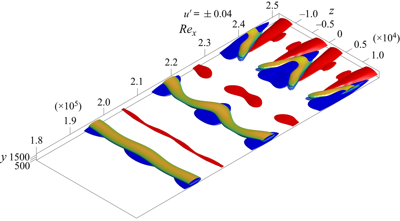
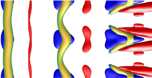
In figure 3 isosurfaces of streamwise velocity show low-speed velocity streaks (blue) developing in the streamwise direction. Furthermore, isosurfaces of the  $Q$-criterion, coloured based on the normal distance from the wall, show
 $\Lambda$-vortices sitting on the low-speed streaks. They are elongated and move away from the wall as they propagate downstream, in accordance with Rist & Fasel (Reference Rist and Fasel1995). The more localised the
 $\Lambda$-structure, the larger the number of harmonics required in the
 $z$-direction to describe it. It is seen that with
 $M=4$, we clearly capture these structures.
 $K$-type controlled transition with
 $\textrm {HBNS}_{{44}}$. Isosurfaces of perturbation velocity
 $u'=\pm 0.04$ (red: high speed, blue: low speed) and of the second invariant of the velocity gradient tensor,
 $Q$, coloured by the vertical distance from the wall (
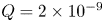 $Q = 2\times 10^{-9}$).

It is evident that linear approaches would fail to capture the observed transition dynamics, including mean-flow deformation and saturation of the amplitude of the harmonics. Potentially a quasi-linear approach could be used to calculate the mean-flow deformation but, in general, the nonlinear energy transfer between the forced modes is not captured. And consequently, also the resulting mean-flow deformation arising from the triadic nonlinearly excited modes. In the specific case of  $K$-type examined by Rist & Fasel (Reference Rist and Fasel1995), this is evident by observing that energy is transferred to the oblique wave due to the nonlinear interaction of the streak and planar 2-D wave components.
The HBNS framework captures all the above key dynamical characteristics of transition (mean-flow deformation, saturation, nonlinear energy transfer among harmonics) by keeping the minimum number of harmonics and consequently the minimum number of balanced nonlinear interactions.
The question that arises is how many modes and consequently nonlinear interactions are needed for a qualitative and quantitative description of the flow? As expected, the higher the amplitude of the perturbations, the more harmonics are needed in the HBNS representation: the upstream (respectively downstream) part of the flow, which is characterised by small (respectively large) perturbations, requires a low (respectively high) truncation order. The number of required harmonics, therefore, depends on the forcing amplitude and the extent of the domain in the downstream direction, which sets the maximum amplitude of the perturbation.
5. Linear input/output (resolvent) analysis
Before performing nonlinear optimisation, we briefly recall here results obtained by Monokrousos et al. (Reference Monokrousos, Åkervik, Brandt and Henningson2010), Brandt et al. (Reference Brandt, Sipp, Pralits and Marquet2011) concerning linear optimal forcing in the frequency domain that aim at maximising energetic gains (resolvent analysis). Such results are important to understand and analyse the forthcoming nonlinear optimisations. For this, we consider a generic volumetric forcing and no-slip boundary conditions on the wall. For a given forcing  $\skew3\hat{\boldsymbol{f}}_{mn}$ and response
 $\hat {\boldsymbol {w}}_{mn}$ harmonic, the cost function for the linear optimisation is the input/output kinetic energy gain over the whole domain
 \begin{equation} J^{{lin}}_{mn} = \frac{\hat{\boldsymbol{w}}^{*}_{mn}\boldsymbol{Q}'_{mn}\hat{\boldsymbol{w}}_{mn}}{\,\hat{\boldsymbol{f}}^{*}_{mn}\boldsymbol{Q}_{mn}\,\hat{\boldsymbol{f}}_{mn}}, \end{equation}
where  $\boldsymbol {Q}'_{mn}$ eliminates the pressure component of the state vector
 $\boldsymbol {w}=[u,v,w,p]$ for the calculation of the kinetic energy solely on the velocity components,
 \begin{equation} \boldsymbol{Q}'_{mn}=\left( \begin{array}{cc} \boldsymbol{Q}_{mn} & 0 \\ 0 & 0 \end{array} \right), \end{equation}
and  $\boldsymbol {Q}_{mn}$ was defined in (3.18).
Although we could have used the nonlinear HBNS code with a small forcing amplitude  $A$, such that nonlinear effects are negligible, we used a linearised version of the code implementing the linear relationship between
 $\skew3\hat{\boldsymbol{f}}_{mn}$ and
 $\hat {\boldsymbol {w}}_{mn}.$ Such a linear optimisation problem is efficiently solved by iterative methods (Sipp & Marquet Reference Sipp and Marquet2013). The mesh extends here from
 $x_i=0.30 \times 10^{5}$ (
 $Re_{\delta ^{*}}^{i}=298$) to
 $x_o=3.60 \times 10^{5}$ (
 $Re_{\delta ^{*}}^{o}=1032$). It comprises 116 806 triangles, yielding 586 178 degrees of freedom per harmonic. The same mesh will be used in the next section dealing with nonlinear optimisation (§ 6).
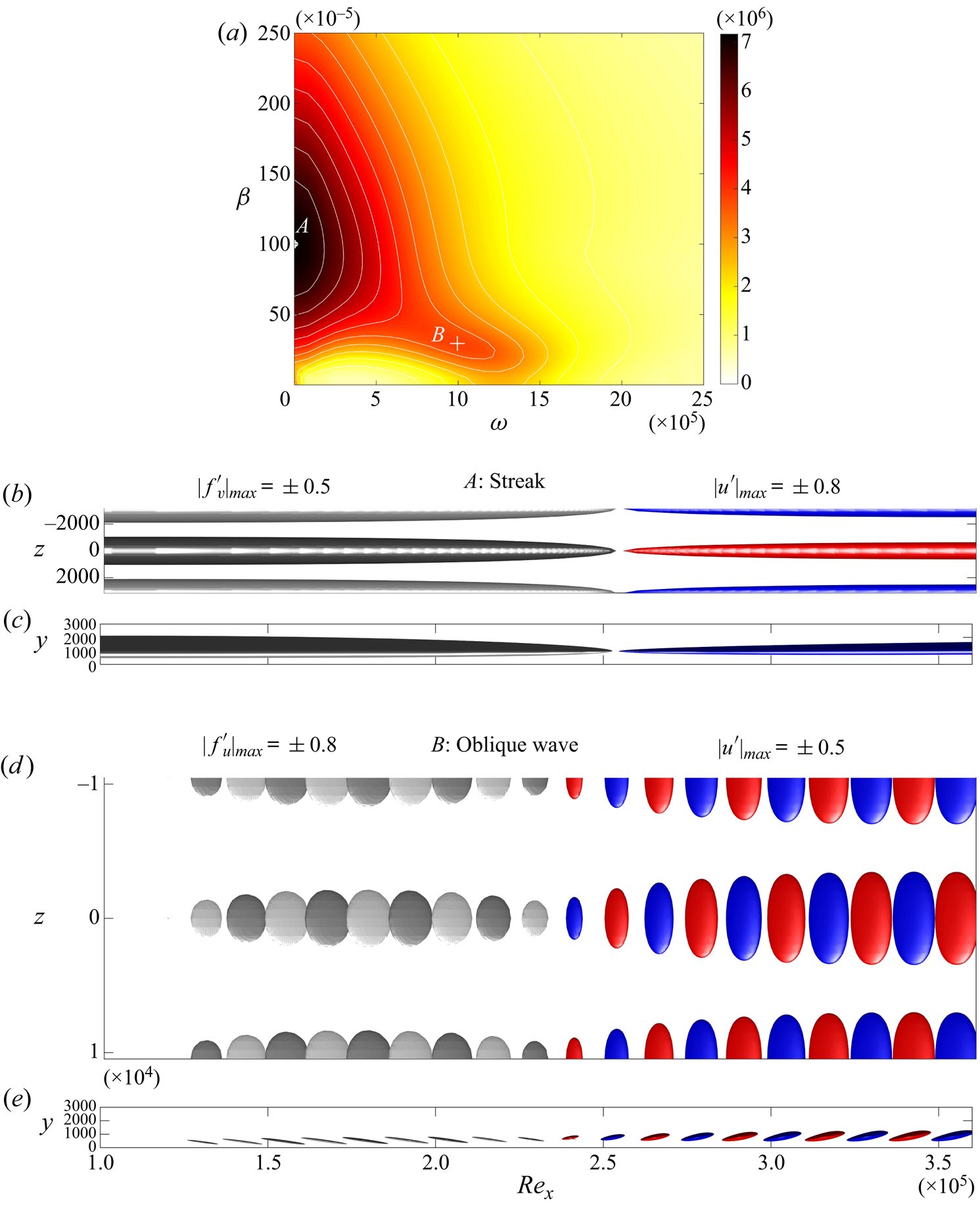
The linear optimal amplitude gain ( $\sigma =\sqrt {J^{{lin}}_{mn}}$) is shown in figure 4, as a function of frequency
 $\omega$ and spanwise wavenumber
 $\beta$. Two local maxima are observed, in agreement with Monokrousos et al. (Reference Monokrousos, Åkervik, Brandt and Henningson2010). The forcing and response mode shapes of the two linear optimal mechanisms are shown in the same figure.
Linear input/output (resolvent) analysis. Optimal gain (a). The two local maxima correspond to the amplification of streaks ( $A$ at
 $(\beta ,\omega ) =(100,0)\times 10^{-5}$) and oblique waves (
 $B$ at
 $(\beta ,\omega ) =(30,10)\times 10^{-5}$). Optimal forcing (left; light grey: positive, dark grey: negative) and optimal response (right; red: positive, blue negative) for streaks and obliques waves. Top and side views are shown. The
 $x$-axis has been scaled by a factor of 4.

The first local maximum at  $(\beta ,\omega ) =(100,0)\times 10^{-5}$, point
 $A$, is associated with the non-modal lift-up mechanism. The optimal forcing corresponds to steady streamwise rolls (
 $v$,
 $w$ components; for the optimal forcing, the
 $v$ component is shown), and the optimal response to streamwise streaks located further downstream (
 $u$ component).
The second local maximum at  $(\beta ,\omega ) =(30,10)\times 10^{-5}$, point
 $B$, corresponds to the amplification of oblique TS waves. The planar TS waves are not the most amplified ones due to the cooperative non-modal amplification through the Orr and lift-up mechanisms. It is clearly noticed that the optimal forcing is tilted upstream, against the mean shear so that the response takes advantage of the algebraic amplification through the Orr mechanism.
6. Nonlinear input/output analysis
To uncover the optimal nonlinear mechanisms that promote transition, the nonlinear interactions of the modes and their impact on the mean flow is now incorporated in the analysis through the optimisation approach developed in § 3.3.
We choose as cost function the (squared) shear stress of the mean-flow deviation, integrated over the wall. With the notation introduced above, this is
 \begin{equation} J(\hat{\boldsymbol{w}})=J(\hat{\boldsymbol{w}}_{00})=(\hat{\boldsymbol{w}}_{00}-\boldsymbol{w}_b)^{*}\boldsymbol{C}^{*}\boldsymbol{C}(\hat{\boldsymbol{w}}_{00}-\boldsymbol{w}_b), \end{equation}
with  $\boldsymbol {C}\boldsymbol {w} = \int _{y=0} ({\partial u}/{\partial y} )\,\textrm {d}x$ and
 $\boldsymbol {w}_b$ is the base flow. For this choice of cost function, we have
 \begin{equation} \frac{\textrm{d}J}{\textrm{d}\hat{\boldsymbol{w}}_{00}}=2\boldsymbol{C}^{*}\boldsymbol{C}(\hat{\boldsymbol{w}}_{00}-\boldsymbol{w}_b) \end{equation}
and  $0$ for the other harmonics. This cost function can be directly linked to the drag change exerted on the plate,
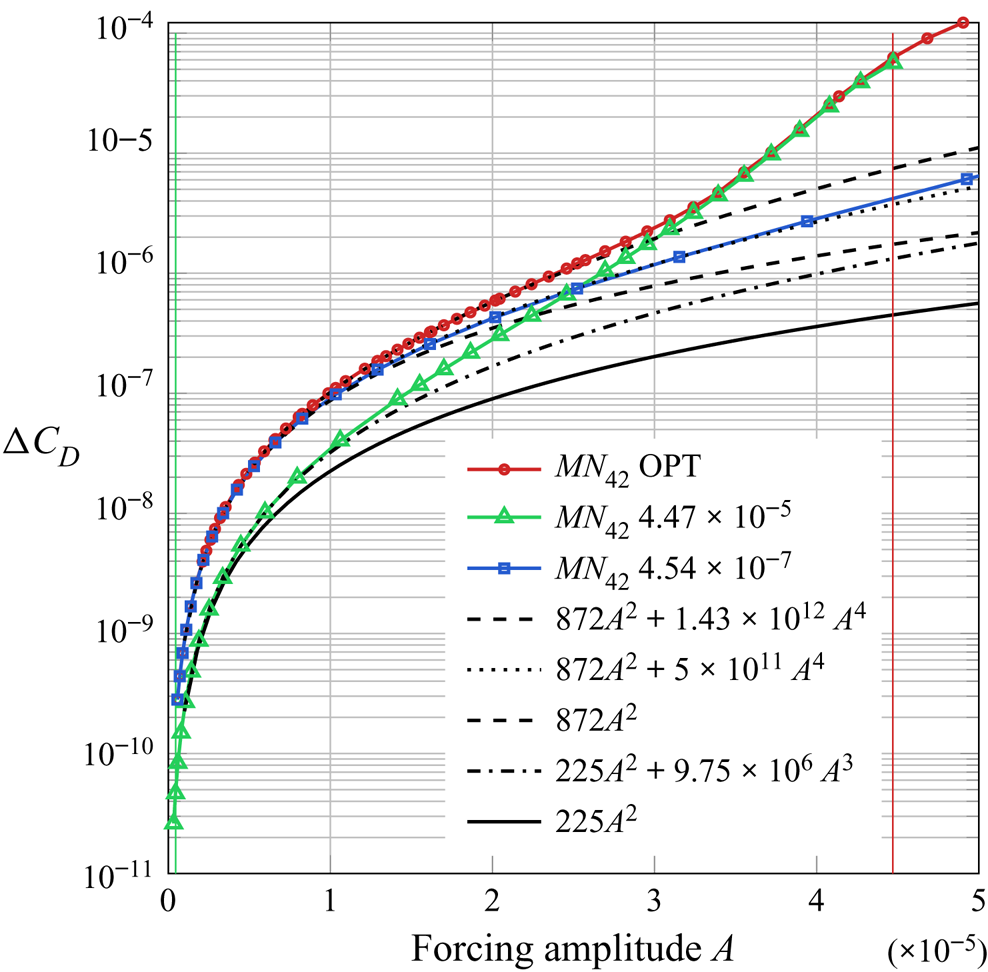
 \begin{equation} {\rm \Delta} C_D = \frac{\nu J^{0.5}}{\frac{1}{2} U_\infty^{2} L_p}, \end{equation}
where  $L_p=x_o$ is the plate length. In other words, by maximizing the specific cost function
 $J$, we maximize the drag on the plate.
The entries of matrix  $\boldsymbol {P}$ allow selection of the forced equations and of a subset of forced harmonics. As in the linear case, we will restrict the forcing to the momentum equations and exclude mass sources. In order to preserve the mean-flow harmonic
 $\hat {\boldsymbol {w}}_{00}$ from direct modifications induced by steady forcing terms, we set
 $\skew3\hat{\boldsymbol{f}}_{00}=0$ and exclude this mode from the optimisation process. Thus, we focus on environmental perturbations that trigger transition which are, in principle, characterised by zero mean in
 $z$ and
 $t$, and they do not introduce directly a mean-flow deformation. Yet, we allow steady forcing in
 $z$, i.e. rolls with
 $\textrm {e}^{\textrm {i}\beta z}$ shape, that trigger mean-flow deformations in
 $z$.
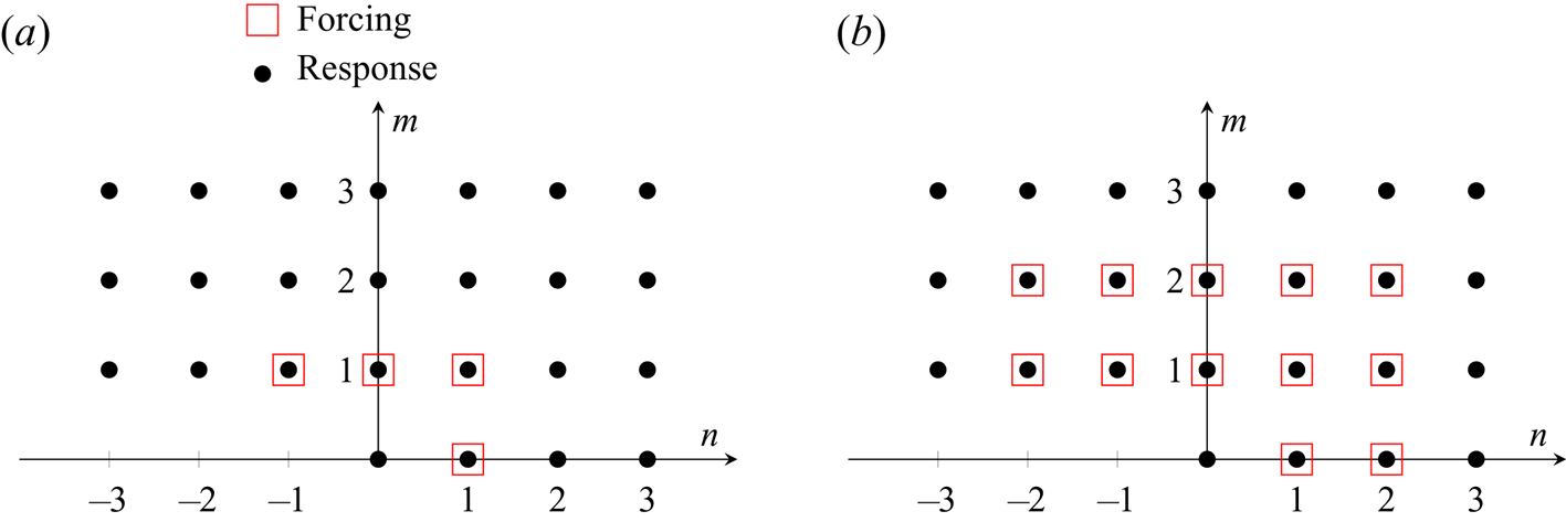
Two types of forcing are then considered, which we refer to as fundamental and superharmonic cases, as depicted in figure 5. For the first case, forcing is restricted to components  $(m,n)=(\beta ,\pm \omega )$,
 $(\beta ,0)$,
 $(0,\pm \omega )$; we call this fundamental since forcing is allowed only at the primary forcing frequency and spanwise wavenumber. Each of these forcing components can potentially lead to the amplification of a pair of unsteady oblique waves, steady streamwise streaks or vortices, and planar waves, respectively. For the superharmonic forcing case, we allow also the second forcing harmonics to be optimised,
 $|m| \leqslant 2$ and
 $|n| \leqslant 2$, except
 $m=n=0$. This allows forcings comprising of fundamental superharmonic components. For example, forcing
 $\skew3\hat{\boldsymbol{f}}_{02}$ is at twice the frequency of forcing
 $\skew3\hat{\boldsymbol{f}}_{11}$. If the perturbation satisfies reflectional symmetry in
 $z$, all forcing and response harmonics
 $n<0$ are directly linked to those satisfying
 $n > 0$. The range of fundamental forcing frequencies and spanwise wavenumbers for the nonlinear optimisation were chosen such that the linear optimal mechanisms corresponding to streaks and oblique waves, see linear
 $\beta -\omega$ gain map in figure 4, are investigated in the nonlinear framework. We note that in both cases, we solve 132 separate optimisation cases over a wide range of the fundamental forcing frequency,
 $\omega$ and
 $\beta$. Specifically,
 $\beta =[4.1,8.3,16.6:16.6:167] \times 10^{-5}$ and
 $\omega =[0.83,1.67:1.67:16.67]\times 10^{-5}$.
Fundamental (a) and superharmonic (b) cases. The nonlinear optimisation is restricted to forcing components  $1\beta ,\pm 1\omega$, or
 $1\beta ,2\beta ,\pm 1\omega ,\pm 2\omega$, and their oblique combinations, respectively. Other forcing and response harmonics in the
 $(m,n)$ plane may be deduced from the real-value constraint, e.g.
 $\hat {\boldsymbol {w}}_{-m-n}=\overline {\hat {\boldsymbol {w}}_{mn}}$. In case of reflectional symmetry in
 $z$, the
 $-n \omega$ components are linked to the
 $+n\omega$ ones.

As an initial guess to the nonlinear optimisation algorithm, we use the base-flow solution for the mean-flow harmonic  $\hat {\boldsymbol {w}}_{00}$ and the linear optimal forcing and response components that maximize the kinetic energy (see § 5) for the perturbation (all unforced harmonics are set to zero). The amplitude of each harmonic forcing
 $\skew3\hat{\boldsymbol{f}}$ is normalized based on the linear gain
 \begin{equation} \,\hat{\boldsymbol{f}}_{mn}^{{init}}=\zeta \frac{\,\hat{\boldsymbol{f}}_{mn}^{{lin}}}{\sqrt{\lambda_{mn}}}, \end{equation}
where  $\skew3\hat{\boldsymbol{f}}_{mn}^{{lin}}$ is a unit-norm (based on
 $\boldsymbol {Q}_{mn}$) linear optimal forcing associated to the linear optimal gain
 $\lambda _{mn}$ and
 $\zeta$ a constant adjusted so that
 $\skew3\hat{\boldsymbol{f}}^{*}\boldsymbol {Q} \skew3\hat{\boldsymbol{f}}=A^{2}$. Such a choice allows the initial condition
 $\hat {\boldsymbol {w}}^{{lin}}$ to correspond to a mix of optimal responses of equal amplitude. The nonlinear optimisation framework then adjusts their amplitude, their spatial shape and fills in the response modes arising from the nonlinear interactions.
Regarding the initial amplitude  $A$, we choose a low value, for which it is easy to converge to the nonlinear solution due to its proximity to the linear regime. Then, we gradually increase
 $A$ and follow the solution. The optimal solution is defined up to a phase due to the periodicity in time (for example,
 $t=0$ can correspond to an arbitrarily defined phase). Without imposing a
 $z$-symmetry, the same is true for the
 $z$-direction, meaning the
 $z=0$ location has an arbitrarily defined phase. Only in the symmetric case, the phase in
 $z$ is fixed. For high amplitudes, multiple solutions may exist. For that reason, we have added random noise to test the robustness of our solutions. After a high threshold, we indeed identified a non-symmetric branch of solutions in addition to the low amplitude symmetric one, which are discussed in the following sections.
6.1. Identification of optimal transition mechanisms: $z$-symmetric case with $A=7.07\times 10^{-5}$ and $M=N=2$



We first consider a case with imposed spanwise symmetry on the forcing and response and  $M=N=2$. For small enough amplitude
 $A$, we expect that the forcing and perturbation should exhibit the
 $z$-reflectional symmetry of the configuration. The small number of resulting modes allows for more expensive parametric studies over
 $\omega$ and
 $\beta$, but, strictly speaking, the results are converged for sufficiently small
 $A$ so that higher-order harmonics may be neglected. We look for an amplitude
 $A$ that is sufficiently large so that nonlinear interactions and energy transfers are effective but also sufficiently small to ensure that truncation errors are negligible for
 $M=N=2$. We found the value
 $A=7.07\times 10^{-5}$ to be a good compromise. In a subsequent section we examine convergence by increasing
 $A$ and the retained number of harmonics
 $M$ and
 $N$, and verify a posteriori that the present results are reasonably well converged.
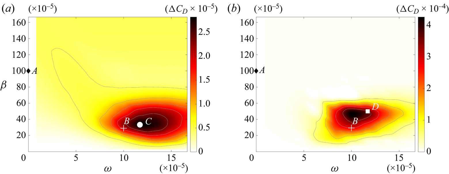
The cost function (expressed as mean drag perturbation via (6.3)) is shown in figure 6 for both the fundamental- and superharmonic-type forcings. For the fundamental case, maximum drag increase is observed at  $(\beta ,\omega ) =(33.4,11.7)\times 10^{-5}$, whereas for the superharmonic case, the maximum occurs at the same frequency but a slightly higher wavenumber,
 $(\beta ,\omega ) =(50,11.7)\times 10^{-5}$. For the superharmonic case, the drag increase is approximately 14 times higher compared with the fundamental forcing. In both cases, the overall optimal frequency/wavenumber pairs are close to the point marked
 $B$ on the linear amplification plot (figure 4), which represents the local maximum in linear amplification of oblique waves. While those waves are linearly less amplified than streaks (point
 $A$), they are nonlinearly superior. As will be shown in detail below, the nonlinear fundamental mechanism
 $C$ and superharmonic mechanism
 $D$ initially harness oblique wave amplification, and eventually lead, through nonlinearity, to redistribution of energy near
 $A$ and a strong response related to the lift-up mechanisms producing streaks.
Optimal drag change from nonlinear input/output analysis with (a) fundamental and (b) superharmonic forcing,  $M=N=2$ and
 $A=7.07\times 10^{-5}$. In both cases, we solve separate optimisation cases over a wide range of the fundamental forcing frequency,
 $\omega$ and
 $\beta$. Fundamental maximum at point
 $C$:
 ${\rm \Delta} C_{D,max}=2.8\times 10^{-5}$ at
 $(\beta ,\omega ) =(33.4,11.7)\times 10^{-5}$. Superharmonic maximum at point
 $D$:
 ${\rm \Delta} C_{D,max}=41.6\times 10^{-5}$ at
 $(\beta ,\omega ) =(50,11.7)\times 10^{-5}$. Both maxima are close to the optimal linear amplification of the oblique waves (point
 $B$).

6.1.1. Symmetric fundamental forcing
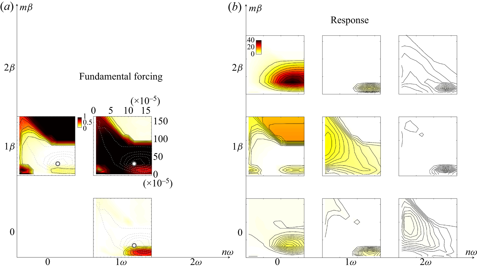
Focusing on the fundamental case first (figure 5a) with  $z$-reflectional symmetry, we now delve into the optimal forcing and response in greater detail. To simplify the discussion, we define in appendix B, a scalar amplitude
 $A(m,n)$ of each forcing/response mode, which represents an integral over the spatial domain. These amplitudes are shown in figure 7. Note that upon summation of the forcing modes, this yields the overall forcing amplitude (here
 $A=7.07\times 10^{-5}$), and all amplitudes in the plot are normalized by this value. Based on the dominant regions of the forcing and response amplitudes on the
 $\beta$–
 $\omega$ planes in figure 7, three distinct mechanisms can be identified.
(i) Oblique waves. The maximal drag increase over the entire
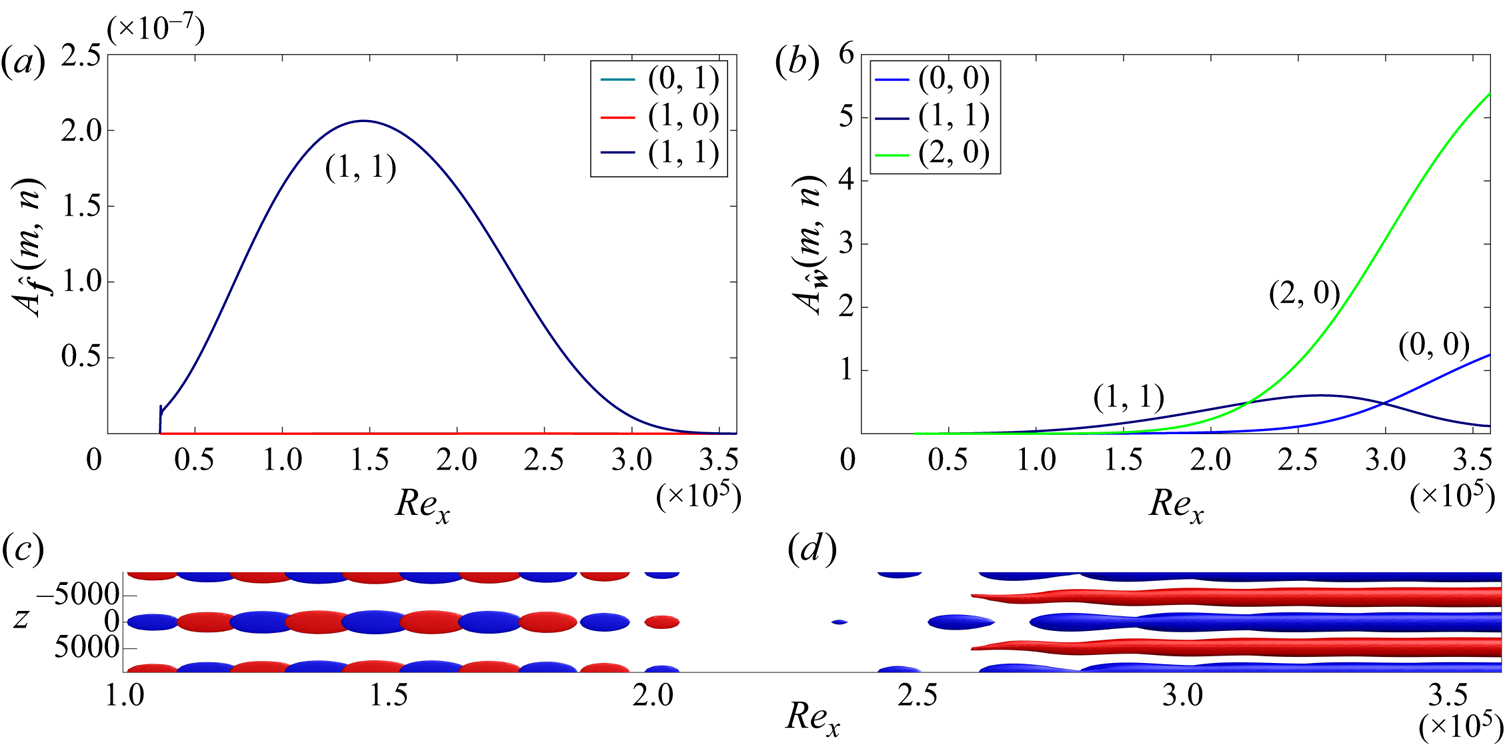
$\beta$–$\omega$ plane examined here occurs for $(\beta ,\omega )=(33.3,11.7)\times 10^{-5}$, and only involves significant forcing of the oblique wave component $(\beta ,\pm \omega )$. In the response, there is some amplification to the response component $(\beta ,\pm \omega )$, as expected in a linear framework, but the $(2\beta ,0)$ component, which arises from nonlinear interactions between $(\beta ,\omega )$ and $(\beta ,-\omega )$ components, is highly amplified. The mean-flow modification is clearly associated with the amplification of $(2\beta ,0)$ streaks via oblique forcing. These observations confirm oblique transition as optimal in terms of transition thresholds among all the fundamental spanwise-symmetric mechanisms, as shown previously for plane Couette (Duguet, Brandt & Larsson Reference Duguet, Brandt and Larsson2010) and channel flow (Reddy et al. Reference Reddy, Schmid, Baggett and Henningson1998).(ii) Streamwise vortices. For high spanwise wavenumbers,
$\beta >100\times 10^{-5}$, the optimal forcing is a streamwise vortex $(m,n)=(\beta ,0)$. For these frequencies, the linear amplification of oblique waves is weak and, thus, the generated streaks through nonlinearity would also be weak. Consequently, for high enough frequencies and wavenumbers, i.e. those that are far from the linear optimal of the oblique waves, the optimal forcing mechanism is the direct amplification of streaks through the lift-up mechanism.(iii) K-type mechanism. Finally, at
$(\beta ,\omega )=(16,15)\times 10^{-5}$, the optimal forcing is a combination of all three components. Main forcing component is a planar 2-D wave $(0,\omega )$ followed by a pair of 3-D oblique waves $(\beta ,\pm \omega )$ at the same frequency. This mechanism is similar to the Klebanov one, describing fundamental $K$-type transition.





Nonlinear optimisation for fundamental  $z$-symmetric forcing with
 $M=N=2$. Amplitudes of optimal forcing (a) and response (b) for each individual harmonic component
 $(m,n)$, as depicted in figure 5(a). Values have been normalised with the total forcing amplitude
 $A=7.07\times 10^{-5}$. The circle marks the frequency/wavenumber that maximum drag increase is observed. Also, isolines of the cost function (dashed lines) have been added on the forcing components.

Since the oblique waves are the most dangerous mechanism in terms of drag increase, we examine the structure of the forcing and response fields in greater detail in figure 8. Initially,  $(\beta ,\pm \omega )$ oblique waves (only oblique waves with positive wavenumber and frequency are shown due to
 $z$-symmetry) are amplified due to linear instability and reach maximum amplitude at
 $Re_x\approx 250\,000$ before they start decaying. The optimal forcing is located further upstream and exploits the Orr mechanism for the amplification of the oblique waves, similarly to the optimal linear mechanism. Both the linear (§ 5) and nonlinear (shown in this section) optimal oblique forcings reach their maximum value around
 $Re_x\approx 150\,000$, which is near branch I of the neutral amplification curve based on modal stability analysis (see Sipp & Marquet (Reference Sipp and Marquet2013) regarding the link between local modal stability and linear resolvent). The quadratic nonlinearity redistributes the energy of the oblique waves into the
 $(2\beta ,0)$ mode in the form of streamwise vortices with streamwise vorticity
 $\omega _x$ (
 $v,w$ components with
 $(2\beta ,0)$). In turn, the streamwise vortices lead to the growth of the streaks (
 $u$ component with
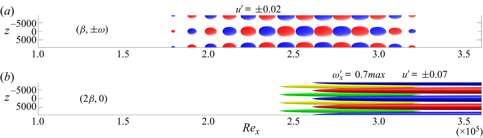
 $(2\beta ,0)$) through the linear lift-up mechanism. The spatial shape of each harmonic response component mentioned above is shown in figure 9, demonstrating the transition sequence from oblique waves to streamwise vortices and streaks. These observations are in agreement with previous studies on oblique transition (Schmid & Henningson Reference Schmid and Henningson1992; Berlin, Lundbladh & Henningson Reference Berlin, Lundbladh and Henningson1994). The sequential temporal unfolding of the Orr, oblique and lift-up phases has been observed during the minimal seed calculations in the time domain (Pringle et al. Reference Pringle, Willis and Kerswell2012; Duguet et al. Reference Duguet, Monokrousos, Brandt and Henningson2013), in analogy to the spatial unfolding of the above mechanisms in the streamwise direction during the present approach.
Optimal oblique fundamental case with  $M=N=2$ at
 $(\beta ,\omega )=(33.3,11.7)\times 10^{-5}$ for
 $A=7.07\times 10^{-5}$. This forcing results to the maximum amplification of shear stress for fundamental forcing over all forcing frequencies and wavenumbers (point
 $C$ in figure 6a). Isosurfaces of streamwise perturbations
 $f'_u= \pm 8.3\times 10^{-9}$ (c) and
 $u'= \pm 0.07$ (d), blue negative isovalue and red positive one. One fundamental wavelength is shown in
 $z$.

Harmonic response components for the optimal oblique fundamental case shown in figure 8. The response is dominated by the growth of  $(\beta ,\pm \omega )$ oblique waves (
 $u'$ shown), followed by the nonlinear generation of
 $(2\beta ,0)$ streamwise vortices (
 $\omega '_x$ shown) and the linear growth of streaks (
 $u'$ shown).

The link between the nonlinear gain map and that obtained from linear analysis is evident now: the most dangerous nonlinear forcing exploits both linear amplification mechanisms, specifically 3D unsteady oblique waves and 3-D steady rolls–streaks, through the redistribution of energy from the first linear mechanism to the second linear mechanism via nonlinearity. The fundamental frequency and spanwise wavenumber,  $(\beta ,\omega )=(33.3,11.7)\times 10^{-5}$, is very close to the linearly optimal oblique ones,
 $(\beta ,\omega )=(30,10)\times 10^{-5}$, and then nonlinearly generated steady vortices are formed at twice the spanwise wavenumber
 $(\beta ,\omega )=(66.6,0)\times 10^{-5}$. The latter part does not coincide with the maximum linearly amplified lift-up wavenumber,
 $(\beta ,\omega )=(100,0)\times 10^{-5}$, but it is close enough to take advantage of this mechanism in an optimal synergistic way.
6.1.2. Symmetric superharmonic forcing
Here, the forcing is expanded to consider both the fundamental and its first harmonic in both frequency and spanwise wavenumber, see figure 5(b). Thus, forcing is allowed in eight forcing components arising from all the combinations of fundamental and first harmonic components. We retain for now  $M=N=2$ and
 $A=7.07\times 10^{-5}$, and recall (figure 6b) that maximum amplification of shear stress is observed for forcing at
 $(\beta ,\omega )=(50,11.7)\times 10^{-5}$.
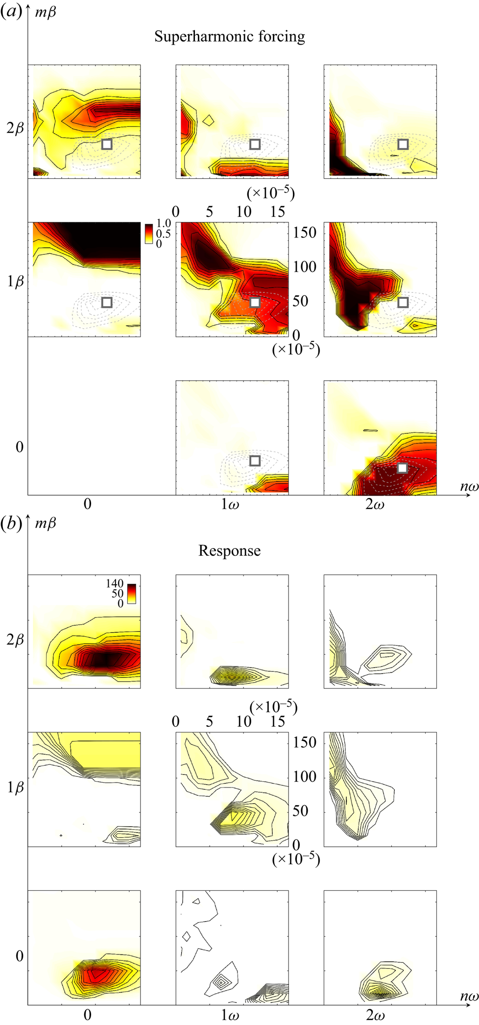
The optimum in the  $(\beta ,\omega )$ plane for the superharmonic case is close to the one found for the fundamental case where the oblique waves were the optimal forcing mechanism. However, now the planar waves at twice the frequency of the oblique waves share similar amplitude to the oblique waves. As can be observed in figure 10, only two major forcing components exist at the optimal
 $(\beta ,\omega )$ pair. The optimal forcing corresponds to a three-dimensional oblique wave
 $(\beta ,\omega )$ and a superharmonic two-dimensional wave at twice the frequency,
 $(0,2\omega )$. The optimal superharmonic forcing is in agreement with the typical scenario for
 $H$-type transition triggered by a pair of oblique waves and a TS wave at twice the frequency. In the literature describing
 $H$-type transition, typically the TS is called the fundamental wave and the oblique the subharmonic, but our description is equivalent.
Nonlinear optimisation for superharmonic  $z$-symmetric forcing
 $M=N=2$. Amplitudes of optimal forcing (a) and response (b) for each individual harmonic component
 $(m,n)$, as depicted in figure 5(b). Values are normalised with the total forcing amplitude
 $A=7.07\times 10^{-5}$. The square marks the frequency/wavenumber that maximum drag increase is observed.

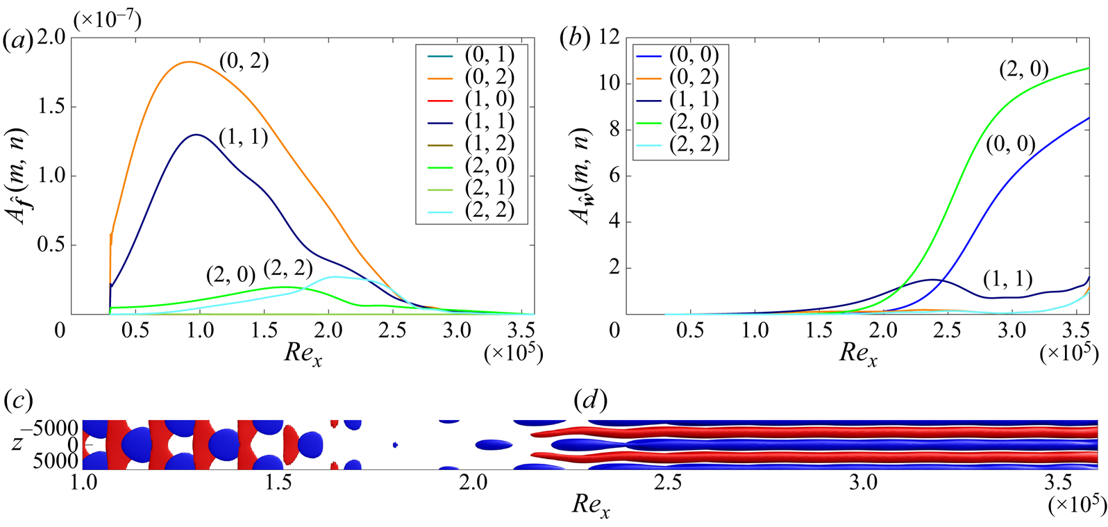
The streamwise evolution of each forcing and response harmonic for the optimal superharmonic case is shown in figure 11. The forcing is dominated by the superharmonic two-dimensional TS wave at twice the fundamental frequency,  $(0,2\omega )$, and the three-dimensional oblique waves,
 $(\beta ,\pm \omega )$. Since spanwise reflectional symmetry has been enforced, the amplitudes of the
 $(\beta ,+\omega )$ and
 $(\beta ,-\omega )$ oblique waves are equal and only one of those is shown. Despite the differences in the forcing components when compared with the fundamental case where only the oblique waves are present, the amplitude response is qualitatively similar and dominated by streaks. However, the nonlinearly generated streaks have almost twice as high amplitude when compared with the fundamental case, due to the efficient amplification of the parent oblique waves through the resonant interaction with the planar 2-D waves (see figure 12). The subsequent stages are similar to the ones of the fundamental case where streamwise vortices are generated from the nonlinear interactions between
 $(\beta ,\omega )$ and
 $(\beta ,-\omega )$ components, which in turn produce streaks. Finally, towards the end of the domain, low- and high-speed streaks start to undergo streamwise oscillations. These oscillations are stronger than in the fundamental oblique case (compare with figure 8), since for a given amplitude, the resonant
 $H$-type forcing leads to higher streak amplification through the stages described above.
Optimal  $H$-type superharmonic case
 $M=N=2$ at
 $(\beta ,\omega )=(50,11.7)\times 10^{-5}$ for
 $A=7.07\times 10^{-5}$. This forcing results to the maximum amplification of shear stress for superharmonic forcing over all forcing frequencies and wavenumbers (point
 $D$ in figure 6b). Isosurface of
 $f'_u= \pm 8.3\times 10^{-9}$ (c) and
 $u'= \pm 0.07$ (d), blue negative isovalue and red positive one. One fundamental wavelength is shown in
 $z$.

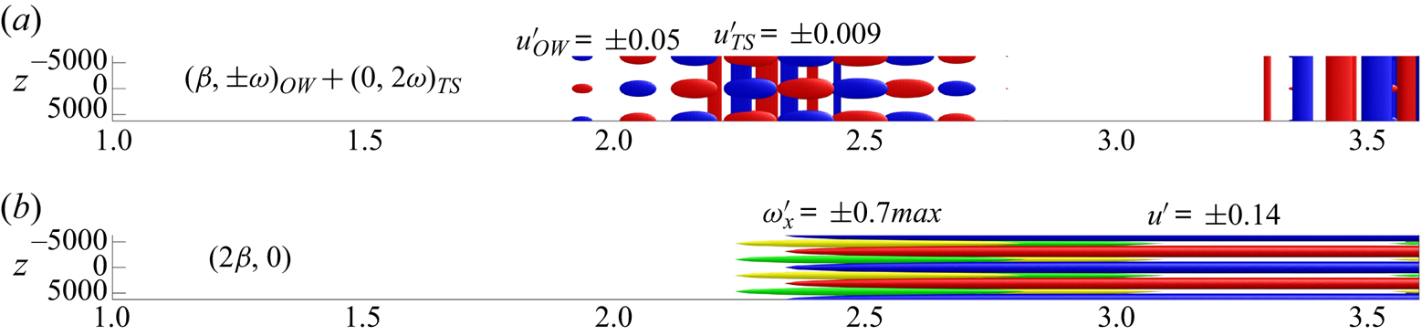
Harmonic response components for the optimal superharmonic case shown in figure 11. The response is dominated by the growth of  $(\beta ,\pm \omega )_{OW}$ oblique waves (OW) and planar waves
 $(0,2\pm \omega )_{TS}$ at twice the fundamental frequency (
 $u'$ overlaid for OW and TS) characteristic of
 $H$-type resonance. The oblique waves generate nonlinearly
 $(2\beta ,0)$ streamwise vortices (
 $\omega '_x$ shown) which promote the linear growth of streaks (
 $u'$ shown). Also, initial stages of streak instability are observed near the domain outlet.

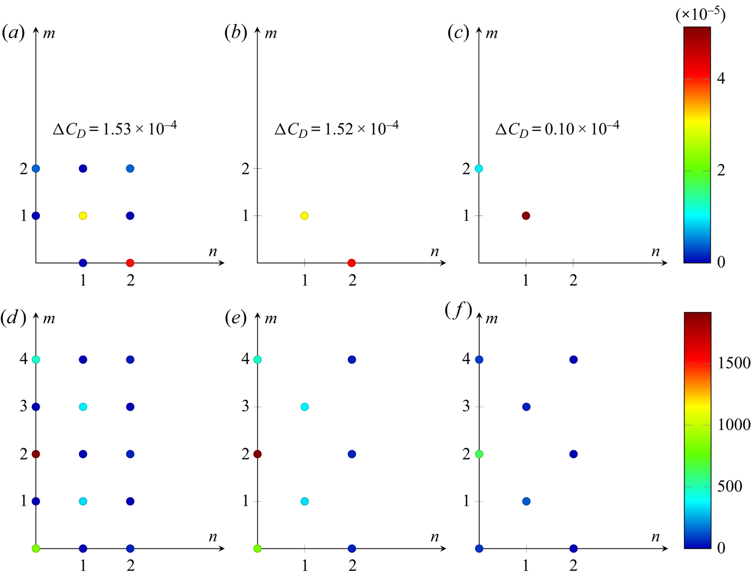
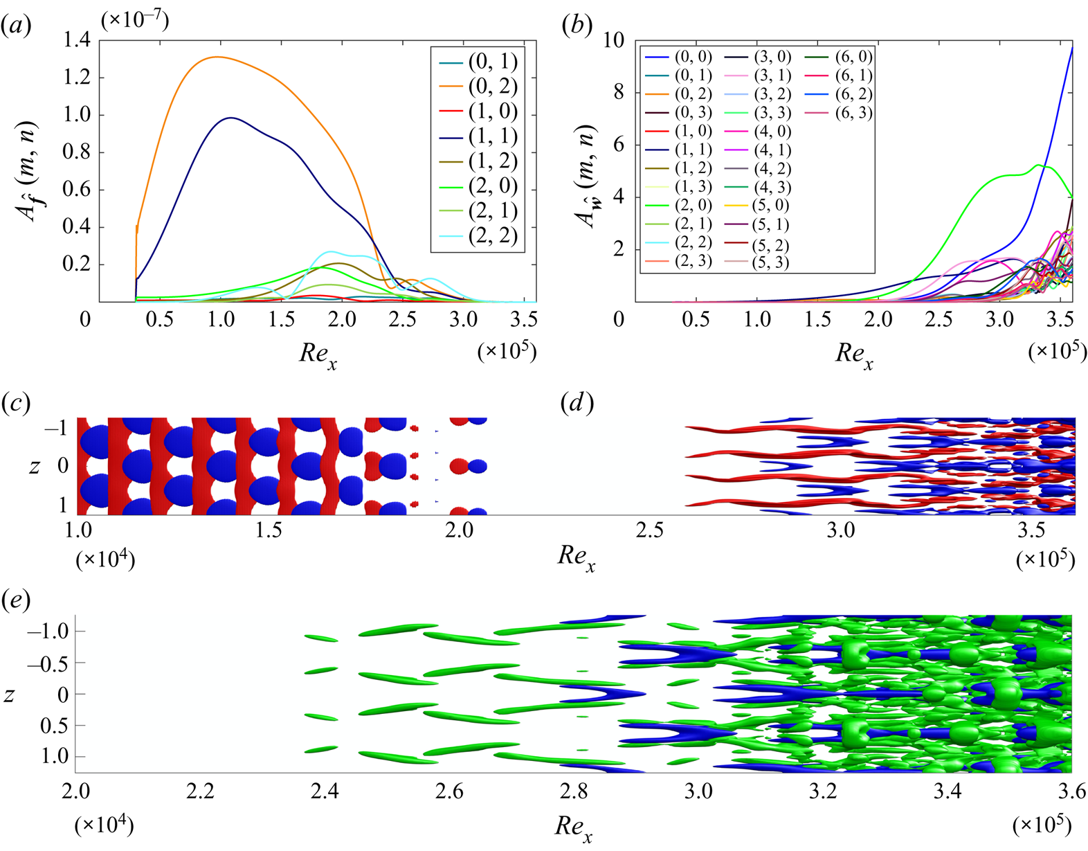
For the optimal superharmonic forcing (oblique and planar waves), low levels of energy are observed in two other forcing components, the  $(2\beta ,0)$ and
 $(2\beta ,2\omega )$ components. In figure 13 we analyse their importance by plotting the total amplitude of each forcing and response harmonic. Also, to ensure converged results, we have increased the number of response harmonics and lowered the forcing amplitude. The left column shows the superharmonic optimised forcing and response amplitude for each harmonic, when forcing is allowed in all eight forcing components as above. The
 $(0,2\omega )$ planar and
 $(\beta ,\omega )$ oblique waves are the dominant forcing components, and the
 $(2\beta ,0)$ and
 $(4\beta ,0)$ streaky structures, the
 $(\beta ,\omega )$ and
 $(3\beta ,\omega )$ oblique waves and the
 $(0,0)$ MFD in the response. The second column corresponds to an optimisation restricted solely to the
 $(0,2\omega )$ and
 $(\beta ,\omega )$ harmonics: it is seen that it reproduces closely the more complex optimisation of the left column (the reached
 ${\rm \Delta} C_D$ is nearly the same). In contrast (right column), it is seen that if the
 $(0,2\omega )$ planar wave is replaced by the
 $(2\beta ,0)$ streaky component in the forcing (this also corresponds to a superharmonic forcing but in spanwise wavenumber), then the optimal response only achieves weak drag increase, in agreement with those shown for the fundamental optimisation at similar amplitudes. This validates that it is the interplay between the
 $(0,2\omega )$ planar and the
 $(\beta ,\omega )$ oblique harmonic that accounts for the strong amplification observed in
 $H$-type transition.
Optimal forcing (a–c) and response (d–f) amplitudes for superharmonic cases  $M=4$,
 $N=2$ at
 $(\beta ,\omega )=(50,11.7)\times 10^{-5}$ for
 $A=5.13\times 10^{-5}$. Forcing has been optimised in all fundamental and superharmonic components (a,d); only at
 $(\beta ,\omega )$ and
 $(\beta ,2\omega )$ (b,e); only at
 $(\beta ,\omega )$ and
 $(2\beta ,0)$ (c,f).

The catalytic role of the planar waves in the superharmonic  $H$-type case also be evidenced from a weakly nonlinear analysis based on scaling arguments. The analysis (see appendix C) shows that the drag increase, for the two optimal fundamental and superharmonic cases, scales as
 \begin{gather} {\rm \Delta} C_D = {\rm \Delta} C_{D,2}A^{2}+{\rm \Delta} C_{D,3}A^{3}+{\rm \Delta} C_{D,4}A^{4}+\cdots \quad \mbox{for superharmonic forcing}, \end{gather}
 \begin{gather}{\rm \Delta} C_D = {\rm \Delta} C_{D,2}A^{2}+{\rm \Delta} C_{D,4}A^{4}+\cdots \quad \mbox{for fundamental forcing}. \end{gather}
Hence, superharmonic resonant forcing allows the presence of additional odd terms in the expansion. For example, the  $A$-order
 $(0,2\omega )$ planar and
 $(\beta ,-\omega )$ oblique waves generate the
 $A^{2}$-order
 $(\beta ,\omega )$ oblique wave, which may interact with the
 $A$-order
 $(-\beta ,-\omega )$ oblique wave to promote an
 $A^{3}$-order
 $(0,0)$ MFD. Hence, in the case of superharmonic forcing, it is possible to take advantage of the odd orders to optimise the drag increase, while for fundamental oblique forcing, only even orders exist in the expansion.
6.2. Fundamental forcing for higher $A$ and the effects of truncation

The results shown above were obtained with a truncated expansion with  $M=N=2$ response modes. A preliminary assessment of the harmonic truncation can be made by examining the amplitude of higher or truncated wavenumber/frequency components. In figure 7 we observe that the second frequency harmonics,
 $(m \beta ,2\omega )$, have a much smaller amplitude than the fundamental ones,
 $(m \beta ,\omega )$. However, this is not the case for the truncation in
 $\beta$ harmonics. As we saw above, a strong response was obtained at
 $(2\beta ,0)$ component through nonlinear interactions.
To directly assess the truncation error, calculations were performed with larger  $M$ and
 $N$. The resulting maximum in the cost function is shown, as a function of forcing amplitude, in figure 14(a) for various orders of truncation. Apart from the most highly truncated case, we see a tendency towards convergence for forcing amplitudes
 $A<7\times 10^{-5}$. The
 $M=N=1$ case is clearly highly truncated – this can be understood physically since the nonlinear amplification mechanisms described above require the generation of streaks at
 $(2\beta ,0)$.
Maximum drag increase as a function of forcing amplitude for different truncations in spanwise ( $M$) and frequency (
 $N$) components (a). Results shown for the optimal oblique fundamental case
 $(\beta ,\omega )=(33.3,11.7)\times 10^{-5}$, with reflectional symmetry in the spanwise direction. Skin friction coefficient for
 $M=N=4$ as a function of streamwise distance for different forcing amplitudes (b). For
 $A>8.5\times 10^{-5}$, varicose transition of the low-speed streaks is observed.

As discussed above, during the initial stages of transition and for a small forcing amplitude, the second and higher  $\omega$-harmonics are not as strongly amplified as the
 $\beta$-harmonics, meaning that the energy spreading occurs faster in
 $\beta$ than
 $\omega$. For example, the
 $M=2,N=1$ case is almost identical to
 $M=N=2$. Similarly,
 $M=4,N=2$ is close to
 $M=N=4$. The dominance of the
 $\beta$-cascade has been observed in various DNS and experimental transition studies (Rist & Fasel Reference Rist and Fasel1995; Breuer, Cohen & Haritonidis Reference Breuer, Cohen and Haritonidis1997; Yeo et al. Reference Yeo, Zhao, Wang and Ng2010) and it is consistent with the results presented here.
6.2.1. Symmetric streak breakdown
Increasing further the number  $M$ of
 $\beta$-harmonics, a sudden change is observed in the drag values for
 $A\approx 8\times 10^{-5}$ and for
 $M \geqslant 4$, see figure 14(a). The skin friction coefficient for various amplitudes is shown in figure 14(b) for
 $M=N=4$. The spanwise averaged skin friction coefficient is calculated from the
 $(0,0)$ streamwise velocity component:
 \begin{equation} C_f = \frac{\tau_{{wall}}}{\tfrac{1}{2} U_\infty^{2}}, \quad \textrm{with} \ \tau_{{wall}} = \nu \left( \frac{\partial \hat{u}_{00}}{\partial y} \right)_{y=0}. \end{equation}
For comparison, the values of the laminar skin friction coefficient ( $C_f^{{lam}} = 0.664/ \sqrt {Re_x}$) and the empirical one corresponding to fully developed turbulence (
 $C_f^{{turb}} = 0.455 / \ln ^{2} ( 0.06 Re_x$)) are shown with dashed lines (White Reference White1991; Yeo et al. Reference Yeo, Zhao, Wang and Ng2010). The transition is accompanied by an overshoot of the skin friction coefficient up to the empirical turbulent values for sufficiently high forcing amplitudes. Increasing
 $M$, the transition threshold moves to lower forcing amplitudes, suggesting that the flow has transitioned to a more complex regime, for which a large number of harmonics would be required to capture quantitatively accurately the solution, as will be discussed in greater detail below.
The amplitudes of the forcing and response components are shown in figure 15 for  $A=11.3\times 10^{-5}$ and the
 $M=N=4$ case, again for the optimal fundamental forcing. The forcing reaches maximum amplitude further downstream at
 $Re_x=200\,000$ when compared with the lower amplitude case, and also a second distinct region of forcing appears for
 $Re_x>250\,000$. For all the cases examined, we noticed that the second region of forcing triggers streak oscillations in the streamwise direction and they subsequently break down. Regarding the response, once the
 $(2\beta ,0)$ streaks reach sufficiently high amplitude, the harmonic component
 $(4\beta ,0)$ increases up to
 $Re_x \approx 320\,000$ along with the
 $(3\beta ,\omega )$ harmonic. The latter is responsible for the generation and progressive elevation of hairpins from the wall. The MFD increases monotonically in agreement with the increase in skin friction coefficient. A cascade of nonlinear interactions makes the amplitude of all the harmonic components to increase significantly toward the end of the domain, where the skin friction has exceeded the empirical turbulent value. The streak breakdown is the key mechanism that promotes the transition of the flow, compared with the previous low forcing amplitude cases.
Laminar-turbulent transition for optimal oblique fundamental case (symmetry in  $z$) with
 $M=N=4$ at
 $(\beta ,\omega )=(33.3,11.7)\times 10^{-5}$ for
 $A=11.3\times 10^{-5}$. Amplitude for forcing (a) and response (b) for each individual harmonic component
 $(m,n)$. Isosurfaces of streamwise perturbations for
 $f'_u= \pm 8.3\times 10^{-9}$ (c) and
 $u'= \pm 0.16$ (d). Vortical structures visualised with the
 $Q$-criterion (iso-
 $Q=1.4\times 10^{-9}$; green) and low-speed streaks (
 $u'=-0.16$; blue). Two fundamental wavelengths are shown in
 $z$ to facilitate the presence of staggered
 $\Lambda$-structures and hairpins.

For all the cases presented above, we have imposed symmetry in  $z$. Under this restriction, the low-speed streaks undergo varicose oscillations in
 $x$ whereas the high-speed streaks undergo sinuous oscillations (subharmonic varicose case in Andersson et al. Reference Andersson, Brandt, Bottaro and Henningson2001) creating a staggered pattern of
 $\Lambda$-structures and the emergence of hairpin vortices further downstream (Asai et al. Reference Asai, Minagawa and Nishioka2002). Similar behaviour has been observed in direct numerical simulations (Berlin et al. Reference Berlin, Wiegel and Henningson1999) where a pair of oblique waves was introduced in the domain inlet and reflectional symmetry in spanwise was imposed. Initial stages of this process are visualised using the
 $Q$-criterion. The emergence of the hairpin vortices coincides with the final regime during the transition process and the overshoot of the skin friction coefficient to the turbulent values.
6.2.2. Breaking the $z$-reflectional symmetry

In this section we relax the reflectional symmetry assumption in  $z$ that was imposed above. The computational cost increases since we have to account for almost twice the number of harmonics. We focus again here on the optimal fundamental forcing at
 $(\beta ,\omega )=(33.3,11.7)\times 10^{-5}$ that is initiated through a pair of equal amplitude oblique waves.
The dependence of the maximum drag increase on the forcing amplitude with and without  $z$-reflectional symmetry is shown in figure 16(a) for
 $M=N=2$ and
 $M=3,N=2$. The dashed lines correspond to the values obtained in the previous section imposing reflectional symmetry (SYM cases). We repeated the optimisation for each forcing amplitude and restricted the forcing to act only on the oblique
 $(\beta ,\omega )$ component without imposing symmetry in
 $z$. The initial guess was the symmetric solution with random noise of 10 % of the maximum value of each forcing component added to break the symmetry. Up to a critical forcing amplitude,
 $A_{c}=18\times 10^{-5}$ for
 $M=N=2$ and
 $A_{c}=9.2 \times 10^{-5}$ for
 $M=3,N=2$, the solution converges to the one satisfying the reflectional symmetry. At the critical amplitude, the solution bifurcates to a different equilibrium with approximately two times higher drag increase than the one for the symmetric case.
Maximum drag increase for optimal oblique fundamental forcing with no imposed symmetry in  $z$ (solid lines) and
 $z$-reflectional symmetry (SYM, dashed lines) for various orders of truncation
 $M,N$ (a). Skin friction coefficient as a function of
 $Re_x$ for various forcing amplitudes for
 $M=3,N=2$ (b). For the non-symmetric cases, sinuous-like transition of the low-speed streaks is observed.

In figure 16(b) the skin friction coefficients of the two cases with and without  $z$-reflectional symmetry are shown for
 $M=3,N=2$ for various forcing amplitudes. For the symmetric cases, the skin friction values saturate to values close and above the laminar curve for low forcing amplitudes. Only the highest amplitude shows a tendency for departure from the trend of the lower amplitude curves, indicating that the streaks are on the verge of symmetric breakdown. Relaxing the symmetry assumption, and for the same amplitudes as the symmetric case, the skin friction reaches values significantly higher than the turbulent ones. For the two highest amplitudes, after the overshoot to the turbulent values, the skin friction drops. In contrast, for the symmetric case, a monotonic increase for similar values beyond the threshold of the turbulent skin friction values was observed (see figure 14b).
The amplitude of the forcing and response harmonic components is shown in figure 17 for the  $M=3,N=2$ case. The oblique forcing components,
 $(\beta ,+\omega )$ and
 $(\beta ,-\omega )$, break their symmetry and are characterised by different amplitudes now. Due to the fact that the
 $+z$ and
 $-z$ directions are equivalent, the preference for higher amplification of
 $(1,+1)$ or
 $(1,-1)$ is arbitrary and depends upon the noise initialisation. Also, two new local maxima appear for
 $Re_x>2\times 10^{5}$ in the amplitude forcing curves. This is similar to the one that appeared in the symmetric case that promoted the varicose streak breakdown, but here it is more pronounced. The amplitude response of the different harmonic components shows that the initial stages are similar to the ones observed in the case with imposed spanwise symmetry. The oblique waves
 $(\beta ,\pm \omega )$ interact nonlinearly to promote the growth of rolls–streaks at twice the spanwise wavenumber,
 $(2\beta ,0)$. The
 $(3\beta ,\pm \omega )$ components are amplified as well, similar to the symmetric case. Immediately after that, all the harmonics appear to attain high energy values, due to the more effective energy spread through the symmetry break of the forcing.
Laminar-turbulent transition for optimal oblique fundamental forcing (no symmetry in  $z$) with
 $M=3,N=2$,
 $(\beta ,\omega )$=(
 $33.3,11.7)\times 10^{-5}$,
 $A=14.1\times 10^{-5}$. Maximum amplitudes of optimal forcing (a) and response (b) for each individual harmonic component
 $(m,n)$. Isosurfaces of streamwise perturbations for
 $f'_u$ and
 $u'$ (c). Vortical structures visualized with the
 $Q$-criterion along with low-speed-streaks (d). Two fundamental wavelengths are shown in
 $z$ (
 $f'_u= \pm 8.3\times 10^{-9}, u'= \pm 0.2, Q=10^{-9}$).

Despite the similarities in the amplitude response, the flow is qualitatively different from the symmetric case. The reflectional symmetry break of the forcing can be observed in the isosurfaces of the streamwise velocity perturbation. Towards the decaying phase of the forcing, the dominance of the left-travelling  $(1,-1)$ oblique wave is evident. This mechanism promotes in an optimal way the sinuous-like breakdown of the low-speed streaks. The sinuous low-speed streak breakdown occurs for lower forcing thresholds compared with the varicose breakdown. This is in accordance with previous results in the literature examining streak breakdown (Andersson et al. Reference Andersson, Brandt, Bottaro and Henningson2001). This regime is not associated with hairpin vortices, but with quasi-streamwise vortices of alternate sign, in accordance with the experimental findings of Asai et al. (Reference Asai, Minagawa and Nishioka2002) and numerical ones of Brandt (Reference Brandt2007). Visualisation of the vortices using the
 $Q$-criterion shows longitudinal vortices staggered on each side of the low-speed streaks up to
 $Re_x=300\,000$. At this location, the low-speed streaks come close together in an alternate staggered manner and merge. In the same time, they break and then create individual
 $\Lambda$-like staggered structures. Exactly at this stage, the skin friction coefficient has reached the turbulent value.
6.3. Superharmonic forcing for high $MN$ and high $A$


A convergence study of the truncated HBM expansion was performed for the superharmonic case with imposed  $z$-reflectional symmetry. Up to a forcing amplitude
 $A=3\times 10^{-5}$, the solution appears converged, for the
 $M=N=2$ case. Increasing the forcing amplitude, the flow transitions. For
 $A> 5.13\times 10^{-5}$ and
 $M=6,N=3$, the skin friction coefficient overshoots towards the turbulent values; see figure 18(b). Similarly to the symmetric fundamental case, a monotonic increase of the skin friction coefficient is observed by increasing the forcing amplitude.
Maximum drag increase for optimal  $H$-type superharmonic forcing at
 $(\beta ,\omega )=(50,11.7)\times 10^{-5}$ with
 $z$-symmetry as a function of forcing amplitude (a). Various orders of truncation
 ${MN}$ are shown. Skin friction coefficient (b) as a function of
 $Re_x$ for
 $M=6,N=3$.

The amplitude of the forcing and response components are shown in figure 19 for the high-amplitude forcing case with  $M=6,N=3$. The dominant forcing component is the
 $(0,2\omega )$ mode followed by the
 $(\beta ,\pm \omega )$ components. The nonlinear interaction of
 $(\beta ,\pm \omega )$ response components create a strong response in the
 $(2\beta ,0)$ component. This process continues resulting in the progression of energy along the
 $\beta$-axis and the emergence of
 $(4\beta ,0)$ and
 $(6\beta ,0)$ components. Although higher harmonics are also created by nonlinear interactions, they are less energetic since they are not amplified by the transient growth to the same degree as the low wavenumber modes (Breuer et al. Reference Breuer, Cohen and Haritonidis1997). The low-speed streaks undergo symmetric varicose type of oscillations, whereas the high-speed streaks oscillate in a sinuous mode in the streamwise direction. The response appears similar to the one for the fundamental oblique forcing, where spanwise reflectional symmetry is imposed. The low-speed streaks attain a
 $\Lambda$-shape, which creates a staggered pattern of
 $\Lambda$ vortices. These vortices are identified using the
 $Q$-criterion.
Laminar-turbulent transition for optimal  $H$-type superharmonic forcing with
 $M=6,N=3$,
 $(\beta ,\omega )=(50,11.7)\times 10^{-5}$,
 $A=5.65\times 10^{-5}$. Total energy for forcing (a) and response (b) for each individual harmonic component
 $(m,n)$. Isosurfaces of streamwise perturbations
 $f'_u$ (c) and
 $u'$ (d). Vortical structures visualised with the
 $Q$-criterion along with low-speed streaks (e). Two fundamental wavelengths are shown in
 $z$ (
 $f'_u= \pm 6.2\times 10^{-9}, u'= \pm 0.2, Q=5.5\times 10^{-9}$).

6.4. Summary and implications for turbulent dynamics
Three high-amplitude forcing cases have been identified above as the worst-case nonlinear disturbances that reach values of the skin friction coefficient that are close to and above the empirical turbulent values. These cases were obtained by restricting the forcing to specific harmonic components, with or without spanwise symmetry. For the three cases considered, we plot the mean velocity profile at various streamwise locations for the highest forcing amplitude in figure 20. Distinct regimes can be identified in accordance with the transition sequences observed in the previous sections.
(i) At the very early stages of transition up to
$Re_x=200\,000$ the velocity profiles obey the linear wall law $u^{+}=y^{+}$ for all three cases. This stage is characterised by linear growth of perturbations. Transition has been triggered optimally with a pair of oblique waves (fundamental cases). In the case of subharmonic instability (superharmonic case), the planar waves are also excited.(ii) The second stage of transition is associated with the generation of streaks through nonlinear interactions of the oblique waves. At this regime, the skin friction coefficient departs from the laminar Blasius values. This new regime is reflected as well through the modification of the local velocity profile outside of the viscous sublayer for
$y^{+}>5$, in accordance with the increase of the skin friction coefficient (recall that $u_\infty ^{+}=\sqrt {2/C_f}$). Depending on the symmetry of the forcing, varicose $\Lambda$-shaped (symmetry in $z$) or sinuous (no symmetry in $z$) low-speed streaks have been clearly identified for $Re_x>260\,000$.(iii) A third regime is observed where a distinct plateau is formed in the buffer region,
$15<y^{+}<30$ for all three cases. In the symmetric cases, hairpin-like vortical structures grow around the $\Lambda$-shaped low-speed streaks at $Re_x\approx 330\,000$. In the case without symmetry, alternate quasi-streamwise vortices grow around the sinuous low-speed streaks, i.e. $Re_x\approx 300\,000$. Immediately after the vortical structures are formed, the skin friction coefficient overshoots to the turbulent values.(iv) The final transition regime is associated with the breakdown. At this regime, the skin friction coefficient reaches the empirical turbulent values and energy is transferred to all the higher harmonics.



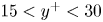


Mean velocity profiles during transition in inner units based on the local friction velocity  $u_\tau$. Linear (
 $u^{+}=y^{+}$; dashed) and log laws (
 $u^{+}=\frac {1}{0.41}\log y^{+} + 5$; dashed–dotted) are also shown. Then insets show the skin friction coefficient as a function of
 $Re_x$ and the location where the velocity profiles are plot are marked with circles. (a) Fundamental (
 $z$-symmetry). (b) Fundamental (no symmetry). (c) Superharmonic (
 $z$-symmetry).

When  $z$-reflectional symmetry is imposed, the velocity profiles show qualitatively similar characteristics as
 $Re_x$ increases, both for the fundamental and superharmonic cases. A monotonic decrease of the local streamwise velocity is observed in accordance with the monotonic increase of the skin friction coefficient. For the fundamental case with symmetry, a small logarithmic region is observed for
 $Re_x=360\,000$; however, the velocities are lower than those associated with the turbulent profile, which is in accordance with the increased skin friction coefficient beyond the turbulent values. For the superharmonic case and the forcing amplitudes examined here, the behaviour is similar without the observation of the logarithmic region. The spanwise-symmetric high-amplitude solutions calculated here that transition through streak breakdown show striking similarities with the optimal nonlinear solutions calculated in the time domain for spatially developing boundary layers. However, this is not surprising since their calculations were obtained by using a symmetric initial condition as a guess for the optimisation (Cherubini et al. Reference Cherubini, De Palma, Robinet and Bottaro2011) or spanwise symmetry was imposed (Duguet et al. Reference Duguet, Schlatter, Henningson and Eckhardt2012).
Interestingly, for the fundamental case with no symmetry in  $z$ (figure 20b), the velocity profiles at the final stages of transition show characteristics similar to the ones observed in turbulent boundary layers. Specifically, the velocity profile appears to develops a nascent logarithmic region,
 $u^{+}=\frac {1}{0.41}\log y^{+} + 5$, that extends in
 $y^{+}$ as
 $Re_x$ increases. The skin friction coefficient, after an initial overshoot above the turbulent empirical values, drops to values close to the turbulent ones. For this specific case, we observed sinuous low-speed streaks and quasi-streamwise staggered vortices, which are fundamental building blocks in the self-sustaining process in a variety of streamwise homogeneous flows (Waleffe Reference Waleffe1997, fundamental sinusoidal instability of the streaky flow), in contrast to the varicose streak instability and the hairpins that were observed for the two symmetric cases.
7. Conclusion
The nonlinear optimal mechanisms for wall-bounded laminar-turbulent transition have been investigated through the solution of the frequency-domain harmonic-balanced Navier–Stokes equations by projecting the governing Navier–Stokes equations on to a limited number of harmonics whose triadic interactions are considered. The new framework complements previous methods that seek nonlinear optimal initial conditions in the time domain within a finite time horizon. The proposed nonlinear input/output analysis identifies the most dangerous nonlinear forcing mechanisms that trigger transition and can be viewed as the minimal forcing seed in the frequency domain.
Optimal nonlinear forcing mechanisms that lead to transition and maximise the skin friction coefficient have been identified based on a variational method using direct-adjoint looping. By increasing the finite forcing amplitude, we identified the key mechanisms that distort the laminar flow and lead to transition. We showed that for fundamental forcing, the most amplified disturbances correspond to a pair of oblique waves with frequency and spanwise wavenumber close to the linear optimal one. Nonlinearity is responsible for redistributing the energy to the streamwise uniform vortex component which leads to the amplification of streaks through the lift-up mechanism. Depending on the imposed spanwise symmetry, the low-speed streaks break down to turbulence through varicose oscillations (imposing reflectional symmetry in spanwise) or sinuous-like ones (no symmetry in spanwise), with the latter being more efficient in promoting transition. In each case, hairpin vortices and quasi-streamwise vortices are observed prior to breakdown. When multi-harmonic forcing is allowed, the resonant interaction between oblique and planar waves at twice the frequency allows for even more rapid transition. At the final stages of transition, the skin friction coefficient reaches the empirical turbulent values and the velocity profiles depart from the law of the wall, for all cases examined here. However, only for the non-symmetric sinuous-like streak breakdown the velocity profiles develop a clear logarithmic region similar to the one observed for turbulent boundary layers.
Acknowledgements
We would like to thank U. Rist for providing the details for the boundary conditions used in the DNS (Rist & Fasel Reference Rist and Fasel1995). This work was initiated while D.S. was Visiting Associate at Caltech. G.R. and T.C. also acknowledge the support of the Boeing Company through a Strategic Research and Development Relationship Agreement CT-BA-GTA-1.
Declaration of interests
The authors report no conflict of interest.
Appendix A. Mesh, domain sensitivity and computational cost for $K$-type transition

A sensitivity analysis of the domain length, the finite element discretisation and the number of retained harmonics has been performed for the  $K$-type controlled transition. The amplitudes of the first few harmonics obtained by the HBM method are shown in figure 21. Mesh 1 extends to
 $x_o=2.52 \times 10^{5}$ whereas mesh 2 is for a longer domain up to
 $x_o=3.00 \times 10^{5}$. The number of triangles and degrees of freedom per harmonic of the discretised problem for the two meshes and for different choices of finite elements (
 $[P_{1b},P_{1b},P_{1b},P_{1}]$ and
 $[P_{2},P_{2},P_{2},P_{1}]$) are given in table 2. Small differences are observed in the amplitude of the various harmonics between
 $P_{1b}$ and
 $P_{2}$ elements. Given the lower computational cost (see table 3) of the former, we performed all calculations using
 $P_{1b}$ elements.
Sensitivity of various harmonics for various choices of the numerical parameters. Note that to ease representation, we have plotted one fifth of the amplitude of harmonics  $(0,\omega )$ and
 $(2\beta ,\omega )$.

Parameters for sensitivity analysis of the computational parameters.

Computational cost for HBNS solution.

Calculations were performed on a multi-node cluster, with each node having  $2\times 12$ core Xeon E5-2670 2.3 GHz CPUs and 128 GB DDR4 2133 MHz RAM. In table 3 the RAM, number of cores, number of Newton iterations for convergence and the walltime are given, depending on the order of truncation and mesh type.
Appendix B. Amplitudes of harmonics for HBM
In the  $z$-symmetric case the full solution may be rewritten under the form
 \begin{align} \hat{\boldsymbol{w}}&={\boldsymbol{w}}_b+(\hat{\boldsymbol{w}}_{00}-{\boldsymbol{w}}_b) +\sum_{m=1}^{M} (\hat{\boldsymbol{w}}_{m0}\exp({\textrm{i}m\beta z})+\mbox{c.c.})+ \sum_{n=1}^{N} (\hat{\boldsymbol{w}}_{0n} \exp({\textrm{i}n\omega t})+\mbox{c.c.}) \nonumber\\ &\quad +\sum_{m=1}^{M} \sum_{n=1}^{N} \left(\hat{\boldsymbol{w}}_{mn} \exp({\textrm{i} m\beta z+\textrm{i}n\omega t})+\hat{\boldsymbol{w}}_{-mn} \exp({-\textrm{i}m\beta z+\textrm{i}n\omega t})+\mbox{c.c.}\right). \end{align}
The domain-integrated amplitudes of the response harmonics may be defined according to
 \begin{equation} A_{\hat{\boldsymbol{w}}}(m,n) =\left\{ \begin{array}{ll} \sqrt{(\hat{\boldsymbol{w}}_{00}-\boldsymbol{w}_b)^{*}\boldsymbol{Q}'_{mn}(\hat{\boldsymbol{w}}_{00}-\boldsymbol{w}_b)} & \mbox{if } (m,n)=(0,0), \\ \sqrt{2\hat{\boldsymbol{w}}_{mn}^{*}\boldsymbol{Q}'_{mn}\hat{\boldsymbol{w}}_{mn}} & \mbox{if } (m,n) \in (0,1\ldots N) \cup (1\ldots M,0), \\ \sqrt{4\hat{\boldsymbol{w}}_{mn}^{*}\boldsymbol{Q}'_{mn}\hat{\boldsymbol{w}}_{mn}} & \mbox{if } (m,n) \in (1 \ldots M,1\ldots N), \end{array}\right. \end{equation}
where  $\boldsymbol {Q}'_{mn}$ has been defined in (5.2). The overall amplitude of all the harmonics is
 \begin{equation} A_{\hat{\boldsymbol{w}}}=\sqrt{\sum_{m \geqslant 0, n \geqslant 0} A_{\hat{\boldsymbol{w}}}(m,n)^{2}}. \end{equation}
The overall amplitude of the forcing  $\skew3\hat{\boldsymbol{f}}$ was defined in (3.16) by the
 $\boldsymbol {Q}$ matrix:
 \begin{equation} A = \sqrt{ \,\hat{\boldsymbol{f}}^{*}\boldsymbol{Q}\,\hat{\boldsymbol{f}}} = \sqrt{ \sum_{\substack{|m| \leqslant M\\ |n| \leqslant N\\ (m,n) \neq 0}} {\,\hat{\boldsymbol{f}}_{mn}^{*}\boldsymbol{Q}_{mn}\,\hat{\boldsymbol{f}}_{mn}}}. \end{equation}
In the symmetric case, noting that 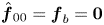 $\skew3\hat{\boldsymbol{f}}_{00}={\boldsymbol {f}}_b=\boldsymbol {0}$, following (B3), we have
 $A_{\skew3\hat{\boldsymbol{f}}}=\sqrt {\skew3\hat{\boldsymbol{f}}^{*}\boldsymbol {Q}\skew3\hat{\boldsymbol{f}}}$. The amplitudes of the individual harmonics may be represented as well with the quantity
 $A_{\skew3\hat{\boldsymbol{f}}}(m,n)$.
The maximum amplitude of any velocity or pressure component of the state vector can be calculated in accordance with (B2). For example, for the  $u$ component,
 \begin{equation} u_{max}(m,n) =\left\{ \begin{array}{ll} \max \sqrt{(\hat{u}_{00}-u_b)^{*}(\hat{u}_{00}-u_b)} & \mbox{if } (m,n)=(0,0), \\ \max \sqrt{2\hat{u}_{mn}^{*}\hat{u}_{mn}} & \mbox{if } (m,n) \in (0,1\ldots N) \cup (1\ldots M,0), \\ \max \sqrt{4\hat{u}_{mn}^{*}\hat{u}_{mn}} & \mbox{if } (m,n) \in (1 \ldots M,1\ldots N). \end{array}\right. \end{equation}
Appendix C. Link with weakly nonlinear analysis
In this appendix we analyse weakly nonlinear expansions of the HBNS solutions at low amplitudes  $A \ll 1$. We will consider two cases: § C.1 will consider the case of a fixed forcing structure composed of a single harmonic (as obtained in the case of fundamental forcing) and § C.2 the case with two harmonics (as obtained in the case of superharmonic forcing at point
 $D$ for high forcing amplitude
 $A$).
C.1. Single harmonic forcing
Suppose that the forcing only comprises a  $(\beta ,\omega )$ oblique harmonic of amplitude
 $A$ (plus the three others resulting from the
 $z$-reflectional symmetry and the real-value contraints). This forcing will be noted
 $A \skew3\hat{\boldsymbol{f}}_{11}$ in the following. For
 $A\ll 1$, considering the solution under the form (3.4), the various harmonics may be expanded as
 \begin{gather} \hat{\boldsymbol{w}}_{11}=\underbrace{A\hat{\boldsymbol{w}}_{11}^{A}}_{A\,\hat{\boldsymbol{f}}_{11}} \,+\,\underbrace{A^{3}\hat{\boldsymbol{w}}_{11}^{AAA}} _{\substack{ A\hat{\boldsymbol{w}}_{11}^{A} \,\times\, A^{2}\hat{\boldsymbol{w}}_{00}^{AA}\\ \,+\,A\hat{\boldsymbol{w}}_{-1,-1}^{A} \,\times\, A^{2}\hat{\boldsymbol{w}}_{22}^{AA}\\ \,+\,\cdots}} \,+\, O(A^{5}), \end{gather}
 \begin{gather}\hat{\boldsymbol{w}}_{02}=\underbrace{A^{2}\hat{\boldsymbol{w}}_{02}^{AA}}_{A\hat{\boldsymbol{w}}_{11}^{A} \,\times\, A\hat{\boldsymbol{w}}_{-1,1}^{A}}\,+\,O(A^{4}), \end{gather}
 \begin{gather}\hat{\boldsymbol{w}}_{20}=\underbrace{A^{2}\hat{\boldsymbol{w}}_{20}^{AA}}_{A\hat{\boldsymbol{w}}_{11}^{A} \,\times\, A\hat{\boldsymbol{w}}_{1,-1}^{A}}\,+\,O(A^{4}), \end{gather}
 \begin{gather}\hat{\boldsymbol{w}}_{22}= \underbrace{A^{2}\hat{\boldsymbol{w}}_{22}^{AA}}_{A\hat{\boldsymbol{w}}_{11}^{A} \,\times\, A\hat{\boldsymbol{w}}_{11}^{A}} \,+\, O(A^{4}), \end{gather}
 \begin{gather}\hat{\boldsymbol{w}}_{13}= \underbrace{A^{3}\hat{\boldsymbol{w}}_{13}^{AAA}}_{A\hat{\boldsymbol{w}}_{11}^{A} \,\times\, A^{2}\hat{\boldsymbol{w}}_{02}^{AA}} \,+\, O(A^{5}), \end{gather}
 \begin{gather}\hat{\boldsymbol{w}}_{31}= \underbrace{A^{3}\hat{\boldsymbol{w}}_{31}^{AAA}}_{A\hat{\boldsymbol{w}}_{11}^{A} \,\times\, A^{2}\hat{\boldsymbol{w}}_{20}^{AA}} \,+\, O(A^{5}), \end{gather}
 \begin{gather}\hat{\boldsymbol{w}}_{33}= \underbrace{A^{3}\hat{\boldsymbol{w}}_{33}^{AAA}}_{A\hat{\boldsymbol{w}}_{11}^{A} \,\times\, A^{2}\hat{\boldsymbol{w}}_{22}^{AA}} \,+\, O(A^{5}), \end{gather}
 \begin{gather}\hat{\boldsymbol{w}}_{00}=\underbrace{A^{2}\hat{\boldsymbol{w}}_{00}^{AA}}_{\substack{A\hat{\boldsymbol{w}}_{11}^{A} \,\times\, A\hat{\boldsymbol{w}}_{-1,-1}^{A}\\\,+\,\cdots}} \,+\,\underbrace{A^{4}\hat{\boldsymbol{w}}_{00}^{AAAA}}_{\substack{A\hat{\boldsymbol{w}}_{11}^{A} \,\times\, A^{3}\hat{\boldsymbol{w}}_{-1,-1}^{AAA} \\ \,+ A^{2}\hat{\boldsymbol{w}}_{20}^{AA} \,\times\, A^{2}\hat{\boldsymbol{w}}_{-2,0}^{AA}\\ \,+\, \cdots}}\,+\, O(A^{6}). \end{gather}
All non-zero terms up to order  $A^{3}$ have been indicated for
 $(m,n)\neq (0,0)$, while the development is complete up to order
 $A^{5}$ for the mean-flow harmonic
 $(0,0)$. We have shown in the underbraces a sample of forcings that trigger the considered term.
Hence, the mean friction (being a linear operator acting on  $\hat {\boldsymbol {w}}_{00}$) scales as
 \begin{equation} {\rm \Delta} C_D = {\rm \Delta} C_{D,2}A^{2}+{\rm \Delta} C_{D,4}A^{4}+\cdots. \end{equation}
C.2. Two-harmonic forcing
Suppose that the forcing lies in the  $(\beta ,\omega )$ oblique and
 $(0,2\omega )$ planar wave harmonics (plus the ones due to symmetry). Similarly to the previous section, these forcings will be noted
 $A \skew3\hat{\boldsymbol{f}}_{11}$ and
 $A \skew3\hat{\boldsymbol{f}}_{02}$. We obtain the following expansions:
 \begin{gather} \hat{\boldsymbol{w}}_{11}=\underbrace{A\hat{\boldsymbol{w}}_{11}^{A}}_{A\,\hat{\boldsymbol{f}}_{11}}\,+\,{\underbrace{A^{2}\hat{\boldsymbol{w}}_{11}^{AA}} _{\substack{ A\hat{\boldsymbol{w}}_{02}^{A} \,\times\, A\hat{\boldsymbol{w}}_{1,-1}^{A}\\ \,+\,\cdots}}}\,+\,O(A^{3}) \end{gather}
 \begin{gather}\hat{\boldsymbol{w}}_{02}={\underbrace{A\hat{\boldsymbol{w}}_{02}^{A}}_{A\,\hat{\boldsymbol{f}}_{02}}}\,+\, \underbrace{A^{2}\hat{\boldsymbol{w}}_{02}^{AA}}_{A\hat{\boldsymbol{w}}_{11}^{A} \,\times\, A \hat{\boldsymbol{w}}_{-1,1}^{A}}\,+\,O(A^{3}), \end{gather}
 \begin{gather}\hat{\boldsymbol{w}}_{20}= \underbrace{A^{2}\hat{\boldsymbol{w}}_{20}^{AA}}_{A\hat{\boldsymbol{w}}_{11}^{A} \,\times\, A\hat{\boldsymbol{w}}_{1,-1}^{A}}+\,O(A^{3}), \end{gather}
 \begin{gather}\hat{\boldsymbol{w}}_{22}= \underbrace{A^{2}\hat{\boldsymbol{w}}_{22}^{AA}}_{A\hat{\boldsymbol{w}}_{11}^{A} \,\times\, A\hat{\boldsymbol{w}}_{11}^{A}}+\,O(A^{3}), \end{gather}
 \begin{gather}\hat{\boldsymbol{w}}_{13}= {\underbrace{A^{2}\hat{\boldsymbol{w}}_{22}^{AA}}_{A\hat{\boldsymbol{w}}_{11}^{A} \,\times\, A\hat{\boldsymbol{w}}_{02}^{A}}}+O(A^{3}), \end{gather}
 \begin{gather}\hat{\boldsymbol{w}}_{04}={\underbrace{A^{2}\hat{\boldsymbol{w}}_{04}^{AA}}_{A\hat{\boldsymbol{w}}_{02}^{A} \,\times\, A\hat{\boldsymbol{w}}_{02}^{A}}}+O(A^{3}), \end{gather}
 \begin{gather}\hat{\boldsymbol{w}}_{00}= \underbrace{A^{2}\hat{\boldsymbol{w}}_{00}^{AA}}_{\substack{A\hat{\boldsymbol{w}}_{11}^{A} \,\times\, A\hat{\boldsymbol{w}}_{-1,-1}^{A}\\
\,+\,A\hat{\boldsymbol{w}}_{02}^{A} \,\times\, A\hat{\boldsymbol{w}}_{0,-2}^{A}\\
\,+\,\cdots}} \,+\,{\underbrace{A^{3}\hat{\boldsymbol{w}}_{00}^{AAA}}_{\substack{A\hat{\boldsymbol{w}}_{11}^{A} \,\times\, A^{2}\hat{\boldsymbol{w}}_{-1,-1}^{AA} \\ A\hat{\boldsymbol{w}}_{02}^{A} \,\times\, A^{2}\hat{\boldsymbol{w}}_{0,-2}^{AA}\\
\,+\,\cdots}}}+O(A^{4}). \end{gather}
These expansions are the same as for the single forcing harmonic case described in the previous section with additional terms marked in red. All terms that scale as  $A^{2}$ are given explicitly for
 $(m,n)\neq (0,0)$, while the development is valid up to order
 $A^{3}$ for the mean-flow harmonic
 $(0,0)$.
The drag increase now follows
 \begin{equation} {\rm \Delta} C_D = {\rm \Delta} C_{D,2}A^{2}+{\rm \Delta} C_{D,3}A^{3}+\cdots. \end{equation}
C.3. Scalings
Such scalings have been verified in figure 22 for superharmonic forcing at point  $D$. The red curve corresponds to the optimised solution at all amplitudes, as presented in § 6.3.
Low amplitude  $A$ scalings of drag increase in the case superharmonic forcing at point
 $D$,
 $(\beta ,\omega )=(50,11.7)\times 10^{-5}$ with
 $MN_{42}$. The red curve corresponds to the optimised solution at all amplitudes. The green curve corresponds to HBNS solutions with a fixed forcing structure corresponding to the optimal one obtained at
 $A=4.47\times 10^{-5}$ (a
 $(0,2\omega )$ planar wave plus a
 $(\beta ,\omega )$ oblique wave essentially). The green curve was produced in the same way as the blue curve, except that the chosen forcing structure corresponds to the one obtained at
 $A=5.54\times 10^{-7}$ (a pure
 $(\beta ,\omega )$ oblique forcing). Dashed lines correspond to fitting polynomial expansions for
 $A\ll 1$.

For very low amplitudes, e.g. for the leftmost point at  $A=4.54\times 10^{-7}$ on that curve in the graph, the optimal forcing is a pure
 $(\beta ,\omega )$ oblique forcing (for very low amplitudes, the cooperation between forcing harmonics vanishes and the optimal forcing converges to a single harmonic). The blue curve then corresponds to HBNS solutions with a forcing structure frozen and equal to the one obtained for
 $A=4.54\times 10^{-7}$, i.e. the above mentioned pure oblique
 $(\beta ,\omega )$ wave. Only the amplitude
 $A$ was adjusted in the various computations. For low amplitudes
 $A$, a curve fitting technique yields the scaling
 \begin{equation} {\rm \Delta} C_D=872A^{2}+5\times 10^{11}A^{4}+\cdots, \end{equation}
which is consistent with the weakly nonlinear expansion given in (C9).
For higher amplitudes, say  $A=4.47\times 10^{-5}$ (see red vertical line on the graph), the optimal forcing is essentially a combination of a
 $(0,2\omega )$ planar wave plus a
 $(\beta ,\omega )$ oblique wave. The green curve was produced in the same way as the blue curve, except that the chosen forcing structure corresponds to the one obtained at
 $A=4.47\times 10^{-5}$, i.e. the just mentioned combination between a planar and an oblique wave. Fitting this curve yields, for small amplitudes,
 \begin{equation} {\rm \Delta} C_D=225A^{2}+9.75\times 10^{6}A^{3}+\cdots, \end{equation}
which exhibits a cubic term, consistent with the development presented in (C17).
It is interesting to note that the structure of the optimal forcing at  $A=4.47\times 10^{-5}$ is strongly suboptimal at very low amplitudes: it becomes optimal only at high amplitudes due to the additional odd terms in the
 ${\rm \Delta} C_D$ development. In contrast (blue curve), the structure of the optimal forcing at very low amplitude only benefits from the even terms in the
 ${\rm \Delta} C_D$ development and becomes strongly suboptimal at high amplitudes.
Finally, note that the optimal drag increase (red curve) scales as
 \begin{equation} {\rm \Delta} C_D=872A^{2}+1.43\times 10^{12}A^{4}+\cdots, \end{equation}
which does not exhibit a cubic term. It is more difficult to justify this expansion theoretically (as done in §§ C.1 and C.2) since the forcing structure is adjusted at all amplitudes  $A$.