

1. Introduction
China has experienced explosive economic growth during the last three decades. The proportion of Chinese citizens who are urban residents increased from 20 per cent in 1980 to 40 per cent in 2004, with more than 42 per cent of the nation's population now living within 660 metropolitan regions across the country. Along with this wave of urbanization and strong economic growth, China became a far more mobile society. The country's total vehicle population increased dramatically over a five-year period, jumping from 118 million to 190 million between 2006 and 2010, an annual growth rate of 10 per cent (Ministry of Environmental Protection, 2011). As a result, residents of Chinese cities are able to travel longer distances more frequently and pursue more and more diverse travel needs.
This unprecedented growth of mobility in urban China has become an important source of air pollution and city congestion. In this paper, we use comprehensive individual travel survey data to explore what factors may affect or be associated with individual mode choices on given days. As fuel cost is likely to be an important factor in these choices and is also a direct source of emissions, in this study we investigate the impact of increasing the fuel tax on travel mode choice. The results show that if the price of gasoline is increased to a moderate level, 11.53 RMB/liter, the total car volume on the road will be reduced by 7 per cent, which corresponds to a reduction in CO2 emissions of 786,002.4 tons, or about 8 per cent of vehicular emission from private cars and company-owned cars in Beijing.
Meanwhile, we think that Beijing presents a particularly interesting case study in which to observe the relationship between transportation, regulation and air pollution, as it has been identified as ‘one of the worst environmental victims’ (Watts, Reference Watts2005: 1761). It was ranked as number one in the world in terms of the highest frequency of traffic congestion across its road network. All these problems make transportation and environmental management in Beijing a particularly salient instance of these more general problems. Therefore, we propose that the study of the relationship between transportation and its influence on air pollution in this city has two important policy contributions. First, understanding urban transportation policy experience in the Chinese context can contribute lessons and new evidence to those members of the international community facing a similar set of questions. Second, lessons from Beijing's experience can be applied to other Chinese cities which are now confronted with similar urban issues. We hope our analysis will assist others in learning lessons from the case of Beijing and, more generally, in understanding better the nexus of regulatory complexity, distortionary impacts and unexpected behavioral responses of a variety of transport policies which have been used in the city.
The outline of the paper is as follows. Section 2 introduces the existing studies on the relationship between fuel tax and air pollution. Section 3 illustrates the external cost of urban transportation in Beijing, and fuel-related policy instruments adopted in Beijing to reduce pollution externality costs. Section 4 reports results, and section 5 concludes the paper.
2. Literature review
Fuel taxes have been one of the most popular economic instruments advocated by economists to internalize the externalities from the use of motor vehicles. The simple logic behind this instrument is that the more an individual pays for negative externalities through tax, the less she would drive her vehicle on the road; how much less she would drive depends crucially on how sensitive she is to price changes.
Yet, in practice, how people respond to a fuel tax in travel demand, or how effective the fuel tax would be in alleviating traffic congestion and air pollution has not come to a common understanding. Sterner (Reference Sterner2007, Reference Sterner and Sterner2012) compares the fuel tax rates in the US and in Europe, and points out, ‘if the EU had followed a similar tax policy to that in the US, aggregate carbon emissions would have been substantially higher’, and the total fuel use would be about 30 per cent higher (Sterner, Reference Sterner and Sterner2012: 9). His data strongly suggest that fuel tax is ‘one of the few policies that actually have had a measurable effect on the carbon content of the atmosphere’ (Sterner, Reference Sterner and Sterner2012: 9). Eskeland et al. (Reference Eskeland and Feyzioglu1997: 423) use data from 31 states and the federal districts in Mexico over seven years to estimate ‘a model of gasoline demand and car ownership’ as responded to gasoline price. They find that the short-term gasoline price elasticity is −0.6, while the medium- to long-term elasticity estimates are in the range of −1.25 to −1.13 (Eskeland and Feyzioglu, Reference Eskeland and Feyzioglu1997: 423). As the car demand is responsive to fuel price change, they predict that ‘the costs of reaching a target for pollution reduction would be 45% more expensive if one were not willing to use a demand management instrument such as gasoline tax in the control program’ (Eskeland and Feyzioglu, Reference Eskeland and Feyzioglu1997: 423–424). Austin and Dinan, (Reference Austin and Dinan2005) investigate the different impacts from corporate average fuel-economy (CAFE) and fuel tax on individual travel behavior. The estimates reveal that ‘a 30 cents/gallon gasoline tax would save the same present discounted quantity of gasoline at a cost that is 71 per cent lower than the comparable CAFE policy’ (Austin and Dinan, Reference Austin and Dinan2005: 576). They also find that, compared with the more stringent CAFE standards, fuel tax would ‘accumulate savings much earlier because the tax would immediately discourage driving of new and old vehicles alike, in addition to encouraging the purchase of more fuel-efficient vehicles’ (Austin and Dinan, Reference Austin and Dinan2005: 576). In terms of the purposes of fuel tax policies, existing studies illustrate that some fuel tax policies were not originally designed to discourage the use of vehicles or to reduce fuel consumption, but rather to protect natural resources or generate greater fiscal revenue. Intention notwithstanding, Eltony (Reference Eltony1993) states that one of the observed consequences of such fuel taxes was indeed to reduce traffic volume in the short run and to push customers to switch to smaller and more fuel-efficient vehicles in the long run.
In contrast, Hughes et al. (Reference Hughes, Knittel and Sperling2008) find that the short-run price elasticity of gasoline demand has decreased in magnitude over time, ranging from −0.21 to −0.34 from 1975 to 1980, versus −0.034 to −0.077 for 2001–2006. Small and van Dender (Reference Small and van Dender2007) provide empirical evidence that the long-run price elasticity of fuel demand also declines in magnitude over time. These findings suggest that, either in the short-run or in the long-run, ‘consumers appear significantly less responsive to gasoline price increases’ today than in previous decades (Hughes et al., Reference Hughes, Knittel and Sperling2008: 115). Thus, a fuel tax ‘would need to be significantly larger today in order to achieve an equivalent reduction in gasoline consumption’, which in turn, may pose an additional hurdle to implementing fuel tax policy in practice (Hughes et al., Reference Hughes, Knittel and Sperling2008: 133). Jong and Gunn (Reference Jong and Gunn2001) summarize European literature and find that for both the short-term and long-term in European countries, the fuel price elasticities of the number of car trips are rather small, close to −0.2. In addition, commuting and business trips have even smaller elasticities in magnitude than travel for other purposes (Jong and Gunn, Reference Jong and Gunn2001: 144), indicating that these two types of trips are much less sensitive to changes in fuel prices. Sipes and Mendelsohn (Reference Sipes and Mendelsohn2001) use experimental survey data collected in Southern California and Connecticut to analyze ‘whether people would change their driving behavior in response to higher gasoline prices’ (Sipes and Mendelsohn, Reference Sipes and Mendelsohn2001: 299). The results show that either in the short run or in the long run, drivers’ demand for gasoline is price inelastic. Increasing gasoline price will ‘result in only a small reduction in driving and thus only a small improvement in the environment’ (Sipes and Mendelsohn, Reference Sipes and Mendelsohn2001: 299). Meanwhile, the financial burden induced by the increased gasoline price will fall heavily on the poor. In Japan, Tanishita et al. (Reference Tanishita, Kashima and Hayes2003) use aggregate data and a partial equilibrium model to simulate the impact of a fuel tax on air pollution. The results suggest that ‘a fuel tax is more effective than a car acquisition or ownership tax’, yet its effect on reducing fuel consumption is still limited (Tanishita et al., Reference Tanishita, Kashima and Hayes2003: 133).
As pointed out by Espey (Reference Espey1998), there is a large body of studies that have been conducted to analyze gasoline demand over the years. The results from these studies reveal that price elasticities of gasoline demand vary across regions as well as over time. But compared with the enormous amount of research in developed countries, gasoline demand in developing countries is significantly understudied. Beijing, one of the largest cities in China, is not an exception. The travel demand and related transportation policies in this city have remained poorly understood in the existing literature. The peculiar path of rapid growth, as well as the sheer size of the population and use of automobiles, suggests that Beijing is different from its Third World counterparts. The evolution of its transportation system can serve as a source of reference to facilitate a better understanding of the travel behavior in this city in particular, and in other developing economies in general. This paper is therefore a single step taken to provide preliminary and original evidence, and to analyze characteristics of the policy influence on individual travel demand and air pollution.
3. Urban transportation and policy instruments in Beijing
As the capital city of China, Beijing has experienced explosive growth over the last three decades. The total number of automobiles registered in Beijing jumped sharply from 2.583 million in 2005 to 4.809 million in 2010, of which about 3.207 million were owned by individual households. The annual growth rates for automobiles and private automobiles reached 13.2 and 19 per cent, respectively. The total number of daily trips made by the residents inside the 6th ring road of BeijingFootnote 1 was 41.30 million in 2010, of which 9.93 million (24 per cent) were made by automobiles and 11.53 million by public transit (27 per cent) (Beijing Transport Research Center, 2011a).
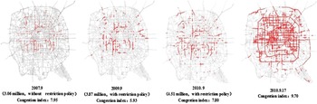
Congestion level change with 5th Ring Road, 2007–2010

However, this rapid increase in mobility comes at a high price. It has long been recognized that traffic congestion generates extraordinary negative externalities to the residents in Beijing. According to the Millennium Cities Database (MCD, 2007), Beijing was ranked as the most congested city in the world by virtue of the fact that the average travel speed in the city was the lowest among all of the cities covered by the report. Real-time intelligent transportation systems (ITS) also recorded that the average traffic congestion indexFootnote 2 in the city as a whole has increased from 5.1 during the Beijing Olympics in 2008 to 6.7 in 2010. This rating suggests that at any time on a workday, residents in Beijing are likely to encounter at least moderate congestion. This situation was even worse in the central city district surrounded by the second ring road, where the congestion index is often higher than 8. At this index value, travel speed is reduced by 50 per cent relative to average travel speeds in the rest of the city. Figure 1 illustrates how congestion in Beijing has spread out across its road network over time.
In the year 2007, congestion occurred in major commercial districts and on major arterial roads. Only three years later, congestion had spread beyond even the 6th ring road, an increase in the radius of congested areas of more than 25 km. On 27 September 2010, Beijing experienced what was widely considered to be the worst traffic jam in city history, also shown in figure 1. This congestion stretched across almost every major road, and most motorists and passengers stood in total gridlock over most of the day. All in all, congestion is now a widespread and commonly accepted circumstance of life in Beijing.
The city is paying a very high price for these high levels of congestion. Traffic jams lead to fuel wastage, higher levels of pollution, the opportunity cost of time wasted waiting in traffic, and other serious economic losses. A study conducted by Creutzig and He (Reference Creutzig and He2009) estimated that, in Beijing, the annual social cost of congestion-induced time wastage is 22.8 billion RMB for car drivers and the value of time lost in bus transportation due to congestion amounts to 5.8 billion RMB annually. In terms of air pollution, Beijing placed second globally for nitrogen dioxide (NO2), and fifth for total suspended particulates, in Gurjar et al.'s (Reference Gurjar, Butler, Lawrence and Lelieveld2008) ranking of ambient air quality among 13 of the world's megacities. In a study by Zhu et al. (Reference Zhu, Zhang, Zeng and Wang2005) the authors used a chemical mass balance receptor model and collected PM2.5 samples to test where observed pollutants originated. They found that vehicle emission has become one of the most important sources for PM2.5 in Beijing (Zhu et al., Reference Zhu, Zhang, Zeng and Wang2005). According to SEPA, vehicular emissions contributed 22.2 per cent of Beijing's levels of PM2.5 particulates. Two other studies revealed that PM2.5 from vehicular tailpipes was the major component of PM10 in the cities. The percentage composition of PM2.5 from tailpipes in ambient PM10 was 55 per cent on average in China, but reached more than 80 per cent in Beijing (Wu et al., Reference Wu, Hao, Li and Fu2002; Yang et al., Reference Yang, He, Ma, Zhang and Yu2002). Fu et al. (Reference Fu, Hao, He and He2000) applied vehicle engineering data and the MOBLE5 model in their study to find that vehicular emissions were the main contributors to air pollution in Beijing, accounting for 78, 83 and 46 per cent of CO2 HC and NOx emissions, respectively. Deng (Reference Deng2006) estimated that vehicular emissions have caused a loss of 3.26 per cent of regional GDP, comparable to the loss from congestion time wastage in Beijing.
In short, traffic congestion and its adverse impacts on air quality together constitute a substantial drain on Beijing's economy. In the last decade these have been among the most prominent concerns raised by local residents as well as policy makers in the city. In these terms, the biggest challenge facing city planners focusing on transportation in Beijing is managing the costs of the rapidly increasing volume of vehicles with the similarly increasing demand for mobility. Although this mobility has several benefits, the costs associated with these changes threaten to undo incremental gains from public investment and several other public policies.
To address urban road transportation externalities, the government of Beijing currently regulates both traffic and pollution through a combination of several policies. As early as 1998, leaded gasoline was phased out by the government. In 1999 the city government of Beijing enacted its first emissions controls on automobiles, equivalent to Euro 1 standards. One year later, Euro 2 emission standards were introduced. In the same year, to ensure that motor vehicle emission control systems were functioning properly, the city government implemented an inspection/maintenance program to perform two-speed idle tests on in-use vehicles. Beijing implemented more stringent emission standards than other comparable Chinese cities to apply to all new vehicles. For example, Euro 3 and Euro 4 standards took effect in Beijing in 2005 and 2008, respectively, while Euro 4 was introduced to the rest of the country more than two years later. To meet vehicle emission standards defined in Euro 3 and Euro 4, sulfur levels in gasoline and diesel fuel had to be reduced to 50 parts per million. The reduction of sulfur levels in diesel to the required levels posed a large challenge to China's refining industry. Nonetheless, with the implementation of this fuel economy standard, it is projected that 13 million and 31 million tons of fuel will be saved in 2020 and in 2030, respectively, according to officials from the National Development and Reform Commission.
Along with stringent regulations on new vehicles, the Beijing government implemented other policies to accelerate the retirement of old and high-emission vehicles. These policies mandate that any light-duty vehicle which fails to meet Euro 1 standards shall be subject to inspection every year and since 2003 these vehicles have not been allowed to operate inside the 2nd ring road. Through this policy, vehicle owners are encouraged to retire this type of high-polluting vehicle to avoid expensive inspection costs and restrictions on usage (Hao et al., Reference Hao, Hu and Fu2006).
The Beijing government also used economic and fiscal policies to reduce urban congestion and air pollution. Fuel tax policy is one of the examples. On 1 January 2009, China issued a new fuel tax policy which was applied to all types of vehicles including automobiles, buses and trucks. This policy took 15 years of work and cooperation among three major government agencies, namely the National Development and Reform Commission, the Ministry of Finance and the Ministry of Transport, to be implemented. It removed six types of pre-existing maintenance and management fees on roads and waterways, and instead charged a lump-sum tax. The fuel price under this scheme was raised from 0.2 RMB per liter to 1.0 RMB per liter for gasoline, and from 0.1 RMB per liter to 0.8 RMB per liter for kerosene. However, if the current elasticities (1.7 for income elasticity, and -0.65 for price elasticity) were applied in the long run and the growth rate of income was constant at 10 per cent per year (World Bank, Reference Bank2012), the price of fuel would have to rise by 28 per cent per year to keep fuel consumption constant in China. Even with more moderate figures, say, an income elasticity of 1.4, price elasticity of −0.7 and a growth rate of 7 per cent, the price of fuel would have to grow by almost 15 per cent per year, again just to keep fuel consumption and emissions constant (World Bank, Reference Bank2012). It is hard to imagine that the public would be happy with a 10 per cent increase in fuel price. Beijing is therefore in need of more comprehensive and palatable policy instruments to effectively alleviate traffic congestion and air pollution.
Besides these fuel-related policies, the municipal government of Beijing also used a one-day-a-week driving restriction policy, license plate lottery program, low fare public transport policy, transportation supply-side policies such as increased investment in transportation infrastructures, etc., to reduce negative externalities from the use of automobiles. However, most of the policies implemented in Beijing were ‘command and control’ measures. The common characteristics of these command and control measures, either in economic principles or in observed consequences, are short term, shortsighted and superficial. Any secondary responses from the public or unintended consequences, such as inventing different ways to circumvent these command and control measures, were far beyond what these policies or policy makers expected. In the long run, it is very likely that these command and control measures could create perverse incentives leading to more severe congestion and pollution. This then left the government with very few effective options except economic instruments to explore, including a higher and flexible gasoline tax, higher and flexible parking fees and a congestion fee. This paper illustrates how one type of economic instrument, namely a gasoline tax, can effectively reduce use of vehicles and related air pollution. Our approach is to estimate a behavior model of transportation mode choice, and use the estimates to simulate effects of a gasoline fee on vehicle use pattern change and its consequent changes in air pollutant emissions.
4. Results
4.1. Survey and construction of alternative transport choice sets
The data used in this study are from the Beijing Household Travel Survey. This survey was conducted in September and October of 2010 by the Beijing Transportation Research Center.Footnote 3 Holiday periods (22–24 September and 1–7 October) in those two months were excluded. All respondents in the sample took the face-to-face interviews at their homes and were asked to report their travel in a one-day trip diary.
To analyze travel mode choice in Beijing, the sample used in the study consists of individuals, currently employed and working outside of the home, who have access to a car during the peak hours of the morning (7–9 a.m.).Footnote 4 Like most other cities, the congestion level in Beijing during these peak hours is the worst. We used the commute to work, or ‘simple work trip’, as the main object of our inquiry. A simple work trip is defined as a trip starting from home and arriving at the respondent's workplace with the single goal of working. In total, we have 3,435 working trip observations from 2,726 households eligible for our final analysis.
We should note that it is very important to accurately measure travel distance to calculate the time and cost of alternative transport choice sets. The data itself do not contain the reported commuting distance information. We therefore, in accord with most of the available literature, calculated the distance of the shortest path (the so-called Euclidean distance) between the two locations (home and workplace) using GIS.Footnote 5
Possible alternative transport mode choices include bicycle, bus, subway, car, taxi, motorcycle, company-owned bus and walking. We exclude motorcycle and company-owned bus as alternative choices given that the number of such observations is quite small. We also do not consider walking for the final analysis because of significant measurement errors in distance when we use GIS to locate the home and workplace address.Footnote 6 Another important issue is how to construct trip attributes of alternative transport mode choices. We do this by using Euclidean distance calculated through GIS information and average community trip information. We first calculate the cost for each mode. We set the monetary cost of a trip to be zero for biking and 2 RMB for taking the subway. The cost of taking a taxi is easily calculated from the travel distance. In Beijing, the taxi fee is 10 RMB for trips within 3 km. A 2-RMB-per-km rate is charged for any travel distance from 3 to 15 km. And then a 1-RMB-per-km rate is set for any distance beyond 15 km of the total travel distance. The bus fee is settled by the public transport authority at 0.2 RMB for students, 0 for elderly people holding a Senior Citizen Certificate, 0.4 RMB for people with public transportation cards, and 1 RMB for people without public transportation cards. Fuel costs are calculated based on a uniform average speed of 20 km/hour and travel distance. We use 0.075 liter/km as average fuel consumption per unit of distance, and 6.87 RMB/liter as fuel price in 2010 (Song et al., Reference Song, Yu and Wang2008). The fuel cost is then equivalent to commuting distance multiplied by 0.515 RMB/km. The journey time for each transport mode is obtained by dividing commuting distance by average speed. In our sample, we have 250,000 trip observations.Footnote 7 We calculate the average speed for each mode based on these observations from each neighbor community (approximately Jie Dao in Chinese). This average speed is then used to calculate the in-vehicle time for respondents living within this community. For out-of-vehicle time, such as walking and waiting times for the bus, time spent walking to the location of a parked car, and waiting and walking time for using the subway, we use the time value averaged from each neighbor community. In addition, all time not spent in vehicles is defined as out-of-vehicle time.
4.2. Variables and regression results description
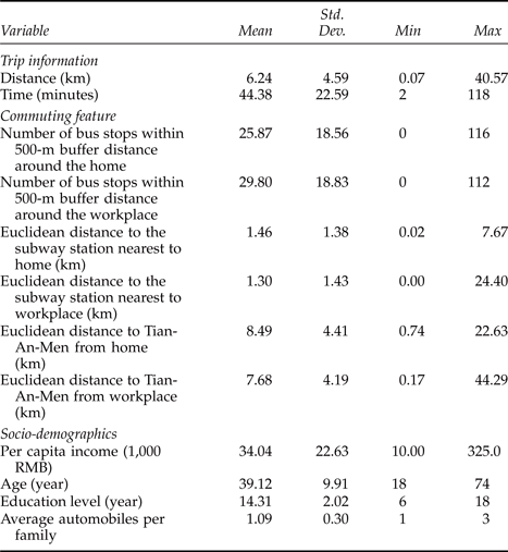
In this study, we use Random Parameter Logit Model (RPL) to analyze individual travel mode choice (technical details regarding the RPL model are given in Appendix A). In general, there are three types of factors considered to influence the respondent's transport mode choice: the first type of factor is trip attributes such as time and cost of a transport mode; the second is the individual's social and demographic characteristics such as age, gender, per capita income and education level; and the third type includes trip-related locational factors, including distance to subway and distance to city center. Table 1 provides a list of these variables and reports descriptive statistics of the sampled households.
Descriptive statistics

The results show that the per capita income is about 34,000 RMB. The average age of respondents is about 39, and respondents have on average about 14 years of education. Since our sample focuses on families with cars, the average number of automobiles per family is larger than 1. More specifically, 5.65 per cent of families in our sample have two cars, and 0.15 per cent of families have three cars. The data show that 51 per cent of respondents do not use cars to commute in our observed trips. The average commuting distance is 6.24 km. On average, respondents spend around 45 minutes on the morning trip to work.
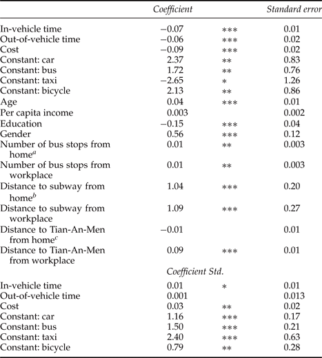
The results of the RPL model are reported in table 2. They are estimated with simulated maximum likelihood using Halton draws. The estimated standard deviations of the random parameters were significant, implying that we were able to capture most unobserved heterogeneity, with ‘out-of-vehicle time’ as the exception. The coefficients on trip attribute are negative, which is consistent with our expectations, indicating that if the cost or in-vehicle time/out-of vehicle time increases, the probability of choosing that particular transport mode will decrease. The alternative-specific constant was negative and significant for taxis, indicating that respondents would rather take the subway than a taxi. In contrast, the signs are uniformly significant and positive for taking cars, buses and bicycle, suggesting that our respondents are less likely to prefer taking the subway compared to these three transport modes. As expected, when public transport infrastructure is better developed for the trip between the home and workplace, respondents are more likely to take the bus and subway. This is reflected by the positive coefficients on variables such as distance to subway from home/workplace and number of bus stops within a 500-m buffer distance around the home/workplace. The negative and significant sign for ‘Distance to Tian-An-Men from workplace’ suggests that respondents tend to commute to their workplaces via the subway if the workplace is closer to the city center as proxied for proximity to Tian-An-Men. This is reasonable since, both empirically and anecdotally, traffic is far more congested in the places closer to the city center. Therefore, to get to work in time, it is more likely that the respondent will choose a transport means with a more predictable arrival time such as the subway.
Random parameter logit estimation results
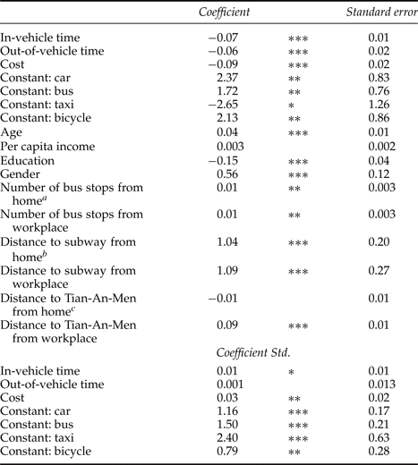
Notes: Subway is taken as a reference alternative for other transport modes: car, bus, taxi and bicycle
a We only consider variables ‘Number of bus stops from home/workplace in the utility function for bus.
b Similarly, variables ‘Distance to subway from home’ are only considered in the utility function for taking the subway.
c Variables ‘Distance to Tian-An-Men from home/workplace’ enter the utility function by interacting with the alternative-specific constant.
***, **, * significant at the 1%, 5% and 10 levels, respectively.
4.3. Simulation of fuel tax rise
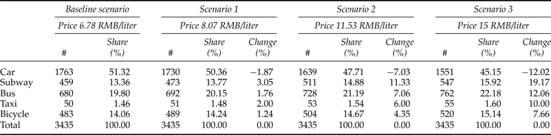
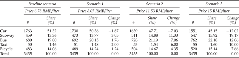
Now we turn to simulating the impacts on travel mode from a fuel tax rise. This is done by changing the value of fuel costs on cars in the model. If we impose a fuel tax on gasoline, the tax will drive up the gasoline price correspondingly. The gasoline price at the time of the survey was 6.78 RMB/liter, which we take as our baseline scenario. For our fuel tax simulations, we use three different scenarios. In scenario 1, the gasoline price is increased to 8.07 RMB/liter, or a 19 per cent increase (equivalent to 2012 gasoline prices in Beijing); and in scenario 3, we increase the gasoline price to a much higher level of 14.93 RMB/liter, or a 120 per cent increase (equivalent to gasoline prices in Hong Kong). We also set a moderate-level fuel price for scenario 2, which is 11.53 RMB/liter or about a 70 per cent price increase.
The impacts of transport mode changes are presented in table 3. The simulation results show that if the gasoline price increases by 19 per cent (scenario 1), the share of private cars changes only slightly, falling by 1.87 per cent. This is consistent with the anecdotal evidence. When the gasoline price increased to 8.07 RMB/liter in 2012 from 6.87 RMB/liter in 2010, the impact on the travel mode choice with car is not very noticeable. In other words, the price impact on car users is very small. If the gasoline price increases by 70 per cent, the impact is relatively larger and the share of private vehicle decreases by 7 per cent. Furthermore, if gasoline increases to the Hong Kong price level (scenario 3), the share of private car use declines substantially, by about 12 per cent.
Simulation of fuel tax rate rise
4.4. Impact on vehicular emissions with transport mode changes
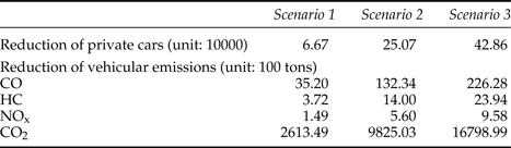
As a next step we are able to calculate changes in vehicular emissions as a result of different fuel tax levels. According to the Beijing Transport Annual Report (2011b), the total number of motor vehicles is 4.8 million, of which 3.56 million are private vehicles. Since we already know the amount of private vehicle change associated with our three different scenarios from the simulations (see table 3), we can then use these to calculate the number of private cars reduced under each scenario. These results are presented in table 4. Reduction of vehicular emissions is calculated based on the following equation:
 $$\eqalign {&\hbox{Vehicular emissions} = \hbox{vehicle population} \times \hbox{emission factors}^8 \cr & \quad \times \hbox{vehicle miles travelled annually}.}$$
The total estimated vehicular emission reductions are shown in table 4.
The impact on vehicular emissions reductions

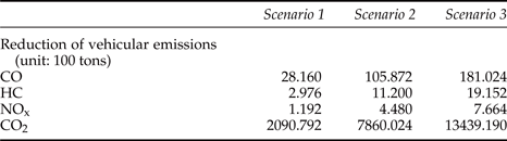
We are certainly aware that an individual completely ceasing to drive if the fuel tax increases is an unrealistic assumption. We thus assume that respondents would not abandon their cars completely, but would rather drive during the weekend. We find that under this scenario the vehicle miles travelled annually would decrease by 20 per cent (assuming vehicle miles travelled during the working days account for about 80 per cent of total travelling miles). These results are presented in table 5.
The impact on vehicular emissions reductions (only drive at the weekend)

According to the Beijing Transportation Committee, energy consumption for private and company-owned cars is about 4.86 million tons of the standard coal equivalent. If we use 2.4567 tCO2/tce as a CO2 conversion coefficient (National Development and Reform Commission), total vehicular emissions are about 11.93 million tons. As a result, the vehicular emission reductions due to the fuel tax rises in scenarios 1, 2 and 3 would account for about 2, 8 and 15 per cent of this decrease, respectively.
5. Conclusions
As an international metropolitan area under rapid development, Beijing is facing a sharp rise in its vehicle population. While its residents have enjoyed great benefits from this increase in mobility, they and their neighbors are also paying a heavy price. Beijing is already one of the world's most polluted cities in terms of air quality, and vehicular emissions contribute heavily to levels of hazardous local air pollutants such as carbon monoxide (CO), oxides of nitrogen (NOx), and volatile organic compounds (VOCs). The city has been named by numerous international organizations as among the most congested in the world, and both the extensive economic costs of this congestion and the links between the increase in vehicle traffic, congestion and pollution have been well documented.
These facts raise the question of what to do about the problem. More specifically, how do policy makers balance the benefits of continued improvements in mobility with the costs of pollution and congestion? In answer to this question, the Beijing Government has adopted a battery of policy instruments in an attempt to reduce the negative transport externalities so apparent in the city. So far, the results have been limited. We argue that economic instruments such as fuel taxes can be more effective in combating vehicle pollution, global warming and other externalities such as congestion and car accidents.
In this study, we estimated a model that predicted the results of increasing the fuel tax on pollution and congestion in an attempt to provide information to those who have to deal with these problems. Our preferred results show that if the gasoline price increased to 11.53 RMB/liter (a moderate level), a 70 per cent increase over the 2010 gasoline price in Beijing, then the overall car share will be reduced by 7 per cent. Correspondingly, the CO2 emissions will be reduced by 786,002 tons, which is about 8 per cent of vehicular emission from private cars and company-owned cars in Beijing. Furthermore, if the gasoline price increased to 15 RMB/liter, a 120 per cent increase over the 2010 gasoline price in Beijing, then the overall car share will be reduced by a much greater percentage, about 12 per cent.
Politically speaking, local governments in China as well as in other developing countries often favor a command-and-control type of traffic restriction policy. Road restriction policies implemented in Beijing and several other cities in Central America are a good example of such policies. Our work suggests economic instruments could be far more effective than such more administratively demanding policy initiatives both in reducing CO2 emissions and in changing residents’ incentives to use cars vis-à-vis other methods of commuting. We hope the effectiveness of this policy instrument demonstrated by this study will be used to form transportation policy which properly aligns incentives for balancing the costs and benefits of the rapid increase in mobility that the residents of Beijing have experienced.
We are also aware that it is still difficult to reach the vehicle population and air pollution goals set by the municipal government by relying upon a single policy instrument such as fuel tax. For example, even with a dramatic rise in price by 120 per cent or equivalent to Hong Kong gasoline price levels, our simulation results show that total number of vehicles on the road could be reduced by 12 per cent in Beijing. This 12 per cent reduction of car use might not seem to be as effective as a traffic restriction policy which was supposed to take one-fifth of the vehicles off the road on every workday, not to mention that it is hard to imagine that the public would be happy with a more than 100 per cent increase in fuel price. As such, Beijing is in need of more comprehensive and palatable policy instruments (e.g., congestion tolls, parking fees) to effectively alleviate traffic congestion and air pollution.
Appendix A
In the analysis of the choice responses, we apply a random parameter logit model in which taste variation among individuals is explicitly treated. We could write the utility function of alternative i for individual n as:
 $$v_{in} = \beta a_i + \varepsilon_{in} = \bar{\beta} a_i + \tilde{\beta}_n a_i + \varepsilon_{in}$$
Each individual's coefficient vector β is the sum of the population mean
 $\bar{\beta}$
and individual deviation
 $\bar{\beta}_{n}$
. The coefficients (the preferences) vary in the population with density
 $f(\beta \vert \theta)$
, where θ is a vector of the true parameters of the taste distribution. If the error terms follow IID type I extreme value, the model is called a random parameter logit model. The conditional probability of alternative i for individual n is expressed as:
 $$L_{n} (i \vert \beta) = \displaystyle{{\exp (\beta a_i/\tau)} \over {\sum \exp (\beta a_i/\tau)}}$$
The unconditional probability of an alternative i for individual n is then the integral of the conditional probability over all values of β:
 $$P(i \vert \theta) = \int L_n (i \vert \beta) f (\beta \vert \theta) d\beta = \int \displaystyle{{\exp (\beta a_i/\tau)} \over {\sum \exp (\beta a_i/\tau)}} f(\beta \vert \theta) d \beta$$
In general, the integrals could not be evaluated, and we have to rely on a simulation method for the probabilities. We here use Halton draws to estimate the models (Train, Reference Train1999). In brief, the estimator can be described as follows. From a given distribution θ, individual specific values of β are drawn. From these draws we approximate the choice probability using the standard logit. In order to estimate the model, it is also necessary to make an assumption regarding the distribution of each of the random coefficients. In theory, we could assume and apply any distribution. However, we often use two main alternative assumptions in practice, that is, normal and log-normal distribution (Carlsson et al., Reference Carlsson, Frykblom and Liljenstolpe2003). Applying a log-normal distribution means that we restrict all respondents to having the same sign of each coefficient. In our case, we assume that the random coefficients are normally distributed, and this means that we did not restrict the sign of a coefficient to be only negative or only positive. In addition, we treated time (including in-vehicle and out-of-vehicle time), price and alternative specific constant as random variables. In a random parameter logit model, the significance of the estimated standard deviations is a sign of heterogeneity in preference among individuals.
Appendix B: Transportation survey questionnaire (major questions)
1. Family characteristics
-
(1) Home address
-
(2) Size of the family
-
(3) Number of family members who are currently working
-
(4) Family annual income
-
(5) Number of cars owned by the family
-
(6) Number of bicycles owned by the family
-
(7) Number of motorcycles owned by the family
-
(8) Number of powered two-wheelers owned by the family
2. Individual characteristics (for each family member)
-
(1) Year of birth
-
(2) Hukou type
-
(3) Education level
-
(4) Full-time or part-time work
-
(5) Occupation
-
(6) Industrial sector of the job
-
(7) Type of driver's license
-
(8) Public transportation pass
3. Characteristics for each automobile used in the family
-
(1) Ownership rights of the automobile: privately or organization owned
-
(2) Type of automobile: car, SUV, van, truck, etc.
-
(3) Major user
-
(4) Last digit of the license plate number
-
(5) Average monthly fuel cost
4. 24-hour trip diary
-
(1) The date
-
(2) Where were you at 3:00 a.m. on that day? (street address)
-
(3) What did you do there?
-
(4) When did you leave?
-
(5) Where did you head for?
-
(6) Which transportation mode did you use?
-
(7) How much did you pay out of your pocket through this trip? (including toll fee, parking fee, etc.)
-
(8) How many minutes did you spend walking to the bus/subway station or to the automobile?
-
(9) How many minutes did you spend waiting for public transit?
-
(10) When did you arrive?
-
(11) Is this your final station? If not, then continue with questions 3 to 10.