1. Introduction
The Lagrangian particle dispersion model (LPDM) is a key scientific tools underpinning our quantitative understanding of the dispersal of trace-gas pollutants and aerosols in turbulent flows. Applications in atmospheric and oceanic science are numerous. Examples include establishing the relationship between emissions of pollutants and air quality downstream (Cassiani, Stohl & Eckhardt Reference Cassiani, Stohl and Eckhardt2012), modelling aerosol dispersal following volcanic eruptions (D'Amours et al. Reference D'Amours2010; Devenish et al. Reference Devenish2011), modelling of nuclear accident scenarios (Stohl, Seibert & Wotawa Reference Stohl, Seibert and Wotawa2012) and determination of constraints on chemical emissions via inverse modelling (Seibert & Frank Reference Seibert and Frank2004; Stohl et al. Reference Stohl2010).
Typically, the LPDM is used to solve ‘random flight’ stochastic differential equations for particle position  $\boldsymbol {X}$ and velocity
 $\boldsymbol {U}$ of the form
 \begin{equation} \left. \begin{aligned} \textrm{d} \boldsymbol{U} & = \boldsymbol{a}( \boldsymbol{U},\boldsymbol{X},t) \, \textrm{d}t + \left( 2 \boldsymbol{\mathcal{B}}( \boldsymbol{U}, \boldsymbol{X},t) \right)^{1/2} \boldsymbol{\cdot} \textrm{d} \boldsymbol{W}, \\ \textrm{d}\boldsymbol{X} & = \boldsymbol{U} \, \textrm{d}t. \end{aligned} \right\} \end{equation}
Here,  $\boldsymbol {a}(\boldsymbol {u},\boldsymbol {x},t)$ is the particle acceleration and
 $\boldsymbol {\mathcal {B}} ( \boldsymbol {u}, \boldsymbol {x},t)$ is a symmetric, positive definite matrix-valued function which determines the random turbulent increment, which is driven by the vector-valued Brownian (or Wiener) process
 $\boldsymbol {W}$.
In stationary homogeneous isotropic turbulence, suitable choices for  $\boldsymbol {a}$ and
 $\boldsymbol {\mathcal {B}}$ can be constrained by considering the statistics of Lagrangian time series
 $(X(t), U(t))$ of a single component of the position and velocity vector in a general turbulent flow. The exact result of Taylor (Reference Taylor1921), for the time evolution of the variance in particle position, which follows from integration of the trajectory equation, is
 \begin{equation} \frac{\textrm{d}}{\textrm{d}t} \langle X^2 \rangle= 2 \sigma^2 \int_0^t R_{uu}(t-s) \, \textrm{d}s, \end{equation}
where, using angle brackets to denote ensemble averages,  $\sigma ^2=\langle U^2 \rangle$ is the velocity variance and
 $R_{uu}(s)=\langle U(t) U(t+s) \rangle / \sigma ^2$ is the Lagrangian velocity autocorrelation, from which the Lagrangian decorrelation time scale
 \begin{equation} \tau = \int_0^\infty R_{uu}(s) \, \textrm{d}s \end{equation}
can be defined. The simplest model in the class (1.1) which is consistent with Taylor's description is the Ornstein–Uhlenbeck process
 \begin{equation} \textrm{d} \boldsymbol{U} ={-}\frac{\boldsymbol{U}}{\tau} \, \textrm{d}t +\left( \frac{2 \sigma^2}{\tau} \right)^{1/2} \, \textrm{d} \boldsymbol{W}. \end{equation}
In the stationary state the Ornstein–Uhlenbeck process (1.4) has Gaussian single-point velocity statistics, and Lagrangian autocorrelation  $R_{uu}(s)=\textrm {e}^{-s/\tau }$, which is a reasonable fit to measurements in grid turbulence (see e.g. the review of experimental data in Pope Reference Pope1994). The time scale
 $\tau$ is determined by comparing the quadratic variation in (1.1),
 $\langle \textrm {d} \boldsymbol {U} \,\textrm {d}\boldsymbol {U}^{\textrm {T}} \rangle = 2 \boldsymbol {\mathcal {B}} \, \textrm {d}t$, with the corresponding Lagrangian structure function
 $\langle \delta \boldsymbol {u} \, \delta \boldsymbol {u}^{\textrm {T}} \rangle$ in the turbulent flow, where
 $\delta \boldsymbol {u}= \boldsymbol {u}(t+\delta t)-\boldsymbol {u}(t)$. In the similarity theory of Kolmogorov–Obuhkov (see p. 358 of Monin & Yaglom Reference Monin and Yaglom1975), the structure function in stationary homogeneous isotropic turbulence has the universal form
 \begin{equation} \langle \delta \boldsymbol{u} \, \delta \boldsymbol{u}^{\textrm{T}} \rangle = C_0 \epsilon \, \delta t \, \boldsymbol{\mathcal{I}}, \end{equation}
where  $\epsilon$ is the energy dissipation rate,
 $C_0$ is the Lagrangian velocity structure function inertial sub-range constant (e.g. Sawford, Pope & Yeung Reference Sawford, Pope and Yeung2013), which is non-dimensional and universal in theory (in practice a value in the range 3–7 is fitted to data). Note that the time interval
 $\delta t \gtrsim t_\nu \equiv (\nu /\epsilon )^{1/2}$ (the Kolmogorov time scale). It follows that
 $\boldsymbol {\mathcal {B}} = (C_0 \epsilon \boldsymbol {\mathcal {I}})/2$ and
 $\tau = 2\sigma ^2(C_0 \epsilon )^{-1}$. It is important to note the caveat that, while the model (1.4) is extremely useful owing to its simplicity, it cannot of course capture the full complexity of single-point statistics even in stationary isotropic turbulence, in particular the intermittency evident in higher-order Lagrangian structure functions (Arnèodo et al. Reference Arnèodo2008).
In inhomogeneous or unsteady turbulence, however, it is less clear how to choose a suitable model (1.1). In most previous research (see e.g. the review by Thomson & Wilson Reference Thomson and Wilson2013), it assumed that the single-point velocity probability density function for the fluid is known everywhere (e.g. from measurements), and that  $\boldsymbol {\mathcal {B}}$ is also known, e.g. Kolmogorov's hypothesis of local isotropy suggests using the homogeneous value
 $\boldsymbol {\mathcal {B}} = (C_0 \epsilon \boldsymbol {\mathcal {I}})/2$ (e.g. Borgas, Flesch & Sawford Reference Borgas, Flesch and Sawford1997). The question is then how best to choose
 $\boldsymbol {a}$ to capture the statistics of particle dispersion consistently. The problem is motivated in large part by the situation in the atmospheric boundary-layer in which there is both a mean flow and a vertical gradient in the turbulent statistics. The key breakthrough in understanding, owing to Thomson (Reference Thomson1987, T87 hereafter), was the realisation that
 $\boldsymbol {a}$ must be chosen to satisfy the ‘well-mixed condition’, detailed in § 2. Essentially, the well-mixed condition ensures that, at late times, the probability distribution for the velocity and distribution of a particle evolving according to (1.1) will converge to the distribution that has been specified for the fluid. In the case of an incompressible fluid in a bounded domain, the fluid distribution requires the particles at late times to be uniformly distributed in space. Models which do not satisfy the T87 well-mixed condition have the unphysical property that particles tend to drift and accumulate in certain regions of the domain, e.g. near the ground in an atmospheric boundary-layer model.
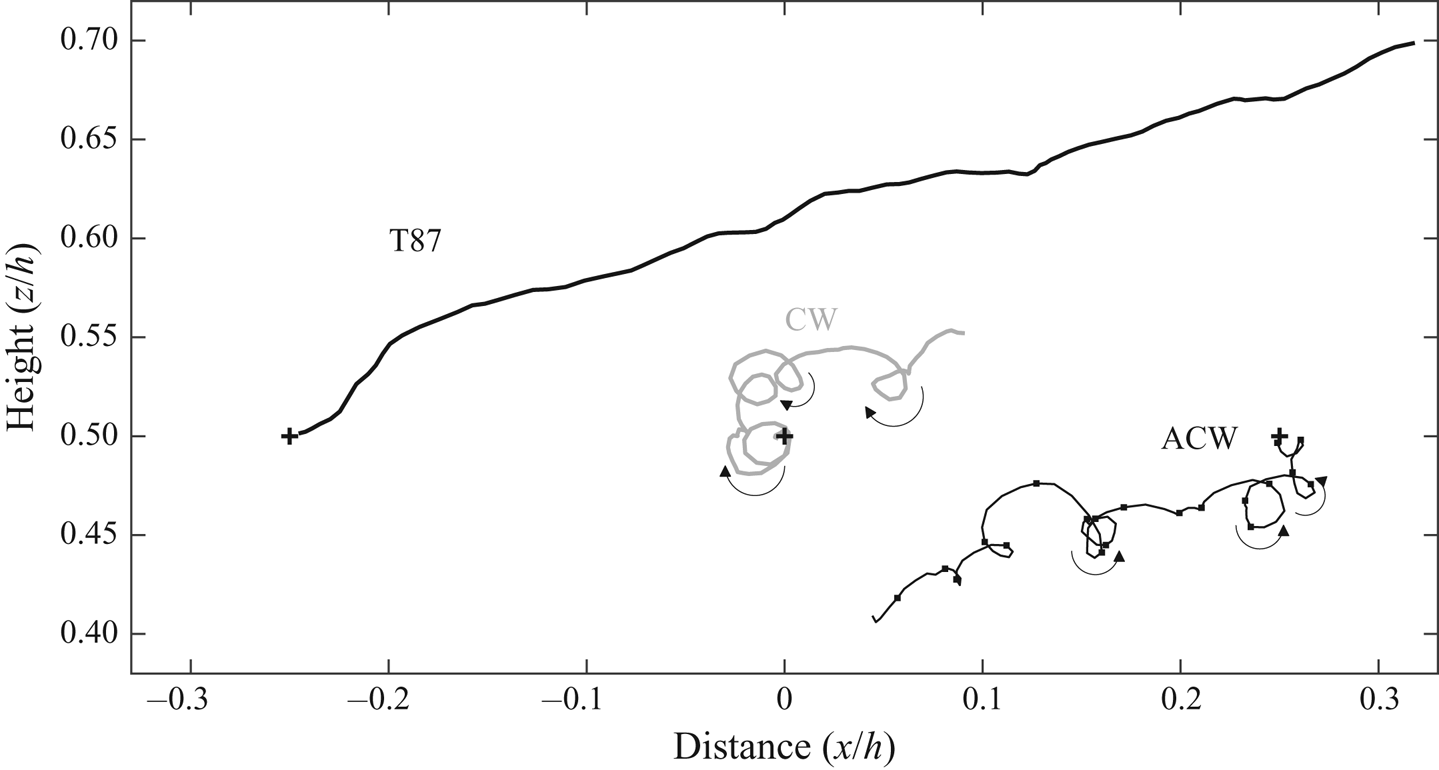
In one dimension T87 showed that the well-mixed condition is sufficient to determine  $\boldsymbol {a}$ uniquely. In two or more dimensions, however, well-mixed models are not unique. The non-uniqueness is known to be related to the rotational degrees of freedom available to trajectories (Sawford & Guest Reference Sawford and Guest1988). Previous attempts to constrain the models based on criteria such as trajectory curvature and rotation rate (Wilson & Flesch Reference Wilson and Flesch1997; Reynolds Reference Reynolds1998; Sawford Reference Sawford1999) have been inconclusive. It is straightforward to construct examples of well-mixed models in order to demonstrate that the rotational degrees of freedom allow for models which are unphysical. Figure 1 shows sample trajectory paths from three integrations of (1.1), for models – detailed in § 4.2 – which have different choices of
 $\boldsymbol {a}$ that satisfy the T87 well-mixed criterion in the presence of a uniform shear flow. The model T87 is that proposed by Thomson (Reference Thomson1987), while models ACW (anticlockwise) and CW (clockwise) are by design absurd. Model ACW generates trajectories which undergo rapid anticlockwise rotation, counter to the direction of the shear, whereas for model CW the trajectories rapidly rotate clockwise with the shear. Borgas et al. (Reference Borgas, Flesch and Sawford1997) have shown that such spurious rotation acts to suppress particle dispersion to an unphysical extent (see also Esler & Ramli Reference Esler and Ramli2017, for a full treatment of the effect in the shear dispersion problem). A related unphysical feature of the models CW and ACW is that velocity autocorrelation functions, such as
 $R_{uu}$ defined earlier, exhibit oscillations.
Example trajectories of duration  $t=hu_*^{-1}$ from three different well-mixed models of dispersion in an atmospheric boundary layer. Model details are given in § 4.

The rationale for this work is the observation that there is a simple physical argument governing the ‘expected’ rotation rate of trajectories (in a sense to be made precise later) such as those shown in figure 1. The rationale is as follows: the expected angular velocity of a trajectory, measured relative to the local ensemble mean trajectory, should be  $\bar {\boldsymbol {\omega }}/2$, where
 $\bar {\boldsymbol {\omega }}$ is the vorticity of the mean flow. The rationale for this statement is simply that
 $\bar {\boldsymbol {\omega }}/2$ is the local angular velocity of particles in the mean flow. For example, consider a turbulent flow with a mean velocity corresponding to solid-body rotation flow about the origin, with constant angular velocity
 ${\boldsymbol {\varOmega }}$. The mean velocity is
 $\bar {\boldsymbol {u}}={\boldsymbol {\varOmega }} \times \boldsymbol {x}$, from which the (mean) vorticity is easily calculated to be
 $\bar {\boldsymbol {\omega }} = 2{\boldsymbol {\varOmega }}$ everywhere. Self-evidently, in such a flow, the expected angular velocity of the particle trajectories should be
 ${\boldsymbol {\varOmega }}$. Subsequently, it will be shown that the acceleration term in (1.1) consistent with this outcome is
 $\boldsymbol {a}_r=2{\boldsymbol {\varOmega }} \times (\boldsymbol {u}-\bar {\boldsymbol {u}})$, which can be recognised as the Coriolis acceleration familiar from rotating fluid dynamics, applied to the velocity perturbation
 $(\boldsymbol {u}-\bar {\boldsymbol {u}})$. Generalising to flows with spatially and temporally varying mean vorticity, the corresponding term can be expected to be
 \begin{equation} \boldsymbol{a}_r=\bar{\boldsymbol{\omega}} \times (\boldsymbol{u}-\bar{\boldsymbol{u}}). \end{equation}
The spin condition, introduced later to determine  $\boldsymbol {a}$ uniquely in three dimensions, invariably leads to (1.6) being the undetermined linear (in
 $\boldsymbol {u}-\bar {\boldsymbol {u}}$) term in
 $\boldsymbol {a}$.
It is important to emphasise that the T87 approach in determining the LPDM is not the only one available. In the turbulence-modelling approach pioneered by Haworth & Pope (Reference Haworth and Pope1986), (see also the review of Pope Reference Pope1994), semi-empirical generalised Langevin models (GLM) of the form (1.1) are proposed, and are used to derive, rather than specify, the associated evolution equations for the mean velocity and the velocity covariance matrix. The turbulence-modelling approach is evidently important, but will not be our focus here, beyond some brief speculations on the possible role of the spin condition in constraining components of the GLM.
The plan of the work is as follows. In § 2 Thomson's well-mixed condition is reviewed and the mathematical problem to be solved is defined. In § 3 the spin condition is stated, and strong and weak versions are defined. The strong spin condition is then used to obtain the unique strong spin well-mixed canonical model for flows with Gaussian single-particle distributions. Particle accelerations in the strong spin model can be large, so a weak spin condition is introduced in order to obtain the unique weak spin well-mixed canonical model which, unlike the strong spin model, is quadratic in the velocity perturbation. The behaviour of the models is discussed first for the important example of homogeneous isotropic turbulent flow in solid-body rotation, and then for the case of a neutral atmospheric boundary layer with uniform vertical shear, in § 4. In § 5 conclusions are drawn.
2. Thomson's well-mixed condition and the uniqueness problem
2.1. Mathematical notation
The work in this section is necessarily mathematical, so some advance comments on the notation to be used may prove helpful. Throughout, non-stochastic scalar fields, vector fields, matrices and tensors will be denoted using lower-case italics, lower-case bold, upper-case bold script and upper-case script, e.g.  $f$,
 $\boldsymbol {v}$,
 $\boldsymbol {\mathcal {C}}$,
 $\mathcal {Q}$, respectively. Stochastic scalars and vectors will be denoted using upper-case, e.g.
 $U$ and
 $\boldsymbol {X}$, respectively.
The mathematics repeatedly references ideas from vector calculus, hence a notation is adopted which emphasises that, i.e. index notation will be used sparingly. Contractions between vectors (including the vector operator  $\boldsymbol {\nabla }$) and matrices are denoted by the dot product, e.g.
 $\boldsymbol {\mathcal {C}} \boldsymbol {\cdot } \boldsymbol {v}$. For contractions over two indices the double dot
 $:$ will be used. Where outer products are intended dots are omitted, as are transposes on vectors and matrices (except for certain expressions involving the gradient operator). To give some examples, let
 $v_i$,
 $C_{ij}$ and
 $Q_{ijk}$ denote the components of
 $\boldsymbol {v}$,
 $\boldsymbol {\mathcal {C}}$ and
 $\mathcal {Q}$, respectively. Then
 $\boldsymbol {v} \boldsymbol {\cdot } \boldsymbol {\mathcal {C}} \boldsymbol {\cdot } \boldsymbol {v}$ and
 $\boldsymbol {\nabla } \boldsymbol {\nabla } : \boldsymbol {\mathcal {C}}$ denote the scalar fields
 $v_iC_{ij}v_j$ and
 $\partial _i \partial _j C_{ij}$, where
 $\partial _i$ here denotes the partial derivative in physical space in the
 $i$th direction (Einstein summation convention implied). Further,
 $\mathcal {Q}:\boldsymbol {v} \boldsymbol {v}$ is a vector with components
 $Q_{ijk}v_jv_k$, and
 $\boldsymbol {v} \boldsymbol {\cdot } \boldsymbol {\nabla } \boldsymbol {\mathcal {C}}$ is a matrix with components
 $v_k \partial _k C_{ij}$, etc.
While the vector calculus notation adopted allows for a somewhat neater presentation of the main results, and makes aspects of the mathematics easier to follow, it is nevertheless useful on occasion to switch to the index notation.
2.2. The well-mixed condition applied to the general model
Consider the class of Lagrangian particle dispersion models defined by (1.1). Standard results of stochastic calculus (see e.g. Gardiner Reference Gardiner2009, § 3.4.1) reveal that the probability density  $p(\boldsymbol {u},\boldsymbol {x},t)$ of the random variables
 $(\boldsymbol {U},\boldsymbol {X})$ evolves according to the 6+1 dimensional Fokker–Planck equation
 \begin{equation} \partial_t p + \boldsymbol{\nabla} \boldsymbol{\cdot} (\boldsymbol{u} p) + \boldsymbol{\nabla}_{\boldsymbol{u}} \boldsymbol{\cdot} (\boldsymbol{a} p) - \boldsymbol{\nabla}_{\boldsymbol{u}} \boldsymbol{\nabla}_{\boldsymbol{u}} : (\boldsymbol{\mathcal{B}} p) =0, \end{equation}
where  $\boldsymbol {\nabla }$ denotes the gradient operator in physical space and
 $\boldsymbol {\nabla }_{\boldsymbol {u}}$ in velocity space.
The starting point for the construction of the T87 well-mixed condition is the knowledge of a known fluid distribution  $p_f(\boldsymbol {u},\boldsymbol {x},t)$, which gives the probability distribution of velocity
 $\boldsymbol {U}$ in the fluid at every
 $(\boldsymbol {x},t)$, over repeated realisations of the turbulent flow. Crucially, it is taken to be axiomatic that
 $p_f$ is a solution of (2.1), and it is assumed that
 $p_f$ acts as a global attractor for solutions
 $p$ starting from any initial conditions. Note that, unlike the usual solutions
 $p$ of (2.1), in order to allow for an unbounded fluid domain,
 $p_f$ need not be a probability density in the full six-dimensional physical-velocity space. Here, taking the flow to be incompressible, the marginal density condition
 \begin{equation} \int_{\mathbb{R}^3} p_f( \boldsymbol{u}, \boldsymbol{x}, t) \, \textrm{d}\boldsymbol{u} =1 \end{equation}
is used to normalise  $p_f$. Compressibility effects could be added at this stage, if desired, by instead normalising
 $p_f$ with respect to a specified density field
 $\rho (\boldsymbol {x},t)$ (Stohl & Thomson Reference Stohl and Thomson1999). It is worth remarking that in a bounded domain,
 $p_f$ can be converted to a probability density by further normalisation (i.e. dividing by the domain volume or mass). Further, when (2.1) has no explicit time dependence, the steady solution
 $p_f$ is then known as the invariant measure of the stochastic process (1.1).
The distribution  $p_f$ allows for velocity-space averages of any function
 $f(\boldsymbol {u},\boldsymbol {x},t)$ to be defined, and these will be denoted here by an overbar:
 \begin{equation} \bar{f}(\boldsymbol{x},t) = \int_{\mathbb{R}^3} f(\boldsymbol{u},\boldsymbol{x},t) \,p_f(\boldsymbol{u},\boldsymbol{x},t) \, \textrm{d}\boldsymbol{u}. \end{equation}
Much use will be made of the mean velocity of the fluid, given explicitly by
 \begin{equation} \bar{\boldsymbol{u}}(\boldsymbol{x},t) = \int_{\mathbb{R}^3} \boldsymbol{u} \,p_f(\boldsymbol{u},\boldsymbol{x},t) \, \textrm{d}\boldsymbol{u}, \end{equation}
as well as the associated covariance matrix  $\boldsymbol {\mathcal {C}}(\boldsymbol {x},t)=\overline {(\boldsymbol {u}-\bar {\boldsymbol {u}})(\boldsymbol {u}-\bar {\boldsymbol {u}})}$.
T87 introduces the problem of constructing a physical or ‘well-mixed’ Lagrangian particle dispersion model as follows. It is first assumed that  $\boldsymbol {\mathcal {B}}( \boldsymbol {u}, \boldsymbol {x},t)$ is specified. For example, as discussed above, a common choice is
 $\boldsymbol {\mathcal {B}}=(C_0 \epsilon \boldsymbol {\mathcal {I}})/2$, i.e.
 $\boldsymbol {\mathcal {B}}$ is isotropic and proportional to the local ensemble mean energy dissipation rate
 $\epsilon$, which in general is a function of space and time. The T87 well-mixed condition is then a constraint on the acceleration
 $\boldsymbol {a}(\boldsymbol {u},\boldsymbol {x},t)$, consistent with the previous formulation. That is,
 $\boldsymbol {a}$ must be chosen to satisfy
 \begin{equation} \boldsymbol{\nabla}_{\boldsymbol{u}} \boldsymbol{\cdot} ( \boldsymbol{a} p_f) ={-} \partial_t p_f - \boldsymbol{\nabla} \boldsymbol{\cdot} (\boldsymbol{u} p_f) + \boldsymbol{\nabla}_{\boldsymbol{u}} \boldsymbol{\nabla}_{\boldsymbol{u}} : (\boldsymbol{\mathcal{B}} p_f). \end{equation}
Applying a Helmholtz decomposition to the vector field  $\boldsymbol {a} p_f$, the general solution of (2.5) is
 \begin{equation} \boldsymbol{a} = p_f^{{-}1}\left( \boldsymbol{\nabla}_{\boldsymbol{u}} \psi + \boldsymbol{\nabla}_{\boldsymbol{u}} \boldsymbol{\cdot} (\boldsymbol{\mathcal{B}} p_f) + \boldsymbol{\nabla}_{\boldsymbol{u}} \times \boldsymbol{\phi} \right), \quad {{well\text{-}mixed\ condition}.} \end{equation}
Here,  $\boldsymbol {\phi }(\boldsymbol {u},\boldsymbol {x},t)$ is an arbitrary vector field and
 $\psi (\boldsymbol {u},\boldsymbol {x},t)$ is the unique solution of the Poisson problem
 \begin{equation} \boldsymbol{\nabla}_{\boldsymbol{u}}^2 \psi = F(\boldsymbol{u},\boldsymbol{x},t) \equiv{-}\left( \partial_t p_f + \boldsymbol{\nabla} \boldsymbol{\cdot} (\boldsymbol{u} p_f) \right), \quad \psi\to 0, \quad \text{as}\ |\boldsymbol{u}|\to \infty, \end{equation}
which, using the fundamental solution of the Poisson problem, is given by
 \begin{equation} \psi(\boldsymbol{u},\boldsymbol{x},t) ={-}\frac{1}{4{\rm \pi}}\int_{\mathbb{R}^3} \frac{F(\boldsymbol{q},\boldsymbol{x},t)}{|\boldsymbol{u}-\boldsymbol{q}|}\,\textrm{d}\boldsymbol{q}. \end{equation}
From (2.6), it is clear that the well-mixed model is only defined up to the choice of the unknown vector field  $\boldsymbol {\phi }(\boldsymbol {u},\boldsymbol {x},t)$, i.e. the non-uniqueness of the well-mixed model in T87 amounts to the freedom to choose
 $\boldsymbol {\phi }$. The aim of the rest of this work is to introduce a physical argument to determine
 $\boldsymbol {\phi }$.
2.3. The canonical example: inhomogeneous turbulence with Gaussian single-point statistics in the presence of a mean flow
The most important example considered by T87 is the case of incompressible, spatially and temporally inhomogeneous turbulence with Gaussian  $p_f$ in a spatially and temporally varying mean flow. In this case, the matrix
 $\boldsymbol {\mathcal {B}}$ is taken to be a function of space and time only, i.e.
 $\boldsymbol {\mathcal {B}} \equiv \boldsymbol {\mathcal {B}}(\boldsymbol {x},t)$ and the fluid velocity distribution
 $p_f$ is taken to be Gaussian
 \begin{equation} p_f(\boldsymbol{u},\boldsymbol{x},t) = \tfrac{1}{(2 {\rm \pi})^{3/2} |\boldsymbol{\mathcal{C}}|^{1/2}} \exp{\left( -\tfrac{1}{2} (\boldsymbol{u}-\bar{\boldsymbol{u}}) \boldsymbol{\cdot} \boldsymbol{\mathcal{C}}^{{-}1} \boldsymbol{\cdot} (\boldsymbol{u}-\bar{\boldsymbol{u}}) \right)}. \end{equation}
Here, the mean velocity  $\bar {\boldsymbol {u}}(\boldsymbol {x},t)$ and velocity covariance matrix
 $\boldsymbol {\mathcal {C}}(\boldsymbol {x},t)$ are consistent with the definitions given above (e.g. 2.4), and
 $|\boldsymbol {\mathcal {C}}|$ denotes the determinant of
 $\boldsymbol {\mathcal {C}}$.
Equation (2.5) can be solved explicitly for this example, as described in § 5.1 of T87 (see in particular (32)). The solution, given here in a more general form, which includes all possible terms that are linear or quadratic in the perturbation velocity increment  $\boldsymbol {v}=\boldsymbol {u}-\bar {\boldsymbol {u}}$ (or equivalently restricting the possible
 $\boldsymbol {\phi }$ in (2.6) to terms which are up to cubic in
 $\boldsymbol {v}$), is
 \begin{align} \boldsymbol{a} & = \partial_t \bar{\boldsymbol{u}} + (\bar{\boldsymbol{u}} \boldsymbol{\cdot} \boldsymbol{\nabla})\bar{\boldsymbol{u}} + \tfrac{1}{2} \boldsymbol{\nabla} \boldsymbol{\cdot} \boldsymbol{\mathcal{C}} + 2 \boldsymbol{\mathcal{C}} : \mathcal{Q} \boldsymbol{\cdot} \boldsymbol{\mathcal{C}} \nonumber\\ & \quad + \left( \tfrac{1}{2} (\partial_t + \bar{\boldsymbol{u}} \boldsymbol{\cdot} \boldsymbol{\nabla}) \boldsymbol{\mathcal{C}} \boldsymbol{\cdot} \boldsymbol{\mathcal{C}}^{{-}1}- \boldsymbol{\mathcal{B}} \boldsymbol{\cdot} \boldsymbol{\mathcal{C}}^{{-}1} + \boldsymbol{\mathcal{E}} + \boldsymbol{\mathcal{P}} \right)\boldsymbol{\cdot} \boldsymbol{v}\nonumber\\ & \quad + \tfrac{1}{2} \boldsymbol{v} \boldsymbol{\cdot} \boldsymbol{\nabla} \boldsymbol{\mathcal{C}} \boldsymbol{\cdot} \boldsymbol{\mathcal{C}}^{{-}1} \boldsymbol{\cdot} \boldsymbol{v} + \boldsymbol{\mathcal{C}} \boldsymbol{\cdot} \mathcal{Q} : \boldsymbol{v} \boldsymbol{v}. \end{align}
Here,  $\boldsymbol {\mathcal {E}}(\boldsymbol {x},t)=( \boldsymbol {\nabla } \bar {\boldsymbol {u}} + \boldsymbol {\nabla } \bar {\boldsymbol {u}}^{\textrm {T}})/2$ is the rate of strain tensor of the mean flow,
 $\boldsymbol {\mathcal {P}}(\boldsymbol {x},t)$ is an arbitrary antisymmetric matrix and
 $\mathcal {Q}(\boldsymbol {x},t)$ is a third-order tensor which is arbitrary under some constraints detailed later. T87 in fact obtained (2.10) with
 $\boldsymbol {\mathcal {P}}=( \boldsymbol {\nabla } \bar {\boldsymbol {u}}^{\textrm {T}}- \boldsymbol {\nabla } \bar {\boldsymbol {u}})/2$ and
 $\mathcal {Q}=0$, although the non-uniqueness of the solution was recognised. In the T87 model, therefore,
 $\boldsymbol {\mathcal {P}} \boldsymbol {\cdot } \boldsymbol {v} = (\bar {\boldsymbol {\omega }} \times \boldsymbol {v})/2$, which is exactly half the Coriolis acceleration expected from the discussion above. Borgas et al. (Reference Borgas, Flesch and Sawford1997) explored the consequences of different choices for the antisymmetric matrix
 $\boldsymbol {\mathcal {P}}$ in shear-flow turbulence, and showed that
 $\boldsymbol {\mathcal {P}}$ can be chosen to suppress dispersion and create rotating trajectories. The ACW and CW models shown in figure 1 have exploited the freedom to choose
 $\boldsymbol {\mathcal {P}}$ to illustrate this point, as will be discussed in § 4.
The constraints on  $\mathcal {Q}$ can be determined by inserting (2.10) into (2.5). First it is helpful to consider the term
 \begin{equation} \boldsymbol{a}_q= \boldsymbol{\mathcal{C}} \boldsymbol{\cdot} \mathcal{Q} : \boldsymbol{v} \boldsymbol{v} + \boldsymbol{\mathcal{C}} : \mathcal{Q} \boldsymbol{\cdot} \boldsymbol{\mathcal{C}}+ \boldsymbol{\mathcal{C}} : \mathcal{Q}' \boldsymbol{\cdot} \boldsymbol{\mathcal{C}}, \end{equation}
where, in terms of the components  $Q_{ijk}$ of
 $\mathcal {Q}$,
 $\mathcal {Q}'$ has components
 $Q'_{ijk}=Q_{ikj}$. Notice that contributions to
 $\mathcal {Q}$ which are antisymmetric in the last two indices of
 $Q_{ijk}$ do not contribute to
 $\boldsymbol {a}_q$. Without loss of generality, it can therefore be taken that the symmetry condition
 $Q_{ijk}=Q_{ikj}$ is satisfied and
 $\boldsymbol {a}_q= \boldsymbol {\mathcal {C}} \boldsymbol {\cdot } \mathcal {Q} : \boldsymbol {v} \boldsymbol {v} + 2 \boldsymbol {\mathcal {C}} : \mathcal {Q} \boldsymbol {\cdot } \boldsymbol {\mathcal {C}}$ as it appears in (2.10). Direct calculation then gives
 $\boldsymbol {\nabla }_{\boldsymbol {u}} \boldsymbol {\cdot } ( \boldsymbol {a}_q p_f) =- (\boldsymbol {v} \boldsymbol {\cdot } \mathcal {Q} : \boldsymbol {v} \boldsymbol {v}) \, p_f$, which is equal to zero, and therefore does not disrupt the well-mixed condition, if and only if the components of
 $\mathcal {Q}$ satisfy (no summations implied)
 \begin{equation} \left. \begin{aligned} Q_{iii} & =0, \quad i=1,2,3,\\ Q_{ijj}+Q_{jij}+Q_{jji} & =0, \quad i,j=1,2,3\ i \ne j, \\ Q_{123}+Q_{231}+Q_{312} & =0. \end{aligned} \right\} \end{equation}
Notice that  $\boldsymbol {\mathcal {P}}$ has three degrees of freedom and, after considering the ten constraints in (2.12),
 $\mathcal {Q}$ has eight (=18–10) remaining degrees of freedom. These specific numbers of degrees of freedom will be important in establishing uniqueness when applying the weak spin condition.
3. The spin conditions and the resulting unique models
Next, we describe a relatively simple physical constraint – the spin condition – which together with the well-mixed condition uniquely determines  $\boldsymbol {a}$ in the model (1.1) when the matrix
 $\boldsymbol {\mathcal {B}}$ and the fluid velocity distribution
 $p_f$ are specified. In the canonical example, the spin condition in its complete form – the strong spin condition – will be shown to lead to a model in which
 $\boldsymbol {a}$ is not quadratic in velocity (as in 2.10), and as a consequence we also consider a weaker version – the weak spin condition – which is sufficient to determine a quadratic model of the form (2.10) uniquely.
3.1. The strong and weak spin conditions
In order to define the spin condition, it is necessary first to distinguish between two different ensembles of solutions of (1.1), each of which is initialised at a single point  $\boldsymbol {x}$ at time
 $t$. The first is the directed ensemble, defined as the ensemble passing through
 $(\boldsymbol {x},t)$ with constant velocity
 $\boldsymbol {u}$, i.e. solutions of (1.1) defined by the initial conditions
 \begin{equation} \boldsymbol{X}(t)=\boldsymbol{x},\quad \boldsymbol{U}(t)=\boldsymbol{u}, \end{equation}
where  $\boldsymbol {u}$ is a fixed velocity. The second is the fluid ensemble, which will be distinguished by the subscript
 $f$ hereafter, defined as the ensemble passing through
 $(\boldsymbol {x},t)$ with an initially random velocity distributed according to the fluid distribution, i.e. solutions of (1.1) defined by the initial conditions
 \begin{equation} \boldsymbol{X}_f(t)=\boldsymbol{x},\quad \boldsymbol{U}_f(t)= \boldsymbol{U}_{(\boldsymbol{x},t)}, \end{equation}
where  $\boldsymbol {U}_{(\boldsymbol {x},t)}$ is a random variable drawn from
 $p_f(\boldsymbol {u},\boldsymbol {x},t)$.
The key quantity to be used to construct the spin condition is the expected relative angular momentum of the directed ensemble, measured with respect to the expected position and velocity of the fluid ensemble. Mathematically, here using  $\tau$ to denote the time elapsed from the initial time
 $t$ in (1.1), the expected relative angular momentum is
 \begin{equation} \boldsymbol{l}(\boldsymbol{u},\tau,\boldsymbol{x},t) = \langle (\boldsymbol{X}- \langle \boldsymbol{X}_f \rangle_f) \times (\boldsymbol{U}- \langle \boldsymbol{U}_f \rangle_f) \rangle, \end{equation}
where all stochastic variables are evaluated at time  $t+\tau$,
 $\langle \boldsymbol {\cdot } \rangle$ denotes the expected value of a quantity in the directed ensemble and
 $\langle \boldsymbol {\cdot } \rangle _f$ the expected value in the fluid ensemble. Applying Itô's formula to
 $\boldsymbol {L}=(\boldsymbol {X}- \langle \boldsymbol {X}_f \rangle _f) \times (\boldsymbol {U}- \langle \boldsymbol {U}_f \rangle _f)$ gives
 \begin{align} \textrm{d}\boldsymbol{L} & = (\textrm{d}\boldsymbol{X} - \langle \textrm{d} \boldsymbol{X}_f \rangle_f ) \times (\boldsymbol{U}- \langle \boldsymbol{U}_f \rangle_f) + (\boldsymbol{X} -\langle \boldsymbol{X}_f \rangle_f ) \times (\textrm{d}\boldsymbol{U}- \langle \textrm{d}\boldsymbol{U}_f \rangle_f)\nonumber\\ & = (\boldsymbol{X} -\langle \boldsymbol{X}_f \rangle_f) \times (\boldsymbol{a}(\boldsymbol{U},\boldsymbol{X},t+\tau)-\langle \boldsymbol{a}(\boldsymbol{U}_f,\boldsymbol{X}_f,t+\tau) \rangle_f) \, \textrm{d}\tau\nonumber\\ &\quad + (\boldsymbol{X} -\langle \boldsymbol{X}_f \rangle_f) \times \left( \boldsymbol{\mathcal{B}}(\boldsymbol{U},\boldsymbol{X},t+\tau) \boldsymbol{\cdot} \textrm{d}\boldsymbol{W} \right), \end{align}
and therefore, on taking the directed expectation  $\langle \boldsymbol {\cdot } \rangle$,
 \begin{equation} \frac{\partial \boldsymbol{l}}{\partial \tau} = \langle (\boldsymbol{X} - \langle \boldsymbol{X}_f \rangle_f) \times (\boldsymbol{a}(\boldsymbol{U},\boldsymbol{X},t+\tau)-\langle \boldsymbol{a}(\boldsymbol{U}_f,\boldsymbol{X}_f,t+\tau) \rangle_f ) \rangle. \end{equation}
The leading behaviour of  $\boldsymbol {l}$ for small
 $\tau$ can now be determined, because
 \begin{equation} \boldsymbol{X}=\boldsymbol{x}+ \boldsymbol{u} \tau + O(\tau^{3/2}), \quad \boldsymbol{a}(\boldsymbol{U},\boldsymbol{X},t+\tau)=\boldsymbol{a}(\boldsymbol{u},\boldsymbol{x},t)+O(\tau^{1/2}), \end{equation}
i.e.  $\boldsymbol {X}$ and
 $\boldsymbol {a}$ are deterministic at leading order. The fluid ensemble expectations can now be calculated by applying the fluid average to the directed ensemble results,
 \begin{equation} \langle \boldsymbol{X}_f \rangle_f=\boldsymbol{x}+ \bar{\boldsymbol{u}}(\boldsymbol{x},t) \tau + O(\tau^{3/2}), \quad \langle \boldsymbol{a}(\boldsymbol{U}_f,\boldsymbol{X}_f,t+\tau) \rangle_f=\bar{\boldsymbol{a}}(\boldsymbol{x},t) +O(\tau^{1/2}). \end{equation}
Inserting into (3.5) and integrating gives
 \begin{equation} \boldsymbol{l} = \tfrac{1}{2} (\boldsymbol{u}-\bar{\boldsymbol{u}} ) \times (\boldsymbol{a}-\bar{\boldsymbol{a}}) \tau^2 + O(\tau^{5/2}), \end{equation}
which allows the angular momentum acceleration  $\boldsymbol {m}(\boldsymbol {u},\boldsymbol {x},t)=\partial ^2 \boldsymbol {l} / \partial \tau ^2 |_{\tau =0}$ to be defined as
 \begin{equation} \boldsymbol{m}(\boldsymbol{u},\boldsymbol{x},t) = \lim_{\tau \to 0} \frac{2 \boldsymbol{l}(\boldsymbol{u},\tau,\boldsymbol{x},t)}{\tau^2} = (\boldsymbol{u}-\bar{\boldsymbol{u}} ) \times (\boldsymbol{a}-\bar{\boldsymbol{a}}). \end{equation}
It is clear from (3.8) that  $\boldsymbol {m}$ fully determines the expected angular momentum of the directed ensemble at early times
 $\tau$.
The spin condition will be defined by equating  $\boldsymbol {m}$ with the expected relative angular momentum of a fluid parcel with relative displacement
 $\langle \boldsymbol {X} \rangle - \langle \boldsymbol {X}_f \rangle _f$ in the (laminar) mean flow
 $\bar {\boldsymbol {u}}$. Using a Taylor expansion, the relative angular momentum
 $\boldsymbol {l}_f$ of such a fluid particle, displaced a small distance
 $\boldsymbol {y}$ relative to a reference particle at
 $\boldsymbol {x}$, is given by
 \begin{equation} \boldsymbol{l}_f(\boldsymbol{y})=\boldsymbol{y} \times \left( (\boldsymbol{y} \boldsymbol{\cdot} \boldsymbol{\nabla}) \bar{\boldsymbol{u}} \right) + O(|\boldsymbol{y}|^3), \end{equation}
where the directional derivative of  $\bar {\boldsymbol {u}}$ is evaluated at
 $\boldsymbol {x}$. Evaluating this expression at
 $\boldsymbol {y}=(\boldsymbol {u} - \bar {\boldsymbol {u}})\tau$ allows us to define the mean-flow angular-momentum acceleration
 \begin{equation} \boldsymbol{m}_f(\boldsymbol{u},\boldsymbol{x},t) = \lim_{\tau \to 0} \frac{2 \boldsymbol{l}_f((\boldsymbol{u} - \bar{\boldsymbol{u}})\tau)}{\tau^2} = 2(\boldsymbol{u}-\bar{\boldsymbol{u}}) \times \left( (\boldsymbol{u}-\bar{\boldsymbol{u}}) \boldsymbol{\cdot} \boldsymbol{\nabla} \bar{\boldsymbol{u}} \right). \end{equation}
Expanding  $\boldsymbol {\nabla } \bar {\boldsymbol {u}}$ into symmetric and antisymmetric components, results in
 \begin{equation} \boldsymbol{m}_f (\boldsymbol{u}, \boldsymbol{x}, t)= (\boldsymbol{u}-\bar{\boldsymbol{u}}) \times \left( 2 \boldsymbol{\mathcal{E}} \boldsymbol{\cdot} (\boldsymbol{u}-\bar{\boldsymbol{u}}) + \bar{\boldsymbol{\omega}} \times (\boldsymbol{u}-\bar{\boldsymbol{u}}) \right), \end{equation}
where  $\bar {\boldsymbol {\omega }}=\boldsymbol {\nabla } \times \bar {\boldsymbol {u}}$ is the mean flow vorticity and
 $\boldsymbol {\mathcal {E}}=( \boldsymbol {\nabla } \bar {\boldsymbol {u}} + \boldsymbol {\nabla } \bar {\boldsymbol {u}}^{\textrm {T}})/2$ is the strain-rate tensor. The above definitions lead to the following definition for the spin condition:
 \begin{equation} \boldsymbol{m}(\boldsymbol{u},\boldsymbol{x},t) = \boldsymbol{m}_f(\boldsymbol{u},\boldsymbol{x},t), \quad {{strong\ spin\ condition}}. \end{equation}
The spin condition (3.13) removes the rotational degrees of freedom in the well-mixed model, essentially by constraining the directed ensemble to rotate about the mean position of the fluid ensemble at a rate consistent with the local rotation of the mean flow  $\bar {\boldsymbol {u}}$.
It will be shown below that the well-mixed models which also satisfy the strong spin condition (3.13), while unique, nevertheless prove to be too complicated and unwieldy for practical use. It is therefore of interest to explore a weaker version of the spin condition which can be used to constrain simpler models, such as the quadratic canonical model (2.10). The weak spin condition is
 \begin{equation} \left. \begin{aligned} \bar{\boldsymbol{m}} & = \bar{\boldsymbol{m}}_f, \\ \overline{ ( \boldsymbol{u}-\bar{\boldsymbol{u}}) \boldsymbol{m}} & = \overline{ ( \boldsymbol{u}-\bar{\boldsymbol{u}})\boldsymbol{m}_f}, \quad {{weak\ spin\ condition}}. \end{aligned} \right\} \end{equation}
In other words, whereas the strong spin condition (3.13) requires equality between  $\boldsymbol {m}$ and
 $\boldsymbol {m}_f$ for all possible values of
 $\boldsymbol {u}$, the weak spin condition requires equality only between the mean and first moments (in velocity space) of
 $\boldsymbol {m}$ and
 $\boldsymbol {m}_f$.
3.2. The strong spin condition applied in the general case
It is convenient in the calculations that follow to work with the perturbation velocity  $\boldsymbol {v} = \boldsymbol {u}- \bar {\boldsymbol {u}}$. Inserting for
 $\boldsymbol {m}$ and
 $\boldsymbol {m}_f$ into (3.13), the strong spin condition becomes
 \begin{equation} \boldsymbol{v} \times \left( \tfrac{1}{2} (\boldsymbol{a}-\bar{\boldsymbol{a}}) - \boldsymbol{\mathcal{E}} \boldsymbol{\cdot} \boldsymbol{v} - \tfrac{1}{2} \bar{\boldsymbol{\omega}} \times \boldsymbol{v} \right) =0, \end{equation}
and it follows that
 \begin{equation} \boldsymbol{a} = \bar{\boldsymbol{a}}+ 2 \boldsymbol{\mathcal{E}} \boldsymbol{\cdot} \boldsymbol{v} + \bar{\boldsymbol{\omega}} \times \boldsymbol{v} - \chi p_f^{{-}1} \boldsymbol{v}. \end{equation}
Here,  $\chi (\boldsymbol {v},\boldsymbol {x},t)$ is an undetermined scalar field, which for consistency must satisfy
 \begin{equation} \overline{ \chi p_f^{{-}1} \boldsymbol{v} }=0. \end{equation}
Next, inserting the general form (2.6) obtained for  $\boldsymbol {a}$ into § 2.1, leaving
 $\bar {\boldsymbol {a}}$ as an as yet undetermined
 $\boldsymbol {v}$-independent vector, leads to
 \begin{equation} \boldsymbol{\nabla}_{\boldsymbol{v}} \times \boldsymbol{\phi} = p_f \left( \bar{\boldsymbol{a}} + 2 \boldsymbol{\mathcal{E}} \boldsymbol{\cdot} \boldsymbol{v} + \bar{\boldsymbol{\omega}} \times \boldsymbol{v} \right) - \chi \boldsymbol{v} - \boldsymbol{\nabla}_{\boldsymbol{v}} \psi - \boldsymbol{\nabla}_{\boldsymbol{v}} \boldsymbol{\cdot} (\boldsymbol{\mathcal{B}} p_f). \end{equation}
Equation (3.18) will be solvable for  $\boldsymbol {\phi }$ if and only if the right-hand side is non-divergent in velocity space, i.e. if and only if
 $\chi$ can be chosen so that
 \begin{align} \boldsymbol{\nabla}_{\boldsymbol{v}} \boldsymbol{\cdot} ( \chi \boldsymbol{v} ) & = \boldsymbol{\nabla}_{\boldsymbol{v}} \boldsymbol{\cdot} \left( p_f \left( \bar{\boldsymbol{a}} + 2 \boldsymbol{\mathcal{E}} \boldsymbol{\cdot} \boldsymbol{v} +\bar{\boldsymbol{\omega}} \times \boldsymbol{v} \right) - \boldsymbol{\nabla}_{\boldsymbol{v}} \psi - \boldsymbol{\nabla}_{\boldsymbol{v}} \boldsymbol{\cdot} (\boldsymbol{\mathcal{B}} p_f) \right), \nonumber\\ & = \boldsymbol{\nabla}_{\boldsymbol{v}} p_f \boldsymbol{\cdot} \left( \bar{\boldsymbol{a}} + 2 \boldsymbol{\mathcal{E}} \boldsymbol{\cdot} \boldsymbol{v} +\bar{\boldsymbol{\omega}} \times \boldsymbol{v} \right) + \left( \partial_t + \boldsymbol{u} \boldsymbol{\cdot} \boldsymbol{\nabla} \right) p_f - (\boldsymbol{\nabla}_{\boldsymbol{v}} \boldsymbol{\nabla}_{\boldsymbol{v}} ) : (\boldsymbol{\mathcal{B}} p_f), \end{align}
where incompressibility and the definition of  $\psi$ have been used. That (3.19) is solvable, and has a unique non-singular solution (under suitable mild constraints on
 $p_f$,
 $\boldsymbol {\mathcal {B}}$), can be seen as follows. First note that the left-hand side of (3.19) has a relatively simple interpretation in velocity-space polar coordinates
 $(v,\varphi ,\theta )$,
 \begin{equation} \boldsymbol{\nabla}_{\boldsymbol{v}} \boldsymbol{\cdot} ( \chi \boldsymbol{v} ) = \boldsymbol{v} \boldsymbol{\cdot} \boldsymbol{\nabla}_{\boldsymbol{v}} \chi + d \chi = v^{{-}d+1} \partial_v (v^d \chi_p), \end{equation}
where  $d=3$ is the spatial dimension and
 $\chi _p(v,\varphi ,\theta )=\chi ( v \boldsymbol {e}_v(\varphi ,\theta ) )$ is the spherical polar form of
 $\chi$ with
 $\boldsymbol {e}_v(\varphi ,\theta )=(\sin {\theta }\cos {\varphi },\sin {\theta }\sin {\varphi },\cos {\theta })^{\textrm {T}}$ being the radial unit vector in spherical polars. Suppressing the
 $(\boldsymbol {x},t)$ dependencies, and denoting the right-hand side of (3.19) by
 $G(\boldsymbol {v})$, we can similarly define a polar form
 $G_p(v,\varphi ,\theta ) = G( v \boldsymbol {e}_v(\varphi ,\theta ))$. Equation (3.19) can now be integrated, treating
 $(\varphi ,\theta )$ as parameters, to give
 \begin{equation} \chi_p(v,\varphi,\theta)= \frac{1}{v^3} \int_0^v q^2 G_p(q,\varphi,\theta) \, \textrm{d}q, \end{equation}
from which  $\chi$ can be obtained by reverting to vector notation. Notice that the constant of integration has been chosen to ensure that
 $\chi$ is non-singular at the origin (under the reasonable assumption that
 $G_p$ is bounded as
 $v\to 0$). An associated disadvantage is that
 $\chi$ will not necessarily decay at the rate of
 $p_f$ as
 $v \to \infty$, meaning that the unique model can have large accelerations at large
 $v$. Finally, the undetermined component
 $\bar {\boldsymbol {a}}$ is obtained by applying the consistency condition (3.17).
Following the above approach, the expression for  $\boldsymbol {a}$ in (3.16) can be determined uniquely for any specified
 $\boldsymbol {\mathcal {B}}$ and
 $p_f$, and therefore a unique strong spin model can be found. In practice, the calculation is most tractable when
 $p_f$ is Gaussian, which is the case most commonly addressed in the literature, and will be the focus below. It is to be emphasised here that there is no mathematical obstacle to calculating
 $\boldsymbol {a}$ for any other single-point statistics specified by
 $p_f$.
3.3. The strong spin condition applied to the canonical model
Next, the methodology described in § 3.2 is applied to the canonical model to obtain the unique well-mixed model satisfying the strong spin condition. The result, for reasons to be discussed, proves to be impractical for applications, so readers interested in more practical results may wish to skip this subsection.
Inserting (2.9) into (3.19) leads to
 \begin{equation} \boldsymbol{v} \boldsymbol{\cdot} \boldsymbol{\nabla}_{\boldsymbol{v}} \chi + 3 \chi = \left( \alpha + \boldsymbol{g} \boldsymbol{\cdot} \boldsymbol{v} +\boldsymbol{v} \boldsymbol{\cdot} \boldsymbol{\mathcal{A}} \boldsymbol{\cdot} \boldsymbol{v} +\boldsymbol{v} \boldsymbol{\cdot} \mathcal{G} : \boldsymbol{v} \boldsymbol{v} \right) p_f, \end{equation}
where
 \begin{equation} \left. \begin{aligned} \alpha & = \left( \tfrac{1}{2} (\partial_t+ \bar{\boldsymbol{u}} \boldsymbol{\cdot} \boldsymbol{\nabla})\boldsymbol{\mathcal{C}}^{{-}1} + \boldsymbol{\mathcal{C}}^{{-}1} \boldsymbol{\cdot} \boldsymbol{\mathcal{B}} \boldsymbol{\cdot} \boldsymbol{\mathcal{C}}^{{-}1} \right): \boldsymbol{\mathcal{C}} ={-}\boldsymbol{\mathcal{A}} : \boldsymbol{\mathcal{C}}, \\ \boldsymbol{g} & = \tfrac{1}{2} \boldsymbol{\nabla} \boldsymbol{\mathcal{C}}^{{-}1} : \boldsymbol{\mathcal{C}} + \boldsymbol{\mathcal{C}}^{{-}1} \boldsymbol{\cdot} \left( (\partial_t + \bar{\boldsymbol{u}} \boldsymbol{\cdot} \boldsymbol{\nabla}) \bar{\boldsymbol{u}} - \bar{\boldsymbol{a}} \right), \\ \boldsymbol{\mathcal{A}} & ={-}\tfrac{1}{2} (\partial_t + \bar{\boldsymbol{u}} \boldsymbol{\cdot} \boldsymbol{\nabla}) \boldsymbol{\mathcal{C}}^{{-}1} - 2 \boldsymbol{\mathcal{C}}^{{-}1} \boldsymbol{\cdot} \boldsymbol{\mathcal{E}} - \boldsymbol{\mathcal{C}}^{{-}1} \boldsymbol{\cdot} \boldsymbol{\mathcal{B}} \boldsymbol{\cdot} \boldsymbol{\mathcal{C}}^{{-}1}, \\ \mathcal{G} & ={-}\tfrac{1}{2} \boldsymbol{\nabla} \boldsymbol{\mathcal{C}}^{{-}1}. \end{aligned} \right\} \end{equation}
Integrating (3.22) yields
 \begin{align} \frac{\chi}{p_f} &= \left( \frac{\boldsymbol{v} \boldsymbol{\cdot} \boldsymbol{\mathcal{A}} \boldsymbol{\cdot} \boldsymbol{v}}{\boldsymbol{v} \boldsymbol{\cdot} \boldsymbol{\mathcal{C}}^{{-}1} \boldsymbol{\cdot} \boldsymbol{v} } - \frac{\boldsymbol{\mathcal{A}} : \boldsymbol{\mathcal{C}}}{3} \right) P( \boldsymbol{v} \boldsymbol{\cdot} \boldsymbol{\mathcal{C}}^{{-}1} \boldsymbol{\cdot} \boldsymbol{v} ) - \frac{\boldsymbol{v} \boldsymbol{\cdot} \boldsymbol{\mathcal{A}} \boldsymbol{\cdot} \boldsymbol{v}}{\boldsymbol{v} \boldsymbol{\cdot} \boldsymbol{\mathcal{C}}^{{-}1} \boldsymbol{\cdot} \boldsymbol{v} }\nonumber\\ &\qquad +\left( \frac{\boldsymbol{v} \boldsymbol{\cdot} \mathcal{G} : \boldsymbol{v} \boldsymbol{v}}{\boldsymbol{v} \boldsymbol{\cdot} \boldsymbol{\mathcal{C}}^{{-}1} \boldsymbol{\cdot} \boldsymbol{v} } + \frac{ \boldsymbol{v}\boldsymbol{\cdot} \boldsymbol{g}}{4} \right) Q( \boldsymbol{v} \boldsymbol{\cdot} \boldsymbol{\mathcal{C}}^{{-}1} \boldsymbol{\cdot} \boldsymbol{v} ) - \frac{\boldsymbol{v} \boldsymbol{\cdot} \mathcal{G} : \boldsymbol{v} \boldsymbol{v}}{\boldsymbol{v} \boldsymbol{\cdot} \boldsymbol{\mathcal{C}}^{{-}1} \boldsymbol{\cdot} \boldsymbol{v} }, \end{align}
where the functions  $P(s)$ and
 $Q(s)$ are defined by
 \begin{equation} P(s)=3 \frac{\sqrt{{\rm \pi}/2} \quad \text{erf}\,(\sqrt{s/2}) \, \textrm{e}^{s/2} -\sqrt{s}}{s\sqrt{s}} \quad \text{and} \quad Q(s)=\frac{8\textrm{e}^{s/2}-8-4s}{s^2}. \end{equation}
Notice that  $P$ and
 $Q$ have been defined so that
 $P(0)=Q(0)=1$, and that both grow exponentially at large
 $s$.
It remains to determine  $\bar {\boldsymbol {a}}$ using the consistency condition (3.17). The details of the calculation, which is non-standard in that the integral in (3.17) does not converge, are given in Appendix A. There, an unambiguous result for
 $\bar {\boldsymbol {a}}$ is obtained by considering the integral in the principal value sense, and the result is
 \begin{equation} \bar{\boldsymbol{a}}= (\partial_t + \bar{\boldsymbol{u}} \boldsymbol{\cdot} \boldsymbol{\nabla} ) \bar{\boldsymbol{u}} + \tfrac{4}{5} \boldsymbol{\nabla} \boldsymbol{\cdot} \boldsymbol{\mathcal{C}} + \tfrac{1}{10} \boldsymbol{\mathcal{C}} \boldsymbol{\cdot} \boldsymbol{\nabla} \boldsymbol{\mathcal{C}}^{{-}1} : \boldsymbol{\mathcal{C}}. \end{equation}
Interestingly, this result is inconsistent with the exact Navier–Stokes result (see (3.42)). Possible reasons are discussed in the conclusions.
Putting together these results, the strong spin well-mixed canonical model can now be be defined as
 \begin{align} \boldsymbol{a} &= (\partial_t + \bar{\boldsymbol{u}} \boldsymbol{\cdot} \boldsymbol{\nabla} ) \bar{\boldsymbol{u}} + \tfrac{4}{5} \boldsymbol{\nabla} \boldsymbol{\cdot} \boldsymbol{\mathcal{C}} + \tfrac{1}{10} \boldsymbol{\mathcal{C}} \boldsymbol{\cdot} \boldsymbol{\nabla} \boldsymbol{\mathcal{C}}^{{-}1} : \boldsymbol{\mathcal{C}} + 2 \boldsymbol{\mathcal{E}} \boldsymbol{\cdot} \boldsymbol{v} + \bar{\boldsymbol{\omega}} \times \boldsymbol{v}\nonumber\\ &\quad - \boldsymbol{v} \left( \left( \frac{\boldsymbol{v} \boldsymbol{\cdot} \boldsymbol{\mathcal{A}} \boldsymbol{\cdot} \boldsymbol{v}}{\boldsymbol{v} \boldsymbol{\cdot} \boldsymbol{\mathcal{C}}^{{-}1} \boldsymbol{\cdot} \boldsymbol{v} } - \frac{\boldsymbol{\mathcal{A}} : \boldsymbol{\mathcal{C}}}{3} \right) P( \boldsymbol{v} \boldsymbol{\cdot} \boldsymbol{\mathcal{C}}^{{-}1} \boldsymbol{\cdot} \boldsymbol{v} ) - \frac{\boldsymbol{v} \boldsymbol{\cdot} \boldsymbol{\mathcal{A}} \boldsymbol{\cdot} \boldsymbol{v}}{\boldsymbol{v} \boldsymbol{\cdot} \boldsymbol{\mathcal{C}}^{{-}1} \boldsymbol{\cdot} \boldsymbol{v} }\right.\nonumber\\ &\quad \left.-\frac{1}{2} \left( \frac{\boldsymbol{v} \boldsymbol{\cdot} \boldsymbol{\nabla} \boldsymbol{\mathcal{C}}^{{-}1} : \boldsymbol{v} \boldsymbol{v}}{\boldsymbol{v} \boldsymbol{\cdot} \boldsymbol{\mathcal{C}}^{{-}1} \boldsymbol{\cdot} \boldsymbol{v} } - \frac{ \boldsymbol{v}\boldsymbol{\cdot} \hat{\boldsymbol{g}}}{5} \right) Q( \boldsymbol{v} \boldsymbol{\cdot} \boldsymbol{\mathcal{C}}^{{-}1} \boldsymbol{\cdot} \boldsymbol{v} ) + \frac{1}{2} \frac{\boldsymbol{v} \boldsymbol{\cdot} \boldsymbol{\nabla} \boldsymbol{\mathcal{C}}^{{-}1} : \boldsymbol{v} \boldsymbol{v}}{\boldsymbol{v} \boldsymbol{\cdot} \boldsymbol{\mathcal{C}}^{{-}1} \boldsymbol{\cdot} \boldsymbol{v} } \right), \end{align}
where
 \begin{equation} \left. \begin{aligned} \hat{\boldsymbol{g}} & = 2 \boldsymbol{\mathcal{C}}^{{-}1} \boldsymbol{\cdot} (\boldsymbol{\nabla} \boldsymbol{\cdot} \boldsymbol{\mathcal{C}} ) - \boldsymbol{\nabla} \boldsymbol{\mathcal{C}}^{{-}1} : \boldsymbol{\mathcal{C}}\\ \boldsymbol{\mathcal{A}} & ={-}\tfrac{1}{2} (\partial_t + \bar{\boldsymbol{u}} \boldsymbol{\cdot} \boldsymbol{\nabla}) \boldsymbol{\mathcal{C}}^{{-}1} -2 \boldsymbol{\mathcal{C}}^{{-}1} \boldsymbol{\cdot} \boldsymbol{\mathcal{E}} - \boldsymbol{\mathcal{C}}^{{-}1} \boldsymbol{\cdot} \boldsymbol{\mathcal{B}} \boldsymbol{\cdot} \boldsymbol{\mathcal{C}}^{{-}1}. \end{aligned} \right\} \end{equation}
Notice that the antisymmetric term in  $\boldsymbol {v}$ is, as anticipated in the introduction, the Coriolis term
 $\boldsymbol {a}_r= \bar {\boldsymbol {\omega }} \times \boldsymbol {v}$. Otherwise, it is fair to say that the result (3.27) is disappointingly complicated, and to implement it in (1.1) would be considerably more expensive than any plausible form of the quadratic model (2.10). One reason for the additional computational expense is that shorter time steps are required to cope with the large accelerations which occur when
 $|\boldsymbol {v}|$ is large. In section 5, we discuss possible reasons why (3.27) proves to be so impractical.
3.4. The weak spin condition applied to the canonical model
In this section the weak spin condition (3.14) will be applied to the quadratic form of the canonical model (2.10) in order to obtain a unique quadratic model, i.e. a unique form for  $\boldsymbol {\mathcal {P}}$ and
 $\mathcal {Q}$ in (3.14). The first condition of (3.14) is
 $\bar {\boldsymbol {m}}=\bar {\boldsymbol {m}}_f$, or equality between the velocity-space mean of the angular momentum acceleration and its mean-flow counterpart. Inserting from the definitions gives
 \begin{equation} \int_{\mathbb{R}^3} \boldsymbol{v} \times \left( \boldsymbol{a}- \bar{\boldsymbol{a}} \right) p_f \, \textrm{d} \boldsymbol{v} = \int_{\mathbb{R}^3} \boldsymbol{v} \times \left( 2 \boldsymbol{\mathcal{E}} \boldsymbol{\cdot} \boldsymbol{v} + \bar{\boldsymbol{\omega}} \times \boldsymbol{v} \right) p_f \, \textrm{d} \boldsymbol{v}. \end{equation}
The only non-zero contributions to these integrals come from terms which are quadratic in  $\boldsymbol {v}$, and which are evaluated using the definition of the covariance matrix:
 \begin{equation} \int_{\mathbb{R}^3} v_i v_j p_f \, \textrm{d} \boldsymbol{v} =C_{ij}. \end{equation}
The result, using index notation, is
 \begin{equation} \tfrac{1}{2} \varepsilon_{ijk} \left( C_{jl} \left( P_{lk} + E_{lk} \right) + \tfrac{1}{2} (\partial_t+\bar{\boldsymbol{u}}\boldsymbol{\cdot} \boldsymbol{\nabla} )C_{jk} -B_{jk} \right) = \varepsilon_{ijk} C_{jl} \left( E_{lk} + \tfrac{1}{2} \varOmega_{lk} \right), \end{equation}
where  $\varepsilon _{ijk}$ is the Levi–Civita symbol,
 $E_{ij}$ and
 $B_{ij}$ are the components of
 $\boldsymbol {\mathcal {E}}$ and
 $\boldsymbol {\mathcal {B}}$, respectively, and
 $\varOmega _{ij}=\varepsilon _{ijk}\omega _k$, where
 $\omega _k$ are the components of
 $\bar {\boldsymbol {\omega }}$. Noting that, for a general matrix with components
 $H_{ij}$, the result
 $\varepsilon _{ijk}H_{jk}=0$ implies that
 $H_{ij}=H_{ji}$, it follows that
 \begin{equation} C_{ij}(P_{jk}-\varOmega_{jk})=0, \end{equation}
from which it follows that  $P_{ij}=\varOmega _{ij}$ and that
 \begin{equation} \boldsymbol{\mathcal{P}}\boldsymbol{\cdot} \boldsymbol{v}= \bar{\boldsymbol{\omega}}\times \boldsymbol{v}. \end{equation}
The result (3.33) demonstrates the most important outcome of the spin condition constraint because it shows that, in order to satisfy the weak spin condition, fluid particles must experience a Coriolis acceleration consistent with an inertial frame rotating at  $\bar {\boldsymbol {\omega }}/2$, which is precisely the local solid-body rotation rate of the mean flow.
The second part of the weak spin condition (3.14), involving the first moments and applied to the canonical case, requires
 \begin{equation} \overline{\boldsymbol{v}\boldsymbol{m}} = 0, \end{equation}
because the integral involving  $\boldsymbol {m}_f$ contains only odd powers of
 $\boldsymbol {v}$ and therefore vanishes. Notice that (3.34) can be expected to determine eight degrees of freedom, because it is an equation for a traceless matrix, because
 $\boldsymbol {v} \boldsymbol {\cdot } \boldsymbol {m} =0$. Recall from the discussion of § 2.2 that
 $\mathcal {Q}$ has exactly eight degrees of freedom, so we can expect
 $\mathcal {Q}$ to be uniquely determined by (3.34). Retaining only the (non-vanishing) even terms from (2.10) in (3.34) gives
 \begin{equation} \int_{\mathbb{R}^3} \boldsymbol{v} \left( \boldsymbol{v} \times \left( \tfrac{1}{2} \boldsymbol{v} \boldsymbol{\cdot} \boldsymbol{\nabla} \boldsymbol{\mathcal{C}} \boldsymbol{\cdot} \boldsymbol{\mathcal{C}}^{{-}1} \boldsymbol{\cdot} \boldsymbol{v} + \boldsymbol{\mathcal{C}} \boldsymbol{\cdot} \mathcal{Q} : \boldsymbol{v} \boldsymbol{v} -\tfrac{1}{2} \boldsymbol{\nabla} \boldsymbol{\cdot} \boldsymbol{\mathcal{C}} -\boldsymbol{\mathcal{C}} \boldsymbol{\cdot} \mathcal{Q} : \boldsymbol{\mathcal{C}} \right) \right) p_f \, \textrm{d} \boldsymbol{v} =0. \end{equation}
This integral can be evaluated by making use of the Isserlis–Wick identity
 \begin{equation} \int_{\mathbb{R}^3} v_i v_j v_k v_l \, p_f \, \textrm{d}\boldsymbol{v} = C_{ij} C_{kl}+ C_{ik} C_{jl}+C_{il} C_{jk}. \end{equation}
The result, in index notation, is
 \begin{equation} \varepsilon_{jkl} \left( C_{lp}Q_{pmq} (C_{im}C_{kq} + C_{iq} C_{km}) + \tfrac{1}{2} ( C_{lp} \partial_p C_{kl} + C_{kp} \partial_p C_{il} ) \right)=0, \end{equation}
which implies the  $k \leftrightarrow l$ symmetry
 $$\begin{gather} C_{lp} Q_{pmq} (C_{im}C_{kq} + C_{iq} C_{km}) -C_{kp} Q_{pmq} (C_{im}C_{lq} + C_{iq} C_{lm})\nonumber\\ ={-}\tfrac{1}{2} \left( C_{kp} \partial_p C_{il} - C_{lp} \partial_p C_{ik} \right). \end{gather}$$
It remains the case that (3.38) corresponds to eight unique equations for the components of  $\mathcal {Q}$, since, because of the
 $k\leftrightarrow l$ symmetry only the pairs
 $(k,l)=(2,3),(3,1)$ and
 $(1,2)$ contribute unique equations for each value of
 $i$. Additionally, the sum of equations with indices
 $(i,k,l)$ given by
 $(1,2,3)+(2,3,1)+(3,1,2)$ vanishes, as a consequence of
 $\boldsymbol {v} \boldsymbol {\cdot } \boldsymbol {m} =0$.
To solve (3.38) an ansatz (slightly adapted here) suggested by Reynolds (Reference Reynolds2002, see their (2c)) can be used to seek a solution, namely
 \begin{equation} Q_{pmq}= \beta ( 2 \partial_p \lambda_{mq} - \partial_m \lambda_{qp} - \partial_q \lambda_{pm} ), \end{equation}
where  $\lambda _{ij}$ denotes the components of
 $\boldsymbol {\mathcal {C}}^{-1}$ and
 $\beta$ is a constant to be determined. For the possible solution (3.39) it is straightforward to verify that
 $Q_{pmq}=Q_{pqm}$ and that
 $Q_{pmq}$ satisfies the ten conditions (2.12) necessary for (2.10) to satisfy the well-mixed condition. Inserting (3.39) into (3.38), after some working, (3.39) is found to be a solution of (3.38) provided that
 $\beta =-{1}/{12}$. It follows that the
 $\boldsymbol {a}_q$ contribution to (2.10) is then
 \begin{align}
\boldsymbol{\mathcal{C}} \boldsymbol{\cdot} \mathcal{Q} :
\boldsymbol{v} \boldsymbol{v} + 2 \boldsymbol{\mathcal{C}}
: \mathcal{Q} \boldsymbol{\cdot} \boldsymbol{\mathcal{C}}
={-}\tfrac{1}{6} \left( \boldsymbol{\mathcal{C}}
\boldsymbol{\cdot} \boldsymbol{\nabla}
\boldsymbol{\mathcal{C}}^{{-}1} : \boldsymbol{v}
\boldsymbol{v} + \boldsymbol{v} \boldsymbol{\cdot}
\boldsymbol{\nabla} \boldsymbol{\mathcal{C}}
\boldsymbol{\cdot} \boldsymbol{\mathcal{C}}^{{-}1}
\boldsymbol{\cdot} \boldsymbol{v} - \boldsymbol{\nabla}
\boldsymbol{\cdot} \boldsymbol{\mathcal{C}} -
\boldsymbol{\mathcal{C}} \boldsymbol{\cdot}
\boldsymbol{\nabla} \boldsymbol{\mathcal{C}}^{{-}1} :
\boldsymbol{\mathcal{C}} \right).
\end{align}
Inserting the results for  $\boldsymbol {\mathcal {P}}$ and
 $\mathcal {Q}$ into (2.10) results in the weak spin well-mixed canonical model defined by
 $$\begin{gather} \boldsymbol{a}= \partial_t \bar{\boldsymbol{u}} + (\bar{\boldsymbol{u}} \boldsymbol{\cdot} \boldsymbol{\nabla})\bar{\boldsymbol{u}} + \tfrac{2}{3} \boldsymbol{\nabla} \boldsymbol{\cdot} \boldsymbol{\mathcal{C}} +\tfrac{1}{6} \boldsymbol{\mathcal{C}} \boldsymbol{\cdot} \boldsymbol{\nabla} \boldsymbol{\mathcal{C}}^{{-}1} : \boldsymbol{\mathcal{C}} + \left( \tfrac{1}{2} (\partial_t + \bar{\boldsymbol{u}} \boldsymbol{\cdot} \boldsymbol{\nabla}) \boldsymbol{\mathcal{C}} \boldsymbol{\cdot} \boldsymbol{\mathcal{C}}^{{-}1}- \boldsymbol{\mathcal{B}} \boldsymbol{\cdot} \boldsymbol{\mathcal{C}}^{{-}1} + \boldsymbol{\mathcal{E}} \right)\boldsymbol{\cdot} \boldsymbol{v}\nonumber\\ +\bar{\boldsymbol{\omega}} \times \boldsymbol{v} + \tfrac{1}{3} \boldsymbol{v} \boldsymbol{\cdot} \boldsymbol{\nabla} \boldsymbol{\mathcal{C}} \boldsymbol{\cdot} \boldsymbol{\mathcal{C}}^{{-}1} \boldsymbol{\cdot} \boldsymbol{v} - \tfrac{1}{6} \boldsymbol{\mathcal{C}} \boldsymbol{\cdot} \boldsymbol{\nabla} \boldsymbol{\mathcal{C}}^{{-}1} : \boldsymbol{v} \boldsymbol{v} \end{gather}$$
The model is uniquely defined and, as will be discussed in the conclusions, is our recommended model for applications. Notice that, in common with all quadratic models in the well-mixed family (2.10), the mean acceleration is
 \begin{equation} \bar{a}=\partial_t \bar{\boldsymbol{u}} + (\bar{\boldsymbol{u}} \boldsymbol{\cdot} \boldsymbol{\nabla})\bar{\boldsymbol{u}} + \boldsymbol{\nabla} \boldsymbol{\cdot} \boldsymbol{\mathcal{C}}, \end{equation}
which is consistent with the exact Navier–Stokes result. This is in notable contrast to the strong spin model result (3.26), a point to be discussed further.
4. Physical consequences of the spin conditions
4.1. Isotropic homogeneous Gaussian turbulence in solid-body rotation
The simplest illustration of the validity and importance of the spin condition(s) comes from considering the situation discussed in the introduction, i.e. that of isotropic homogenous Gaussian turbulence in a solid-body rotation flow. It is important to emphasise that rotating turbulence, which generally has non-isotropic statistics, is not being modelled here. Rather it is the scenario in which regular non-rotating turbulence is embedded in a uniformly rotating flow, e.g. maintained in a stationary state by a suitable externally applied random forcing. The reason for considering this admittedly hypothetical flow is that it provides a simple framework to demonstrate the key effect of the spin condition, which is that it generates models in which trajectories rotate at a rate consistent with the mean flow.
Here,
 \begin{equation} \bar{\boldsymbol{u}}={\boldsymbol{\varOmega}} \times \boldsymbol{x}, \end{equation}
where  ${\boldsymbol {\varOmega }}$ is a constant angular velocity. Self-evidently, the turbulent eddies will rotate as if embedded in the flow, and the expected angular velocity of trajectories, about the origin (for example), should also be
 ${\boldsymbol {\varOmega }}$. Indeed, it is a key physical test of trajectory models that they respect the rotational invariance inherent in this scenario.
For definiteness, and to allow the well-mixed properties of models to be assessed easily, a cylindrical domain of unit radius with a reflecting side wall is used as the test domain. Without loss of generality the  $z$-axis can be taken to be the rotation axis, so that
 ${\boldsymbol {\varOmega }}=\varOmega {\boldsymbol {e}}_z$, where
 ${\boldsymbol {e}}_z$ is the
 $z$-axis unit vector and
 $\varOmega =|{\boldsymbol {\varOmega }}|$. The fluid distribution is
 \begin{equation} p_f( \boldsymbol{u}, \boldsymbol{x}, t)= \frac{1}{(2{\rm \pi} \sigma^2)^{3/2}} \exp{\left(-\frac{|\boldsymbol{u}-\bar{\boldsymbol{u}}|^2}{2\sigma^2} \right)}, \end{equation}
i.e.  $\boldsymbol {\mathcal {C}}=\sigma ^2 \boldsymbol {\mathcal {I}}$ with
 $\sigma$ constant, and the matrix
 $\boldsymbol {\mathcal {B}}=(\sigma ^2 /\tau ) \boldsymbol {\mathcal {I}}$, with
 $\tau$ the Lagrangian decorrelation time.
In this case the strong spin model (3.27) and the weak spin model (3.41) both simplify to
 \begin{equation} \boldsymbol{a} = (\bar{\boldsymbol{u}} \boldsymbol{\cdot} \boldsymbol{\nabla})\bar{\boldsymbol{u}}+ 2 {\boldsymbol{\varOmega}} \times \boldsymbol{v} -\frac{\boldsymbol{v}}{\tau}. \end{equation}
Note that the  $-\boldsymbol {v}/\tau$ term comes from the
 $-\boldsymbol {\mathcal {B}} \boldsymbol {\cdot } \boldsymbol {\mathcal {C}}^{-1}$ term in (3.41). Writing
 $\boldsymbol {U}=(U_1,U_2,U_3)^{\textrm {T}}$ and
 $\boldsymbol {X}=(X_1,X_2,X_3)^{\textrm {T}}$, and suppressing the
 $z$-direction equations which are uncoupled, (1.1) is then
 \begin{equation} \left. \begin{aligned} \textrm{d}U_1 & = \left( -\varOmega^2 X_1 -2\varOmega (U_2-\varOmega X_1) - \frac{U_1+\varOmega X_2}{\tau} \right) \textrm{d}t +\left(\frac{2\sigma^2}{\tau}\right)^{1/2} \,\textrm{d}W_1,\\ \textrm{d}U_2 & = \left( -\varOmega^2 X_2+ 2\varOmega (U_1+\varOmega X_2) - \frac{U_2-\varOmega X_1}{\tau} \right) \textrm{d}t +\left(\frac{2\sigma^2}{\tau}\right)^{1/2} \,\textrm{d}W_2,\\ \textrm{d}X_1 & = U_1 \, \textrm{d}t,\\ \textrm{d}X_2 & = U_2 \, \textrm{d}t. \end{aligned} \right\} \end{equation}
For comparison the canonical model presented in T87 (their (32), also 2.10 above with  $\boldsymbol {\mathcal {P}}=( \boldsymbol {\nabla } \bar {\boldsymbol {u}}^{\textrm {T}}- \boldsymbol {\nabla } \bar {\boldsymbol {u}})/2$ and
 $\mathcal {Q}=0$) leads to
 \begin{equation} \left. \begin{aligned} \textrm{d}U_1 & = \left( -\varOmega^2 X_1 -\varOmega (U_2-\varOmega X_1) - \frac{U_1+\varOmega X_2}{\tau} \right) \textrm{d}t +\left(\frac{2\sigma^2}{\tau}\right)^{1/2} \,\textrm{d}W_1,\\ \textrm{d}U_2 & = \left( -\varOmega^2 X_2+ \varOmega (U_1+\varOmega X_2) - \frac{U_2-\varOmega X_1}{\tau} \right) \textrm{d}t +\left(\frac{2\sigma^2}{\tau}\right)^{1/2} \,\textrm{d}W_2,\\ \textrm{d}X_1 & = U_1 \, \textrm{d}t, \\ \textrm{d}X_2 & = U_2 \, \textrm{d}t. \end{aligned} \right\} \end{equation}
Evidently, in this set-up, the only difference between the SPIN and T87 models is that the Coriolis acceleration term in T87 is exactly half that in the SPIN model. Notice that  $\mathcal {Q}=0$ in both models.
The key test for models (4.4, SPIN) and (4.5, T87) is applied as follows. An ensemble of particles is released at the origin at  $t=0$, with the only (non-dimensional) parameter in each model, namely
 $\varOmega \tau$, being set equal to unity for the integrations. Figure 2 shows results from numerical integrations of SPIN and T87 and the explicitly non-rotating system (NO ROT), for which
 $\varOmega =0$ (in either model). In each case the Euler–Maruyama scheme with a time step
 $10^{-4} \tau$ is used, the ensemble size is
 $10^5$ and the integrations are continued up to time
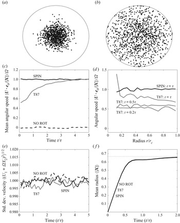
 $5\tau$. To set the scene figure 2(a,b) illustrates the dispersion of the ensemble in the SPIN model at early times (T87 and NO ROT appear statistically identical), showing the trajectories gradually filling the domain.
Panels (a,b): snapshot of  $10^3$ particles from the SPIN integration at
 $t=0.2\tau$ and
 $t=0.5\tau$, respectively. Panel (c): mean angular velocity. Panel (d): radial profile of angular velocity from T87 (
 $t=0.2,0.5$ and
 $1\;\tau$) and SPIN (
 $t=1\;\tau$). Panel (e): time evolution of the standard deviation of the
 $x$ component of the perturbation velocity in T87, SPIN and NO ROT simulations. Panel (f): time evolution of ensemble mean radius. Note that the three curves for T87, SPIN and NO ROT are indistinguishable. The dotted line shows the expected well-mixed value of
 $2/3$.

Figure 2(c) shows the key result, the ensemble mean angular speed of particles about the origin  $\langle \boldsymbol {U} \boldsymbol {\cdot } {\boldsymbol {e}}_\theta / |\boldsymbol {X}| \rangle$, as a function of time. Here
 ${\boldsymbol {e}}_\theta$ is the azimuthal unit vector. The ensemble average shown is calculated after first excluding those particles closest to the origin. This is because trajectories very close to the
 $z$-axis have a large variance in their azimuthal velocity which would prevent statistical convergence of the ensemble average. The excluded particles are those with a radius of less than one-tenth of the mean trajectory radius
 $\langle |\boldsymbol {X}| \rangle$. The key result is that trajectories in the SPIN model have mean angular speed
 $\varOmega$ from the beginning of the integration, as is clearly physical, whereas in the T87 model the initial angular speed is
 $\varOmega /2$. The T87 trajectories then spin-up on a time scale
 $\sim \tau$ to the correct angular speed.
Figure 2(d) shows snapshots of mean angular speed against radius at early times ( $t/\tau =0.2,0.5$ and
 $1$ in T87,
 $t/\tau =1$ in SPIN). Here the ensemble means are calculated by discarding trajectories according to their distance from the origin with a radial size of 0.05. Discarded trajectories close to the origin are subject to increasingly high variance. The results show that the spin-up of the angular speed in T87 appears to be somewhat faster for trajectories nearer to the origin. The radial profile of the angular speed in SPIN is, as is physical, independent of radius.
The insets (e,f) of figure 2 are included to show that the all three models are well mixed with identical dispersion in the radial direction. Figure 2(e) shows the standard deviation of the  $x$-direction component of the perturbation flow field. For all three models the standard deviation remains close to unity throughout the integration (to be well mixed requires only converge to unity at late times). Figure 2(f) shows the time evolution of the mean radius of trajectories
 $\langle | \boldsymbol {X} | \rangle$, which appears identical between the three models, and converges rapidly to the well-mixed value of
 $2/3$, corresponding to trajectories being uniformly distributed throughout the domain.
The simple isotropic homogeneous turbulent flow in solid-body rotation therefore demonstrates the major shortcoming of previous models, i.e. particles do not, on average, rotate at the rate of the mean flow. The spin model (in both weak and strong formulations) clearly rectifies this shortcoming, thereby demonstrating its value. The fact that the main correction term in the spin model has the form of a Coriolis acceleration could perhaps have been anticipated, and certainly adds physical understanding as to why it is the correct unique linear term to appear in all Lagrangian models of this type.
4.2. The weak spin model for turbulent channel flow
To understand the effects of other terms in the spin-model formulation it is necessary to consider turbulent flows with inhomogeneous statistics. A physically relevant and well-studied setting is that of turbulent channel flow, for which there exist theoretical and empirical experimentally verified profiles of the required turbulent statistics, from which the relevant trajectory models can be constructed. In order to be tractable these models will assume Gaussian single-point statistics, and are presented here in non-dimensional form, using the half-width  $h$ of the channel as the length scale and the friction velocity
 $u_*=(\tau _w/\rho )^{1/2}$ as the velocity scale, where
 $\tau _w$ is the shear stress at the wall and
 $\rho$ is the fluid density. Following convention, the unidirectional mean flow
 $\bar {\boldsymbol {u}}=\bar {u}(y)\boldsymbol {e}_x$ is directed along the
 $x$-axis, and
 $y$ is taken to be the across channel coordinate, so that the solid boundaries are located at
 $y=0,2$. All turbulent statistics depend only on the
 $y$-coordinate and
 \begin{equation}
\boldsymbol{\mathcal{C}} = \left( \begin{array}{@{}ccc@{}}
\sigma_1^2 & c_{12} & 0 \\ c_{12} &
~\sigma_2^2 & 0 \\ 0 & 0 & \sigma_3^2
\end{array} \right) \quad \text{and}\quad
\boldsymbol{\mathcal{B}}= \tfrac{1}{2} C_0 \epsilon
\boldsymbol{\mathcal{I}}.
\end{equation}
Reflecting boundary conditions are applied at the bounding surfaces  $y=0,2$.
Profiles of the mean velocity  $\bar {u}(y)$, the Reynolds stresses
 $\sigma _i(y)^2$,
 $c_{12}$ and the turbulent dissipation
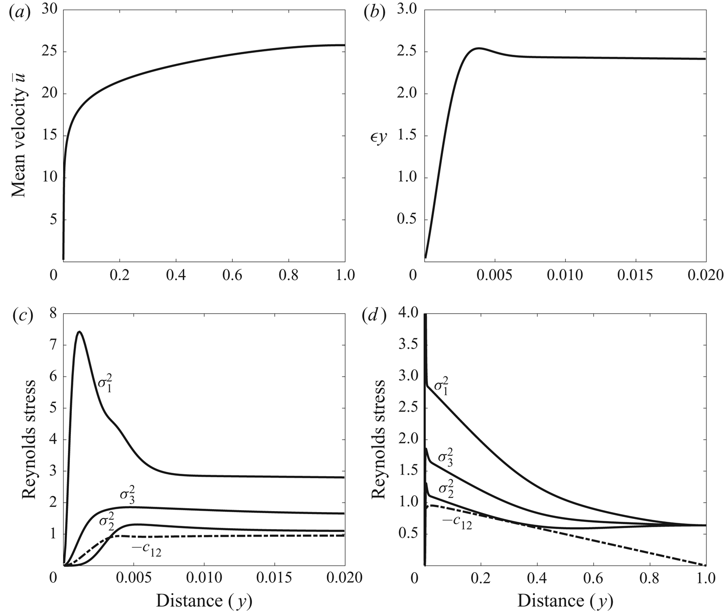
 $\epsilon (y)$ are shown in figure 3. Explicit analytical expressions are given in Appendix B. The profiles of figure 3 have been designed for a von Kármán number
 $h_+=u_*h/\nu =5000$, a value which is accessible in both experiments and direct numerical simulation, and the general principle behind their construction is that they give the correct behaviour in the log layer (
 $0.01 \lesssim y \lesssim 0.2$), which is the primary focus of the simulations discussed next. In non-dimensional variables, the log-layer behaviour is
 \begin{equation} \left. \begin{aligned} \bar{u} & \approx \frac{1}{\kappa} \log{(yh_+)}+B, \quad \epsilon \approx 2.45/y -1.7, \quad E_K \approx 3.2 \epsilon/ \bar{u}',\\ \sigma_1^2 & \approx 1.02 E_K, \quad \sigma_2^2 \approx 0.39 E_K, \quad \sigma_3^2 \approx 0.59 E_K, \quad c_{12} \approx{-}1. \end{aligned} \right\} \end{equation}
For the velocity profile,  $\kappa =0.39$ is the von Kármán constant, and
 $B=3.7$ the corresponding additive constant, recommended for channel flow by Nagib & Chauhan (Reference Nagib and Chauhan2008). For the turbulent dissipation
 $\epsilon$, the profile is based on the fit to direct-numerical-simulation data of Abe & Antonia (Reference Abe and Antonia2016, see their (4.26), and note that the units for
 $\epsilon$ here are
 $u_*^3h^{-1}$). The turbulent kinetic energy
 $E_K=(\sigma _1^2+\sigma _2^2+\sigma _3^2)/2$, is obtained from the observation that the normalised mean shear
 $\bar {u}'E_k/\epsilon$ is constant in the log layer (e.g. Pope Reference Pope2000, see their table 7.2 and figure 7.16), and the partitioning of
 $E_K$ between its directional components
 $\sigma _i^2$ is also uniform in the log layer and approximately satisfies the ratio
 $1.02:0.39:0.59$. Finally the vertical momentum flux
 $c_{12}$ is determined from the momentum balance equation, see Appendix B.
Profiles of various quantities in the  $h_+=5000$ turbulent channel flow. (a) Mean velocity profile
 $\bar {u}$. (b) Turbulent dissipation
 $\varepsilon$ multiplied by distance
 $y$ from wall in the near-wall region (cf. figure 8 of Abe & Antonia (Reference Abe and Antonia2016)). Dimensional units are
 $u_*^3$. (c) Reynolds stresses in the near-wall region (cf. figure 7.17 of Pope (Reference Pope2000)), dimensional units are
 $u_*^2$. (d) Reynolds stresses across the channel.

The weak spin model (3.41) and the T87 model (T87 (32), and also (2.10) above), for the perturbation velocities  $V_1=U_1-\bar {u}(Y)$,
 $V_2=U_2$ and
 $V_3=U_3$ each have the form
 \begin{equation} \textrm{d}V_i = \left( \bar{A}_i + \bar{B}_{ij} V_j + \bar{C}_{ijk} V_j V_k \right)\, \textrm{d}t + (C_0 \epsilon)^{1/2} \,\textrm{d}W_i,\quad i=1,2,3. \end{equation}
Note that the equations for  $V_1$ and
 $U_1$ are related by
 $\textrm {d}V_1=\textrm {d}U_1 - \bar {u}'(Y) U_2\, \textrm {d}t$. Explicit expressions for
 $\bar {A}_i$ and
 $\bar {C}_{ijk}$ are given in terms of the prescribed profiles
 $\sigma _i$,
 $c_{12}$,
 $\epsilon$, etc. in Appendix B. The important difference between the weak spin and T87 models will be shown later to be a result of the Coriolis term changing the linear term through changes in
 $\bar {B}_{ij}$. In T87
 \begin{equation} (\bar{B}_{ij})_{ T87}
={-}\frac{1}{2} C_0 \epsilon \left( \begin{array}{@{}ccc@{}}
\sigma^2_2 \varDelta^{{-}1} & -c_{12} \varDelta^{{-}1} & 0\\ -c_{12} \varDelta^{{-}1} & \sigma^2_1
\varDelta^{{-}1} & 0 \\ 0 & 0 & \sigma^{{-}2}_{3}
\end{array} \right), \end{equation}
where  $\varDelta =\sigma _1^2 \sigma _2^2 - c_{12}^2$, while in the weak spin model
 \begin{equation} (\bar{B}_{ij}) =
(\bar{B}_{ij})_{ T87} + \frac{1}{2} \left(
\begin{array}{@{}ccc@{}} 0 & \bar{u}' & 0 \\ -\bar{u}' & 0 & 0 \\
0 & 0 & 0 \end{array} \right).
\end{equation}
Equation (4.8) was integrated, in conjunction with the trajectory equations  $\textrm {d}X=(\bar {u}(Y)+V_1)\, \textrm {d}t$ and
 $\textrm {d}Y=V_2\, \textrm {d}t$, for the SPIN and T87 models and the results are presented in figure 4. (Dispersion in the
 $Z$ direction is uncoupled and is not simulated here). The integrations are for
 $N=5000$ trajectories, released at
 $(X(0),Y(0))=(0,0.05)$ and are relatively short (
 $t=2$, units are
 $h u_*^{-1}$) owing to stringent time-step requirements, because of the large near-wall gradients in the velocity and turbulence profiles. To obtain statistically convergent results, it was found that Euler–Maruyama time steps as small as
 $\delta t=10^{-7}$ are required close to the wall.
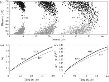
(a) Sample trajectories ( $10^3$) from the SPIN (black) and T87 (grey) simulations at
 $t=0.5$,
 $1$ and
 $1.6$. For clarity SPIN trajectories are reflected in the
 $y=1$ centreline. (b) Time evolution of mean trajectory cross-channel position
 $\langle Y \rangle$ for SPIN, MIX and T87 simulations. (c) Time evolution of standard deviation of trajectory cross-channel position
 $\langle (Y- \langle Y \rangle )^2 \rangle ^{1/2}$ for SPIN, MIX and T87 simulations.

Figure 4(a) shows snapshots of the first 1000 trajectories at  $t=0.5,1$ and
 $1.6$, with the position of the SPIN trajectories reflected in the
 $y=1$ centreline so that they appear in upper part of the channel. The main difference between the models is that cross-channel dispersion is enhanced in the SPIN model, as is seen more clearly in the lower panels where the ensemble mean and standard deviation of
 $Y$ are plotted against time. The dotted curve in these panels shows the results from a further simulation MIX, for which
 $\bar {B}_{ij}$ in (4.8) is equal to that of the SPIN model, while
 $\bar {A}_{i}$ and
 $\bar {C}_{ijk}$ are as for T87. The MIX results are statistically indistinguishable from the SPIN results, demonstrating that it is the change in
 $\bar {B}_{ij}$ (from (4.9) to (4.10)) which is key to the different behaviours.
The result that the cross-channel dispersion of particles is enhanced in the SPIN model appears to be in contradiction to the results of Borgas et al. (Reference Borgas, Flesch and Sawford1997) and Esler & Ramli (Reference Esler and Ramli2017), who have shown in certain settings that the additional rotational terms in (4.10) associated with the shear flow will act to suppress particle dispersion. To understand this result, the diffusive approximation (see e.g. Rodean Reference Rodean1996) to the model (4.8) is derived (in a slightly simplified setting) in Appendix B, see the result (B19). The component of the diffusion tensor  $\kappa _{22}$ controlling the cross-channel diffusivity is given in the two models by (B20). Inspection of (B20) reveals that, when the momentum flux
 $c_{12}$ is non-zero, it is possible for the rotational terms to increase the diffusivity
 $\kappa _{22}$, provided that
 $c_{12}$ and
 $\bar {u}'$ have opposite signs, as is always the case in channel flow. If the
 $c_{12}$ term is set to zero, as it is for example in Esler & Ramli (Reference Esler and Ramli2017), the rotational terms act to suppress the diffusivity as found in the previous studies. Calculations of
 $\kappa _{22}$ using (B20) for the turbulent channel flow considered here reveals that
 $\kappa _{22}$ is 7–10 % higher in the log-layer region in the SPIN model compared with T87, consistent with the enhanced dispersion seen in figure 4.
4.3. A simple isotropic Gaussian model of turbulence in a neutral atmospheric boundary layer
To supplement the results already discussed, simulations of an idealised atmospheric boundary-layer flow have also been performed. The set-up is that studied in Esler & Ramli (Reference Esler and Ramli2017), with a mean velocity  $\bar {\boldsymbol {u}}=\bar {u}(z)\boldsymbol {e}_x$, i.e. a steady unidirectional shear flow, and shares many features with state-of-the-art atmospheric dispersion models, such as FLEXPART (Stohl et al. Reference Stohl, Forster, Frank, Seibert and Wotawa2005) which are designed primarily to study dispersion in the region above the log layer. For example, FLEXPART omits off-diagonal terms in
 $\boldsymbol {\mathcal {C}}$, and the velocity field is supplied by the meteorology. Here, to further simplify matters, the turbulent statistics are taken to be isotropic, and depend only on the
 $z$ coordinate, so that
 \begin{equation} \boldsymbol{\mathcal{C}} = \sigma(z)^2 \, \boldsymbol{\mathcal{I}} \quad \text{and}\quad \boldsymbol{\mathcal{B}}= \frac{\sigma(z)^2}{\tau(z)} \, \boldsymbol{\mathcal{I}}. \end{equation}
Trajectories are reflected at the surface and at the top of the boundary layer (modelling the effect of a jump in stratification). The simpler set-up allows the SPIN and T87 models to be integrated until particles are well-mixed in the vertical, and for the long-time horizontal dispersion of particles to be studied.
The weak spin model (3.41) for this set-up is
 \begin{align} \left. \begin{aligned} \textrm{d}V_1 & = \left( -\frac{V_1}{\tau} +\frac{1}{2} \bar{u}' V_3 +\frac{2}{3} V_1 V_3 \frac{\sigma'}{\sigma} \right) \textrm{d}t + \left( \frac{2 \sigma^2}{\tau} \right)^{1/2}\, \textrm{d}W_1, \\ \textrm{d}V_2 & = \left( -\frac{V_2}{\tau} +\frac{2}{3} V_2 V_3 \frac{\sigma'}{\sigma}\right) \textrm{d}t + \left( \frac{2 \sigma^2}{\tau} \right)^{1/2} \,\textrm{d}W_2, \\ \textrm{d}V_3 & = \left( -\frac{V_3}{\tau} -\frac{1}{2} \bar{u}' V_1 + \frac{1}{3} \left( V_1^2+V_2^2 + 3V_3^2 +\sigma^2 \right) \frac{\sigma'}{\sigma} \right) \textrm{d}t + \left( \frac{2 \sigma^2}{\tau} \right)^{1/2} \,\textrm{d}W_3, \end{aligned} \right\} \end{align}
where  $V_1=U_1-\bar {u}(Z)$,
 $V_2=U_2$ and
 $V_3=U_3$ are the components of the perturbation velocity, and it is understood that
 $\sigma$,
 $\sigma '$,
 $\tau$ and
 $\bar {u}'$ are evaluated at
 $z=Z$, i.e.
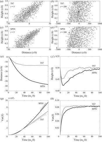
 $\sigma \equiv \sigma (Z)$, etc. A notable feature of (4.12) in this setting is that all three velocity equations are coupled, in contrast to the T87 equations, in which vertical dispersion (for example) can be considered in isolation.
The corresponding T87 model is
 \begin{equation} \left. \begin{aligned} \textrm{d}V_1 & = \left( -\frac{V_1}{\tau} + V_1 V_3 \frac{\sigma'}{\sigma} \right) \textrm{d}t + \left( \frac{2 \sigma^2}{\tau} \right)^{1/2} \,\textrm{d}W_1,\\ \textrm{d}V_2 & = \left( -\frac{V_2}{\tau} + V_2 V_3 \frac{\sigma'}{\sigma}\right) \textrm{d}t + \left( \frac{2 \sigma^2}{\tau} \right)^{1/2}\, \textrm{d}W_2,\\ \textrm{d}V_3 & = \left( -\frac{V_3}{\tau} + \left( V_3^2+\sigma^2 \right) \frac{\sigma'}{\sigma} \right) \textrm{d}t + \left( \frac{2 \sigma^2}{\tau} \right)^{1/2} \textrm{d}W_3. \end{aligned} \right\} \end{equation}
Both the SPIN and T87 models are integrated together with the trajectory equations  $\textrm {d}X=(V_1+\bar {u}(Z)) \,\textrm {d}t$ and
 $\textrm {d}Z=V_3\,\textrm {d}t$ (dispersion in the horizontal cross-stream direction is uncoupled and is not simulated here). The profiles of
 $\bar {u}(z)$,
 $\sigma (z)$ and
 $\tau (z)$ are chosen following Esler & Ramli (Reference Esler and Ramli2017):
 \begin{equation} \left. \begin{aligned} \bar{u}(z) & = \varGamma_s (z-\tfrac{1}{2} ), \\ \sigma(z) & = 1.3 \exp{({-}2 \hat{z}/z_n)}, \\ \tau(z) & = \frac{\hat{z} \exp{(2 \hat{z}/z_n)}}{2.6(1+15\hat{z}/z_n)}, \end{aligned} \right\} \end{equation}
where distance is non-dimensionalised by the boundary-layer height  $h$, velocity by the friction velocity
 $u_*$ and time by
 $hu_*^{-1}$. The profiles for
 $\sigma$ and
 $\tau$ are chosen to be typical of a neutral atmospheric boundary layer. Here
 $z_n=0.8$ and
 $\hat {z}=z_b+z(1-2z_b)$ is a rescaled height used to regularise the profiles (with
 $z_b=0.05$), see Esler & Ramli (Reference Esler and Ramli2017) for discussion. The mean wind profile
 $\bar {u}(z)$ is chosen to be a linear shear for simplicity, with the non-dimensional parameter
 $\varGamma _s=(u_{ top}-u_{ surf})/u_*$ given by the ratio of the wind increase across the boundary layer to the friction velocity. A value
 $\varGamma _s = 20$ is used, which is at the upper end of observed values.
The models ACW and CW used to generate the rapidly rotating trajectories shown in figure 1 in the introduction are the T87 model (4.13) augmented by the additional acceleration  $\boldsymbol {a}_+=\varGamma (V_3,0,-V_1)^{\textrm {T}}$. For the ACW model
 $\varGamma =-50$ and for the CW model
 $\varGamma =50$ (dimensional units
 $h u_*^{-1}$). Notice that the choice
 $\varGamma =\varGamma _s/2$ in
 $\boldsymbol {a}_+$ recovers the linear term in the SPIN model, which shows that the SPIN model has a trajectory rotation rate which, compared with T87, is significantly biased towards the CW model when
 $\varGamma _s$ is large. This outcome is intuitive because the linear shear in (4.14) evidently has a clockwise rotating component.
Figure 5 compares ensembles of  $10^4$ trajectories in the SPIN and T87 models. The particles are released at
 $t=0$ from
 $(X(0),Z(0))=(0,0.5)$, with velocities drawn from
 $p_f$, and are followed for time
 $100hu_*^{-1}$. Figure 5(a,b), which shows a snapshot of particles at an early time (
 $t=5hu_*^{-1}$), shows that the vertical diffusion of particles is significantly suppressed in the SPIN model, as is expected from (B20) when
 $c_{12}$ is neglected. Owing to the Taylor dispersion mechanism (Taylor Reference Taylor1953; Saffman Reference Saffman1962; Esler & Ramli Reference Esler and Ramli2017), it follows that effective horizontal diffusion will be enhanced in the SPIN model at late times, and this is indeed what is seen in the later snapshots in figure 5(c,d) (
 $t=100hu_*^{-1}$). Figure 5(e,f) show the evolution of the ensemble mean location,
 $\langle X \rangle$ and
 $\langle Z \rangle$, respectively. In both models there is an initial bias for trajectories to move towards the surface, and, because they then experience negative mean winds on average, to head leftwards. The effect is significantly stronger in SPIN compared with T87, with the final ensemble mean position, which becomes stationary once the particles are well-mixed, ending up around four-times farther leftwards from the release point in SPIN compared with T87. It is also notable in figure 5(f) that, owing to the suppressed vertical diffusivity, SPIN is seen to take significantly longer to reach a well-mixed state (in which
 $\langle Z \rangle =0.5$) compared with T87.
Panels (a,b): snapshot of  $10^3$ particles from the T87 and SPIN boundary-layer integrations at
 $t=5hu_*^{-1}$. The cross shows the point of release and the filled black circle the ensemble mean position. Panels (c,d): as for panels (a,b), but for
 $t=100hu_*^{-1}$ (note the change in horizontal scale). Panel (e): time evolution of
 $\langle X \rangle$ in the T87 and SPIN runs. Panel (f): time evolution of
 $\langle Z \rangle$. The dotted line shows the well-mixed value
 $(={1}/{2})$. Panel (g): time evolution of Var
 $(X)$. Panel (h): time evolution of Var
 $(Z)$. The dotted line shows the well-mixed value
 $(={1}/{12})$.

Figure 5(g) shows the rate of increase of Var $(X)$ in each model, showing that the rate of horizontal dispersion remains comparable until around
 $t=40hu_*^{-1}$, after which it is significantly greater in the SPIN model. At late times it is natural to define an effective horizontal diffusivity
 \begin{equation} \kappa_{ eff}= \lim_{t \to \infty} \frac{\mbox{Var}(X)}{2t}. \end{equation}
Building on the work of Saffman (Reference Saffman1962), the question of how to determine  $\kappa _{ eff}$, by exploiting the diffusive limit of the random flight model (1.1), was addressed by Esler & Ramli (Reference Esler and Ramli2017, see their § 3.4). The key results in the current context are that, for the T87 model (4.13) at leading order,
 \begin{equation} \kappa_{ eff} = \left[ \frac{F^2}{\sigma^2 \tau} + \sigma^2 \tau \right], \quad \text{(T87)}, \end{equation}
where  $F(z)=\int _0^z \bar {u}(z') \, \textrm {d}z'$, and the square brackets denote a vertical average. For comparison (see (37) of Esler & Ramli Reference Esler and Ramli2017), when the linear terms in the SPIN model are added then
 \begin{equation} \kappa_{ eff} = \left[ \frac{\hat{F}^2}{\varPi \sigma^2 \tau} + \varPi \sigma^2 \tau \right],\quad \text{(SPIN)}, \end{equation}
where  $\varPi (z)=1/(1+\bar {u}'^2 \tau ^2/4)$ and
 \begin{equation} \hat{F}(z)=F(z)+\varPi(z) \sigma(z)^2 \tau(z)^2 \bar{u}'(z)/2- \varPi(0) \sigma(0)^2 \tau(0)^2 \bar{u}'(0)/2. \end{equation}
The effective diffusivities in (4.16) and (4.17) are straightforward to evaluate, and give a good fit to the calculations, see the dotted lines on figure 5(g). (The apparent overestimate of the slope for the SPIN model is due to the SPIN ensemble not being completely well-mixed by  $t=100$
 $hu_*^{-1}$. Calculations from a longer SPIN run (
 $200 h u_*^{-1}$) confirm the accuracy of (4.17) at late times, in fact (4.17) slightly underestimates (
 $\sim 4\,\%$) the calculated late time
 $\kappa _{ eff}$.) The difference between the predictions is due to the factor
 $\varPi \le 1$ acting to increase the dominant first term in (4.17) relative to that of (4.16) (the change
 $F \to \hat {F}$ is negligible by comparison), thereby increasing
 $\kappa _{ eff}$. In the scenario of figure 5, the linear terms in the SPIN model increase
 $\kappa _{ eff}$ by 83 % (from
 $\kappa _{ eff} \approx 405\,u_*h$ to
 $742\,u_*h$) for the current simulations relative to the T87 value. It is important to note that the large difference between SPIN and T87 is for a relatively large value of the shear parameter (
 $\varGamma _s=20$), and for lower values (e.g
 $\varGamma _s=5$ used in Esler & Ramli Reference Esler and Ramli2017)) the increase in
 $\kappa _{ eff}$ is much less significant.
Finally figure 5(h) serves to confirm that both SPIN and T87 models are indeed converging towards a well-mixed state, by verifying that  $\text {Var}(Z)$ in each model asymptotes towards the well-mixed value of
 $1/12$.
The important message from figure 5 is that correcting Lagrangian models to account for the spin condition will lead to significant changes in trajectory behaviour in atmospheric boundary-layer modelling. In this atmospheric boundary-layer setting, the SPIN model is subject to lower vertical diffusivity and, as a consequence, higher long-time effective horizontal diffusivity owing to the shear dispersion mechanism. The key parameter in this respect is the shear parameter  $\varGamma _s$ which, for the SPIN terms to make a difference, needs to be large enough for
 $\varPi (z)$ to be significantly less than one throughout much of the boundary layer.
5. Conclusions
The question of how to formulate a unique Lagrangian particle dispersion model which is physically consistent with the prescribed statistics of an inhomogeneous turbulent flow has been studied since the seminal work of T87. Here a comprehensive solution has been presented, underpinned by the key physical requirement of rotational invariance; if a homogeneous isotropic turbulent flow is put into solid-body rotation with angular velocity  $\boldsymbol {\varOmega }$, then the expected rotation rate of particle trajectories in that flow should also be
 $\boldsymbol {\varOmega }$. The spin condition (3.13) enforces this rotational invariance, by ensuring that particles experience a Coriolis acceleration
 $\boldsymbol {a}_r= 2 \boldsymbol {\varOmega } \times \boldsymbol {v}$ in the solid-body rotation flow, which generalises to
 $\boldsymbol {a}_r= \bar {\boldsymbol {\omega }} \times \boldsymbol {v}$ in flows with inhomogeneous mean vorticity
 $\bar {\boldsymbol {\omega }}$. Here
 $\boldsymbol {a}_r$ is the component of the particle acceleration
 $\boldsymbol {a}$ which is antisymmetric and linear in the perturbation velocity
 $\boldsymbol {v}$.
The spin condition, taken together with the T87 well-mixed condition, uniquely specifies the acceleration  $\boldsymbol {a}$. The strong form (3.13), however, leads to models (in general (3.16)–(3.21) for the canonical case (3.27)) which are not only complicated to express but also have the property that
 $\boldsymbol {a}$ grows exponentially with
 $|\boldsymbol {v}|$. It seems that these undesirable features arise because it is too much to expect a trajectory model to be well-mixed, obey the strong spin condition, and have only local dependence on the mean velocity and turbulent statistics. After all, in the Navier–Stokes equations themselves, the relationship between the distribution of accelerations
 $\boldsymbol {a}$ experienced by a single particle in an ensemble of flows will necessarily have a non-local dependence on the velocity statistics (because, for example, the instantaneous pressure field depends non-locally and nonlinearly on the velocity distribution through the solution of an elliptic equation). In order to meet the artificial constraint of locality, it seems models must either break the spin condition, or they will require large accelerations which are probably unphysical. Further evidence that the strong spin models are overconstrained comes from the fact that the ensemble mean acceleration
 $\bar {\boldsymbol {a}}$ in the canonical strong spin model differs from the correct Navier–Stokes value (3.42).
The weak spin condition (3.14), therefore, constitutes a reasonable compromise in which some degrees of rotational freedom are retained to counterbalance the constraints introduced by locality, but the correct mean spin rate is retained. It is particularly appealing that the weak spin condition leads to the unique quadratic well-mixed weak spin model (3.41). As seen in § 4, the differences between the weak spin model and T87 appear to be large enough to make a significant quantitative difference to particle dispersion in at least some experimental or observational settings, and it is to be hoped that future experimental work will be able to benchmark its performance.
Finally, it is worth returning briefly to the question of what the implications of the spin condition are for the turbulence-modelling approach reviewed in Pope (Reference Pope1994). In the absence of the powerful constraint, used in the T87 approach, of completely specifying the turbulent statistics, the spin condition will become just an additional constraint on the antisymmetric components of the undetermined tensor (e.g.  $\mathcal {G}_{ij}$ in (52) of Pope (Reference Pope1994)) in the GLM. A topic of future study will be whether this additional constraint can be used effectively to narrow the range of acceptable the GLM. Additionally, only single particle dispersion has been considered here. Pair dispersion models (e.g. Sawford Reference Sawford2001) have their own well-mixed conditions and non-uniqueness problems to which the present approach might also be applied.
Declaration of interests
The author reports no conflict of interest.
Appendix A. Calculation of  $\bar {\boldsymbol {a}}$ in the strong spin canonical model

Here the result (3.26), which is necessary to constrain the strong spin canonical model, is obtained. In general the result is found using the consistency constraint (3.17) to calculate the velocity-space mean of the acceleration  $\bar {\boldsymbol {a}}$. For the example of the canonical model, detailed in § 3.3, the situation is complicated by the fact that the integral defining (3.17) does not converge. The required result for
 $\bar {\boldsymbol {a}}$ can nevertheless be found by interpreting the integral constraint in the following principal value sense:
 $$\begin{gather} \bar{ \chi p_f^{{-}1} \boldsymbol{v} } \equiv \lim_{R \to \infty} \int_{\varOmega_R} \left( \left( \frac{\boldsymbol{v} \boldsymbol{\cdot} \boldsymbol{\mathcal{A}} \boldsymbol{\cdot} \boldsymbol{v}}{\boldsymbol{v} \boldsymbol{\cdot} \boldsymbol{\mathcal{C}}^{{-}1} \boldsymbol{\cdot} \boldsymbol{v} } - \frac{\boldsymbol{\mathcal{A}} : \boldsymbol{\mathcal{C}}}{3} \right) P( \boldsymbol{v} \boldsymbol{\cdot} \boldsymbol{\mathcal{C}}^{{-}1} \boldsymbol{\cdot} \boldsymbol{v} ) - \frac{\boldsymbol{v} \boldsymbol{\cdot} \boldsymbol{\mathcal{A}} \boldsymbol{\cdot} \boldsymbol{v}}{\boldsymbol{v} \boldsymbol{\cdot} \boldsymbol{\mathcal{C}}^{{-}1} \boldsymbol{\cdot} \boldsymbol{v} }\right.\nonumber\\ \left.+\left( \frac{\boldsymbol{v} \boldsymbol{\cdot} \mathcal{G} : \boldsymbol{v} \boldsymbol{v}}{\boldsymbol{v} \boldsymbol{\cdot} \boldsymbol{\mathcal{C}}^{{-}1} \boldsymbol{\cdot} \boldsymbol{v} } - \frac{ \boldsymbol{v}\boldsymbol{\cdot} \boldsymbol{g}}{4} \right) Q( \boldsymbol{v} \boldsymbol{\cdot} \boldsymbol{\mathcal{C}}^{{-}1} \boldsymbol{\cdot} \boldsymbol{v} ) - \frac{\boldsymbol{v} \boldsymbol{\cdot} \mathcal{G} : \boldsymbol{v} \boldsymbol{v}}{\boldsymbol{v} \boldsymbol{\cdot} \boldsymbol{\mathcal{C}}^{{-}1} \boldsymbol{\cdot} \boldsymbol{v} } \right)\, \boldsymbol{v} \, p_f \, \textrm{d}\boldsymbol{v}=0, \end{gather}$$
where  $\varOmega _R=\{ \boldsymbol {v} \; : \; \boldsymbol {v} \boldsymbol {\cdot } \boldsymbol {\mathcal {C}}^{-1} \boldsymbol {\cdot } \boldsymbol {v}< R^2\}$ is an ellipsoidal subset of velocity space with volume proportional to
 $R^3$, and the rest of the notation is as detailed in § 3.3.
Consider first the integral condition above applied on  $\varOmega _R$ when
 $R$ is finite. Changing variables by writing
 $\boldsymbol {v} = \boldsymbol {\mathcal {C}}^{1/2} \boldsymbol {\cdot } \boldsymbol {w}$, where
 $\boldsymbol {\mathcal {C}}^{1/2}$ denotes the matrix square root of
 $\boldsymbol {\mathcal {C}}$, the condition simplifies to
 \begin{align} \int_{|\boldsymbol{w}|< R} \left( \left( \frac{\boldsymbol{w} \boldsymbol{\cdot} \mathcal{H} : \boldsymbol{w} \boldsymbol{w}}{w^2} - \frac{ \boldsymbol{w} \boldsymbol{\cdot} \boldsymbol{\mathcal{C}}^{1/2} \boldsymbol{\cdot} \boldsymbol{g}}{4} \right) Q( w^2 ) - \frac{\boldsymbol{w} \boldsymbol{\cdot} \mathcal{H} : \boldsymbol{w} \boldsymbol{w}}{w^2 } \right) (\boldsymbol{\mathcal{C}}^{1/2} \boldsymbol{\cdot} \boldsymbol{w}) \textrm{e}^{{-}w^2/2} \, \textrm{d}\boldsymbol{w}=0, \end{align}
where  $\mathcal {H}$ has components
 $H_{ijk}=G_{mpq}D_{mi}D_{pj}D_{qk}$, where
 $D_{ij}$ are the entries of
 $\boldsymbol {\mathcal {C}}^{1/2}$, and
 $w=|\boldsymbol {w}|$. The corresponding terms involving
 $P(\boldsymbol {\cdot })$ vanish because their integral contains only odd powers of
 $\boldsymbol {w}$. Next, the following results can be applied, which are valid in three dimensions for any function
 $f(w)$ of the radial coordinate
 $w$, and can be easily verified by expressing the integrals in spherical polar coordinates:
 $$\begin{gather} \int_{|\boldsymbol{w}|< R} w_i w_j f(w) \, \textrm{d}\boldsymbol{w} = \frac{4{\rm \pi}}{3} \, \delta_{ij} \, \int_0^R w^4 f(w) \, \textrm{d}w, \end{gather}$$
 $$\begin{gather}\int_{|\boldsymbol{w}|< R} w_i w_j w_k w_l f(w) \, \textrm{d}\boldsymbol{w} = \frac{4{\rm \pi}}{15} \left(\delta_{ij} \delta_{kl} + \delta_{ik} \delta_{jl}+ \delta_{il} \delta_{jk} \right) \int_0^R w^6 f(w) \, \textrm{d}w. \end{gather}$$
Applying these results to the integral condition it is found, after exploiting the symmetry  $G_{ijk}=G_{ikj}$, that
 \begin{equation} \frac{4{\rm \pi}}{15} \left( 2 \boldsymbol{\mathcal{C}} : \mathcal{G} \boldsymbol{\cdot} \boldsymbol{\mathcal{C}} + \boldsymbol{\mathcal{C}} \boldsymbol{\cdot} \mathcal{G} : \boldsymbol{\mathcal{C}} \right) (I_R-J_R) + \frac{\rm \pi}{3} \boldsymbol{\mathcal{C}} \boldsymbol{\cdot} \boldsymbol{g} I_R =0, \end{equation}
where
 \begin{align} I_R & = \int_0^R w^4 Q(w^2) \textrm{e}^{{-}w^2/2} \, \textrm{d}w= 8 R +4R \textrm{e}^{{-}R^2/2} -6\sqrt{2{\rm \pi}}\; \textrm{erf}(R/\sqrt{2}) \end{align}
 \begin{align} \text{and}\quad J_R & = \int_0^R w^4 \textrm{e}^{{-}w^2/2} \, \textrm{d}w= \tfrac{3}{2} \sqrt{2{\rm \pi}}\; \textrm{erf}(R/\sqrt{2})-R (R^2+3)\textrm{e}^{{-}R^2/2}. \end{align}
Inserting for  $\mathcal {G}$ and
 $\boldsymbol {g}$, and rearranging gives
 \begin{align} \bar{\boldsymbol{a}}= (\partial_t + \bar{\boldsymbol{u}} \boldsymbol{\cdot} \boldsymbol{\nabla} ) \bar{\boldsymbol{u}} + \tfrac{4}{5} \boldsymbol{\nabla} \boldsymbol{\cdot} \boldsymbol{\mathcal{C}} + \tfrac{1}{10} \boldsymbol{\mathcal{C}} \boldsymbol{\cdot} \boldsymbol{\nabla} \boldsymbol{\mathcal{C}}^{{-}1} : \boldsymbol{\mathcal{C}} - \tfrac{4}{5} (J_R/I_R) \left( \boldsymbol{\nabla} \boldsymbol{\cdot} \boldsymbol{\mathcal{C}} - \tfrac{1}{2} \boldsymbol{\mathcal{C}} \boldsymbol{\cdot} \boldsymbol{\nabla} \boldsymbol{\mathcal{C}}^{{-}1} : \boldsymbol{\mathcal{C}} \right). \end{align}
Taking the limit  $R\to \infty$, in which
 $J_R/I_R \to 0$, the result (3.26) is obtained.
Appendix B. Turbulent channel flow: complete description of the weak spin and T87 models
In this appendix, full details of the set-up and implementation of the turbulent channel-flow simulations of § 4.2 are presented. First, the complete equations for the velocity, Reynolds stresses and turbulent dissipation profiles are
 $$\begin{gather} \bar{u}(y) = I_0(y)\left( y h_+{-}0.1\left(yh_+\right)^2\right) +(1-I_0(y))\left(\frac{1}{\kappa}\log{\left(yh_+ \right)}+B+\frac{2\varPi}{\kappa}W(y)\right), \end{gather}$$
 $$\begin{gather}\sigma_1(y) = I_1(y) \left( 3 \tanh{(0.37 yh_+)} \right) + (1-I_1(y)-\bar{I}(y))\sqrt{1.02} f_{ log}(y) + 0.8 \bar{I}(y), \end{gather}$$
 $$\begin{gather}\sigma_2(y) = I_2(y) \left( 1.2 \tanh{(0.004 (yh_+)^2)} \right)+ (1-I_2(y)-\bar{I}(y))\sqrt{0.39} f_{ log}(y) + 0.8 \bar{I}(y), \end{gather}$$
 $$\begin{gather}\sigma_3(y) = I_3(y)\left( 1.4 \tanh{(0.14 yh_+)} \right) + (1-I_3(y)-\bar{I}(y))\sqrt{0.59} f_{ log}(y) + 0.8 \bar{I}(y), \end{gather}$$
 $$\begin{gather}c_{12}(y) ={-}(1-y-h_+ \bar{u}'), \end{gather}$$
 $$\begin{gather}\epsilon(y) = I_4(y)\left( \frac{h_+}{6} \right)+ (1-I_4(y))\left( \frac{2.45}{y}-1.7 \right), \end{gather}$$
 $$\begin{gather}f_{ log}(y) = \left( \frac{3.2 \epsilon}{\bar{u}'+1} \left( 1- \bar{I}(y) \right) + 1.2\bar{I}(y) \right)^{1/2}. \end{gather}$$
Here  $W(y)$ is the wake function for channel flow given by (12) of Nagib & Chauhan (Reference Nagib and Chauhan2008), and
 $\varPi =0.05$. The functions
 $I_i(y)=\exp {(-y^2/2s_i^2)}$ and
 $\bar {I}(y)=\exp {(-(1-y)^2/2\bar {s}^2)}$ are interpolation functions which allow for smooth transition between the regions (
 $s_i=\{5, 13, 30, 40, 9.5 \}/h_+$ for
 $i=0,4$ and
 $\bar {s}=0.4$). As discussed in the main text, these profiles are designed to give the correct values (4.7) in the log-layer region, and to interpolate smoothly to physically reasonable profiles in the outer region near the channel centre, and the inner region near the wall. The different coefficients appearing in the interpolating functions have been chosen with a view to obtaining approximately the correct behaviour in the overlap between the inner and log-layer regions (see e.g. panels (b) and (c) of figure 3).
Next, explicit expressions for  $\bar {A}_i$ and
 $\bar {C}_{ijk}$ in (4.8) are presented for the weak spin model (3.41) and T87 model (2.10), for ease of implementation of these models. The remaining terms
 $\bar {B}_{ij}$ are given by (4.9) and (4.10), respectively. First, the vectors
 $\bar {A}_i$ are given by
 \begin{equation} (\bar{A}_{i}) =
\tfrac{2}{3} \left( \begin{array}{@{}c@{}} c_{12}'-\tfrac{1}{4}
c_{12} D'/D \\ (\sigma_2^2)'-\tfrac{1}{4} \sigma_2^2
D'/D \\ 0 \end{array} \right) \quad (\bar{A}_{i})_{T87}
= \tfrac{1}{2} \left( \begin{array}{@{}c@{}} c_{12}' \\
(\sigma_2^2)' \\ 0 \end{array} \right), \end{equation}
where  $D=|\boldsymbol {\mathcal {C}}|=(\sigma _1^2 \sigma _2^2 - c_{12}^2) \sigma _3^2$. Then, defining
 $\varDelta =\sigma _1^2 \sigma _2^2 -c_{12}^2$,
 \begin{align} (\bar{C}_{1jk}) &=
\frac{1}{6} \left( \begin{array}{@{}ccc@{}}
-c_{12}\left(\dfrac{\sigma_2^2}{\varDelta}\right)' &
\dfrac{(\sigma_1^2)'\sigma_2^2 -c_{12}c_{12}'}{\varDelta}
+c_{12}\left(\dfrac{c_{12}}{\varDelta}\right)' & 0 \\
\dfrac{(\sigma_1^2)'\sigma_2^2 -c_{12}c_{12}'}{\varDelta}
+c_{12}\left(\dfrac{c_{12}}{\varDelta}\right)' &
\dfrac{2c_{12}'\sigma_1^2 -2(\sigma_1^2)'
c_{12}}{\varDelta}
-c_{12}\left(\dfrac{\sigma_1^2}{\varDelta}\right)' & 0 \\0
& 0 & -c_{12} (\sigma_3^{{-}2})' \end{array}
\right), \end{align}
 \begin{align} (\bar{C}_{2jk}) & =
\frac{1}{6} \left( \begin{array}{@{}ccc@{}}
-\sigma_2^2\left(\dfrac{\sigma_2^2}{\varDelta}\right)' &
\dfrac{c_{12}' \sigma_2^2 -c_{12}(\sigma_2^2)'}{\varDelta}
+\sigma_2^2\left(\dfrac{c_{12}}{\varDelta}\right)' & 0 \\
\dfrac{c_{12}'\sigma_2^2 -c_{12}(\sigma_2^2)'}{\varDelta}
+\sigma_2^2\left(\dfrac{c_{12}}{\varDelta}\right)' &
\dfrac{2(\sigma_2^2)'\sigma_1^2 -2c_{12}'
c_{12}}{\varDelta}
-\sigma_2^2\left(\dfrac{\sigma_1^2}{\varDelta}\right)' & 0
\\0 & 0 & -\sigma_2^2 (\sigma_3^{{-}2})'
\end{array} \right),
\end{align}
 \begin{align} (\bar{C}_{3jk}) & =
\frac{1}{6} \left( \begin{array}{@{}ccc@{}} 0 & 0 & 0 \\ 0 & 0 &
\dfrac{(\sigma_3^2)'}{\sigma_3^2} \\ 0 &
\dfrac{(\sigma_3^2)'}{\sigma_3^2} & 0 \end{array}
\right), \end{align}
whereas, for T87
 \begin{gather} (\bar{C}_{1jk})_{T87} = \frac{1}{4} \left( \begin{array}{ccc} 0 & \dfrac{(\sigma_1^2)'\sigma_2^2 -c_{12}c_{12}'}{\varDelta} & 0 \\ \dfrac{(\sigma_1^2)'\sigma_2^2 -c_{12}c_{12}'}{\varDelta} & \dfrac{2c_{12}'\sigma_1^2 -2(\sigma_1^2)' c_{12}}{\varDelta} & 0 \\0 & 0 & 0 \end{array} \right), \end{gather}
 \begin{gather} (\bar{C}_{2jk})_{T87} = \frac{1}{4} \left( \begin{array}{ccc} 0 & \dfrac{c_{12}' \sigma_2^2 -c_{12}(\sigma_2^2)'}{\varDelta} & 0 \\ \dfrac{c_{12}'\sigma_2^2 -c_{12}(\sigma_2^2)'}{\varDelta} & \dfrac{2(\sigma_2^2)'\sigma_1^2 -2c_{12}' c_{12}}{\varDelta} & 0 \\0 & 0 & 0 \end{array} \right), \end{gather}
 \begin{gather} (\bar{C}_{3jk})_{T87} = \frac{1}{4} \left( \begin{array}{ccc} 0 & 0 & 0 \\ 0 & 0 & \dfrac{(\sigma_3^2)'}{\sigma_3^2} \\0 & {(\sigma_3^2)'}/{\sigma_3^2} & 0 \end{array} \right). \end{gather}
These formulas complete the full specification of the T87 and SPIN models given by (4.8) in § 4.2.
B.1. Diffusive limit of (4.8)
Consider (4.8) with  $\bar {A}_i = \bar {C}_{ijk}=0$ and with
 $\bar {B}_{ij}$ and
 $\epsilon$ constant, together with the accompanying trajectory equation
 \begin{equation} \left. \begin{aligned} \textrm{d}V_i & = \bar{B}_{ij} V_j \textrm{d}t + (C_0 \epsilon)^{1/2} \,\textrm{d}W_i,\quad i=1,2,3, \\ \textrm{d}X_i & = \left( V_j + \bar{u}( \boldsymbol{X}) \right) \,\textrm{d}t. \end{aligned} \right\} \end{equation}
The Fokker–Planck equation for this system can be written
 \begin{equation} \delta^2 \left( p_t + (\bar{\boldsymbol{u}} \boldsymbol{\cdot} \boldsymbol{\nabla}) p \right) + \delta ( \boldsymbol{v} \boldsymbol{\cdot} \boldsymbol{\nabla}) p + \boldsymbol{\nabla}_{\boldsymbol{v}} \boldsymbol{\cdot} \left( (\bar{\boldsymbol{\mathcal{B}}} \boldsymbol{\cdot} \boldsymbol{v} ) p - \tfrac{1}{2} C_0 \epsilon \boldsymbol{\nabla}_{\boldsymbol{v}} p \right)= 0, \end{equation}
with the parameter  $\delta$ set equal to one. To obtain the diffusive approximation to (B15) it is necessary to rescale time, space and mean velocity variables so that
 $\delta \ll 1$ becomes a small parameter, a process which can be formally justified in flows where a clear separation of scales can be maintained. See Esler & Ramli (Reference Esler and Ramli2017) for a more formal treatment and discussion. Then, seeking an asymptotic solution
 $p=p_0 + \delta p_1 + \delta ^2 p_2 +\cdots$ leads to the hierarchy of equations
 \begin{equation} \left. \begin{aligned} \mathcal{L}p_0 & = 0, \\ \mathcal{L}p_1 & ={-} ( \boldsymbol{v} \boldsymbol{\cdot} \boldsymbol{\nabla}) p_0, \\ \mathcal{L}p_2 & ={-} ( \boldsymbol{v} \boldsymbol{\cdot} \boldsymbol{\nabla}) p_1 - \left( p_t + (\bar{\boldsymbol{u}} \boldsymbol{\cdot} \boldsymbol{\nabla}) p_0, \right) \\ & \vdots \end{aligned} \right\} \end{equation}
where  $\mathcal {L}p \equiv \boldsymbol {\nabla }_{\boldsymbol {v}} \boldsymbol {\cdot } ( (\bar {\boldsymbol {\mathcal {B}}} \boldsymbol {\cdot } \boldsymbol {v} ) p - (C_0 \epsilon \boldsymbol {\nabla }_{\boldsymbol {v}} p)/2 )$ denotes the linear operator in the first equation. The solution to the first equation is the well-mixed solution
 $p_0=c(\boldsymbol {x},t)p_f$, where
 $p_f$ is given by (2.9) with
 $\boldsymbol {\mathcal {C}}^{-1} =- (\bar {\boldsymbol {\mathcal {B}}}+ \bar {\boldsymbol {\mathcal {B}}}^{\textrm {T}})/(C_0 \epsilon )$ and where
 $c(\boldsymbol {x},t)$ is at this stage an undetermined concentration field. A particular integral solution to the second equation is then found to be
 \begin{equation} p_1= (\boldsymbol{v} \boldsymbol{\cdot} \bar{\boldsymbol{\mathcal{B}}}^{{-}1} \boldsymbol{\cdot} \boldsymbol{\nabla} c) p_f. \end{equation}
The evolution equation for  $c$ is then found from the solvability condition of the final equation, which requires the integral of the right-hand side to be zero. Evaluating this integral gives
 \begin{equation} c_t + (\bar{\boldsymbol{u}} \boldsymbol{\cdot} \boldsymbol{\nabla}) c = \boldsymbol{\nabla} \boldsymbol{\cdot} ( \boldsymbol{\kappa} \boldsymbol{\cdot} \boldsymbol{\nabla} c),\quad \boldsymbol{\kappa}={-}\tfrac{1}{2}(\boldsymbol{\mathcal{C}} \boldsymbol{\cdot} \bar{\boldsymbol{\mathcal{B}}}^{{-}1}+ \bar{\boldsymbol{\mathcal{B}}}^{{-}1T} \boldsymbol{\cdot} \boldsymbol{\mathcal{C}}). \end{equation}
which is the diffusive approximation to (B15).
Applying the result (B19) to the T87 model (4.9) and the SPIN model (4.10) gives the following results for the component  $\kappa _{22}$ controlling cross-channel diffusion:
 \begin{equation} (\kappa_{22})_{T87}= \frac{\sigma_2^4 + c_{12}^2}{\tfrac{1}{2}C_0 \epsilon}, \quad (\kappa_{22})= \frac{\sigma_2^4 + c_{12}(c_{12}- \varDelta \bar{u}' / (C_0 \epsilon))}{\tfrac{1}{2}C_0 \epsilon( 1+\varDelta \bar{u}'^2 / (C_0 \epsilon)^2 )}, \end{equation}
where  $\varDelta = \sigma _1^2 \sigma _2^2 -c_{12}^2$ as above. The result (B20) accounts for the differences in cross-channel diffusion between the SPIN and T87 models discussed in § 4.