2.1. Temporal evolution equations for $K$ , $\varepsilon$ and $L_{11}$

The temporal evolution of the turbulent kinetic energy, $K(t)$ , viscous dissipation rate, $\varepsilon (t)$ , and longitudinal integral scale, $L_{11}(t)$ , can all be derived from the equation which governs the evolution of the three-dimensional kinetic energy spectrum, $E(k,t)$ , where $k = | \boldsymbol{k} |$ is the magnitude of the wavenumber vector, $\boldsymbol{k}$ , and $t$ is the time (Pope Reference Pope2000),

(2.1) \begin{align} \frac {\partial E(k,t)}{\partial t} = T(k,t) - 2\nu k^2 E(k,t) + F(k,t). \end{align}

Here, $T(k,t)$ represents the transfer of kinetic energy across wavenumber $k$ , with positive/negative values of $T(k,t)$ representing kinetic energy transfer from wavenumbers smaller/larger than $k$ into wavenumbers larger/smaller than $k$ , while $2\nu k^2 E(k)$ is the viscous dissipation rate at wavenumber $k$ , and $F(k,t)$ is an applied (external) forcing function. By integrating (2.1) for all wavenumbers, one obtains

(2.2) \begin{align} \frac {\partial }{\partial t}\int _{0}^{\infty }E(k,t){\rm d}k = \int _{0}^{\infty } \big [T(k,t) -2\nu k^{2}E(k,t)+F(k,t)\big ]{\rm d}k, \end{align}

which becomes

(2.3) \begin{align} \frac {\partial K(t)}{\partial t}= P(t) - \varepsilon (t), \end{align}

where $P(t) = \int _{0}^{\infty }F (k,t )\,{\rm d}k$ is the power input and $\int _{0}^{\infty } T (k,t )\,{\rm d}k =0$ (Pope Reference Pope2000).

Similarly, one can derive an equation for the temporal evolution of the viscous dissipation rate by multiplying (2.1) by $2 \nu k^2$ , i.e.

(2.4) \begin{align} \frac {\partial \varepsilon (t)}{\partial t}= 2\nu \int _{0}^{\infty }k^{2}\frac {\partial E(k,t)}{\partial t}\,{\rm d}k=2\nu \int _{0}^{\infty }k^{2}\big [T(k,t) -2\nu k^{2}E(k,t)+F(k,t)\big ]\,{\rm d}k. \end{align}

Finally, an equation for the evolution of the longitudinal integral scale, defined by

(2.5) \begin{align} L_{11}(t) = \frac {3 \pi }{4} \frac {\int _0^{\infty } \dfrac {E(k,t) }{ k} \,{\rm d}k}{ \int _0^{\infty } E(k,t)\, {\rm d}k} = \frac {3 \pi }{4 K(t)} \int _0^{\infty } \frac {E(k,t) }{ k}\, {\rm d}k, \end{align}

can be derived from (2.1) as

(2.6) \begin{align} \frac {\partial L_{11}(t)}{\partial t} = \frac {3 \pi }{4} \frac {\partial }{\partial t} \left [ \frac {1}{K(t)} \int _0^{\infty } \frac {E(k,t) }{ k}\, {\rm d}k \right ]\!. \end{align}

By writing $L_{11} (t)= [ L_{11}(t)/K(t) ] K(t)$ and by using (2.3), we arrive at

(2.7) \begin{align} \frac {\partial L_{11}(t)}{\partial t} & = -\frac {L_{11}(t)}{K(t)}\left [P(t)-\varepsilon (t)\right ] \nonumber \\& \quad +\frac {3\pi }{4K(t)}\int _{0}^{\infty }\frac {1}{k}\big [T(k,t) -2\nu k^{2}E(k,t)+F(k,t)\big ]\,{\rm d}k. \end{align}

2.2. Temporal evolution of the non-dimensional dissipation

For isotropic turbulence, the non-dimensional dissipation can be successively written as

(2.8) \begin{align} C_{\varepsilon }(t)=\frac {\varepsilon (t) L_{11}(t)}{{u^{\prime }}^{3}(t)}=\frac {\varepsilon (t) L_{11}(t)}{\left [\dfrac {2}{3}K(t)\right ]^{3/2}} = \frac {10}{\left ( \dfrac {2}{3} \right )^{3/2}} \frac {\nu L_{11}(t)}{\lambda (t)^{2}\left [K(t)\right ]^{1/2}}, \end{align}

where the expressions $u^{\prime } = \sqrt { \overline {u^{\prime 2}} }$ , $\overline {u^{\prime 2}} = 2 K/3$ and $\lambda ^2 = 15 \nu \overline {u^{\prime 2}} / \varepsilon$ have been used due to isotropy (the over-bar represents a spatial or box average). Using an instantaneous Reynolds number, defined as

(2.9) \begin{align} \textit{Re}_{l}(t) = \frac {u^{\prime }(t)L_{11}(t)}{\nu } = \frac { \left [\dfrac {2}{3}K(t)\right ]^{1/2} L_{11}(t)}{\nu }, \end{align}

together with the definition of the instantaneous turbulent Reynolds number,

(2.10) \begin{align} \textit{Re}_{\lambda } (t) = \frac {u^{\prime }(t)\lambda (t)}{\nu }=\frac {\left [\dfrac {2}{3}K(t)\right ]^{1/2}\lambda (t)}{\nu }, \end{align}

we can write (Vassilicos Reference Vassilicos2015)

(2.11) \begin{align} C_{\varepsilon }(t) = 15 \frac {\textit{Re}_{l}(t)}{\textit{Re}_{\lambda }^{2}(t)}. \end{align}

Here, we adopt the following definition of the ‘instantaneous’ Reynolds number:

(2.12) \begin{align} \textit{Re}_{L}(t) = 15 \textit{Re}_{l}(t), \end{align}

which allows us to write the more convenient expression,

(2.13) \begin{align} C_{\varepsilon }(t) = \frac {\textit{Re}_{L}(t)}{\textit{Re}_{\lambda }^{2}(t)}. \end{align}

To investigate the dependence of the non-dimensional dissipation on the turbulent Reynolds number, we can use (2.13) to write the exact expression,

(2.14) \begin{align} \frac {\partial C_{\varepsilon }(t)}{\partial \textit{Re}_{\lambda }(t)} = \frac {C_{\varepsilon }(t)}{\textit{Re}_{\lambda }(t)}\left [H(t)-2\right ], \end{align}

where

(2.15) \begin{align} H(t)=\frac {2\dfrac {\partial L_{11}(t)/\partial t}{L_{11}(t)}+\dfrac {\partial K(t)/\partial t}{K(t)}}{-\dfrac {\partial \varepsilon (t)/\partial t}{\varepsilon (t)}+2\dfrac {\partial K(t)/\partial t}{K(t)}} \end{align}

involves terms that can be computed through (2.3), (2.4) and (2.7), derived previously (see Appendix A for the derivation details).

The importance of (2.14) stems from the fact that it explains under which circumstances a power law for the non-dimensional dissipation as a function of the turbulent Reynolds number is possible. Specifically, the previously reported experimental and numerical observations of the law

(2.16) \begin{align} C_{\varepsilon } \sim \textit{Re}_{\lambda }^p, \end{align}

where $p$ is a constant real number ( $p\lt 0$ ), are possible only if $H(t) = H$ is constant, which implies a peculiar relation between the temporal evolutions of $K(t)$ , $\varepsilon (t)$ and $L_{11}(t)$ encapsulated in (2.15). For these cases, i.e. when the power law in (2.16) is observed, it follows that

(2.17) \begin{align} p = H - 2, \end{align}

where both $p$ and $H$ are constants, and naturally, $C_{\varepsilon }$ varies with $ \textit{Re}_{\lambda }$ between two time instants, $t_1$ and $t_2$ , as

(2.18) \begin{align} C_{\varepsilon }\left (t_2\right )=C_{\varepsilon }(t_1)\left [\frac {\textit{Re}_{\lambda }\left (t_2\right )}{\textit{Re}_{\lambda } (t_1)}\right ]^{p} \!, \end{align}

provided $p$ (and $H$ ) is a finite constant (this equation is still valid if $p = 0$ and $C_{\varepsilon }$ is Reynolds independent).

Finally, the ratio between the Taylor micro-scale and the integral scale is an important quantity to assess deviations from ‘classical’ equilibrium turbulence. By using the definition of the Taylor micro-scale, we can write

(2.19) \begin{align} \frac {\lambda }{L_{11}} \sim \textit{Re}_{\lambda }^{-1}, \end{align}

provided the (classical) dissipation law is observed, i.e. $\varepsilon \sim C_{\varepsilon } u'^3/L_{11}$ , where $C_{\varepsilon }$ is constant. However, if in the dissipation law we introduce $C_{\varepsilon } \sim \textit{Re}_{\lambda }^p$ , we can write instead

(2.20) \begin{align} \frac {\lambda }{L_{11}} \sim \textit{Re}_{\lambda }^{-(p+1)} \end{align}

(with $p\lt 0$ ), which generalises the (2.19) to non-equilibrium turbulence.

2.3. Non-dimensional dissipation for abrupt power changes

The previous section derived a mathematical relation – (2.15) and (2.17) – that defines under which conditions the power law (2.16) can be observed, for any finite (long) time interval.

We now consider the temporal evolution of $C_{\varepsilon }$ whenever the external input power is suddenly changed causing a strong (instantaneous) local imbalance. In particular, we are interested in analysing what happens right after this power change has taken place. For this purpose, we investigate the case where the external forcing $F (k,t )$ undergoes a sudden change at time $t=0$ , between $F (k,t )=F_{1} (k )$ and $F (k,t )=F_{2} (k )$ , where both $F_1(k)$ and $F_2(k)$ are time-independent. Formally, the forcing function is defined as

(2.21) \begin{align} F(k,t) = \left \{ \begin{array}{ll} F_{1}(k) & \textrm {for} \,\,t \leqslant 0,\\ F_{2}(k) & \textrm {for} \,\,t \gt 0.\\ \end{array} \right . \end{align}

With this forcing function, the total power inputs before ( $t \leqslant 0$ ) and after ( $t\gt 0$ ) the sudden change are equal to

(2.22) \begin{align} P_{0} = \int _{0}^{\infty }F_{1}(k)\,{\rm d}k \end{align}

and

(2.23) \begin{align} P = \int _{0}^{\infty }F_{2}(k)\,{\rm d}k, \end{align}

respectively (both time-independent), so that the power change in the system is $\Delta P = P - P_{0}$ . Additionally, we define the following constants:

(2.24) \begin{align} \xi _{0}^{2}=\frac {1}{P_{0}}\int _{0}^{\infty }F_{1}(k)k^{2}\,{\rm d}k , \\[-28pt] \nonumber \end{align}

(2.25) \begin{align} \xi ^{2}=\frac {1}{P}\int _{0}^{\infty }F_{2}(k)k^{2}\,{\rm d}k , \\[-28pt] \nonumber \end{align}

(2.26) \begin{align} \frac {1}{\alpha _{0}}=\frac {1}{P_{0}}\int _{0}^{\infty }\frac {F_{1}(k)}{k}\,{\rm d}k , \\[-28pt] \nonumber \end{align}

(2.27) \begin{align} \frac {1}{\alpha }=\frac {1}{P}\int _{0}^{\infty }\frac {F_{2}(k)}{k}\,{\rm d}k , \\[2pt] \nonumber \end{align}

which depend only on the (constant in time) shape of the forcing functions, $F_{1} (k )$ and $F_{2} (k )$ , and not their magnitude. The physical meaning of these constants can be described as follows. We can write $1/\alpha = ( \int _0^{\infty } k^{-1} F(k)\,{\rm d}k ) / ( \int _0^{\infty } F(k) \,{\rm d}k )$ and by analogy with the first term on the right-hand side of (2.5), we can see $1/\alpha$ as the effective integral scale of the forcing and $\alpha$ as the effective wavenumber of the forcing (note that $\alpha _0$ and $\alpha$ correspond to the initial and new forcing, respectively). In the same vein, we can write $1/\xi ^2 = ( \int _0^{\infty } F(k)\, {\rm d}k ) / ( \int _0^{\infty } k^{2} F(k) \,{\rm d}k )$ , and by analogy with the definition of the Taylor scale, we can see $1/\xi$ as an effective Taylor scale of the forcing, with $\xi$ being the associated wavenumber of this forcing scale, i.e. the effective wavenumber of the Taylor scale of the forcing.

To see the impact of this power change in the evolution of the power law for $C_{\varepsilon }$ , we assess the variation of all the terms appearing in the definition of $H(t)$ , (2.15), when $t\rightarrow 0^{+}$ , i.e. we are interested in computing

(2.28) \begin{align} \lim _{t\rightarrow 0^{+}} H(t). \end{align}

In this analysis, we consider that the variables $K(t)$ , $\varepsilon (t)$ and $L_{11}(t)$ are continuous at $t=0$ , and that their values at that time are written as $K (0 )=K_{0}$ , $\varepsilon (0 )=\varepsilon _{0}$ and $L_{11} (0 )=L_{110}$ , respectively.

We start by computing the time derivatives of $K (t )$ . From (2.3) and by using the fact that $\varepsilon (t )$ is continuous at time $t=0$ , we can write

(2.29) \begin{align} \lim _{t\rightarrow 0^{+}}\frac {\partial K(t)}{\partial t} = \frac {\partial K^{+}}{\partial t} = P-\varepsilon _{0} \end{align}

and

(2.30) \begin{align} \lim _{t\rightarrow 0^{-}}\frac {\partial K(t)}{\partial t} = \frac {\partial K^{-}}{\partial t} = P_{0}-\varepsilon _{0} \,, \end{align}

and thus,

(2.31) \begin{align} \frac {\partial K^{+}}{\partial t} = \Delta P+\frac {\partial K^{-}}{\partial t}, \end{align}

where the distinction between (2.29) and (2.30) lies in the value of the external input power, which is equal to $P_0$ and $P$ before and after the power change, respectively (and in the left/right time limits around $t=0$ ).

In this derivation, we use the well-known time lag between the evolutions of $K(t)$ and $\varepsilon (t)$ observed in several previous works, e.g. Horiuti & Tamaki (Reference Horiuti and Tamaki2013) and Valente et al. (Reference Valente, Onishi and da Silva2014).

Similarly, the left and right time derivatives of $\varepsilon (t)$ can be derived by using (2.4), leading to

(2.32) \begin{align} \lim _{t\rightarrow 0^{+}}\frac {\partial \varepsilon (t)}{\partial t} = \frac {\partial \varepsilon ^{+}}{\partial t} =\lim _{t\rightarrow 0^{+}}\left [2\nu \int _{0}^{\infty }k^{2}\big [T(k,t) -2\nu k^{2}E(k,t)\big ]{\rm d}k\right ] +2\nu P\xi ^{2}, \end{align}

and

(2.33) \begin{align} \lim _{t\rightarrow 0^{-}}\frac {\partial \varepsilon (t)}{\partial t} = \frac {\partial \varepsilon ^{-}}{\partial t} =\lim _{t\rightarrow 0^{-}}\left [2\nu \int _{0}^{\infty }k^{2}\big [T(k,t) -2\nu k^{2}E(k,t)\big ]{\rm d}k\right ] +2\nu P_{0}\xi _{0}^{2}, \end{align}

where the constants $\xi$ and $\xi _{0}$ have been used. By noting that the terms between the big brackets are equal, due to the continuity of the function $\varepsilon (t)$ at $t=0$ , we can write

(2.34) \begin{align} \frac {\partial \varepsilon ^{+}}{\partial t} =2\nu \Delta P \xi _{0}^{2}+2\nu P\big [\xi ^{2}-\xi _{0}^{2}\big ] + \frac {\partial \varepsilon ^{-}}{\partial t}\,. \end{align}

Finally, similar arguments can be used to obtain the time derivative of $L_{11} (t )$ in the limit $t\rightarrow 0^{+}$ . By using (2.7), we can write

(2.35) \begin{eqnarray} \lim _{t\rightarrow 0^{+}}\frac {\partial L_{11}(t)}{\partial t} = \frac {\partial L_{11}^{+}}{\partial t} = - \frac {L_{110}}{K_{0}}\left [P-\varepsilon _{0}\right ] \,\,\,\,\,\,\,\,\,\,\,\,\,\,\,\,\,\,\,\,\,\,\,\,\,\,\,\,\,\,\,\,\,\,\,\,\,\,\,\,\,\, \nonumber \\ +\lim _{t\rightarrow 0^{+}}\left [\frac {3\pi }{4K(t)}\int _{0}^{\infty }\frac {1}{k}\big [T(k,t) -2\nu k^{2}E(k,t)\big ]{\rm d}k\right ]+ \frac {3\pi }{4K_{0}}\frac {P}{\alpha }, \end{eqnarray}

where the constant $\alpha$ has been used, and a similar expression can be derived for $\lim _{t\rightarrow 0^{-}} {\partial L_{11} (t )}/{\partial t}$ . Again, using the continuity of the function of $L_{11}(t)$ at $t=0$ , we obtain

(2.36) \begin{align} \frac {\partial L_{11}^{+}}{\partial t} =\frac {\Delta P}{K_{0}}\left [\frac {3\pi }{4\alpha _{0}}-L_{110}\right ] + \frac {3\pi P}{4K_{0}}\left [\frac {1}{\alpha }-\frac {1}{\alpha _{0}}\right ] + \frac {\partial L_{11}^{-}}{\partial t}. \end{align}

By adding all the results together, we arrive at the expression for the power law $p$ describing the evolution of the non-dimensional dissipation ( $C_{\varepsilon } \sim \textit{Re}_{\lambda }^p$ ) for small times, i.e. when the system experiences an abrupt change in the external power input.

From (2.17), we define the right time limit of $p$ around $t=0$ as

(2.37) \begin{align} p^{+} = \lim _{t\rightarrow 0^{+}} p = \lim _{t\rightarrow 0^{+}} \left [ H(t) - 2 \right ], \end{align}

and after several simplifications (described in Appendix B) and by considering events of particularly strong unsteadiness, where $p^{+} = p_s$ (’s’ stands for ‘strong’), we arrive at

(2.38) \begin{align} p^{+} = p_s = \frac {\dfrac {\Delta P}{P_{0}}\left [\dfrac {3\pi }{4\alpha L_{110}} - \dfrac {1}{2}\right ]+ \beta }{\dfrac {\Delta P}{P_{0}}\left [-\dfrac {\lambda _{0}^{2}}{10} \xi ^{2}+1\right ]- \gamma } - 2, \end{align}

where

(2.39) \begin{align} \beta = \frac {3\pi }{4L_{110}}\left [\frac {1}{\alpha } - \frac {1}{\alpha _{0}}\right ] \, \end{align}

and

(2.40) \begin{align} \gamma = \frac {\lambda _{0}^{2}}{10}\big [\xi ^{2}-\xi _{0}^{2}\big ], \end{align}

and where $\lambda _0$ is the initial value of the Taylor micro-scale.

Equation (2.38) is remarkable since it expresses an exact mathematical relation that clearly states that the value of the power law $p$ (for small times – $p = p^{+}$ ), in the well-known law $C_{\varepsilon } \sim \textit{Re}_{\lambda }^p$ , is totally imposed by the characteristics of the large scales of motion. These appear in (2.38) both in the form of the initial integral scale of motion $L_{110}$ and by the characteristics of the forcing function $F(k)$ , expressed through the constants $\alpha$ and $\xi$ (before and after the change). Notice that the role of the small scales of motion appears only as an initial condition, through the initial value of the Taylor micro-scale, $\lambda _0$ .

Two different particular cases can be identified. We refer to identically distributed forcing (IDF) whenever the shape of the forcing function (not its magnitude, which is controlled by $\Delta P$ ) keeps the same shape after and before the forcing change. This is the case when the forcing wavenumber peak is kept constant throughout the change, leading to $\alpha = \alpha _0$ and $\beta = 0$ . Variably distributed forcing (VDF) corresponds to the case where the shape of the power input is varied ( $\alpha \ne \alpha _0$ ).

2.4. Value of $p$ in the limit of $ \textit{Re}_{\lambda }\rightarrow \infty$

The effect of the Reynolds number in the above expression, i.e. (2.38), can be assessed by looking into the Taylor micro-scale $\lambda$ . Using the dissipation law $\varepsilon \sim u'^3/L_{11}$ , we can write

(2.41) \begin{align} \lambda ^2 = 15 \nu \overline {u'^2} / \varepsilon \sim \nu L_{11} / u', \end{align}

which shows that for constant values of both the integral scale of motion and of the turbulent kinetic energy, the Taylor micro-scale tends to zero with the kinematic viscosity, i.e. the limit of $ \textit{Re}_{\lambda }\rightarrow \infty$ corresponds to $\lambda \rightarrow 0$ , whereupon (2.38) becomes

(2.42) \begin{align} p^{+} = p_{s \infty } = \frac {\frac {\Delta P}{P_{0}}\left [\dfrac {3\pi }{4\alpha L_{110}}-\dfrac {1}{2}\right ]+ \beta }{\dfrac {\Delta P}{P_{0}}} - 2 = \frac {3\pi }{4\alpha L_{110}}+\frac {P_{0}}{\Delta P}\beta -\frac {5}{2}. \end{align}

It is important to keep in mind that (2.42) only holds when the strong unsteadiness conditions are valid. Interestingly, this expression clearly shows that for very high Reynolds numbers, the value of the power law $p$ is totally dependant on the forcing shape and intensity, which are determined by the initial value of the integral scale, $L_{110}$ , and of the external input power intensity, $P_{0}$ and $P_{1}$ , without any contribution from the initial state of the small scales of motion (recall that the constants $\alpha$ and $\beta$ describe the shape of the input power function), i.e. (2.42) clearly shows that at very high Reynolds number, $p$ depends only on the large scales of motion.

Furthermore, if the disturbance is identically distributed (IDF), i.e. when the external power input changes in its magnitude, $\Delta P \ne 0$ , while maintaining its shape so that $\alpha (t) = \alpha _{0}$ and $\beta (t) = 0$ , $p$ for very small times becomes

(2.43) \begin{align} p^{+} = p_{s \infty l} = \frac {3\pi }{4\alpha L_{110}} - \frac {5}{2}, \end{align}

which is totally independent of the magnitude of the power change, $\Delta P$ , since $L_{110}$ and $\alpha$ depend only on the shape (and not the intensity) of the forcing, as shown by their definitions in (2.5) and (2.27), respectively, where the spectrum of the forcing function is normalised by the forcing intensity.

An interesting case of unbalanced isotropic turbulence arises when the forcing is suddenly turned off in a situation where the flow is initially in a statistically stationary state. In this case, the forcing function in (2.3) is modified by setting $F_{2} (k )=0$ (for $t\gt 0$ ). Equation (2.27) then implies that $1/\alpha = 0$ , leading to $\beta = -3\pi / (4 \alpha _{0} L_{110} )$ , while $\Delta P$ becomes equal to $\Delta P = - P_{0}$ . Equation (2.42) then leads to the value of the power law $p^{+}$ ,

(2.44) \begin{align} p^{+} = p_{s \infty d} = \frac {3\pi }{4\alpha _{0} L_{110}} - \frac {5}{2}, \end{align}

where in contrast with the previous case, $\alpha _0$ appears in the equation instead of $\alpha$ , which shows that the value of the power law $p$ for very small times ( $p^{+}$ ), is determined by the forcing characteristics right before it has been switched off.

2.5. Comment on the validity of the above expressions for $p$

At this stage, an important comment must be made regarding the above mathematical formulae i.e. (2.42), (2.43) and (2.44). Although the above expressions have been derived considering small times (after the modification of the forcing function), all these expressions are still valid for any unsteady situation involving any (long) times, provided a power law of the type described in (2.16) is observed. In particular, the expressions for $p^{+}$ derived above can be applied for virtually any HIT flow case, at any subsequent time after the forcing change has taken place, whenever a power law described in (2.16) is observed, and in these cases, $p = p^{+}$ .

To see this, it suffices to expand the function $C_{\varepsilon }(\textit{Re}_{\lambda })$ around $ \textit{Re}_{\lambda }$ at an initial time $t=0$ , denoted by $ \textit{Re}_{\lambda } (t=0) = \textit{Re}_{\lambda 0}$ . Up to first order, this expansion reads

(2.45) \begin{align} C_{\varepsilon } \left (\textit{Re}_{\lambda }\right ) \approx C_{\varepsilon 0} + \left .\frac {\partial C_{\varepsilon }\left ( t\right )}{\partial \textit{Re}_{\lambda }(t)}\right |_{t=0} (\textit{Re}_{\lambda }-\textit{Re}_{\lambda 0}), \end{align}

where $C_{\varepsilon 0} = C_{\varepsilon } (t=0)$ is the value of $C_{\varepsilon }$ at $t=0$ (the time around which the expansion is developed). However, by applying (2.45) to (2.18) with $t_1=0$ and $t_2 = t$ , one gets

(2.46) \begin{align} C_{\varepsilon }\left (\textit{Re}_{\lambda }\right )\approx C_{\varepsilon 0} + p \frac {C_{\varepsilon 0}}{\textit{Re}_{\lambda 0}} (\textit{Re}_{\lambda } - \textit{Re}_{\lambda 0}). \end{align}

Finally, by comparing (2.45) and (2.46), we get

(2.47) \begin{align} p = \frac {\textit{Re}_{\lambda 0}}{C_{\varepsilon 0}}\left .\frac {\partial C_{\varepsilon }(t)}{\partial \textit{Re}_{\lambda }(t)}\right |_{t=0}, \end{align}

which together with (2.14) shows that the value of the power law $p$ for a finite time, where the law defined in (2.18) is observed, can be simply computed by considering the value of $H(t=0) = H(0)$ defined in (2.15) for $t = 0$ ,

(2.48) \begin{align} p = p^{+} = H(0) - 2. \end{align}

3.1. Numerical methods

The code used here is the same already described by Ghira, Elsinga & da Silva (Reference Ghira, Elsinga and da Silva2022) and for this reason, only a short description will be given here. It uses classical pseudo-spectral schemes for spatial discretisation and a $3$ -stage, $3\mathrm{rd}$ -order Runge–Kutta scheme for temporal discretisation, together with dealiasing with the 2/3 rule. The simulations are carried out in a three-dimensional periodic box with size $L_{box}=2 \pi$ and using $N$ grid points in each direction, resulting in mesh sizes of $\Delta x=L_{box}/N$ and a total of $N^3$ grid points. The code solves the continuity and Navier–Stokes equations in the Fourier space,

(3.1) \begin{align} k_i \widehat {u_i} = 0 \end{align}

and

(3.2) \begin{align} \frac {{\rm d} \widehat {u_i} }{{\rm d} t} + \nu k^2 \widehat {u_i} = - \left ( \delta _{\textit{ij}} - \frac {k_i k_{\kern-1pt j}}{k^2} \right ) \widehat {N_{\kern-1pt j}} + \widehat {f_i}, \end{align}

respectively,

where $\widehat {u_i} (\boldsymbol{k},t) = F \Big \{ u_i (\boldsymbol{x},t) \Big \}$ is the (direct) Fourier transform of the velocity vector field $u_i (\boldsymbol{x},t)$ and $\widehat {N_i}(\boldsymbol{k},t)=\textrm {i} k_{\kern-1pt j} \widehat {u_i u_j}(\boldsymbol{k},t)$ is the nonlinear term from the Navier–Stokes equations ( $\textrm {i}$ is the imaginary unit and $\delta _{\textit{ij}}$ is the Kronecker delta), while $\widehat {f_i}(\boldsymbol{k},t)$ is an artificial forcing used to sustain the turbulence (see Alvelius Reference Alvelius1999), which is uncorrelated with the velocity field and delta-correlated in time,

(3.3) \begin{align} \left \langle f_i(\boldsymbol{x},t) f_i(\boldsymbol{x},\tau ) \right \rangle = P(t) \delta (t-\tau ) \end{align}

(the brackets represent an ensemble averaging operation). In practice, the kinetic energy spectrum is computed as

(3.4) \begin{align} E(k,t)=4 \pi k^2 \left \langle \frac {1}{2 } \widehat {u}_i (\boldsymbol{k},t) \widehat {u}_i^{\ast } (\boldsymbol{k},t) \right \rangle _{|\boldsymbol{k}|} \!, \end{align}

where $\widehat {u}_i^{\ast } (\boldsymbol{k},t)$ is the complex conjugate of the velocity vector field and where the brackets denote a spherical-shell average, e.g.

(3.5) \begin{align} \left \langle \widehat {\phi } (\boldsymbol{k},t) \right \rangle _{|\boldsymbol{k}|} = \sum \sum _{k - \frac {\Delta k}{2}\lt k}^{k \lt k + \frac {\Delta k}{2}}\sum \widehat {\phi } (\boldsymbol{k},t), \end{align}

with the summation being done over all the $N_k$ modes within a shell of thickness $\Delta k=1$ , centred at $k=|\boldsymbol{k}|$ .

The turbulent kinetic energy and viscous dissipation rate are computed as

(3.6) \begin{align} K (t) = \sum _{k_{\textit{min}}}^{k_{\textit{max}}} E(k,t) \end{align}

and

(3.7) \begin{align} \varepsilon (t) = 2 \nu \sum _{k_{\textit{min}}}^{k_{\textit{max}}} k^2 E(k,t), \end{align}

respectively, with $k_{\textit{min}} = 1$ and $k_{\textit{max}} = 2N/3$ (due to the dealiasing), while the longitudinal integral scale, Taylor micro-scale and Kolmogorov micro-scales are computed by

(3.8) \begin{align} L_{11} (t) = \left ( \frac {3 \pi }{4 K(t)} \right ) \sum _{k_{\textit{min}}}^{k_{\textit{max}}} \frac {E(k,t)}{k}, \\[-28pt] \nonumber \end{align}

(3.9) \begin{align} \lambda (t) = \sqrt { \frac {10 \nu K(t)}{\varepsilon (t)} } \\[2pt] \nonumber \end{align}

and

(3.10) \begin{align} \eta (t) = \left ( \frac { \nu ^3 }{ \varepsilon (t)} \right )^{1/4} \!, \end{align}

respectively. The Taylor-based (or turbulent) Reynolds number is then computed as

(3.11) \begin{align} \textit{Re}_{\lambda } (t ) = \sqrt { \frac {2 K(t)}{3} } \frac {\lambda (t)}{\nu }. \end{align}

Finally, the total power input $P(t)$ due to the forcing is computed with the input forcing function $F(k,t)$ ,

(3.12) \begin{align} P (t) = \sum _{k_{\textit{min}}}^{k_{\textit{max}}} F(k,t), \end{align}

which is computed with the artificial forcing field $\widehat {f_i}(\boldsymbol{k},t)$ , through

(3.13) \begin{align} F(k,t) = 4 \pi k^2 \left \langle \frac {1}{2} \left ( \widehat {f_i}^{\ast } (\boldsymbol{k},t) \widehat {u}_i (\boldsymbol{k},t) + \widehat {f_i} (\boldsymbol{k},t) \widehat {u}_i^{\ast } (\boldsymbol{k},t) \right ) \right \rangle _{|\boldsymbol{k}|} \!. \end{align}

3.2. Physical and computational parameters of the simulations

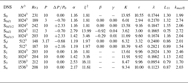
Table 1 summarises the physical and computational parameters of the DNS carried out in this work, together with several statistics corresponding to the final instant of each simulation, except for the final four (4) simulations, where the statistics correspond to an average taken over several fields/instants.

Table 1.

Physical and computational parameters of the DNS carried out in this work. The reported statistics correspond to the final instant of each simulation except for the last four simulations (S $_1$ , S $_2$ , S $_3$ and S $_4$ ), where the statistics represent an average over several fields/instants. S $_0$ is the initial (statistically stationary) reference DNS. Both S $_{0d1}$ and S $_{0d2}$ restart from this simulation, while simulations S $_{0d1i2}$ and S $_{0d1i3}$ both restart from S $_{0d1}$ (see text for details). The table contains also a single simulation with $80$ increasing/decreasing power cycles, where S $_{d}$ and S $_{u}$ represent the typical final status of each one of the cycles. Total number of colocation points ( $N^3$ ); Taylor-based Reynolds number ( $ \textit{Re}_{\lambda }$ ); external input power ( $P$ ); external input power variation ( $\Delta P/P_0$ ); constants of the forcing functions defined in (2.27), (2.25), (2.39) and (2.40) ( $\alpha$ , $\xi ^{2}$ , $\beta$ and $\gamma$ , respectively); turbulent kinetic energy ( $K$ ); viscous dissipation rate ( $\varepsilon$ ); Taylor micro-scale ( $\lambda$ ); longitudinal integral length scale ( $L_{11}$ ); resolution ( $k_{\textit{max}}\eta$ ). All the dimensional quantities, e.g. $K$ , are expressed in arbitrary units (as usual in DNS of HIT).

The first five DNS studies use a total of $N^{3}=1024^{3}$ collocation points and a kinematic viscosity of $\nu =0.0023$ (m $^2$ s⁻¹). The integral scale, indirectly imposed through the input forcing, is always kept sufficiently small (the box size is always much larger than the integral scale) to prevent confinement effects, while the resolution is always kept equal to, at least, $k_{\textit{max}} \eta \approx 2$ .

Each simulation case uses different forcing conditions that unbalance the previous flow condition imposing a new evolution trajectory. Here, S $_0$ is the initial (statistically stationary) reference DNS, obtained by allowing the flow to evolve in time, with the application of a (constant) external forcing function, $F(k)$ . Both S $_{0d1}$ and S $_{0d2}$ restart from this simulation by suddenly decreasing the magnitude of the external power input, but whereas in S $_{0d1}$ the shape of the forcing function is kept equal as in the simulation S $_0$ , ( $F_2(k)/P_2 = F_1(k)/P_1$ ), in an evolution of identically distributed forcing (IDF), in contrast, in S $_{0d2}$ , the forcing is also altered ( $F_2(k)/P_2 \ne F_1(k)/P_1$ ), i.e. variably distributed forcing (VDF). This is noticeable in the variation of the values of $\alpha$ and $\xi$ between these two simulations (see table 1). Finally, the simulations S $_{0d1i2}$ and S $_{0d1i3}$ both restart from the final field of S $_{0d1}$ , by suddenly increasing the external input power, but whereas in S $_{0d1i2}$ , the forcing shape is kept constant (IDF), in S $_{0d1i3}$ , it is altered (VDF).

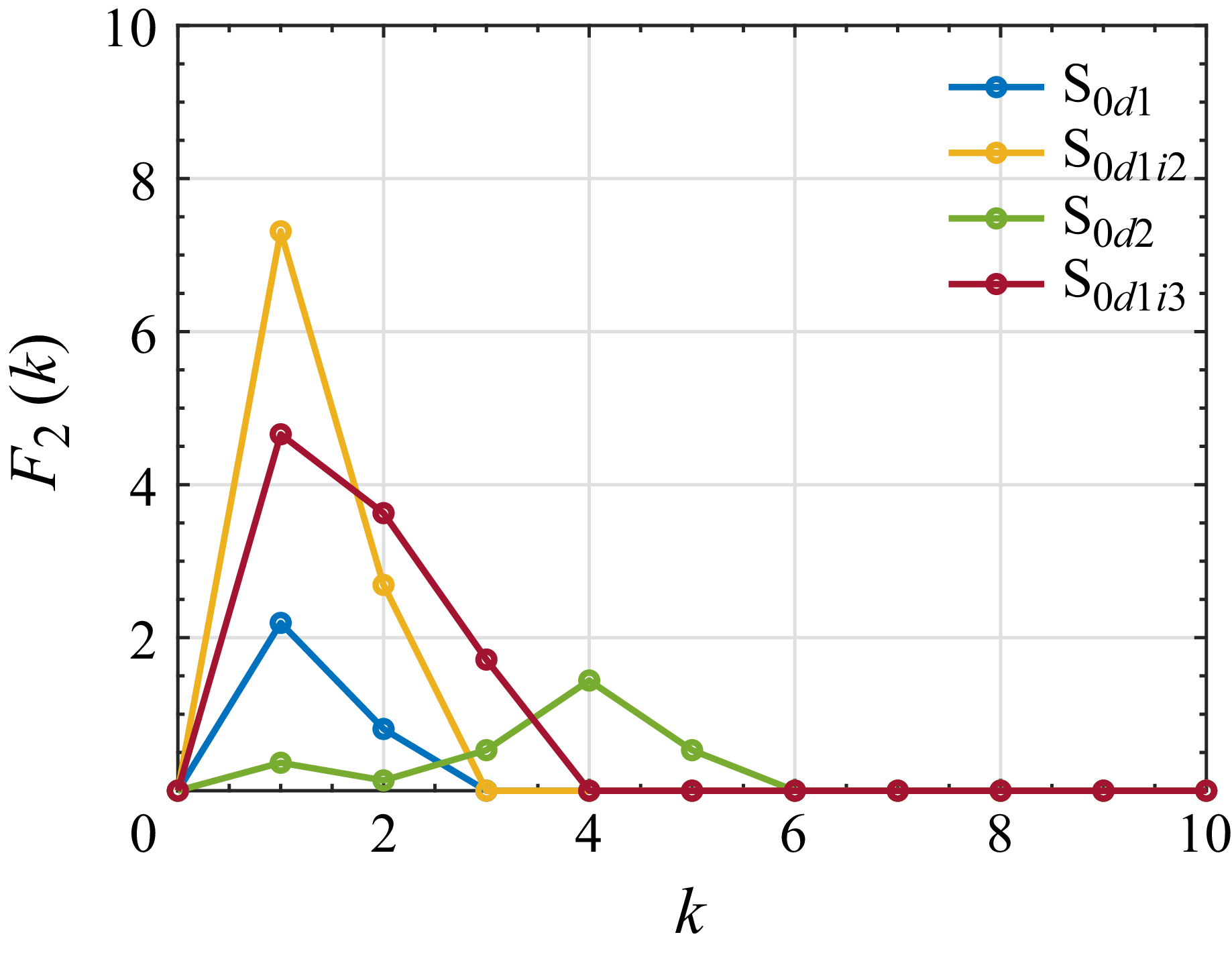
Figure 1 shows the forcing function applied at the start of each new simulation, $F_2(k)$ defined in the text right below (2.3), for all the DNS runs carried out in this work. The forcing function for the initial simulation (S $_{0}$ ) is not shown for clarity, since it is equal to the simulation S $_{0d1i2}$ . This forcing peaks at wavenumber $k_p = 1$ and has a power width of $\Delta k = 3$ . The forcing from the two decaying simulations that re-start from S $_{0}$ is quite different. Whereas in the case of S $_{0d1}$ (identically distributed forcing – IDF) the forcing function displays the same wavenumber peak and the same width of the forcing of S $_{0}$ , although with a smaller magnitude of the power input, the simulation S $_{0d2}$ represents VDF ( $F_2(k)/P_2 \ne F_1(k)/P_1$ ) with a wavenumber peak moved to $k_p=4$ , and with a power width increased to $\Delta k = 6$ . The forcing variation between S $_{0}$ and S $_{0d2}$ can be observed in figure 1, and also in the constants $\alpha$ and $\xi$ characterising the forcing listed in table 1, e.g. both $\alpha$ and $\xi$ are equal for S $_{0}$ and S $_{0d1}$ , but increase from S $_{0}$ to S $_{0d2}$ . Finally, for the power increasing simulations, both re-started from (the end of) S $_{0d1}$ , whereas S $_{0d1i2}$ keeps the same forcing of S $_{0d1}$ (see the values of $\alpha$ and $\xi$ from S $_{0d1}$ and S $_{0d1i2}$ ), S $_{0d1i3}$ increases the power width of the forcing.

Figure 1.

Forcing function $F_2(k)$ defined in (2.3) for DNS runs S $_{0d1}$ , S $_{0d1i2}$ , S $_{0d2}$ and S $_{0d1i3}$ . Note that simulation S $_{0}$ (not shown) uses the same forcing function of simulation S $_{0d1i2}$ .

For completeness, the computation of the constant $\xi ^2$ for simulation S $_{0d1i2}$ is now illustrated. Using the definition of this constant in (2.25) and with the help from figure 1, we can write

(3.14) \begin{align} \xi ^{2}=\frac {1}{P}\int _{0}^{\infty }F_{2}(k)k^{2}\,{\rm d}k \approx \big(7.31 \times 1^2 + 2.69 \times 2^2 \big)/10 \approx 1.81. \end{align}

The other constants are computed in a similar way for all the simulations.

An additional DNS is carried out with $N^3 = 512^3$ collocation points and a kinematic viscosity of $\nu =0.00391$ (m $^2$ s⁻¹) consisting of a total of 80 consecutive cycles of decreasing/increasing power input, and is carried out only to assess the shape of the kinetic energy spectra during the abrupt transient evolutions ( $S_u$ and $S_d$ ).

Finally, four additional DNS runs are carried out corresponding to statistical stationary cases, where the power input is kept constant, $P = \varepsilon$ , for the purpose of analysing the evolution of the non-dimensional dissipation with the forcing constant $\alpha$ . These simulations ( $S_1$ , $S_2$ , $S_3$ , and $S_4$ ) were designed to display approximately the same Reynolds number $ \textit{Re}_{\lambda } \approx 200$ , and the same power input $P = 10$ , with different values of the forcing constant $\alpha$ . In these simulations, the number of collocation points is equal to $N^3 = 1024^3$ or $N^3 = 1536^3$ and the kinematic viscosity is equal to $\nu =0.003, \,0.0023,\,0.00107$ and $0.00135$ (m $^2$ s⁻¹), for simulations S $_1$ , S $_2$ , S $_3$ and S $_4$ , respectively. These last four DNS runs are carried out for a long time, in the range of $23.42 \leqslant t_f / \left \langle \tau _{L} \right \rangle \leqslant 46.26$ , where $t_f$ is the total duration of the simulation and $\left \langle \tau _{L} \right \rangle$ is the mean integral time scale, defined as $\tau _{L} = L_{11} / u'$ . Naturally, for these DNS runs, the values listed in table 1 correspond to averages made up of several (statistically similar) fields.

4.1. DNS of isotropic turbulence under strong unsteady conditions

In this section, we use the DNS listed in table 1 to assess the theoretical results derived in § 2.

Figure 2 shows the evolution of several turbulent statistics from the time of their restart from the previous simulation, where the initial time is set to $t=0$ for each restarting simulation. The statistics are normalised by their initial value, e.g. the turbulent kinetic energy $K(t)$ is normalised by the value at the restart time $K_0 = K (t=0$ ). The qualitative behaviour of these statistics is very similar to that previously reported by Valente et al. (Reference Valente, Onishi and da Silva2014).

Figure 2.

Temporal evolution of turbulent statistics for the four strongly unsteady simulations listed in table 1: (a) S $_{0d1}$ ; (b) S $_{0d1i2}$ ; (c) S $_{0d2}$ and (d) S $_{0d1i3}$ . The statistics are normalised by their values at the initial time of the simulation: turbulent kinetic energy ( $K(t)/K_{0}$ ), viscous dissipation rate ( $\varepsilon (t)/\varepsilon _{0}$ ), longitudinal integral scale ( $L_{11}(t)/L_{110}$ ), Taylor-based Reynolds number ( $ \textit{Re}_{\lambda }(t)/Re_{\lambda 0}$ ) and non-dimensional dissipation rate ( $C_{\varepsilon }(t)/C_{\varepsilon 0}$ ). The time is normalised by the initial Kolmogorov time, $\tau _{\eta } (t=t_0) = \tau _{\eta } (0)$ .

Due to the sudden modification of the forcing at the start of the simulations, all statistics quickly evolve in time. As expected, and in agreement with (2.31), the turbulent kinetic energy suddenly decreases in simulations S $_{0d1}$ (figure 2 a) and S $_{0d2}$ (figure 2 c), because of the initial decrease of the power input $\Delta P\lt 0$ , and sharply increases in simulations S $_{0d1i2}$ (figure 2 b) and S $_{0d1i3}$ (figure 2 d), due to the initial power input rise in those cases ( $\Delta P\gt 0$ ). However, after this small transient by $t /\tau _{\eta } (0) \gtrsim 60$ ( $\Delta P\gt 0$ ) and $t /\tau _{\eta } (0) \gtrsim 120$ ( $\Delta P\lt 0$ ), the flow reaches a new situation of equilibrium since all the statistics have again attained a statistically stationary state.

As observed by Valente et al. (Reference Valente, Onishi and da Silva2014), the dissipation rate follows the same tendency as the kinetic energy, i.e. decreasing/increasing in the cases where the kinetic energy decreases/increases, respectively. This is also predicted by (2.34), for $\Delta P\lt 0$ / $\Delta P\gt 0$ , respectively. Moreover, the evolution of the dissipation rate follows that of the kinetic energy always with a small time lag, i.e. $\varepsilon$ is seen to decrease or increase appreciably only after $40 \tau _{\eta } (0)$ or $20 \tau _{\eta } (0)$ , respectively. A similar time lag has been previously observed and discussed by Horiuti & Tamaki (Reference Horiuti and Tamaki2013) and Valente et al. (Reference Valente, Onishi and da Silva2014) (and references therein), but can be seen to be a consequence of the equations derived in § 2. Recall that prior to the forcing modification, the flow is in a statistically stationary state so that we will have $\partial K^{-} / \partial t \approx \partial \varepsilon ^{-} / \partial t \approx 0$ , and whereas (2.31) shows that the time derivative of the turbulent kinetic energy $\partial K^{+} / \partial t$ is immediately affected by a sudden increase of the external power input forcing $\Delta P$ , the same is not true of the time derivative of the dissipation rate. Indeed, (2.34) shows that in the limit of infinite Reynolds number ( $\nu \rightarrow 0$ ), the time derivatives $\partial K^{+} / \partial t$ and $\partial \varepsilon ^{+} / \partial t$ are totally decoupled since in that case, $\partial \varepsilon ^{+} / \partial t \approx 0$ , regardless of the value of $\Delta P$ . Moreover, the fact that $\partial \varepsilon ^{+} / \partial t \approx 0$ is consistent with the reported time lag between $K(t)$ and $\varepsilon (t)$ discussed previously and in some previous works, e.g. Horiuti & Tamaki (Reference Horiuti and Tamaki2013) and Valente et al. (Reference Valente, Onishi and da Silva2014). Naturally, in an intermediate case, where the kinematic viscosity is very small (but not zero), (2.34) shows that a sudden modification in the forcing conditions will cause a negligible change in the dissipation rate derivative. The existence of a finite time lag between the evolutions of $K(t)$ and $\varepsilon (t)$ reflects the well-known large-scale/small-scale independence at high-Reynolds-number turbulence, and implies that any change made at large scales of motion will need time to be felt at the smallest scales of motion.

Finally, note that the dissipation rate can also change, i.e. $\partial \varepsilon ^{+} / \partial t \ne 0$ if the power input keeps the same magnitude, $\Delta P = 0$ , provided the power function changes its shape ( $\xi ^2 \ne \xi _0^2$ ). This is clearly illustrated by comparing the evolution of the dissipation rate in simulations S $_{0d1i2}$ and S $_{0d1i3}$ . In figure 2, it is clear that the time lag between $K(t)$ and $\varepsilon (t)$ is slightly bigger in simulation S $_{0d1i2}$ , where it lasts $\delta t /\tau _{\eta } (0) \approx 10$ (figure 2 b), than in S $_{0d1i3}$ , where we observe $\delta t /\tau _{\eta } (0) \approx 5$ (figure 2 d). The two simulations re-start from the same field (from simulation S $_{0d1}$ ), with the same (initial) Reynolds number of $ \textit{Re}_{\lambda } = 189$ , and use the same power variation, $\Delta P = P - P_0 = 10 - 3 = 7$ ( $\xi _0^2 = 1.81$ in both cases). However, in S $_{0d1i3}$ , the forcing is variably distributed (VDF) with $\xi ^2 = 3.46$ , while in S $_{0d1i2}$ , the forcing is identically distributed (IDF) with $\xi ^2 = \xi _0^2 = 1.81$ . By re-writing (2.34) as

(4.1) \begin{align} \frac {\partial \varepsilon ^{+}}{\partial t} = 2 \nu \big [ P \xi ^{2} - P_0 \xi _{0}^{2} \big ] + \frac {\partial \varepsilon ^{-}}{\partial t}, \end{align}

it is clear that $\partial \varepsilon ^{+} / \partial t$ must be higher in S $_{0d1i3}$ than in S $_{0d1i2}$ , due to its bigger value of $\xi ^2$ , and this is consistent with the smaller time lag observed for S $_{0d1i3}$ compared with S $_{0d1i2}$ . In other words, as remarked by an anonymous referee, since in simulation S $_{0d1i3}$ the effective Taylor-scale of the forcing $\xi$ is smaller than in simulation S $_{0d1i2}$ , the forcing is directly injected closer to the smallest dissipative scales and, naturally, the observed time lag for this simulation (S $_{0d1i3}$ ) must be also smaller.

As expected, the longitudinal integral scale $L_{11}(t)$ adjusts quickly to the initial disturbance, and seems to be settling at $t /\tau _{\eta } (0) \approx 40$ (for S $_{0d1i2}$ and S $_{0d1i3}$ ) or $t /\tau _{\eta } (0) \approx 80$ (for S $_{0d1}$ and S $_{0d2}$ ), like the turbulent kinetic energy, and it shares also with $K(t)$ the absence of a delay in the adjustment to the changing forcing conditions. This is to be expected from the analysis of (2.36), where one can notice also that an increase/decrease of the power input $\Delta P$ leads to an instantaneous positive/negative evolution of $\partial L_{11}^{+}/\partial t$ , respectively, even for infinite Reynolds numbers. Equation (2.36) further shows that the temporal evolution of $L_{11}(t)$ is governed by its initial value $L_{110}$ , and by the ‘distribution’ of the forcing function through the constants $\alpha$ and $\alpha _0$ in the second term on the right-hand side of (2.36). In particular, an IDF, i.e. $\alpha = \alpha _0$ , cancels the second term on the right-hand side of (2.36) leading to a relatively ‘small’ variation of $L_{11}(t)$ (e.g. S $_{0d1}$ – figure 2 a). Conversely, when the power input decreases/increases ( $\Delta P\lt 0$ / $\Delta P\gt 0$ ), and simultaneously, the forcing wavenumber increases/decreases (by increasing/decreasing $\alpha$ in relation to $\alpha _0$ ), this second term on the right-hand side of (2.36) becomes more important (and negative/positive) leading to a very sharp evolution of $L_{11}(t)$ (e.g. S $_{0d1i2}$ and S $_{0d2}$ – figure 2 b,c). Finally, when these two effects are opposite, the variation of $L_{11}(t)$ is slower (S $_{0d1i3}$ – figure 2 d).

The analytical result derived in (2.18) is compared with the results from the unsteady DNS in figure 3, where to allow for this comparison, we write (2.18) as

(4.2) \begin{align} C_{\varepsilon }\left (Re_{\lambda }\right )=g_{i}\left [Re_{\lambda }(t)\right ]^{p_{i}} \,, \end{align}

with the subscript ‘ $i$ ’ being used to label each case, e.g. $g_{0d1}$ is the value of $g_i$ for case S $_{0d1}$ and $p_{0d1}$ is the power law obtained for simulation $S_{0d1}$ . Figure 3 shows the non-dimensional dissipation rate $C_{\varepsilon }$ as function of Taylor-based Reynolds number $ \textit{Re}_{\lambda }$ , for each simulation. In all but one of the simulations (S $_{0d2}$ ), the $C_{\varepsilon } = C_{\varepsilon } (Re_{\lambda })$ exhibits a characteristic $\vee$ or $\wedge$ shape, already observed by Valente et al. (Reference Valente, Onishi and da Silva2014). Here, S $_{0d1}$ and S $_{0d2}$ restart from the same point (denoted in the figures by a ‘ $+$ ’) and evolve by the application of an equal level of the power input $P = 3$ , which decreases from $P_0=10$ in the original (previous) simulation (S $_0$ ); however, in S $_{0d2}$ , the power is applied in a much larger wavenumber, which explains why a smaller final Reynolds number is attained. Simulations S $_{0d1i2}$ and S $_{0d1i3}$ also restart from the same point – the end of simulation S $_{0d1}$ (denoted by an ‘ $\times$ ’ in the figures), and use the same input power $P=10$ ; however, in S $_{0d1i2}$ , this is applied at smaller wavenumbers, which explains why a higher maximum (instantaneous) Reynolds number is attained in that simulation.

Figure 3.

Non-dimensional dissipation rate $C_{\varepsilon }$ as a function of Taylor-based Reynolds number $ \textit{Re}_{\lambda }$ for all the DNS runs S $_{0d1}$ , S $_{0d1i2}$ , S $_{0d2}$ and S $_{0d1i3}$ , compared with power laws for each case (straight lines). The curves of $C_{\varepsilon }$ obtained from the simulations are the same in both figures, but whereas in panel (a) the power laws are computed with (2.15) and (2.17) with $H=H(0)$ (exact), in panel (b), the power laws are computed with (2.38). The constants, e.g. $g_{0d1i2}$ , are computed with (2.18). The ‘ $+$ ’ denotes the starting point for simulations S $_{0d1}$ and S $_{0d2}$ , while the ‘ $\times$ ’ indicates the start of simulations S $_{0d1i2}$ and S $_{0d1i3}$ .

The initial evolution of $C_{\varepsilon }$ is compared with power laws represented by straight lines, where the values of the power laws, e.g. $p_{0d1}$ , were computed without any simplification using (2.15) in figure 3(a) and by using strong unsteadiness condition leading to (2.38) in figure 3(b).

It is clear that the DNS results are well approximated by the computed power laws given by these equations and, as expected, the agreement is slightly better when using the exact relation (figure 3 a) than when using the strong unsteadiness condition (figure 3 b); however, the agreement is also remarkably good in this case, which testifies to the robustness of this approximation expressed through (2.38). The fact that the observed exponents are different for S $_{0d1}$ and S $_{0d2}$ can only be explained by the difference in the shape of the applied forcing, since everything else is kept the same. An identical conclusion is reached when comparing S $_{0d1i2}$ and S $_{0d1i3}$ .

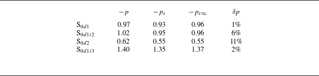
Table 2 shows the values of the power law $p$ obtained straight from the DNS data, and by using the approximations in (2.38) representing strong unsteadiness conditions and (2.42) representing strong unsteadiness conditions in the limit of infinite Reynolds number. Higher values of $-p$ are obtained whenever the input power increases ( $\Delta P \gt 0$ ) – S $_{0d1i2}$ and S $_{0d1i3}$ – and it is noteworthy that the value of $p$ is in the range of $1.02 \leqslant -p \leqslant 1.40$ , which compares well with the value of $- p = 1.1{-}1.2$ observed in several experimental and numerical works involving non-equilibrium turbulence (Vassilicos Reference Vassilicos2015). Comparatively smaller values of $-p$ correspond to situations of input power decay ( $\Delta P \lt 0$ ) – S $_{0d1}$ and S $_{0d2}$ . In all cases, the approximations given here for $p$ are quite close to its exact values, thus attesting the quality of these approximations.

Table 2.

Results for the power law $p$ obtained in simulations S $_{0d1}$ , S $_{0d1i2}$ , S $_{0d2}$ and S $_{0d1i3}$ : $p$ is the exact value of the power law obtained directly from the simulations through (2.15) and (2.17) with $H=H(0)$ (exact), $p_{s \infty }$ is the value of $p$ computed using the infinite Reynolds number approximation (together with the strong unsteadiness condition) defined in (2.42) and $p_{s}$ is the value of $p$ computed with strong unsteadiness condition defined in (2.38). $\delta p$ is the error between $p$ and $p_{s \infty }$ .

Figure 4 shows the temporal evolution of the term $ [H (t )-2 ]$ , where $H(t)$ is computed using the DNS data, straight from its definition given by (2.15). Recall that from (2.17), whenever $H(t)$ is constant, the power law constant $p$ is equal to $p = H - 2$ , or considering very small times, $p = p^{+} = \lim _{t\rightarrow 0^{+}} [ H (t ) - 2 ]$ (see (2.37)). The curves of $H(t) - 2$ are compared with the value of $p$ given by (2.38). The results show that increasing/decreasing the external power input leads to a different behaviour of $H (t )-2$ . When the power input increases ( $\Delta P\gt 0$ ) as in simulations S $_{0d1i2}$ and S $_{0d1i3}$ , $H (t )-2$ is constant for a small time interval of $t /\tau _{\eta } (0) \approx 10{-}15$ (figures 4 b and d). Conversely, whenever the external power input decreases ( $\Delta P\lt 0$ ), as in simulations S $_{0d1}$ and S $_{0d2}$ , $H (t )-2$ fluctuates around a constant value for $t /\tau _{\eta } (0) \approx 30-40$ . Recall that a constant value of $H (t )-2$ , for a short initial time, is to be expected according to (2.16) if $C_{\varepsilon }$ is to follow a power law of the turbulent Reynolds number defined by (2.17).

Figure 4.

Temporal evolution of $[H(t)-2]$ for all the strongly unsteady DNS carried out in the present work (S $_{0d1}$ , S $_{0d1i2}$ , S $_{0d2}$ and S $_{0d1i3}$ ), compared with the values of the power law constant $p$ computed from (2.38), represented by straight lines: (a) S $_{0d1}$ ; (b) S $_{0d1i2}$ ; (c) S $_{0d2}$ and (d) S $_{0d1i3}$ .

To understand the origin of the small deviation from the power law (2.16) observed for cases S $_{0d1}$ and S $_{0d2}$ , we analyse the short-time behaviour of the evolution of $C_{\varepsilon } (t)$ by expanding the exact expression of $H(t)$ to first order in time,

(4.3) \begin{align} H(t)\approx H_{0}+H_{0}'\Delta t \,, \end{align}

where $H_{0}=\lim _{t\rightarrow 0^{+}} H (t )$ and $H_{0}'=\lim _{t\rightarrow 0^{+}} {{\rm d} H (t )}/{{\rm d}t}$ . Since we aim to express $H (t )$ and $C_{\varepsilon }(t)$ in terms of the Reynolds number $ \textit{Re}_{\lambda }$ , we also consider the expansion,

(4.4) \begin{align} Re_{\lambda } (t) \approx Re_{\lambda 0} + Re_{\lambda 0}'\Delta t, \end{align}

where similarly, $ \textit{Re}_{\lambda 0} = \lim _{t\rightarrow 0^{+}} Re_{\lambda } (t )$ and $ \textit{Re}_{\lambda 0}'=\lim _{t\rightarrow 0^{+}} {{\rm d} Re_{\lambda } (t )}/{{\rm d}t}$ . Using (4.3) and (4.4) to eliminate $\Delta t$ , we obtain

(4.5) \begin{align} H(t)\approx H_{0}+\frac {H_{0}'}{R_{0}'}\left (Re_{\lambda } - Re_{\lambda 0} \right ). \end{align}

Inserting this expression in (2.14) and solving the resulting differential equation, we arrive at

(4.6) \begin{align} \frac {C_{\varepsilon }(t)}{C_{\varepsilon 0}} = \left [ \frac {Re_{\lambda }(t)}{Re_{\lambda 0}} \right ]^{H_{0} - 2 - \frac {H_{0}'}{Re_{\lambda 0}'} Re_{\lambda 0} } \exp \left [ \frac {H_{0}'}{Re_{\lambda 0}'}\left (Re_{\lambda } (t) - Re_{\lambda 0}\right ) \right ] \!. \end{align}

It should be emphasised that this result is only valid in the regime $ ( Re_{\lambda } - Re_{\lambda 0} ) / Re_{\lambda 0} \ll 1$ , since for larger deviations, higher-order terms in the expansion of $H(t)$ must be considered, nevertheless, for $ \textit{Re}_{\lambda } \neq Re_{\lambda 0}$ but $ \textit{Re}_{\lambda } \approx Re_{\lambda 0}$ , the exponential term is approximately $1.0$ and the remaining factor represents a power law with exponent $\tilde {p} = H_{0} - 2 - ({H_{0}'}/{Re_{\lambda 0}'})Re_{\lambda 0}$ , where $\tilde {p}$ is the power law for this particular (asymptotic) case. Recalling that $p = H_0 - 2$ , we identify the deviation as arising from the term $({H_{0}'}/{Re_{\lambda 0}'}) Re_{\lambda 0}$ . In the specific case where $H_0' \gt 0$ and $ \textit{Re}_{\lambda 0}' \lt 0$ , it follows that $({H_{0}'}/{Re_{\lambda 0}'}) Re_{\lambda 0} \lt 0$ , implying $\tilde {p} \gt p$ , which is indeed observed.

The differences between the two cases of increasing/decreasing power input might be explained by the time scales associated with the dynamical adjustment underway. Of course, in both cases, when the power input is suddenly modified, the modification occurs at the large scales of motion, which are associated with a much larger time scale than that of the smallest scales of motion which typically adjust very fast to any imbalance. However, when the power input is increased, since the modification is imposed by the forcing function, which is applied to those scales, this is immediately imposed on the large scales of motion, i.e. there is no delay or time lag between the actuation of the forcing and the modification of the large scales of motion, leading to a situation where the large scales have been suddenly changed to which only the small scales need to adjust. However, when the power forcing is decreased, the situation is slightly different because the large scales of motion will not adjust instantaneously to the forcing function, and this delay, between the instantaneous modification of the forcing function and the modification of the large scales of motion, will need some adjustment time. We will return to this discussion later.

Finally, after this initial transient, where an approximately constant value of $p$ is observed, $C_{\varepsilon }$ evolves in a complex way, without a clear power law, until later times, e.g. for $t /\tau _{\eta } (0) \gtrsim 40$ in simulation S $_{0d1i2}$ , where a new region in which $p$ is roughly constant is again visible, with $p$ close to $-2$ (or $H (t )\approx 0$ ). Now, by combining (2.13) and (2.14), we can write $H (t )$ as (see Appendix A)

(4.7) \begin{align} H(t) = \frac {Re_{\lambda }(t)}{Re_{L}(t)} \frac {\partial Re_{L}(t)}{\partial Re_{\lambda }(t)} \,, \end{align}

which shows that a region with $H (t )\approx 0$ implies that $\partial Re_{L}/\partial Re_{\lambda } \approx 0$ . Since $ \textit{Re}_{L} (t )$ is exclusively defined by the largest scales of motion ( $u'(t)$ and $L_{11}(t)$ ), whereas $ \textit{Re}_{\lambda } (t )$ involves also the effects of the smallest scales of motion through the definition of $\lambda (t)$ , a constant power law region with $H (t )\approx 0$ arises in situations where the large scales of motion are already ‘settled’, while the smallest scales of the flow are still adjusting. Notice that this is observed in situations where we have a particularly strong unsteadiness and where the $ \textit{Re}_{\lambda }$ is sufficiently high, such as in simulations S $_{0d1i2}$ (figure 4 b) and S $_{0d1i3}$ (figure 4 d), but not in the other cases.

Going back again to the analysis of figure 4, we now focus on the behaviour of $H(t)-2$ for small times. As discussed previously, in some simulations, e.g. S $_{0d1i2}$ , $H(t)-2$ is approximately constant for small times, as expected from the theoretical relations derived in § 2.3, while in other simulations, e.g. S $_{0d1}$ , a similar plateau (for small times) is not observed. It is argued previously that the differences have to do with the fact that in power increasing situations, the large scales of motion react much faster than in power decreasing cases.

To see this in detail, we now turn to simulation S $_{d}$ /S $_{u}$ listed in table 1 which represents a single simulation with $80$ increasing/decreasing power cycles, where S $_{d}$ and S $_{u}$ are the final state of each one of the cycles. Figure 5(a) shows the temporal evolution of the normalised turbulent kinetic energy for 10 of the 80 cycles of this simulation, where as in figure 2, the normalisation is done with the initial values of these quantities. The figure shows the variability of the power increasing/decreasing cycles; however, even here, a closer look allows one to observe differences in the two situations. This is seen in the behaviour of the dissipation rate that exhibits stronger and more ‘active’ spikes for increasing than in decreasing power events. A closer look into this can be perceived in figure 5(b) showing ensemble-averaged evolutions of these quantities for small times, where all the 80 cycles are used in the averaging, e.g. $\left \langle K / K_0 \right \rangle _{80}$ is the normalised temporal evolution of the turbulent kinetic energy for small times, averaged over the whole temporal series. It is clear that after an increase of the input power, both the turbulent kinetic energy and the viscous dissipation rate deviate from the initial normalised value of $1$ much more then when the input power is decreased. Moreover, both quantities exhibit peaks after the power increase that are absent in power decreasing cycles. This shows that the flow behaves very differently in increasing and decreasing power inputs.

Figure 5.

(a) Temporal evolution of the normalised turbulent kinetic energy and viscous dissipation rate for 10 cycles of the simulation S $_{u}$ /S $_{d}$ (which includes a total of 80 cycles); (b) ensemble average (using 80 cycles) of the temporal evolution of the kinetic energy and viscous dissipation rate for small times. The Taylor-based Reynolds number is also shown (the solid/dashed lines correspond to events of power increase/decrease, respectively).

Figure 6 shows the kinetic energy spectra $E(k,t)$ for simulations S $_{u}$ and S $_{d}$ , where each line corresponds to a single time instant and each instant is separated by the same time interval (equal in both simulations). As expected, the kinetic energy spectrum is increasing with time in simulation S $_{u}$ and is decreasing as time progresses in simulation S $_{d}$ . Also, the individual lines for $E(k,t)$ approach for the last instants in both simulations, indicating that $E(k,t)$ is tending to an approximately constant shape, representing the end of the transient region. However, it is clear that for the first few instants, the variation of $E(k,t)$ for S $_{u}$ is much faster than for S $_{d}$ . This is particularly clear when looking at the insets of both figures and shows unambiguously that the kinetic energy spectrum evolves much faster in a situation of increasing external power input than in a situation of decreasing power input.

Figure 6.

Temporal evolution of the kinetic energy spectra for simulations S $_{u}$ and S $_{d}$ right after variation of the external power input: (a) S $_{u}$ ; (b) S $_{d}$ . Each line corresponds to a single instant and the lines for both simulations are spaced with the same (constant) time interval, corresponding to a few hundred iterations. The arrows represent the direction of time.

4.2. DNS of isotropic turbulence in statistically steady conditions

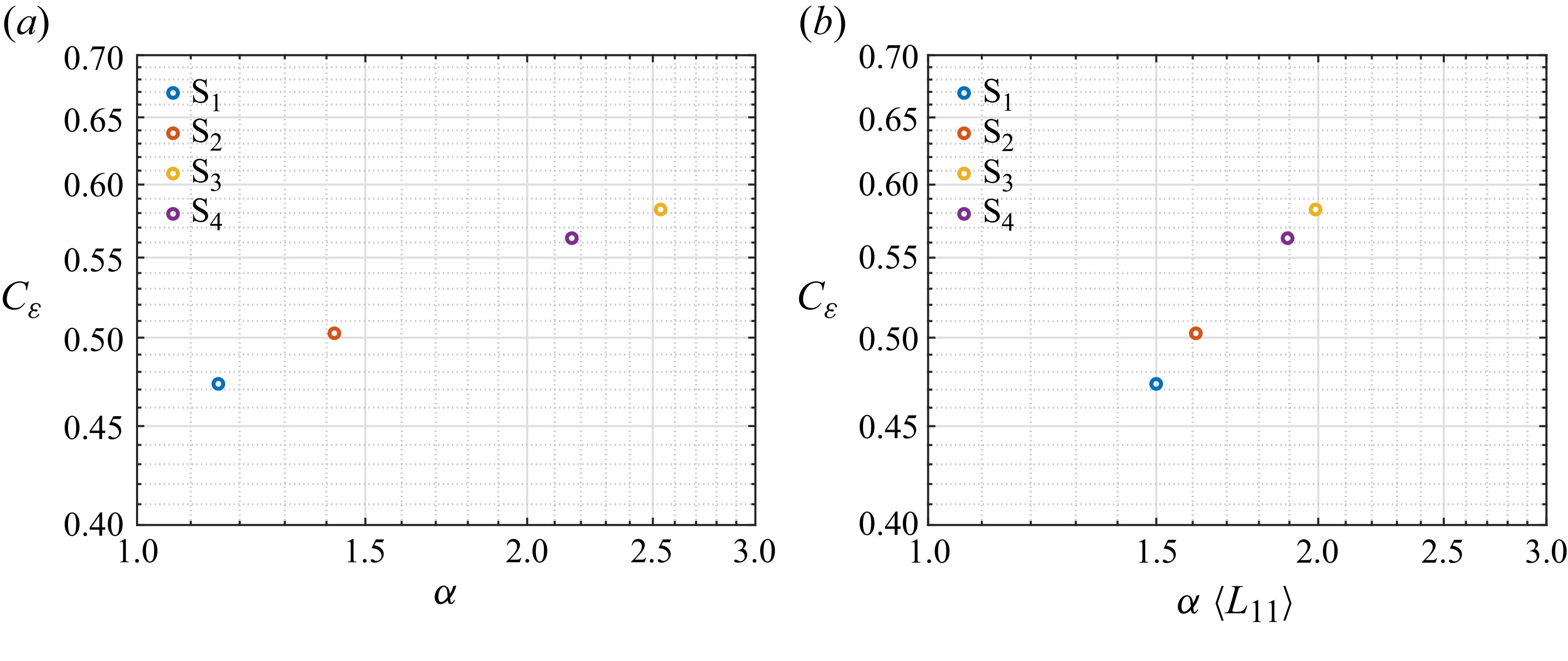
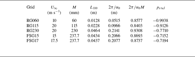
This section deals with forced HIT in statistically steady forcing conditions. The goal is to assess the assumption made by Sreenivasan (Reference Sreenivasan1998) that the asymptotic value of the normalised dissipation rate, observed in high-Reynolds-number turbulent flows, is imposed by the large scales of motion. In other words, the different values of $C_{\varepsilon }$ observed in different (statistically steady) flows reflect different characteristics of the large-scale forcing. In the present configuration (forced HIT), this consists in observing the dependency of the non-dimensional dissipation on the characteristics of the external input forcing and, in particular, of the value of the non-dimensional forcing constant, $\alpha$ .

Indeed, in the previous section, we saw that the value of the power $p$ in the experimental law $C_{\varepsilon } \sim Re_{\lambda }^p$ is well predicted by the new theoretical result defined in (2.43), i.e. the value of the exponent $p$ depends only on the values of the forcing constant $\alpha$ and on the value of initial longitudinal integral scale $L_{110}$ : $p \approx 3\pi / 4\alpha L_{110} - 5/2$ , which clearly shows that the power $p$ is strictly imposed by the large scales of motion. This new theoretical result (valid for strongly unsteady forcing and high Reynolds numbers) then strongly suggests that the large scales of motion also impose the value of the non-dimensional dissipation $C_{\varepsilon }$ , i.e. for the same value of the Reynolds number, $C_{\varepsilon }$ is imposed by the large-scale forcing (and initial integral scale of motion). Does something similar occur for statistically stationary turbulence when we consider the mean value of $C_{\varepsilon }$ ?

To assess this question, four statistically stationary DNS runs were carried out (S $_1$ , S $_2$ , S $_3$ and S $_4$ ), with approximately the same Reynolds number ( $ \textit{Re}_{\lambda } \approx 200$ ), but with different values of the forcing constant $\alpha$ (see table 1), which is achieved by varying the kinematic viscosity. Note that $ \textit{Re}_{\lambda } \approx 200$ is sufficiently large such that the statistically steady $C_{\varepsilon }$ is Reynolds number independent (e.g. Sreenivasan Reference Sreenivasan1998; Ishihara et al. Reference Ishihara, Gotoh and Kaneda2009), i.e. the present DNS are valid for assessing the dependence of $C_{\varepsilon }$ on the large scales of motion at high Reynolds numbers, whereas the works cited are concerned with the asymptotic behaviour of turbulent flows in the limit of infinite Reynolds numbers.

Figure 7(a) shows the temporal evolution of several turbulence quantities for DNS S $_1$ . All the quantities were computed as described in § 3.1, e.g. $ \textit{Re}_{\lambda } (t)$ is computed with (3.11). As expected, the turbulent kinetic energy, dissipation rate and integral scale all fluctuate around their mean values, and consequently, the normalised dissipation also fluctuates during the simulation. The other simulations show similar qualitative results (not shown). Figure 7(b) shows the instantaneous value of $C_{\varepsilon }$ as a function of the instantaneous Reynolds number for the four statistically stationary simulations. As expected, the instantaneous value of the non-dimensional dissipation oscillates with the instantaneous value of the Reynolds number, however, four different regions corresponding to the four different Reynolds numbers are clearly visible. Specifically, higher values of $C_{\varepsilon }$ tend to exist for higher values of $\alpha$ , which is clear evidence that $C_{\varepsilon }$ depends on the forcing scale. So, both $C_{\varepsilon }$ and its scaling exponent $p$ in non-equilibrium conditions, which is given by (2.43) depend on the large scales and the forcing characteristics.

Figure 7.

(a) Temporal evolution of turbulent statistics for simulation S $_1$ normalised by their mean values: turbulent kinetic energy $K(t)/\langle K \rangle$ , viscous dissipation rate $\varepsilon (t)/\langle \varepsilon \rangle$ , longitudinal integral scale $L_{11}(t)/\langle L_{11} \rangle$ , Taylor-based Reynolds number $ \textit{Re}_{\lambda }(t)/\langle Re_{\lambda } \rangle$ and non-dimensional dissipation $C_{\varepsilon }(t)/\langle C_{\varepsilon } \rangle$ . (b) Temporal evolution of the non-dimensional dissipation $C_{\varepsilon } (t)$ as a function of the power constant $\alpha$ for all the statistically stationary simulations S $_1$ ( $ \textit{Re}_{\lambda } = 203$ ), S $_2$ ( $ \textit{Re}_{\lambda } = 204$ ), S $_3$ ( $ \textit{Re}_{\lambda } = 212$ ) and S $_4$ ( $ \textit{Re}_{\lambda } = 208$ ) – see table 1. The time is normalised by the eddy-turnover time, $\tau _L = L_{11}/u'$ .

An even more compelling demonstration of the influence of the forcing on the determination of $C_{\varepsilon }$ can be gained by looking into figures 8(a) and 8(b) showing the variation of the mean values of the non-dimensional dissipation with the forcing constant $\alpha$ and with the product of this constant with the initial longitudinal integral scale $L_{110}$ , for similar values of the Reynolds number. The figures suggest the existence of linear relation between both $C_{\varepsilon }$ and $\alpha$ and between $C_{\varepsilon }$ and $\alpha L_{110}$ , thus again demonstrating that both $\alpha$ and $L_{110}$ impose the value of $C_{\varepsilon }$ also in statistically steady conditions.

Figure 8.

Variation of the non-dimensional dissipation ( $C_{\varepsilon }$ ) with the forcing constant ( $\alpha$ ) and longitudinal integral scale ( $L_{11}$ ), for the four statistically stationary simulations, with approximately the same Reynolds number, S $_1$ ( $ \textit{Re}_{\lambda } = 203$ ), S $_2$ ( $ \textit{Re}_{\lambda } = 204$ ), S $_3$ ( $ \textit{Re}_{\lambda } = 212$ ) and S $_4$ ( $ \textit{Re}_{\lambda } = 208$ ) – see table 1: (a) $C_{\varepsilon }$ versus $\alpha$ ; (b) $C_{\varepsilon }$ versus $\alpha \langle L_{11} \rangle$ .

The present results confirm a forcing dependence, as previously suggested by Sreenivasan (Reference Sreenivasan1998), and further show how $C_{\varepsilon }$ can be manipulated by adjusting the shape of the forcing spectrum, i.e. $\alpha$ . Furthermore, the results in figure 7 (b) reveal that increasing $\alpha$ reduces the fluctuations of $C_{\varepsilon }$ around its statistically steady value. This may be explained by the fact that $L_{11}$ is reduced when increasing $\alpha$ and, hence, a greater number of large-scale structures is contained within the computational domain, which improves convergence at any given time instant. The sensitivity of $C_{\varepsilon }$ on the forcing details may also explain the scatter in the reported values for $C_{\varepsilon }$ , see for example figure 2 of Ishihara et al. (Reference Ishihara, Gotoh and Kaneda2009). The values of the non-dimensional dissipation at the asymptotic (high-Reynolds-number) regime (starting at $ \textit{Re}_{\lambda } \approx 200$ ) are close to $0.5$ ; however, they are clearly not equal for all the simulations, which probably reflects the effect of the different forcing conditions used by the different numerical codes. The same comment can be made regarding table 1 of Sreenivasan (Reference Sreenivasan1998), where the values of $C_{\varepsilon }$ vary quite substantially, not only between forced and decaying homogeneous turbulence, but also within these two classes of flows, and the differences between $C_{\varepsilon }$ in the decaying cases probably reflect differences in the initial large scales characteristics.

An attempt at explaining these results can be described as follows: in stationary statistically DNS, the dissipation rate, $\varepsilon$ , is kept constant (on average) due a constant power input. Since the non-dimensional dissipation can be written as $C_{\varepsilon } = \varepsilon L_{11}/(2/3K)^{3/2}$ and we observe $L_{11} \propto K$ (based on data for S $_1$ , S $_2$ , in table 1), this shows that $C_{\varepsilon } \propto L_{11}^{-1/2}$ . We can interpret $\alpha$ as the effective forcing wavenumber. Hence, a higher $\alpha$ implies a higher forcing wavenumber and consequently a smaller integral scale $L_{11}$ . The result that $C_{\varepsilon }$ increases with increasing $\alpha$ is consistent with our observations. Finally, the fact that $K \propto L_{11}$ is consistent with (2.31) and (2.36), even if these cannot be rigorously used in the context of equilibrium turbulence. Indeed, (2.31) shows that a variation in power input $\Delta P$ is immediately felt in $K$ , and (2.36) similarly implies the same thing for $L_{11}$ .

Even if, at present, a clear explanation cannot be given for the results of statistically stationary turbulence, these results are worth reporting since they show that even in this simpler case (of statistically stationary turbulence), the large scales impose the value of $C_{\varepsilon }$ . Thus, the huge scatter in $C_{\varepsilon }$ reported by Sreenivasan (Reference Sreenivasan1998) and Ishihara et al. (Reference Ishihara, Gotoh and Kaneda2009) highlights the importance of the large scales of motion and, more specifically, of the different forcing schemes that impose the large-scale characteristics.

4.3. Experimental data from the literature on decaying grid turbulence

We close this section by demonstrating the generality of the results derived in this paper, by comparing the new theoretical relations derived in § 2.3 with experimental results from the literature.

The rationale for doing this comparison is the following. In grid-generated turbulence, a clean stream of air is driven across a grid of bars (or a fractal grid), where turbulence is ‘locally’ generated, followed by a small region where the turbulence adjusts to the grid. This is then followed by a decaying turbulence region, where turbulence slowly decays with the downstream distance from the grid ( $x$ ). The boundary between the initial adjustment region and the decaying region is marked by the downstream coordinate $x^{\ast }$ , where the turbulent kinetic energy attains its peak. We can draw a parallel between the localised turbulent kinetic energy created by the grid and the abrupt turbulent kinetic energy injected by the (unbalanced) forcing in a DNS of HIT. In both cases, turbulence needs to adjust to a strong initial ‘perturbation’ and the assumptions behind the theoretical results derived in § 2.3 can be used.

We focus on the results described by Valente & Vassilicos (Reference Valente and Vassilicos2012), who measured isotropic turbulence decay downstream of several regular and square fractal grids. Their measurements started very close to the grids and covered (for each grid) two different decaying regions: an initial (first) decay region where the non-dimensional dissipation varies with the Reynolds number following a power law, as in (2.16), with $p \ne 1$ , where turbulence is in a non-equilibrium regime, followed by a second decaying region where the non-dimensional dissipation is independent of the Reynolds number ( $p = 0$ ), thus describing classical equilibrium turbulence.

Figures 9(a) and 9(b) show the evolution of the non-dimensional dissipation $C_{\varepsilon }$ , and of the ratio between the longitudinal integral scale and the Taylor micro-scale, $L_{11}/\lambda$ , as a function of the Taylor-based Reynolds number $ \textit{Re}_{\lambda }$ , respectively. The two regimes described here are well observed for the grid RG060. Initially, for higher values of $ \textit{Re}_{\lambda }$ ( $120 \lesssim Re_{\lambda } \lesssim 180$ ), the non-dimensional dissipation varies with the Reynolds number, and further downstream from the grid corresponding to lower values of $ \textit{Re}_{\lambda }$ ( $90 \lesssim Re_{\lambda } \lesssim 120$ ), the non-dimensional dissipation is approximately constant (figure 9 a). The evolutions of the ratio $L_{11}/\lambda$ shown in figure 9(b) are consistent with these results, showing two different power laws with the Reynolds number, corresponding to the first and second decay region, in agreement with (2.19) and (2.20), respectively.

Figure 9.

Experimental data from Valente & Vassilicos (Reference Valente and Vassilicos2012) showing (a) non-dimensional dissipation $C_{\varepsilon }$ , and (b) ratio between the longitudinal integral scale and the Taylor micro-scale $L_{11}/\lambda$ , as a function of the Taylor-based Reynolds number $ \textit{Re}_{\lambda }$ . RG and FSG stand for regular and square fractal grids, listed byValente & Vassilicos (Reference Valente and Vassilicos2012). The lines correspond to the power $p$ obtained from the data by fitting (2.20).

The value of the power $p$ in (2.20) was computed from the experimental data in figure 9(a) by using the data at point $x^{\ast }$ . Specifically, with the values of $\lambda / L_{11}$ obtained by Valente & Vassilicos (Reference Valente and Vassilicos2012), one uses a least-squares method to obtain the straight lines that better approximate the data and, from these, one gets the power $p$ by using $\lambda / L_{11} \sim Re_{\lambda }^{-(p+1)}$ – (2.20). Figure 9(b) shows the obtained straight lines for each case together with the data of Valente & Vassilicos (Reference Valente and Vassilicos2012). The Taylor micro-scale was computed using the definition of the Taylor-based Reynolds number and the root-mean-square of the streamwise velocity fluctuations, $u^{\prime} = \sqrt {\overline {u^{\prime 2}}}$ .

It is clear that different values of $p$ are obtained from the data in the non-equilibrium turbulence regime, with $p$ varying in the range of $-0.9938 \leqslant p \leqslant -0.7194$ (see the following when discussing table 3), i.e. the particular case $p \approx -1$ is only observed for one case (RG060). Moreover, the values of $p$ fitted to the data using figure 9(b) are also shown in figure 9(a), by using the law $C_{\varepsilon } \sim Re_{\lambda }^p$ , which agrees well with the experimental data, as expected.

Finally, we show that the non-dimensional forcing constant $\alpha$ defined in (2.27) and appearing in the theoretical result of (2.43) can be directly related to the grid characteristics, and represents the effective wavenumber imposed by the grid. This demonstrates the general validity of (2.43).

We start by showing that in the experimental data used here, there is a direct link between the initial value of the longitudinal integral scale $L_{110}$ and the characteristic grid size $M$ . In other words, the value of $M$ imposes the initial value of $L_{11}$ . This is observed in figure 10(a) showing the value of $L_{110}$ as function of $M$ for all the grids used by Valente & Vassilicos (Reference Valente and Vassilicos2012), where, as before, the value of $L_{110}$ corresponds to $L_{11}$ taken from the point of maximum turbulent kinetic energy i.e. at the start of the turbulence decaying region, $x^{\ast }$ . It is clear from this figure that $L_{110} \sim M$ , regardless of the type of grid used. This result is not surprising considering that the largest flow structures created by the grid originate in the initial instabilities in the wakes created by the largest ‘objects’ forming the grid.

Figure 10.

(a) Initial longitudinal integral scale $L_{110}$ (m) and (b) effective forcing wave number $2\pi /\alpha _0$ , as function of the characteristic length scale of the grid $M$ (m), for the grids listed by Valente & Vassilicos (Reference Valente and Vassilicos2012); RG and FSG stand for regular and square fractal grids, listed by Valente & Vassilicos (Reference Valente and Vassilicos2012). The dashed lines represent arbitrary linear relations used to see the linear relation between the quantities shown in the figures.

Figure 10(b) shows $2 \pi /\alpha _0$ , where $\alpha _0$ is the forcing constant defined by (2.27), as function of the characteristic grid size $M$ for all the grids used by Valente & Vassilicos (Reference Valente and Vassilicos2012). In this figure, the constant $\alpha _0$ was computed using (2.43), assuming that $p_{s \infty l}$ is equal to the measured value of $p$ described previously and using the value of the initial longitudinal integral scale $L_{110}$ from the data (as before). The graph shows that not only is $2 \pi /\alpha _0$ proportional to $M$ , but also that the magnitudes of the two quantities are very close, i.e. $2 \pi /\alpha _0 \approx M$ . This is clearly seen by the arbitrary linear laws added in figure 10(b), $2 \pi /\alpha _0 = M$ and $2 \pi /\alpha _0 = 0.8 M$ . As discussed previously, the forcing constant $\alpha _0$ represents a constant of the imposed grid forcing and the related constant $2 \pi /\alpha _0$ can be seen as the effective forcing wavenumber imposed by the grid.

For completeness, table 3 lists the values of $L_{110}$ , $2\pi / \alpha _0$ , $2\pi / \alpha _0 M$ and $p_{s \infty l}$ computed as discussed previously, for all the grids used by Valente & Vassilicos (Reference Valente and Vassilicos2012). Although correlated, $L_{110}$ and $2\pi / \alpha _0$ have different orders of magnitude. However, the normalised effective forcing wavenumber imposed by the grid, $2\pi / \alpha _0 M$ , is very close to $1.0$ , with $0.84 \leqslant 2\pi / \alpha _0 M \leqslant 0.93$ for the range of grids used by Valente & Vassilicos (Reference Valente and Vassilicos2012). Finally, the value of the power $p$ decreases as the characteristic size of the grid increases, as expected, and as discussed previously, with $-0.9938 \leqslant p_{s \infty l} \leqslant -0.7194$ and a value rigorously equal to $p = -1$ is only observed for one case (RG060).

What these results suggest is very simple: the theoretical expression (2.43) is general and valid for computing the value of the power $p$ associated with evolving isotropic turbulence, either from (i) forced temporal DNS of HIT or from (ii) spatially decaying experimental data of grid turbulence. Indeed, the value of $p$ depends solely on large-scale parameters: the initial value of the longitudinal integral scale $L_{110}$ and the forcing constant $\alpha _0$ . The difference between the two cases rests in the determination of the forcing constant $\alpha _0$ . Whereas in DNS this constant can be easily computed from its definition in (2.27), in experimental grid turbulence it can be estimated by characteristic grid size $M$ , since as shown previously, $2 \pi /\alpha _0 \approx M$ ; however, the computation of the ‘constant’ appearing in this relation (between) $\alpha$ and $M$ must be empirically deduced.

Table 3.

Decay constants computed with the grids listed by Valente & Vassilicos (Reference Valente and Vassilicos2012) where RG and FSG stand for the regular and square fractal grids described by Valente & Vassilicos (Reference Valente and Vassilicos2012). $M$ , characteristic length scale of the grid; $L_{110}$ , initial value of the longitudinal integral scale computed at the turbulent kinetic energy peak (point with the highest turbulent kinetic energy - $x^{\ast }$ ); $2\pi / \alpha _0$ , effective grid forcing wavenumber; $2\pi / \alpha _0 M$ , effective grid forcing wavenumber normalised by the characteristic length scale of the grid; $p_{s \infty l}$ , power constant defined in (2.43) computed through (2.20) by using the experimental data of $L_{11}$ and $\lambda$ at $x^{\ast }$ (see text for explanations).