
 γ≠3
 γ=3





1. Introduction
Gravity currents (GCs) in porous media constitute a fundamental transport mechanism driven by density contrasts between an injected fluid and the surrounding saturated medium. Such flows play a central role in a range of natural and industrial processes, including
 $\text{CO}_2$
sequestration (Huppert & Neufeld Reference Huppert and Neufeld2014; Benham et al. Reference Benham, Bickle and Neufeld2021), hydrocarbon recovery (Loubens & Ramakrishnan Reference Loubens and Ramakrishnan2011), underground hydrogen storage (Sheikhi & Flynn Reference Sheikhi and Flynn2024), geothermal energy production (Woods Reference Woods1999) and contaminant migration in groundwater systems (Schneider et al. Reference Schneider, Di Chiara Roupert, Schaefer and Helluy2015). The underlying dynamics of GCs in porous media has been extensively investigated in recent decades using both theoretical and experimental approaches, as documented in several comprehensive reviews (Huppert Reference Huppert1998; Griffiths Reference Griffiths2000; Moodie Reference Moodie2002; Huppert Reference Huppert2006; Chowdhury & Testik Reference Chowdhury and Testik2014; Riaz & Cinar Reference Riaz and Cinar2014; Woods Reference Woods2015; Lube et al. Reference Lube, Breard, Esposti-Ongaro, Dufek and Brand2020; Ungarish Reference Ungarish2020).
Although Darcy’s law provides a linear framework for modelling free-surface seepage in homogeneous porous media (Huppert & Woods Reference Huppert and Woods1995), it becomes inadequate in many practical situations involving high injection rates or coarse-grained materials. In such cases, the Darcy–Forchheimer model, which introduces a quadratic correction to account for inertial effects, provides a more accurate description of flow behaviour (Forchheimer Reference Forchheimer1901; Whitaker Reference Whitaker1996; Denney Reference Denney2005). The relevance of this extension has been demonstrated in various contexts, ranging from laboratory-scale experiments (Moutsopoulos et al. Reference Moutsopoulos, Papaspyros and Tsihrintzis2009; Autelitano et al. Reference Autelitano, Petrolo, Chiapponi, Giuliani and Longo2022) to field-scale applications such as liquid migration in the non-aqueous phase and underground hydrogen storage (Schneider et al. Reference Schneider, Di Chiara Roupert, Schaefer and Helluy2015; Benham et al. Reference Benham, Bickle and Neufeld2021).
A variety of geometrical configurations have been investigated to model GCs in porous media under realistic subsurface conditions. Planar geometries are commonly used to represent injection along linear boundaries or extended sources, whereas axisymmetric (radial) configurations are employed to describe point-source injections, as commonly encountered in
 $\text{CO}_2$
sequestration and aquifer remediation (Huppert & Woods Reference Huppert and Woods1995; Lyle et al. Reference Lyle, Huppert, Hallworth, Bickle and Chadwick2005; Ungarish Reference Ungarish2020). These studies consider boundary conditions of practical relevance, from instantaneous releases, such as dam-break analogues, to continuous or time-dependent inflow rates that reflect more closely operational scenarios in the field (Woods Reference Woods2015).
Recent advances in numerical modelling and laboratory experimentation have highlighted the need to account for non-Darcy effects in the GC dynamics (Lenci et al. Reference Lenci, Zeighami and Di Federico2022; Shin Reference Shin2022). In particular, multiscale approaches combining theory, numerical simulations and controlled experiments have clarified the interplay between inertial forces, permeability structure and fluid properties in porous media (Di Federico et al. Reference Di Federico, Archetti and Longo2012a , Reference Di Federico, Archetti and Longob ; Longo et al. Reference Longo, Ciriello, Chiapponi and Di Federico2015a ; Majdabadi Farahani et al. Reference Majdabadi Farahani, Chiapponi, Longo and Di Federico2024). Building on this foundation, the present study combines numerical and analytical developments with a dedicated experimental investigation, providing a comprehensive assessment of the axisymmetric GC dynamics under Darcy–Forchheimer flow conditions.
First, we develop a full numerical solution to the nonlinear Darcy–Forchheimer flow problem using a second-order two-stage explicit Runge–Kutta method (the improved Euler scheme), coupled with a predictor–corrector strategy to track the evolution of the current front over time. This approach allows us to investigate arbitrary injection regimes, characterised by the exponent
 $\gamma$
. It also enables the exploration of a wide range of inertia levels quantified by the dimensionless group
 $N$
.
Second, in the asymptotic limit of a large local Forchheimer number (
 $\zeta \gg 1$
), we show that the governing nonlinear partial differential equation admits a similarity reduction. The resulting self-similar solution, valid in the early stages after injection, extends classical Darcy-based formulations (Huppert & Woods Reference Huppert and Woods1995; Lyle et al. Reference Lyle, Huppert, Hallworth, Bickle and Chadwick2005) by explicitly accounting for inertial effects. To our knowledge, this represents the first similarity solution derived within an axisymmetric Darcy–Forchheimer framework, offering a compact analytical benchmark for the onset of non-Darcy behaviour in gravity-driven porous flow.
To validate theoretical predictions, we conducted a series of laboratory-scale experiments involving the radial injection of dyed water into porous media composed of natural gravel with particle sizes in the range of 7–15 mm and glass beads with diameters
 $d=4\,\text{mm}$
and
 $d=8\,\text{mm}$
. The experiments were carried out in a tank shaped as a circular sector with an opening angle of
 $30^\circ$
, a geometry that ensures accurate results and ease of experimental implementation. The flow domain had a typical radius of approximately
 $150\,\text{cm}$
, and the injection rate was adjusted to encompass a wide range of flow regimes, from constant injection (
 $\gamma = 1$
) to waning (
 $\gamma =0.3$
) and waxing conditions (up to
 $\gamma =4$
). These conditions covered both low and high values of the dimensionless Forchheimer number,
 $N$
.
The experimental set-up was designed to align with the assumptions underlying the theoretical framework, including axisymmetry and the thin-current approximation. The position of the nose of the current was tracked over time using high-resolution digital image analysis, enabling a direct comparison with both the numerical solution and self-similar prediction. Similar experimental approaches have previously been used to validate theoretical models of GCs in related configurations (see, e.g. Hallworth et al. Reference Hallworth, Huppert, Phillips and Sparks1996). Overall, the observed evolution of the GC shows good agreement with the theoretical predictions, particularly during the early stages dominated by Forchheimer effects, supporting the validity and applicability of the proposed formulation.
The remainder of the paper is organised as follows. Section 2 reviews the fundamentals of Darcy–Forchheimer flow and formulates the GC problem in a radial geometry. Section 3 first presents the semi-analytical solution for the case
 $\gamma \ne 3$
in the limit
 $\zeta \gg 1$
, followed by the full numerical solution of the governing differential problem in the second subsection. The same structure is adopted in § 4 for the special case
 $\gamma =3$
. Section 5 describes the experimental apparatus, protocol and results used to validate the theoretical predictions. Finally, § 6 summarises the main conclusions and discusses directions for future research. Additional details on the structure and typical ranges of the dimensionless group
 $N$
are provided in Appendix A, while Appendix B outlines the derivation of the self-similar solution in the Darcian regime used to validate the full numerical results at late times. Appendix C focuses on the particular case of waxing GCs for
 $\gamma \gt 3$
, while a simplified case study is presented in Appendix D.
2. Materials and methods
2.1. Forchheimer flows in porous media
Nonlinear seepage flow, also termed inertial, is described by the Darcy–Forchheimer equation, which reads as (Whitaker Reference Whitaker1996)
 \begin{equation} \boldsymbol {u}=-\frac {\mathbb{K}}{\mu }\left (\boldsymbol{\nabla }\!p-\rho \boldsymbol {g}\right )-\mathbb{F}\boldsymbol {u} \end{equation}
in its most general tensorial form obtained by volume averaging over a representative elementary volume (REV). In (2.1),
 $\rho$
and
 $\mu$
are the fluid density and dynamic viscosity,
 $\boldsymbol {u}$
is the Darcy velocity vector,
 $p$
is the pressure,
 $\boldsymbol {g}\equiv (0,0,-g)$
is the gravity vector,
 $\mathbb{K}$
is the Darcy permeability tensor of dimensions
 $L^2$
and
 $\mathbb{F}$
is the dimensionless Darcy correction tensor; for
 $\mathbb{F}=0$
, Darcy’s law ensues. While
 $\mathbb{K}$
is purely a function of the properties of the medium,
 $\mathbb{F}$
depends on the microstructure of the porous medium, the Reynolds number and the orientation of the pressure gradient (Lasseux et al. Reference Lasseux, Abbasian Arani and Ahmadi2011). Upon setting a linear dependency of
 $\mathbb{F}$
on the Darcy velocity magnitude in the form (Liu et al. Reference Liu, Ahmadi-Senichault, Scandelli and Lachaud2024)
 \begin{equation} \mathbb{F}=\frac {\rho }{\mu }\mathbb{K}\mathbb{B}\left |\boldsymbol {u}\right |, \end{equation}
where
 $\mathbb{B}$
is the Forchheimer tensor of dimensions
 $L^{-1}$
,
 $\mathbb{K}\mathbb{B}$
indicates the matrix multiplication between the two tensors and
 $|\boldsymbol {u}|=\sqrt {\boldsymbol {u}\boldsymbol{\cdot }\boldsymbol {u}}$
is the modulus of the Darcy velocity vector, the standard tensorial form of the Darcy–Forchheimer equation including a quadratic Forchheimer term is obtained as (Wang et al. Reference Wang, Thauvin and Mohanty1999; Aghaei-Jouybari et al. Reference Aghaei-Jouybari, Seo, Pinto, Cattafesta, Menevau and Mittal2024)
 \begin{equation} -\mathbb{K}\left (\boldsymbol{\nabla }\!p-\rho \boldsymbol {g}\right )=\left (\mu +\rho \mathbb{K}\mathbb{B}\left |\boldsymbol {u}\right |\right )\boldsymbol {u}. \end{equation}
In the isotropic case, the
 $\mathbb{K}$
tensor reduces to the scalar permeability
 $k$
, the
 $\mathbb{B}$
tensor reduces to the scalar Forchheimer coefficient
 $\beta$
and (2.3) becomes (Forchheimer Reference Forchheimer1901; Auriault et al. Reference Auriault, Geindreau and Orgéas2007)
 \begin{equation} \boldsymbol{\nabla }\!p-\rho \boldsymbol {g}=-\left (\frac {\mu }{k}+\rho \beta \left |\boldsymbol {u}\right |\right )\boldsymbol {u}=-\left (\alpha +\rho \beta \left |\boldsymbol {u}\right |\right )\boldsymbol {u}, \end{equation}
where
 $\alpha =\mu /k$
.
The expression of the Darcy velocity as a function of the pressure gradient in an isotropic domain with vertical axis
 $z$
is found by inverting (2.4) as (Auriault et al. Reference Auriault, Geindreau and Orgéas2007)
 \begin{equation} \boldsymbol {u}=-\frac {2\boldsymbol{\nabla }\!P}{\alpha \left (\sqrt {1+\dfrac {4\rho \beta |\boldsymbol{\nabla }\!P|}{\alpha ^2}}+1\right )},\quad \boldsymbol{\nabla }\!P=\boldsymbol{\nabla }(p+\rho gz), \end{equation}
where
 $P$
is the generalised pressure. At the pore/fracture scale, the tensor
 $\mathbb{B}$
or scalar
 $\beta$
can be derived from numerical simulations (Agnaou et al. Reference Agnaou, Lasseux and Ahmadi2017; Hansika et al. Reference Hansika, Perera and Matthai2024). At the Darcy (REV) scale,
 $\beta$
is typically derived through experiments (Moutsopoulos et al. Reference Moutsopoulos, Papaspyros and Tsihrintzis2009), or using empirical correlations with other intrinsic properties of the medium, such as porosity and permeability (Lenci et al. Reference Lenci, Zeighami and Di Federico2022). In the latter case, it can be demonstrated on dimensional grounds that (Ward Reference Ward1964)
 \begin{equation} \beta =\frac {C_{\!F}}{k^{1/2}}, \end{equation}
where
 $C_{\!F}$
is a form dimensionless coefficient. In the following,
 $\beta$
will be treated as a parameter independent of
 $k$
, coherently with its experimental determination performed later on. However, (2.6) will be used to infer the parameter
 $\beta$
in the example field application presented in Appendix D.
Schematic of an axisymmetric GC intruding a saturated porous medium.

2.2. Formulation of the problem
The GC propagates in an axisymmetric geometry within a saturated porous domain bounded below by a horizontal, rigid and impermeable surface, as illustrated in figure 1. The flow is driven by the density difference
 $\Delta \rho$
between the two fluids: the lighter saturating fluid and the heavier intruding fluid. The volume of the intruding fluid is prescribed by the monomial expression
 $q_0t^{\gamma }$
, where
 $q_0$
and
 $\gamma$
are constants. The coefficient
 $q_0$
has dimensions
 $ L^{3}T^{-\gamma }$
, while
 $\gamma$
characterises the injection rate:
 $\gamma =0$
corresponds to an instantaneous release of fluid, while
 $\gamma =1$
represents a constant flow injection. The waning and waxing inflow conditions are described by
 $0\lt \gamma \lt 1$
and
 $\gamma \gt 1$
, respectively.
Standard assumptions commonly adopted in GC studies are invoked to simplify the modelling. The main one is the lubrication approximation, which assumes that the horizontal extension of the current greatly exceeds its vertical thickness, so that the current height is much smaller than its radial length. The lubrication approximation adopted here is asymptotic in nature and is intended to describe the leading-order dynamics of sufficiently slender GCs, so that the characteristic aspect ratio and interface slopes remain moderate over the dominant portion of the flow evolution.
Surface tension and capillary forces are neglected, which implies the absence of a viscous fingering effect and allows the interface between the two fluids to be treated as sharp. The velocity at the base of the current satisfies the no-slip condition, and the vertical component of the velocity is assumed negligible, resulting in a hydrostatic pressure distribution. Hence, the flow can be described solely in terms of the horizontal velocity component
 $u(r,t)$
, given by the one-dimensional version of (2.5) along the horizontal direction, namely
 \begin{equation} u=-\frac {2p_{,r}}{\alpha \left (\sqrt {1+\dfrac {4\rho \beta |p_{,r}|}{\alpha ^2}}+1\right )},\quad p_{,r}=\frac {\partial p}{\partial r}, \end{equation}
or, alternatively,
 \begin{equation} u=\frac {\alpha }{2 \rho \beta }\left (\sqrt {1+\dfrac {4\rho \beta |p_{,r}|}{\alpha ^2}}-1\right )\!, \end{equation}
reverting to the one-dimensional Darcy equation in the limit
 $\beta \to 0^+$
.
Conventionally, the ambient fluid is assumed to be at rest when
 $h\ll h_0$
. Under this assumption, the pressure within the current can be written as
 $p(r,z,t)=p_0-\Delta \rho g(h_0-h(r,t))+\rho g(h_0-z)$
, where
 $p_0=p(z=h_0)$
is a constant,
 $\rho -\Delta \rho$
and
 $h_0$
denote the density and thickness of the ambient fluid and
 $\rho$
and
 $h(r,t)$
are the density and height of the intruding GC, respectively. The pressure gradient in this configuration therefore reduces to
 \begin{equation} p_{,r}=\Delta \rho \,g\frac {\partial h}{\partial r}, \end{equation}
and the substitution of (2.9) into (2.8) leads to the following expression for the horizontal velocity:
 \begin{equation} u=\frac {\alpha }{2 \rho \beta }\left (\sqrt {1+\frac {4\rho \Delta \rho g\beta }{\alpha ^2}\bigg |\frac {\partial h}{\partial r}\bigg |}-1\right )\!. \end{equation}
The formulation of the differential problem is completed by (Huppert Reference Huppert1982)
 \begin{equation} \frac {1}{r}\frac {\partial (ruh)}{\partial r}=-\phi \frac {\partial h}{\partial t}, \end{equation}
 \begin{equation} 2\pi \phi \int _0^{r_F(t)}h\,r\,\text{d}r=q_0t^{\gamma },\quad h(r_F(t),t)=0, \end{equation}
where (2.11) is the local continuity equation and (2.12) represent the global mass balance for the total volume of the current and the boundary condition at the current front
 $r_F(t)$
. Here,
 $\phi$
denotes the porosity of the medium, and
 $q_0$
is a constant with dimensions
 $L^3T^{-\gamma }$
. The cases
 $\gamma =0$
and
 $\gamma =1$
correspond to the instantaneous release of a constant volume
 $V_0=q_0$
and to the injection of a constant flow rate
 $Q=q_0$
, respectively, while
 $\gamma \lt 1$
and
 $\gamma \gt 1$
represent the waning and waxing inflow conditions.
The problem can be formulated in dimensionless form by introducing the variables
 $T=t/t_0$
,
 $R=r/r_0$
,
 $R_F=r_F/r_0$
,
 $H=h/r_0$
,
 $U=u/u_0$
, where the time, space and velocity scales
 $t_0$
,
 $r_0$
,
 $u_0$
are
 \begin{equation} t_0=\left (\frac {q_0}{\phi u_0^{3}}\right )^{1/(3-\gamma )},\: u_0=\frac {\alpha }{\rho \beta \phi },\:r_0=u_0t_0, \end{equation}
which are clearly valid for
 $\gamma \ne 3$
and
 $\beta \ne 0$
.
Reverse substituting (2.13) into (2.10) the dimensionless velocity is obtained as
 \begin{equation} U=\frac {\phi }{2}\left (\sqrt {1+4N\bigg |\frac {\partial \! H}{\partial \! R}\bigg |}-1\right )\!, \end{equation}
and substituting (2.14) in the dimensionless form of (2.11) yields
 \begin{equation} \frac {\partial \! H}{\partial T}=-\frac {1}{2R}\frac {\partial }{\partial \! R}\left [\textit{RH}\left (\sqrt {1+4N\bigg |\frac {\partial \! H}{\partial \! R}\bigg |}-1\right )\right ]\!, \end{equation}
while the dimensionless version of (2.12) is given by
 \begin{equation} 2\pi \int _0^{R_F}\textit{RH}\,\text{d}R=T^{\gamma },\quad H(R_F(T),T)=0. \end{equation}
Note that the dimensionless group
 \begin{equation} N=\dfrac {\rho \Delta \rho g \beta }{\alpha ^2} = \dfrac {\rho \Delta \rho g \beta k^2}{\mu ^2} =\dfrac {g'\beta k^2}{\nu ^2}, \end{equation}
where
 $g'=g(\Delta \rho /\rho )$
is the modified gravity, modulates the relevance of the nonlinear term within the partial differential equation (2.15) and it becomes null if the Forchheimer parameter
 $\beta \to 0^+$
, thus Darcy flow is recovered. Note that
 $N$
depends on pure classical numbers of fluid mechanics; in Appendix A we show that
 $N$
is proportional to a modified Grashof number.
The plausible values that
 $N$
could take in realistic flow applications involving flow in porous media are discussed in Appendix A, and span several orders of magnitude.
3. Solution for
 $\boldsymbol{\gamma \ne 3}$

The goal of this section is to solve the dimensionless differential problem described by ((2.15)–(2.16)), which is valid for
 $\gamma \ne 3$
. In the first subsection, we seek approximate semi-analytical solutions to solve a special case of the differential problem. Then, a full numerical approach is followed in § 3.2 to derive the general solution for a given initial condition.
3.1. Special case: high local Forchheimer number (
$\zeta \gg 1$
)

In this section we seek a self-similar solution for the special case
 \begin{equation} \zeta =4N\left |\frac {\partial \! H}{\partial \! R}\right |\gg 1, \end{equation}
where the dimensionless group
 $\zeta$
is an expression of a local Forchheimer number (Lenci et al. Reference Lenci, Zeighami and Di Federico2022) and depends on both the value of
 $N$
, which is fixed for a given problem, and the location in which it is calculated, since the slope of the GC varies in space. Henceforth, we refer to the particular case in which
 $\zeta \gg 1$
as a high-Forchheimer number condition, namely the Forchheimer term in dimensional equation (2.8) or dimensionless equation (2.14) dominates the Darcy one. To find an approximate self-similar solution valid as an intermediate asymptotic (Barenblatt Reference Barenblatt1952) we introduce a first-order approximation to the expression of the dimensionless velocity in (2.14); for
 $\zeta \gg 1$
,
 $\sqrt {1+\zeta }-1\approx \sqrt {\zeta }$
and hence
 $U\propto \sqrt {|\partial \! H/\partial \! R|}$
(Fourar et al. Reference Fourar, Lenormand, Karimi-Fard and Horne2005; Auriault et al. Reference Auriault, Geindreau and Orgéas2007). To validate the correctness of the results obtained by introducing these assumptions, the approximate solution is later compared with the full numerical solution of the differential problem expressed by ((2.15)–(2.16)).
The expression of velocity (2.14) can be rewritten as
 \begin{equation} U=\frac {\phi }{2}\sqrt {\zeta }\left (\sqrt {1+\zeta '}-\sqrt {\zeta '}\right )\!,\,\zeta '=\frac {1}{\zeta }, \end{equation}
and back substituting the leading-order Taylor expansion
 $\sqrt {1+\zeta '} \approx 1$
in (3.2), the velocity expression and the mass balance equation read respectively
 \begin{equation} U=\phi \sqrt {N}\sqrt {\left |\frac {\partial \! H}{\partial \! R}\right |}, \end{equation}
 \begin{equation} \frac {\partial \! H}{\partial T}=-\frac {\sqrt {N}}{R}\frac {\partial }{\partial \! R}\left [\textit{RH}\sqrt {\left |\frac {\partial \! H}{\partial \! R}\right |}\right ]\!. \end{equation}
In order to find a self-similar solution of the first kind (Barenblatt Reference Barenblatt1952), we start from the scaling relationships introduced by (2.16) and (3.4)
 \begin{equation} R^2H\sim T^{\gamma },\quad H\sim R^3 T^{-2}. \end{equation}
Isolating
 $H$
or
 $R$
from (3.5), the scalings for the current radius and height are
 \begin{equation} R\sim T^{{(\gamma +2})/5},\quad H\sim T^{(3\gamma -4)/5}. \end{equation}
Starting from these scalings, we define the self-similar variable and the similarity scaling for the current height as
 \begin{equation} \eta ={\textit{RT}}^{{-(\gamma +2})/5},\quad H(R,T)=\eta _F^3 N^{-1}T^{(3\gamma -4)/5} \varPsi (\chi ), \end{equation}
where
 $\eta _F$
is the value of
 $\eta$
at the current front,
 $\varPsi (\chi )$
is the shape function or eigenfunction, and
 $\chi =\eta /\eta _F$
is a reduced similarity variable. The shape function is introduced following the standard similarity formulation for GCs, whereby the solution is expressed in terms of a self-similar profile depending on a reduced variable, as originally proposed by Huppert (Reference Huppert1982) and extended to porous-medium flows by Huppert & Woods (Reference Huppert and Woods1995). From (3.7) the dimensionless radius of the current is given by
 \begin{equation} R_F(T)=\eta _F T^{(\gamma +2)/5}, \end{equation}
and the dimensionless velocity of the toe of the current is
 $V={\rm d}R_F/{\rm d}T=\eta _F(\gamma +2)T^{(\gamma -3)/5}/5$
, which means that the current decelerates if
 $\gamma \lt \gamma _c=3$
and accelerates if
 $\gamma \gt \gamma _c=3$
. Reverse substituting (3.7) into (3.4) and (2.16) yields, respectively,
 \begin{equation} \left (\chi \varPsi \left |\varPsi '\right |^{1/2}\right )'-\left (\frac {\gamma +2}{5}\right )\chi ^2\varPsi '+\left (\frac {3\gamma -4}{5}\right )\chi \varPsi =0, \end{equation}
 \begin{equation} \eta _F=\left (\frac {2\pi }{N}\int _0^1\chi \varPsi \,\text{d}\chi \right )^{-1/5},\quad \varPsi (1)=0, \end{equation}
where the prime indicates the ordinary derivative with respect to
 $\chi$
. See Longo (Reference Longo2021) and Majdabadi Farahani et al. (Reference Majdabadi Farahani, Chiapponi, Longo and Di Federico2024) for a systematic approach to derive self-similar solutions of the first kind.
Equation (3.9) with constraints (3.10) has a closed-form solution for
 $\gamma =0$
, which is
 \begin{equation} \varPsi (\chi )=\frac {4}{75}\big (1-\chi ^3\big ),\quad \eta _F=\left (\frac {125N}{4\pi }\right )^{1/5}. \end{equation}
For the general case
 $\gamma \ne 0$
, equations ((3.9)–(3.10)) can be solved only by numerical integration. An additional boundary condition at the current tip is specified for this purpose; first, an approximate expression for the shape factor as
 $\chi \to 1^{-}$
is obtained from a Frobenius series expansion, yielding at first order
 \begin{equation} \varPsi =\left (\frac {\gamma +2}{5}\right )^2(1-\chi ), \end{equation}
hence the first derivative
 \begin{equation} \varPsi '(\chi \rightarrow 1)=-\left (\frac {\gamma +2}{5}\right )^2. \end{equation}
Shape function
 $\varPsi$
as a function of the scaled similarity variable
 $\chi$
for high local Forchheimer number, zero-order approximation. Curves represent numerical solutions of ((3.9)–(3.10)) for
 $\gamma$
varying between 0 and 3.5; open circles represent the analytical solution (3.11) for
 $\gamma =0$
.

Similarity variable at the current tip
 $\eta _F$
versus
 $\gamma$
for high local Forchheimer number, for values of
 $N$
ranging between 0.5 and 50.

Figure 2 shows the shape function for various values of
 $\gamma$
, calculated using MATLAB®. The eigenfunction increases with
 $\gamma$
and exhibits asymptotic behaviour near the origin, a characteristic feature of radial geometry. The shape function depends on
 $\gamma$
but not on
 $N$
, due to the scaling introduced in (3.7). The analytical solution given in (3.11) for
 $\gamma = 0$
is also shown and coincides exactly with the corresponding numerical result. Figure 3 illustrates the variation of the prefactor
 $\eta _F$
with
 $\gamma$
and
 $N$
:
 $\eta _F$
decreases as
 $\gamma$
increases but increases with
 $N$
. For
 $\gamma = 0$
, the values obtained by numerical integration coincide with those predicted by the analytical solution (3.11) for the corresponding
 $N$
.
For
 $\gamma \ne 0$
, the aspect ratio of the current (namely the ratio between its average thickness
 $\overline {H}$
and radius
 $R_F$
) and its average slope are, respectively (Majdabadi Farahani et al. Reference Majdabadi Farahani, Chiapponi, Longo and Di Federico2024),
 \begin{equation} \frac {\overline {H}}{R_{F}}=\eta _F^{2} N^{-1} T^{\frac {2(\gamma -3)}{5}}\overline {\varPsi }; \quad \overline {\left |\frac {\partial \! H}{\partial \! R}\right |}=\eta _F^2 N^{-1} T^{\frac {2(\gamma -3)}{5}}\overline {\left (\frac {{\rm d}\varPsi }{{\rm d}\chi }\right )}, \end{equation}
where the overbar denotes an average value. Both quantities are functions of the dimensionless group
 $N$
, the self-similar variable computed in the nose,
 $\eta _F$
and the eigenfunction
 $\varPsi$
. In order to dispense with the average value of the first derivative of the shape function
 $\overline {{\rm d}\varPsi /{\rm d}\chi }$
, in (3.14), an alternative approximate expression for the slope can be derived by the box model, i.e. approximating the half-cross-section of the current with a triangular prism of length
 $r_F$
and height
 $r_F \tan \varphi$
, where
 $\tan \varphi$
is the constant slope. Thus, the volume of the current is
 $1/3\phi \,\pi \, r^3_F \tan \varphi =q_0t^\gamma$
, or
 $1/3\,\pi \, R^3_F \tan \varphi =T^\gamma$
in dimensionless form, resulting in
 $\tan \varphi =|\partial \! H/\partial \! R|=(3T^\gamma )/(\pi R^3_F)$
. Using then equation (3.8), for the high-Forchheimer case the approximate slope of the current via the box model is given by
 \begin{equation} \bigg |\frac {\partial \! H}{\partial \! R}\bigg |=\frac {3}{\pi \eta ^3_F}T^{\frac {2(\gamma -3)}{5}}. \end{equation}
3.2. Full numerical solutions
Equation (2.15) is amenable to similarity solutions only for the special cases
 $\zeta \gg 1$
(high Forchheimer) and
 $\zeta \to 0$
(which reduces to the Darcian case as detailed in Appendix B), due to the nonlinearity of the differential problem. Hence, a full numerical approach is presented herein to integrate equation (2.15) with constraints expressed by (2.16). Numerical integration is performed using a second-order two-stage explicit Runge–Kutta algorithm, based on a predictor–corrector scheme (improved Euler method) (Fletcher Reference Fletcher1998). Variables are allocated at the nodes of a uniform grid, while first derivatives are computed at the midpoints (staggering). For all simulations, we obtained grid-independent results with a spatial step
 $\Delta R =0.005$
and an initial time step
 $\Delta T=10^{-6}$
.
The boundary condition at the origin is given by the inflow rate, which can be obtained by deriving the global mass balance (2.16) with respect to
 $T$
, resulting in
 \begin{equation} \lim _{R\to 0^+} 2\pi \,\textit{RH}(R,T)U(R,T)=\phi \,\gamma \,T^{\gamma -1}, \end{equation}
and, substituting the expression of the dimensionless velocity (2.14), we get
 \begin{equation} \lim _{R\to 0^+} \pi \textit{RH}\left (\sqrt {1+4N\bigg |\frac {\partial \! H}{\partial \! R}\bigg |}-1\right )=\gamma \,T^{\gamma -1}. \end{equation}
We implemented this equation in the predictor–corrector scheme by solving its discretised version, which is a nonlinear algebraic equation that reads
 \begin{equation} \pi \,\frac {\Delta R\,(H_1+H_2)}{4}\left (\sqrt {1+4N\bigg |\frac {\partial \! H}{\partial \! R}\bigg |}-1\right )-\gamma \,T^{\gamma -1}=0, \end{equation}
where
 $H_1\equiv H(0,T)$
is the unknown that needs to be calculated starting from the value of
 $H_2\equiv H(\Delta R,T-\Delta T)$
.
The model is initialised with the following initial condition:
 \begin{equation} H(R,0)=c\left (\dfrac {R_{F0}-R}{R_{F0}}\right )^e\quad \text{for}\quad \Delta R\lt R\lt R_{F0}, \end{equation}
where
 $c$
and
 $e$
are dimensionless constants and
 $R_{F0}$
is the initial position of the current front. Note that
 $H$
vanishes at
 $R=R_{F0}$
, consistent with the boundary condition at the front. To avoid numerical instabilities and ensure a smooth initialisation of the integration procedure, the parameters
 $e$
and
 $c$
are chosen so that (3.19) approximately satisfies (3.18) at
 $T=\Delta T$
. In all numerical simulations, the initial front position is set to
 $R_{F0}=0.05$
, while the exponent and the coefficient in (3.19) are fixed at
 $e=0.3$
and
 $c=0.5$
, respectively.
The numerical results are reported in figure 4, both for the release of a fixed amount of fluid and for the case of a constant inflow rate. For
 $\gamma =0$
, the analytical solution (B9) is also plotted, representing the dimensionless version of the results derived under Darcian flow conditions by Lyle et al. (Reference Lyle, Huppert, Hallworth, Bickle and Chadwick2005) when the non-dimensionalisation scales (2.13) adopted here are employed (see Appendix B for details). Figure 4(a,b,c) shows that the assumption of a Darcian regime is clearly invalid at early times. However, at later times after injection, nonlinear effects become negligible and Darcian flow is recovered, with the analytical solution almost coinciding with the numerical one. This comparison also provides a validation of the described numerical scheme. Figure 4(d,e, f) shows the corresponding case for
 $\gamma =1$
: as expected, a constant injection of fluid produces a GC that travels further distances with respect to the corresponding dam-break profile, while maintaining an approximately constant height during propagation through the medium. The Darcian asymptotic solution (B6)–(B7) is also plotted, showing that increasing values of
 $N$
lead to progressively larger deviations from the full numerical profiles. For both
 $\gamma =0$
and
 $\gamma =1$
, the current propagates over greater distances as the dimensionless group
 $N$
increases.
Dimensionless current profiles for different values of
 $N$
and
 $\gamma$
. Curves represent the numerical integration of (2.15) with constraints (2.16) at dimensionless times
 $T=1, 2, 5, 10, 20$
after injection. Red circles denote the Darcian solution given by (B6) and (B7), expressed using the dimensional scales (2.13), for
 $T=1$
and
 $T=20$
. Figures (a), (b) and (c) show the GC propagation for instantaneous injection and increasing values of
 $N$
. Figures (d), (e) and (f) show the corresponding profiles for constant-rate injection.

Figure 4. Long description
Panel A: A line graph shows the GC propagation for instantaneous injection with N = 0.5 and gamma = 0. The x-axis represents R, and the y-axis represents H. The graph includes multiple curves representing numerical integration at different dimensionless times (T = 1, 2, 5, 10, 20). Red circles denote the Darcian solution. Panel B: A line graph shows the GC propagation for instantaneous injection with N = 5 and gamma = 0. The x-axis represents R, and the y-axis represents H. The graph includes multiple curves representing numerical integration at different dimensionless times (T = 1, 2, 5, 10, 20). Red circles denote the Darcian solution. Panel C: A line graph shows the GC propagation for instantaneous injection with N = 50 and gamma = 0. The x-axis represents R, and the y-axis represents H. The graph includes multiple curves representing numerical integration at different dimensionless times (T = 1, 2, 5, 10, 20). Red circles denote the Darcian solution. Panel D: A line graph shows the GC propagation for constant-rate injection with N = 0.5 and gamma = 1. The x-axis represents R, and the y-axis represents H. The graph includes multiple curves representing numerical integration at different dimensionless times (T = 1, 2, 5, 10, 20). Red circles denote the Darcian solution. Panel E: A line graph shows the GC propagation for constant-rate injection with N = 5 and gamma = 1. The x-axis represents R, and the y-axis represents H. The graph includes multiple curves representing numerical integration at different dimensionless times (T = 1, 2, 5, 10, 20). Red circles denote the Darcian solution. Panel F: A line graph shows the GC propagation for constant-rate injection with N = 50 and gamma = 1. The x-axis represents R, and the y-axis represents H. The graph includes multiple curves representing numerical integration at different dimensionless times (T = 1, 2, 5, 10, 20). Red circles denote the Darcian solution.
Position of the current front over time for GCs with different values of
 $N$
for (a)
 $\gamma =0$
, (b)
 $\gamma =2.5$
. Blue dots are obtained through numerical integration of the differential problem, while red and green continuous lines are the graphical representation of the self-similar solutions (B8) and (3.8), derived under Darcian and high-Forchheimer flow conditions, respectively. The value
 $\overline {\zeta }$
is obtained by averaging the mean values of the Forchheimer number over the current length.

We then compared the time evolution of the GC front for different
 $\gamma$
and
 $N$
values with the similarity solutions provided for the linear and high-Forchheimer number regimes. The results are shown in figure 5. We note that for
 $\gamma =0$
the numerical solution of the nonlinear differential problem tends asymptotically to the analytical solution derived under Darcian flow conditions, which is expressed by (B10). The comparison with the high-Forchheimer front predicted by (3.11) confirms the validity of this asymptotic regime at early times in the case of a dam-break release. As expected, the larger the value of the dimensionless group
 $N$
, the longer it takes for the classical Darcy solution to approximate the numerical one accurately. Similarly, for larger injection rates, i.e.
 $\gamma =2.5\lt 3$
, the position of the current front still tends towards the Darcian asymptotic solution, although it takes longer for the assumption
 $\zeta \to 0$
to become valid. This explains why, for example, for
 $N=50$
the high-Forchheimer approximation given by (3.8) remains fully representative of the spreading dynamics at
 $T=10$
. We also note that, for
 $\gamma \lt 3$
, both the Darcian asymptotic behaviour,
 $R_F=\xi _F T^{(\gamma +1)/4}$
, and the high-Forchheimer limit,
 $R_F=\eta _F T^{(\gamma +2)/5}$
, predict a decelerating front speed, with the Darcian solution producing a slower front after
 \begin{equation} T\gt \left (\frac {\eta _F}{\xi _F}\right )^{\frac {20}{\gamma -3}}, \end{equation}
whereas the opposite behaviour occurs for
 $\gamma \gt 3$
, for which both front speeds accelerate. The special case
 $\gamma =3$
is instead representative of a GC advancing at constant velocity, since the time dependence disappears for both asymptotic limits. As predicted by (3.14), when
 $\gamma \gt 3$
the aspect ratio and the mean current slope increase over time, while the opposite occurs for
 $\gamma \lt 3$
. Thus, in the former case the validity of the thin-current approximation is progressively undermined, as discussed in Appendix C.
3.3. Values of local Forchheimer number
Section 3.1 investigated the differential problem described by (2.15) and (2.16) assuming that
 $\zeta =4N|({\partial \! H}/{\partial \! R})|\gg 1$
. However, this assumption should be verified to determine the validity of the derived similarity solution. This high-Forchheimer number condition can be representative or not of laboratory and field applications depending on both the magnitude of the dimensionless group
 $N$
and the local value of the slope of the GC. In turn, the former depends on the ambient and intruding fluids involved (
 $\Delta \rho$
,
 $\rho$
) and on the properties of the porous medium (
 $k$
,
 $\beta$
), while the latter varies with both position and time. Typical values of
 $N$
span several orders of magnitude in the range
 $[10^{-5},10^{3}]$
, as detailed in Appendix A, while an approximate value for the average slope of the current may be derived from (3.15). Since the lubrication approximation requires the average slope to be small, if a value of order
 $\epsilon \ll 1$
is considered for the GC slope, equation (3.14), or its approximate version (3.15), this allows one to deduce the temporal limits of validity of the thin-current approximation as a function of
 $\epsilon$
. Moreover, from those equations we note that for
 $\gamma \gt 3$
, the
 $\zeta \gg 1$
assumption is surely satisfied for large times after injection, since the time exponent in the average slope expression increases over time. However, this may invalidate the initial assumption of the lubrication theory. Therefore, the similarity solutions expressed by (3.9) and (3.10) would be valid only for large values of
 $N$
if one considers a limited time interval after injection, when the current slope is still modest and the local Forchheimer number
 $\zeta$
is already high.
In the large time limit, for the injection exponent value
 $0\lt \gamma \lt 3$
, the thin-current approximation remains valid, as both the aspect ratio of the current and its mean slope decay with time. Under these conditions, the local Forchheimer number becomes asymptotically small. Thus, sufficiently long after the onset of injection, the similarity solution derived under Darcy flow and presented in Appendix B provides an accurate description of the propagation of the GC. However, the larger the value of the dimensionless group
 $N$
, the longer it takes for the Forchheimer contribution to become negligible in the dynamics of the GC, as also observed in the realistic case study presented in Appendix D.
4. Solution for
$\boldsymbol{\gamma =3}$

The time scale defined in (2.13) is clearly no longer valid for
 $\gamma =3$
. Hence, we define an arbitrary time scale
 $\tilde {t_0}$
and by setting the new velocity scale to
 $\tilde {u_0}=(q_0/\phi )^{1/3}$
with
 $[q_0]=L^3T^{-3}$
, a new length scale
 $\tilde {r_0}=\tilde {u_0}\tilde {t_0}$
emerges. Thus, the dimensionless version of (2.11) and (2.12) for the special case
 $\gamma =3$
reads
 \begin{equation} \frac {\partial \! \tilde {H}}{\partial \! \tilde {T}}=-\frac {\delta }{2\tilde {R}}\frac {\partial }{\partial \tilde {R}}\left [\tilde {R} \! \tilde {H}\left (\sqrt {1+4N\bigg |\frac {\partial \! \tilde {H}}{\partial \tilde {R}}\bigg |}-1\right )\right ]\!, \end{equation}
 \begin{equation} 2\pi \int _0^{\tilde {R}_F}\tilde {R} \! \tilde {H}\,\text{d}\tilde {R}=\tilde {T}^3,\quad \tilde {H}(\tilde {R}_F(\tilde {T}),\tilde {T})=0, \end{equation}
where
 \begin{equation} \quad \delta =\frac {u_0}{\tilde {u}_0}=\frac {\nu }{k\beta (q_0\phi ^2)^{1/3}}. \end{equation}
Since
 $\gamma =3$
, from (3.7) we look for a similarity solution of the form
 $ \tilde {H}= N^{-1}\tilde {T}\tilde {\varPsi }(\tilde {\eta })$
, where
 $\tilde {\eta }=\tilde {R}/\tilde {T}$
. Substituting into (4.1)–(4.2) yields
 \begin{equation} \frac {\delta }{2}\left [\tilde {\eta }\,\tilde {\varPsi }\left (\sqrt {1+4N\tilde {|\varPsi '|}}-1\right )\right ]'+\tilde {\eta }^2\,\tilde {\varPsi }'-\tilde {\eta }\,\tilde {\varPsi }=0, \end{equation}
 \begin{equation} \frac {2\pi }{N}\int _0^{\tilde {\eta _F}}\tilde {\eta }\,\tilde {\varPsi }(\tilde {\eta })\,\text{d}\tilde {\eta }=1. \end{equation}
This differential problem can be solved only through numerical integration. As in the general case
 $\gamma \ne 3$
, we introduce approximations to solve the particular case
 $\zeta \gg 1$
by means of self-similar variables, while the general problem will be solved numerically.
4.1. High local Forchheimer number (
$\zeta \gg 1$
)

For the high local Forchheimer number case (
 $\zeta \gg 1$
), (4.1) becomes
 \begin{equation} \frac {\partial \! \tilde {H}}{\partial \! \tilde {T}}=-\delta \frac {\sqrt {N}}{\tilde {R}}\frac {\partial }{\partial \tilde {R}}\left (\tilde {R} \! \tilde {H}\sqrt {\bigg |\frac {\partial \! \tilde {H}}{\partial \tilde {R}}\bigg |}\right )\!, \end{equation}
and by introducing the scaling
 $\tilde {\varPsi }(\tilde {\eta })=\tilde {\eta _F}^3\tilde {\varPsi }(\tilde {\chi })$
, with
 $\tilde {\chi }=\tilde {\eta }/\tilde {\eta _F}$
, equations (4.4) and (4.5) read
 \begin{equation} \delta \left (\tilde {\chi }\tilde {\varPsi }|{\tilde {\varPsi }'}|^{1/2}\right )'-\tilde {\chi }^2\tilde {\varPsi }'+\tilde {\chi }\tilde {\varPsi }=0, \end{equation}
 \begin{equation} \tilde {\eta }_F=\left [\frac {2\pi }{N}\int _0^1\tilde {\chi }\tilde {\varPsi }\text{d}\tilde {\chi }\right ]^{-1/5}\!. \end{equation}
The first-order Frobenius expansion of (4.7) gives the missing boundary condition, which can be written as
 $\tilde {\varPsi }'(\tilde {\chi }\to 1^{-})=-1/\delta ^2$
. Figure 6(a) shows the behaviour of the shape function for different values of
 $\delta$
: as the ratio between the two characteristic velocity scales increases, the magnitude of the shape function decreases. The same values of
 $\delta$
are used in figure 6(b) to plot the similarity variable at the nose,
 $\tilde {\eta }_F$
, as a function of the dimensionless group
 $N$
. As
 $\delta$
or
 $N$
increases,
 $\tilde {\eta }_F$
increases accordingly.
Shape function
 $\tilde {\varPsi }$
as a function of the scaled similarity variable
 $\tilde {\chi }$
and similarity variable at the current tip
 $\tilde {\eta }_F$
versus
 $N$
for high local Forchheimer number for the special case
 $\gamma =3$
, zero-order approximation. Curves represent numerical solution of (4.7)–(4.8) for different
 $\delta$
values.

4.2. Full numerical results
The same approach discussed in § 3.2 is adopted here to determine a full numerical solution to (4.1) subject to the constraint (4.2). The initial condition is again prescribed by (3.19), while it can be easily shown that the boundary condition at the origin only differs from (3.18) through the presence of the dimensionless factor
 $\delta$
which multiplies the first term on the left-hand side.
Figure 7 shows the resulting dimensionless current profiles for
 $\gamma =3$
, for different values of the dimensionless group
 $N$
and of the ratio between velocity scales
 $\delta$
. As expected, increasing
 $\delta$
or
 $N$
leads to faster current propagation and consequently to a more rapid flattening of the profile at a given time after injection onset.


5. Experiments
5.1. Experimental set-up and protocol
At the Hydraulic Laboratory of the University of Parma, multiple sets of experiments were performed to validate the theoretical results. The main experiments were carried out in a tank shaped as a circular sector with an opening angle of
 $30^\circ$
, filled with materials of a different nature to reproduce a wide range of porous media; see the schematic in figure 8. Inflow was injected at the apex through a vertical pipe connected to a vane pump driven by an electric motor, whose speed was controlled by an inverter. After calibration, the control signal was supplied in open loop by a personal computer via a data acquisition board. At the same time, the flow rate was measured using a turbine flowmeter with a range of 0–900 ml s−1 and an accuracy of
 $\pm 0.5\,\%$
of full scale plus
 $\pm 0.15\,\%$
of the reading. Figure 9 shows representative inflow-rate diagrams for three types of GC: waning, waxing and super-waxing.
Schematic of the tank filled with a porous medium, showing the injection and flow-rate measurement instrumentation.

Figure 8. Long description
Panel A: Top view. A triangular tank with a 30-degree angle at the injection point, filled with porous materials of different colors to represent various media. Panel B: Side view. A rectangular tank with dimensions 1600 mm by 1600 mm, showing the flow of material from the injection point through the porous medium. The flowmeter is connected to a pump and a tank, with a video camera positioned to record the process.
Measured inflow-rate histories for three experiments. (a) Waning current,
 $\gamma =0.3$
; (b) waxing current,
 $\gamma =1.5$
; and (c) super-waxing current,
 $\gamma =3$
. Symbols denote turbine flowmeter measurements, while solid curves show the fitted functions. Error bars are omitted as they are smaller than the symbols.

Tap water dyed with food colouring was used to improve visualisation. The current profile was recorded using a fixed video camera with a resolution of
 $1080\times 920$
pixels and a frame rate of 25 fps. A transparent grid superimposed on the transparent vertical wall of the channel provided a geometric reference. The estimated uncertainty in the determination of the nose position is
 $\pm 1$
cm for glass beads and
 $\pm 3$
cm for gravel, while the uncertainty in time measurements is 1/50 s.
As an initial step in the investigation, the two parameters, denoted by
 $\alpha$
and
 $\beta$
, were determined through a series of preliminary experiments. These experiments involved the use of two additional experimental devices, identical and differing only in size, to reduce boundary effects, particularly for experiments involving large particles. As illustrated in figure 10, the two devices consist of circular pipes filled with a porous medium, with internal diameters of
 $D_{int} =46\pm 1$
and
 $102\pm 2$
mm, respectively. Each pipe is supplied with regulated flow and two pressure ports, separated by a distance
 $l=250-350\pm 5$
mm, are connected to a differential piezometer.
The head gradient is given by
 $\Delta h/l$
and the Darcian velocity by
 $4Q/(\pi D_{int}^2)$
, where
 $\Delta h$
is the head difference between the pressure ports and
 $Q$
the volumetric flow rate. Data were acquired on a range of flow rates, with an overall accuracy of
 $4\,\%$
in the net pressure gradient
 $\Delta p/l=\rho g\Delta h/l$
, and of
 $3\,\%$
in estimating the Darcian velocity. Figure 11 presents results of the experimental evaluation of
 $\alpha$
and
 $\beta$
, together with the 95 % confidence limits, for uniformly sized glass beads of different diameters and for gravel. The confidence limits were computed by assuming a normal distribution of the experimental data and performing a Monte Carlo simulation with
 $10\,000$
data sets. The theoretical basis of the Monte Carlo method is described in Papadopoulos & Yeung (Reference Papadopoulos and Yeung2001), while an application to GC experiments can be found in Longo et al. (Reference Longo, Di Federico and Chiapponi2015b
).
Eighteen experiments were performed using three different porous materials: glass spheres of diameter
 $d=4.0\pm 0.1\,\text{mm}$
, glass spheres of diameter
 $d=8\pm 0.2\,\text{mm}$
and natural marble gravel with particle sizes in the range
 $7-15\,\text{mm}$
. The time exponent
 $\gamma$
was varied in the range 0.3–2.0, with additional super-waxing current experiments conducted for
 $\gamma =3-4$
. Each experiment lasted between 15 and 35 s, depending on the imposed flow condition (i.e. the value of
 $\gamma$
and of
 $q_0$
) and the permeability of the porous medium. Constant volume tests (
 $\gamma = 0$
) were deliberately not performed, because the current would decay rapidly in the Darcian regime, before reaching the Forchheimer self-similar regime of interest. The experiments were designed using various combinations of porous media and values of
 $\gamma$
. Table 1 summarises the experiments and the corresponding parameters. Representative snapshots of the current profile for experiment 9 are shown in figure 12.
List of the experiments. The symbol (b) denotes small glass beads with diameter
 $d=4.0\pm 0.1\,\text{mm}$
, (B) denotes large glass beads with diameter
 $d=8\pm 0.2\,\text{mm}$
and (g) denotes gravel with diameter
 $d=7-15\,\text{mm}$
. The parameter
 $q_0$
represents the full-circle coefficient of the inflow rate.

Table 1. Long description
A table summarizing experiments with different porous materials and parameters. The table has 18 rows and 8 columns. The columns are labeled as follows: #, d (mm), φ (percent), γ, q0 (ml s_−γ), α (Pa s m_−2), β (m_−1), and N. The rows are grouped into three categories based on the porous material used: small glass beads (b), large glass beads (B), and gravel (g). Each row lists the experiment number, diameter of the porous material, porosity, time exponent, inflow rate coefficient, alpha, beta, and N. The values for each parameter vary across the experiments. For example, row 1 (b1) has a diameter of 4 ± 0.1 mm, porosity of 38 ± 1 percent, time exponent of 0.30 ± 5 percent, inflow rate coefficient of 17400 ± 7 percent ml s_−γ, alpha of 1.28 × 10_5 ± 20 percent Pa s m_−2, beta of 4760 ± 13 percent m_−1, and N of 2.8. The table provides a detailed comparison of the parameters for each experiment.
Experimental set-up for the estimation of the Forchheimer parameters
 $\alpha$
and
 $\beta$
.

Experimental determination of the parameters
 $\alpha$
and
 $\beta$
: (a) glass beads,
 $d=4\pm 0.1\,\text{mm}$
; (b) glass beads
 $d=8\pm 0.2\,\text{mm}$
; (c) natural gravel, particle size
 $7-15\,\text{mm}$
. Symbols denote experimental measurements with error bars; solid curves show the interpolating relation
 $\Delta p/l=\alpha u+\rho \beta u^2$
, while dashed curves indicate the 95 % confidence limits obtained from a Monte Carlo simulation.

Snapshots of the current profiles for experiment 9. Constant inflow rate, with the current propagating through glass beads of diameter
 $d = 8$
mm.

5.2. Experimental results and discussion
The most meaningful comparison between theory and experiments is based on the temporal evolution of the position of the current nose. Figure 13 shows this comparison for experiments conducted with glass spheres of diameter
 $d = 4$
mm, for values of
 $\gamma$
ranging from 0.3 in figure 13(a) to 4 in figure 13(f). The same panels also include the results of the full numerical solution (blue dashed lines), together with the self-similar solutions corresponding to the high-Forchheimer (green continuous lines) and Darcian regimes (red continuous lines), respectively. The comparison between numerical and self-similar lines shows that the temporal interval evaluated within our experiments corresponds to a transitional phase between the two asymptotic regimes.
Experimental results for tests 1–6 with glass beads of diameter
 $d=4$
mm. Symbols denote experimental measurements. The blue dashed curve represents the full numerical solution, the thick green curve corresponds to the high-Forchheimer regime and the red curve shows the Darcian-regime solution.

Except in the case of the waning current in figure 13(a), the models agree well with the experimental data, with only minor discrepancies. However, the experimental front systematically propagates farther than the numerical one, owing to the configuration of the injection system. In experiments, current is injected through a finite size tube located at a finite distance (
 $\approx 150\,\text{mm}$
) from the origin, and an initial delay in front propagation occurs due to the filling of the upstream wedge of the tank. This leads to a pronounced three-dimensional flow structure during the early stages of propagation, which is not accounted for in the numerical model. Because the comparison between experiments and theory is based on the injected volume, the experimental configuration tends to produce currents that are thinner and more elongated than those predicted by the idealised model.
For the waning current, the initial phase is the most critical and is the least accurately captured by the models. This discrepancy arises from the manner in which the current is generated: in theory, a waning current would correspond to an infinite flow rate as
 $t\rightarrow 0^+$
. However, in practice, the flow increases rapidly first before transitioning to the regime with
 $\gamma \lt 1$
, as shown in figure 9(a). Nevertheless, after this initial transient, the asymptotic behaviour remains in good agreement with the full numerical predictions.
Figure 14 shows the results of experiments involving larger-diameter glass beads. Except in the case of
 $\gamma =0.3$
shown in figure 14(a), for the same reasons discussed above, the experimental front position is reproduced very well by the theoretical models. The higher intrinsic permeability of the porous medium corresponds to a higher value of the dimensionless group
 $N=23.4$
, leading to faster propagation of current. This reduces the influence of the experimental bias observed for the smaller value of
 $N$
associated with the smaller-diameter spheres, as the current flattens more rapidly while spreading through the medium, resulting in stronger agreement between experiments and theory. This also explains the faster convergence observed for the waning current in experiment 7 compared with experiment 1. Among the models considered, the full numerical solution provides the closest agreement with the experiments, indicating that it offers the most accurate representation of the current propagation. However, due to the relatively high value of
 $N=23.4$
, the high-Forchheimer solution also predicts the propagation of the experimental front very well, showing that experiments 8–12 evolve predominantly within this asymptotic regime.
Experimental results for tests 7–12 with glass beads of diameter
 $d=8$
mm. See figure 13 for the caption.

Figure 14. Long description
Six scatter plots depict the relationship between RF and T for different gamma values in experiments with glass beads. Each plot represents a different experiment with varying gamma values. Panel A: Scatter plot for Exp 7 with gamma = 0.3. The x-axis represents T ranging from 0.1 to 3.0, and the y-axis represents RF ranging from 0.3 to 5.0. The plot includes blue data points, a green line, and a red line. Panel B: Scatter plot for Exp 8 with gamma = 1. The x-axis represents T ranging from 0.05 to 1.0, and the y-axis represents RF ranging from 0.1 to 4.0. The plot includes blue data points, a green line, and a red line. Panel C: Scatter plot for Exp 9 with gamma = 1. The x-axis represents T ranging from 0.02 to 1.0, and the y-axis represents RF ranging from 0.1 to 4.0. The plot includes blue data points, a green line, and a red line. Panel D: Scatter plot for Exp 10 with gamma = 1.5. The x-axis represents T ranging from 0.1 to 1.0, and the y-axis represents RF ranging from 0.1 to 4.0. The plot includes blue data points, a green line, and a red line. Panel E: Scatter plot for Exp 11 with gamma = 2. The x-axis represents T ranging from 0.1 to 2.0, and the y-axis represents RF ranging from 0.3 to 4.0. The plot includes blue data points, a green line, and a red line. Panel F: Scatter plot for Exp 12 with gamma = 4. The x-axis represents T ranging from 0.2 to 1.0, and the y-axis represents RF ranging from 0.1 to 2.0. The plot includes blue data points, a green line, and a red line.
Similar considerations apply to the gravel experiments shown in figure 15, whose behaviour is between those observed for the smaller and larger glass beads, consistent with the intermediate value
 $N=8.8$
. Compared with the experiments using glass beads, a greater scatter in the measured front position is observed. This behaviour is partly due to the increased difficulty in identifying the current nose in the presence of irregularly shaped particles. Nevertheless, the models reproduce the experimental front evolution satisfactorily, at least in terms of asymptotic behaviour and long-time convergence.
Experimental results for tests 13–18 with natural marble gravel of particle size
 $d=7-15$
mm. See figure 13 for the caption.

Current height evolution for tests 8, 9, 11, 12 with glass beads of diameter
 $d=8$
mm. Blue continuous curves and magenta dashed curves represent full numerical and experimental profiles, respectively, at different times after injection.

Figure 16. Long description
Panel A: A line graph showing the height evolution over time for test 8. The x-axis represents the radial distance (r) in meters, ranging from 0.3 to 1.5 meters. The y-axis represents the height (h) in meters, ranging from 0 to 0.2 meters. Blue continuous curves represent full numerical profiles, while magenta dashed curves represent experimental profiles at different times after injection. Panel B: A line graph showing the height evolution over time for test 9. The axes and curve representations are similar to Panel A. Panel C: A line graph showing the height evolution over time for test 11. The axes and curve representations are similar to Panel A. Panel D: A line graph showing the height evolution over time for test 12. The axes and curve representations are similar to Panel A.
Figure 16 compares the experimental current profiles (magenta dashed lines) with the corresponding full numerical solutions (blue continuous lines) for experiments 8, 9, 11, 12. Consistently with the agreement observed for the front positions, the numerical scheme reproduces the experimental profiles well at different times after the onset of injection. In particular, good agreement is also obtained for the super-waxing current (
 $\gamma =4$
) in experiment 12. As discussed in Appendix C, the validity of the lubrication approximation was assessed by computing the aspect ratio of the current using (C1). For experiment 12, this resulted in
 $\overline {H}/R_F=0.1$
at the latest acquisition time, supporting the validity of the thin-current approximation over the short temporal interval covered by the experiment. The same analysis was also performed for experiments 6 and 18, yielding maximum aspect ratios of 0.2 and 0.1, respectively.
6. Discussion and conclusions
We have modelled the radial flow of GCs in homogeneous porous media over an impermeable bottom (or equivalently, beneath an impermeable upper layer) within the Darcy–Forchheimer regime and under the lubrication approximation. We assume that the volume of the intruding fluid varies according to the power function
 $q_0t^\gamma$
, where
 $q_0$
has dimensions
 $L^3T^{-\gamma }$
. The cases
 $\gamma =0$
and
 $\gamma =1$
correspond to instantaneous release and constant flow injection, respectively, while
 $\gamma \lt 1$
and
 $\gamma \gt 1$
represent waning and waxing inflow conditions.
The resulting nonlinear differential problem in
 $H(R,T)$
generally requires a numerical approach. However, a self-similar solution can be obtained by introducing an appropriate similarity variable
 $\chi (R,T)$
, which reduces the governing partial differential equation to an ordinary differential equation for
 $H(\chi )$
. This reduction in the number of independent variables eliminates the need for an explicit initial condition, while the boundary condition at the origin is recast as an integral mass-conservation constraint over time.
This similarity solution, which is valid in the intermediate asymptotic regime and for
 $\gamma \ne 3$
, is derived under the assumption of a high local Forchheimer number,
 $\zeta \gg 1$
, by retaining the leading-order term in the asymptotic expansion. In the case of an instantaneous injection (
 $\gamma =0$
), the resulting ordinary differential equation further admits an analytical solution.
The special case
 $\gamma =3$
also admits a similarity solution under the high-Forchheimer approximation, leading to an ordinary differential equation in terms of
 $H(\tilde {\chi }$
), where
 $\tilde {\chi }$
is a new self-similar variable that applies only to this injection regime. The need to distinguish between the cases
 $\gamma \neq 3$
and
 $\gamma =3$
arises solely from the non-dimensionalisation procedure and does not reflect any singular behaviour in either the physical system or the governing equations. This distinction disappears when the problem is formulated directly in dimensional variables. Consistent with this interpretation, all curves shown in figure 3 remain smooth and free of singularities for
 $\gamma =3$
.
The high-Forchheimer assumption is clearly valid in the long run for the values of the time exponent
 $\gamma \gt 3$
, as the mean slope of the current increases over time. However, this trend may lead to a breakdown of the lubrication approximation before such a regime is fully attained. As a result, the high-Forchheimer assumption is expected to hold over an intermediate time interval after the onset of injection, during which both the thin-current approximation and the condition
 $\zeta \gg 1$
remain valid.
For a waxing inflow rate with
 $1\lt \gamma \lt 3$
in the high-Forchheimer regime, the mean slope of the current decreases as
 $\sim T^{(2\gamma -6)/5}$
, leading to a progressive reduction in the Forchheimer number. Hence, the GC initially evolves under the high-Forchheimer conditions, while at long times it asymptotically approaches the Darcian regime. During this transition, the evolution of the current front follows
 $R_F \sim T^{(\gamma +2)/5}$
in the high-Forchheimer regime and
 $R_F \sim T^{(\gamma +1)/4}$
in the Darcian regime, so that the front speed gradually decelerates. A similar trend towards Darcian flow conditions also applies to waning inflow rates, including the limiting case
 $\gamma =0$
, corresponding to a dam-break release.
In this work, we have assessed the validity of these two asymptotic behaviours by comparing GC profiles predicted under high-Forchheimer and Darcian regimes with those obtained from a full numerical integration of the governing differential problem. As expected, for instantaneous injection, the fully numerical profiles are well approximated by the analytical solutions derived under the Darcy-flow assumptions. However, as the magnitude of the dimensionless group
 $N$
increases – which reflects both the geological properties of the medium and the dynamic properties of the fluids – the time required for Forchheimer effects to become negligible also increases. Thus, the high-Forchheimer regime remains valid only during the early stages following fluid release.
To validate the theoretical results, a total of 18 experiments were conducted in a tank filled with glass spheres of two different diameters and with natural marble gravel. These experiments allowed tracking the temporal evolution of the current front and the associated profiles under waning, constant and waxing inflow conditions. The two coefficients
 $\alpha$
and
 $\beta$
were estimated for three different porous media using a dedicated experimental apparatus. Analysis of the experimental data shows that, within the associated uncertainty, the theoretical model is in good agreement with the observations and confirms the existence of a self-similar regime of GC propagation governed by a Forchheimer filtration model.
The differences between the model predictions, in their various forms, and the experimental results arise primarily from the simplifications introduced. In particular, the model does not account for the fact that the fluid is injected at a finite distance of approximately 150 mm from the origin. This limitation would have been less significant if a complete circular tank had been used, rather than a
 $30^ \circ$
angular sector. The latter configuration was selected for practical reasons: (i) to limit the volumes of porous material and the required flow rates; (ii) to reduce the duration of individual experiments; (iii) to ensure convenient optical access for tracking the GC during propagation; this was achieved by incorporating a glass window along a diameter of the circular base of the tank.
Moreover, some modelling assumptions are not strictly satisfied near the origin, notably the assumption of a hydrostatic pressure distribution, which requires a negligible vertical velocity component. More generally, the validity of the lubrication approximation depends on the injection regime and the resulting aspect ratio of the GC and is expected to be more accurate when the current remains sufficiently slender during its evolution. Extensions of the theory that relax the hydrostatic assumption and account for non-zero vertical velocities have been reported elsewhere (see, for example, Longo & Di Federico Reference Longo and Di Federico2014).
Having established the validity of the model through laboratory experiments, we finally illustrate its applicability to a simplified field-scale scenario inspired by
 $\text{CO}_2$
storage operations. A representative example of
 $\text{CO}_2$
current propagation in a porous medium is presented, highlighting the potential relevance of the Forchheimer contribution during the early stages after injection in carbon capture and storage applications and showing how the temporal validity range of the different asymptotic regimes can vary in the presence of highly permeable layers or increased injection rates.
Beyond the configuration considered here, several extensions of the present work deserve further investigation. These include the incorporation of more complex injection protocols, such as transient or spatially distributed sources, and the inclusion of non-Newtonian or compressible fluid effects relevant to subsurface applications. Additional developments could also address three-dimensional effects near the injection region and the coupling between the GC dynamics and reactive processes.
Finally, additional complexities associated with geological heterogeneity are essential for a realistic description of subsurface flow and lie beyond the scope of the present study. In this respect, the results presented here should be regarded as a point of departure for future investigations.
Acknowledgements
The authors acknowledge the financial support provided by the European Union’s Horizon Europe research and innovation programme, the Università di Bologna, and the National Recovery and Resilience Plan (NRRP) through the Ecosister project. The authors also acknowledge the institutions and funding bodies supporting the research activities described in this work.
Funding
A.L. acknowledges support from the European Union’s Horizon Europe research and innovation programme under the Marie Skłodowska-Curie grant agreement No. 101111216 (Project GEONEAT – Complex Fluids in Fractured Geological Media for Enhanced Heat Transfer).
V.D.F. acknowledges support from the Università di Bologna through the RFO 2023 programme.
S.L. acknowledges support from a project funded under the National Recovery and Resilience Plan (NRRP), Mission 4, Component 2, Investment 1.5, Call for Tender No. 3277 of 30 December 2021, issued by the Italian Ministry of University and Research and funded by the European Union—NextGenerationEU. The project is part of the ‘Ecosystem for Sustainable Transition in Emilia-Romagna’ (Ecosister), Spoke 4, Project Code ECS00000033, Concession Decree No. 1052 of 23 June 2022, CUP D93C22000460001.
Declaration of interests
The authors report no conflict of interest.
Data availability statement
All numerical data supporting the findings of this study are contained within the figures presented in the article and are derived from the simulations described in the manuscript. The experimental data used in this work are available from the corresponding author on a reasonable request. There are no restrictions on data availability.
Appendix A. The pure number
$N$

The dimensionless group
 $N$
, defined in (2.17), depends on both fluid properties and porous-medium characteristics. Following Majdabadi Farahani et al. (Reference Majdabadi Farahani, Chiapponi, Longo and Di Federico2024), its expression can be recast by introducing modified Reynolds and densimetric Froude numbers as
 \begin{equation} \textit{Re}^{\prime \prime }=\dfrac {\rho u_0 \sqrt {k}}{\mu },\quad \textit{Fr}^{\prime \prime }_d=\dfrac {u_0}{\sqrt {\dfrac {\Delta \rho }{\rho }g \sqrt {k}}}, \end{equation}
where
 $u_0$
is the characteristic velocity scale defined in (2.13). These quantities represent large-scale analogues of the Reynolds number of pores
 $\textit{Re}=\rho u_0 d/\mu$
, and the densimetric Froude number of pores
 $\textit{Fr}_d=u_0/\sqrt {g'd}$
, with
 $\sqrt {k}$
replacing the characteristic diameter of the pores
 $d$
as the relevant length scale. Substituting (A1) into (2.17) yields
 \begin{equation} N=C_{\!F}\dfrac {\textit{Re}^{\prime \prime 2}}{\textit{Fr}^{\prime \prime 2}_d}\propto \left (\frac {\text {buoyancy forces}}{\text {viscous forces}}\right )^2 \!, \end{equation}
so that
 $N$
is proportional to the square of the ratio between buoyancy and viscous forces. In this formulation,
 $\textit{Re}^{\prime \prime }$
scales as the ratio of inertial to viscous forces, while
 $\textit{Fr}^{\prime \prime }$
scales as the ratio of inertial to buoyancy forces. Thus,
 $N$
can be interpreted as a modified Grashof number for gravity-driven flow in porous media.
Typical values of
 $N$
can be determined using the extensive experimental database reported by Sidiropoulou et al. (Reference Sidiropoulou, Moutsopoulos and Tsihrintzis2007), which is formulated in terms of the hydraulic head
 $h=z+p/(\rho g)$
,
 $z$
being the elevation. Accordingly, the counterpart of the Darcy–Forchheimer formulation given by (2.3)–(2.4) can be written as
 \begin{equation} \boldsymbol{\nabla }h=-\left (a+b\left |\boldsymbol {u}\right |\right )\boldsymbol{u}, \end{equation}
where
 $a=\mu /(\rho g k)$
has dimensions
 $TL^{-1}$
and
 $b=\beta /g$
has dimensions
 $T^2L^{-2}$
. The database reports paired values of permeability
 $k$
and coefficient
 $b$
; using these quantities, the dimensionless group is rewritten as
 $N=(\Delta \rho /\rho )\,g^2 b k^2/\nu ^2$
.
Table 2 reports the minimum and maximum values of
 $N$
for different porous materials, depending on the magnitude of the density ratio
 $\Delta \rho /\rho$
. Two representative values are considered,
 $\Delta \rho /\rho =0.1$
and
 $\Delta \rho /\rho =0.9$
, which correspond to the Boussinesq or non-Boussinesq regimes, respectively. Fluid properties are taken as those of water at
 $10\,^{\circ }\text{C}$
, with density
 $\rho =999.7$
 $\text{kg}\,\text{m}^{-3}$
and kinematic viscosity
 $\nu =1.337\times 10^{-6}\,\text{m}^{2}\, \text{s}^{-1}$
. The lowest values of
 $N$
are associated with sands, which are approximately five orders of magnitude lower than the highest minimum values observed for marble. In contrast, crushed rocks and gravel exhibit the highest values of
 $N$
, which are typically much larger than unity. Therefore, these materials are more likely to be associated with a high local Forchheimer number regime, as defined by (3.1). On this basis, a representative range of
 $N$
, relevant to laboratory and field applications can be identified as approximately
 \begin{equation} N\in [10^{-5},10^{3}]. \end{equation}
This range applies to fluids whose kinematic viscosity is close to that of water. Since most fluids exhibit kinematic viscosity higher than that of water, the lower bound of this interval would decrease accordingly. In contrast, for fluids with lower kinematic viscosity than water, the upper bound of
 $N$
would increase.
Minimum and maximum values of the dimensionless group
 $N=(\Delta \rho /\rho )\,g^2 b k^2/\nu ^2$
. Values of
 $k$
and
 $b$
are taken from Sidiropoulou et al. (Reference Sidiropoulou, Moutsopoulos and Tsihrintzis2007);
 $\nu =1.337\times 10^{-6}\,\text{m}^2\,\text{s}^{-1}$
.

Table 2. Long description
The table presents minimum and maximum values of a dimensionless group for various porous materials, categorized by different density ratios. It includes six rows labeled as Sand, Gravel, Crushed rock, Bluemetal, Marble, and Glass spheres. The columns are labeled with N_min and N_max for two density ratios, Δρ/ρ = 0.1 and Δρ/ρ = 0.9. Each row provides specific values for these categories. For example, Sand has N_min values of 8.16 x 10_−5 and 7.34 x 10_−4, and N_max values of 1.66 and 1.50 x 10_1 for the respective density ratios. The table highlights the variation in values across different materials and density ratios, showing significant differences in the dimensionless group for each porous medium.
Appendix B. Similarity solutions for axisymmetric currents in porous media under Darcian flow
In §§ 3 and 4, a full numerical integration of the nonlinear differential problem was performed to determine the temporal evolution of GCs. The resulting profiles were also compared with the analytical solution for axisymmetric GCs in the Darcian regime derived by Lyle et al. (Reference Lyle, Huppert, Hallworth, Bickle and Chadwick2005). Within our framework, this condition corresponds to the limit in which the local Forchheimer number
 $\zeta \to 0$
. To enable the comparison, a dimensionless
 $ad\,hoc$
formulation of that solution is summarised here. Under Darcian flow conditions, the governing equations consist of the local continuity equation and the global mass-conservation constraint. The continuity equation reads
 \begin{equation} \frac {\partial h}{\partial t}=\frac {S}{r}\frac {\partial }{\partial r}\left (rh\frac {\partial h}{\partial r}\right )\!, \end{equation}
while global mass conservation is expressed as
 \begin{equation} 2\pi \phi \int _0^{r_F}rh{\rm d}r=q_0t^\gamma . \end{equation}
Here,
 $S = ({k\Delta \rho g})/({\mu \phi })$
has the dimensions of a velocity and coincides with the factor
 $\gamma$
defined in (2.6) of Lyle et al. (Reference Lyle, Huppert, Hallworth, Bickle and Chadwick2005). Using the characteristic length and velocity scales defined in (2.13), the problem can be defined in dimensionless form as
 \begin{equation} \frac {\partial \! H}{\partial T}=\frac {N}{R}\frac {\partial }{\partial \! R}\left (\textit{RH}\frac {\partial \! H}{\partial \! R}\right )\!, \end{equation}
 \begin{equation} 2\pi \int _0^{R_F}\textit{RH}\,{\rm d}R=T^\gamma . \end{equation}
By defining the following similarity variable and scaling for the current height:
 \begin{equation} \xi ={\textit{RT}}^{{-(\gamma +1})/4},\quad H(R,T)=N^{-1}\xi _F^2 T^{(\gamma -1)/2} \varPhi (y), \end{equation}
with
 $y=\xi /\xi _F$
, the substitution of (B5) into (B3) and (B4) leads to
 \begin{equation} \left (y\varPhi \varPhi '\right )'+\frac {\gamma +1}{4}y^2\varPhi '-\frac {\gamma -1}{2}y\varPhi =0, \end{equation}
 \begin{equation} \xi _F=\left (\frac {2\pi }{N}\int _0^1y\varPhi \,\text{d}y\right )^{-1/4}\!. \end{equation}
Equation (B6) coincides with (2.12) of Lyle et al., while the expression (B7) for
 $\xi _F$
differs from their equation (2.14) due to the explicit dependence on the dimensionless group
 $N$
. This difference arises from the present choice of the velocity scale
 $u_0=S/N$
instead of
 $u_o=S$
, which allows dimensionless profiles corresponding to different values of
 $N$
to be compared directly. When dimensional variables are used, the two formulations are fully equivalent. The dimensionless radius of the current is then given by
 \begin{equation} R_F(T)=\xi _F T^{(\gamma +1)/4}. \end{equation}
For the particular case
 $\gamma =0$
, corresponding to instantaneous release, equations (B6) and (B7) admit a closed-form solution given by
 \begin{equation} \varPhi (y)=\frac {1}{8}\big (1-y^2\big ),\quad \xi _F=\left (\frac {16N}{\pi }\right )^{1/4}\!. \end{equation}
The corresponding dimensionless position of the current front is, therefore, given by
 \begin{equation} R_F(T)=2\left (\frac {\textit{NT}}{\pi }\right )^{1/4}\!. \end{equation}
Appendix C. Waxing GCs: the case
$\boldsymbol{\gamma \gt 3}$

In § 3 we presented semi-analytical and full numerical results for the spreading of GCs under Darcy–Forchheimer flow for values of the injection exponent
 $\gamma \lt 3$
. As predicted by both the high-Forchheimer similarity solution (3.7) and the classical Darcian solution (B5), the condition
 $\gamma \lt 3$
implies that the current height progressively decreases as the current spreads, so that the thin-current assumption
 $h/r_F\ll 1$
becomes increasingly well respected as the GC propagates over larger distances. The opposite condition,
 $\gamma \gt 3$
, is instead representative of a current whose height increases while propagating through the porous medium. Hence, the assumptions underlying the lubrication approximation are progressively undermined. It is therefore necessary to evaluate the evolution of the height-to-length ratio of the current in order to determine the time beyond which the flow can no longer be described within the GC framework.
Position of the current front over time for GCs with different values of
 $N$
for
 $\gamma =3.5$
. Blue dots are obtained through numerical integration of the differential problem, while red and green continuous lines are the graphical representation of the self-similar solutions (B8) and (3.8), derived under Darcian and high-Forchheimer flow conditions. The value
 $\overline {\zeta }$
is obtained by averaging the mean values of the Forchheimer number over the current length.

Figure 17. Long description
A scatter plot representing the position of the current front over time for different values of a parameter. The horizontal axis represents time (T) on a logarithmic scale ranging from 10_−2 to 10_1. The vertical axis represents the position of the current front (R_F) on a logarithmic scale ranging from 10_−2 to 10_1. Blue dots represent data points obtained through numerical integration of the differential problem. Red and green continuous lines represent self-similar solutions derived under Darcian and high-Forchheimer flow conditions, respectively. The plot includes three sets of data points for different values of N (50, 5, and 0.5). The values of a parameter (ξ) are indicated on the right side of the plot, with lines corresponding to ξ values of 271.1, 58.1, and 12.6.
Evolution of the aspect ratio
 $\overline {H}/R_F$
for GCs with different values of
 $N$
and
 $\gamma =3.5$
. The black curves are obtained from the numerical integration of the governing differential problem. The average current height is computed using (C1).

Figure 17 is the counterpart of figure 5 for
 $\gamma =3.5$
, showing the evolution of the current front for three different values of the dimensionless group
 $N$
. This case is characterised by an increasing slope of the current, as predicted by (3.14), and the flow progressively evolves towards the high-Forchheimer regime, as illustrated in the figure. In contrast, the Darcian asymptotic solution gradually departs from the full numerical front evolution, and this deviation occurs almost immediately for large values of
 $N$
. However, it is necessary to verify whether the thin-current approximation remains valid over the temporal interval considered in the figure. To this end, we analysed the evolution of the aspect ratio
 $\overline {H}/R_F$
by computing the average height of the GC as the ratio between the current volume, obtained by integrating the numerical profile between
 $R=0$
and
 $R=R_F$
, and its basal area (
 $A_b=\pi R_F^2$
), which produces
 \begin{equation} \overline {H}=\frac {2}{R_F^{2}}\int _0^{R_F}\textit{RH}\,\text{d}R. \end{equation}
Figure 18 shows the evolution of the aspect ratio for the three values
 $N=0.5$
,
 $5$
and
 $50$
. The figure highlights that, as the Forchheimer contribution increases, the current propagates over larger distances, thereby extending the range of validity of the thin-current approximation. For
 $N=50$
, the aspect ratio remains lower than 0.1 at
 $T=10$
, indicating that the flow can still be reasonably described as a GC. In contrast, for
 $N=0.5$
, the lubrication approximation breaks down almost immediately after the onset of injection.
Appendix D. A simplified case study: geological sequestration of
$\boldsymbol{\text{CO}_2}$

The modelling of Newtonian GCs finds application in a variety of industrial and environmental processes, as discussed in § 1. In this appendix, we focus on the injection of carbon dioxide into underground reservoirs as a means of implementing carbon capture and storage solutions to mitigate anthropogenic
 $\text{CO}_2$
emissions. These processes play a key role in the decarbonisation of so-called ‘hard-to-abate’ industries, such as steel and cement manufacturing, where a high share of process emissions – those intrinsically related to production – limits the mitigation potential of electrification strategies (Fan & Friedmann Reference Fan and Friedmann2021).
To investigate how a
 $\text{CO}_2$
GC propagates under different flow regimes, we consider a porous domain whose characteristics resemble those of the Sleipner reservoir in the North Sea. At this storage site, which has been operating since 1996,
 $\text{CO}_2$
is injected at the base of Utsira Sand, a sandstone formation containing a saline aquifer and sealed above by the Nordland Shale caprock. After injection,
 $\text{CO}_2$
rises buoyantly and becomes trapped beneath several layers of mudstone that are much less permeable than the surrounding sandstone (Bickle et al. Reference Bickle, Chadwick, Huppert, Hallworth and Lyle2007). For simplicity, we assume that
 $\text{CO}_2$
is injected into a 30 m thick sandstone layer overlain by an impermeable mudstone. This layer thickness corresponds to a typical inter-mudstone spacing within the Sleipner formation. The remaining parameters required to solve the flow problem are taken from Bickle et al. (Reference Bickle, Chadwick, Huppert, Hallworth and Lyle2007) and Boait et al. (Reference Boait, White, Bickle, Chadwick, Neufeld and Huppert2012) and are listed in table 3. The Forchheimer parameter,
 $\beta$
, is evaluated using the empirical correlation proposed by Geertsma (Reference Geertsma1974), a variant of (2.6) commonly adopted in the petroleum engineering literature
 \begin{equation} \beta =0.005\,\phi ^{-5.5}\,k^{-0.5}, \end{equation}
while the injected volume
 $q_0$
corresponds to that released after one hour with an injection rate of
 $Q=0.04$
 $\textrm {m}^{3}$
s−1, which is typical of the Sleipner injection process. Note that, since
 $\rho _{\text{H}_{2}\text{O}}\gt \rho _{\text{CO}_{2}}$
, the GC configuration shown in figure 1 is inverted, with the
 $\text{CO}_2$
current propagating beneath the upper impermeable layer.
Fluid and geological parameters for the simplified scheme of the Sleipner reservoir and instantaneous
 $\text{CO}_2$
injection.

Table 3. Long description
The table presents fluid and geological parameters for a simplified scheme of the Sleipner reservoir and instantaneous injection. It has 10 rows and 3 columns. The columns are labeled Parameter, Symbol, Value (case 1), and Value (case 2). The parameters listed include Layer thickness, Porosity, Sandstone permeability, Forchheimer parameter, CO2 density, CO2 viscosity, Saline water density, Injected volume, and Dimensionless group. Each parameter is associated with a symbol and values for two different cases. The values are provided in various units such as meters, kilograms per cubic meter, Pascals, and cubic meters. The table compares the parameters for two different scenarios, highlighting the differences in values for each case.
Figure 19(a) shows the resulting profiles at different times after injection under Darcian flow assumptions (red dotted lines), high local Forchheimer number regime (green dotted lines) and the full numerical solution under Darcy–Forchheimer flow (blue continuous lines). Darcian profiles coincide with the analytical solution (B9), high-Forchheimer profiles with the analytical solution (3.11), while full numerical profiles are derived with the procedure discussed in § 3.2 for
 $\gamma =0$
and
 $N=0.019$
. Since the value of the dimensionless group
 $N$
is much smaller than unity, the local Forchheimer number
 $\zeta$
is already small at the beginning, making the high-Forchheimer assumption not valid even at the beginning of the injection. This is also the reason why the Forchheimer profile progressively approaches the Darcian one as time evolves, the two profiles becoming almost indistinguishable approximately 10 minutes after the dam-break release. Thus, as expected from the low value of
 $N$
, in this case study the Forchheimer term is relevant only for very early times, while in the long run the GC propagates under a Darcian flow regime, so the spreading can be described through the analytical solution found by Lyle et al. (Reference Lyle, Huppert, Hallworth, Bickle and Chadwick2005).
However, such a conclusion is strictly dependent on the magnitude of the group
 $N$
, as discussed in § 3.3, and therefore on the geological parameters of the porous medium and on the properties of the intruding fluid and the ambient fluid. Figure 19(b) shows the propagation of the same GC in a medium whose permeability is two orders of magnitude higher than that of table 3, resulting in a value of
 $N=50$
. As expected, at early times the high-Forchheimer profile provides a better approximation of the full numerical solution than the Darcian profile. At longer times, the Darcian profile requires approximately 14 h to overlap the corresponding full numerical curve. This comparison highlights that, although such time intervals remain short compared with the characteristic time scales of geological storage processes, the Forchheimer correction may still influence the early stages of injection, particularly in the presence of highly permeable layers that lead to large values of the dimensionless group
 $N$
. In contrast, the Forchheimer correction can substantially modify the flow dynamics over the shorter temporal scales typical of laboratory experiments.
Finally, cases of constant fluid injection (not shown) would lead to an even wider interval of validity of the Forchheimer regime, with the Darcian regime requiring more than one day to recover for
 $N=50$
.
Spreading of a
 $\text{CO}_2$
GC in the simplified Sleipner reservoir whose parameters are reported in table 3 for
 $N=0.019$
(a) and
 $N=50$
(b). Blue solid curves represent the GC evolution with time predicted by the full numerical solution, while red and green dashed curves represent profiles under Darcian and high-Forchheimer regimes, respectively.

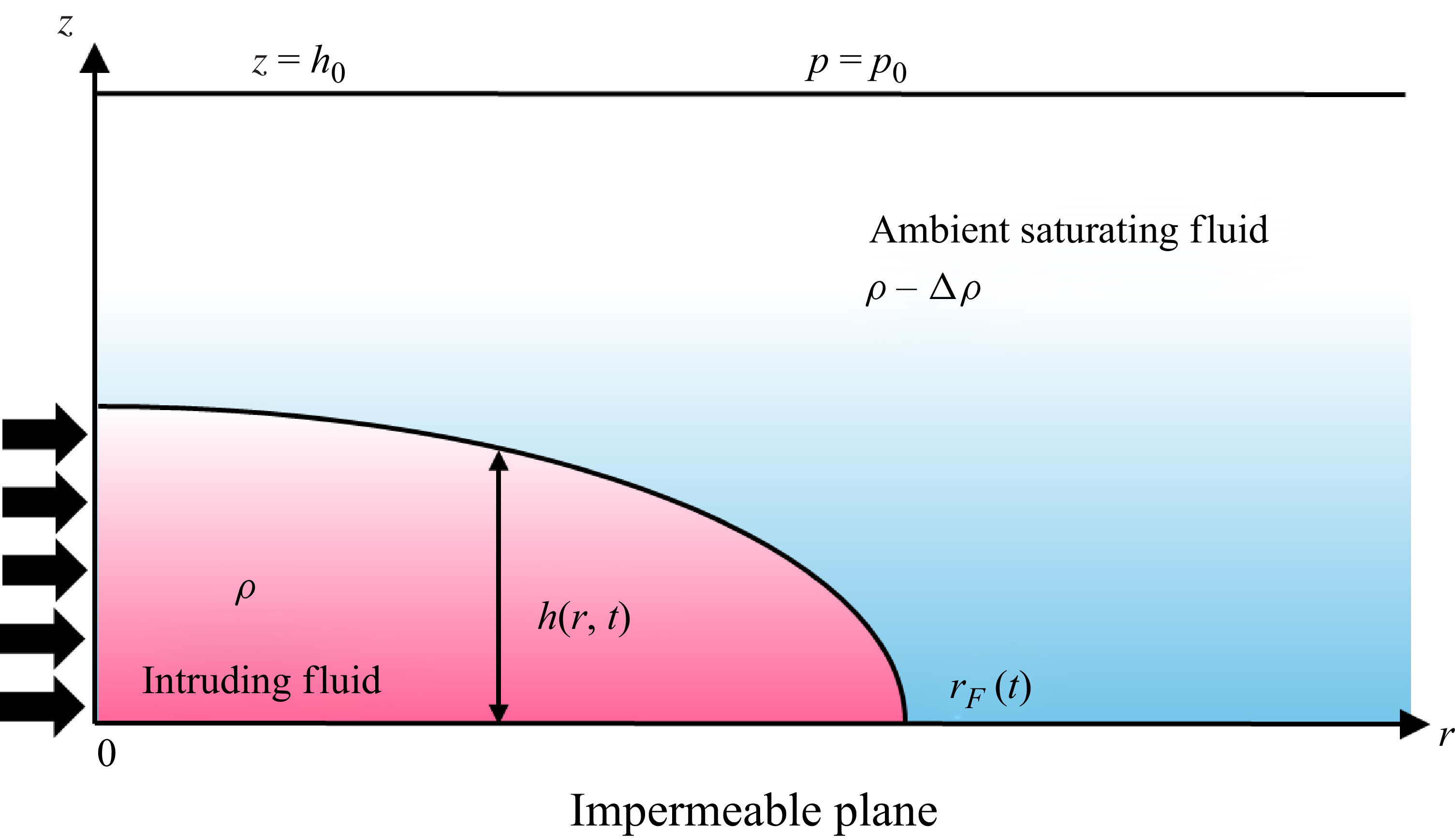
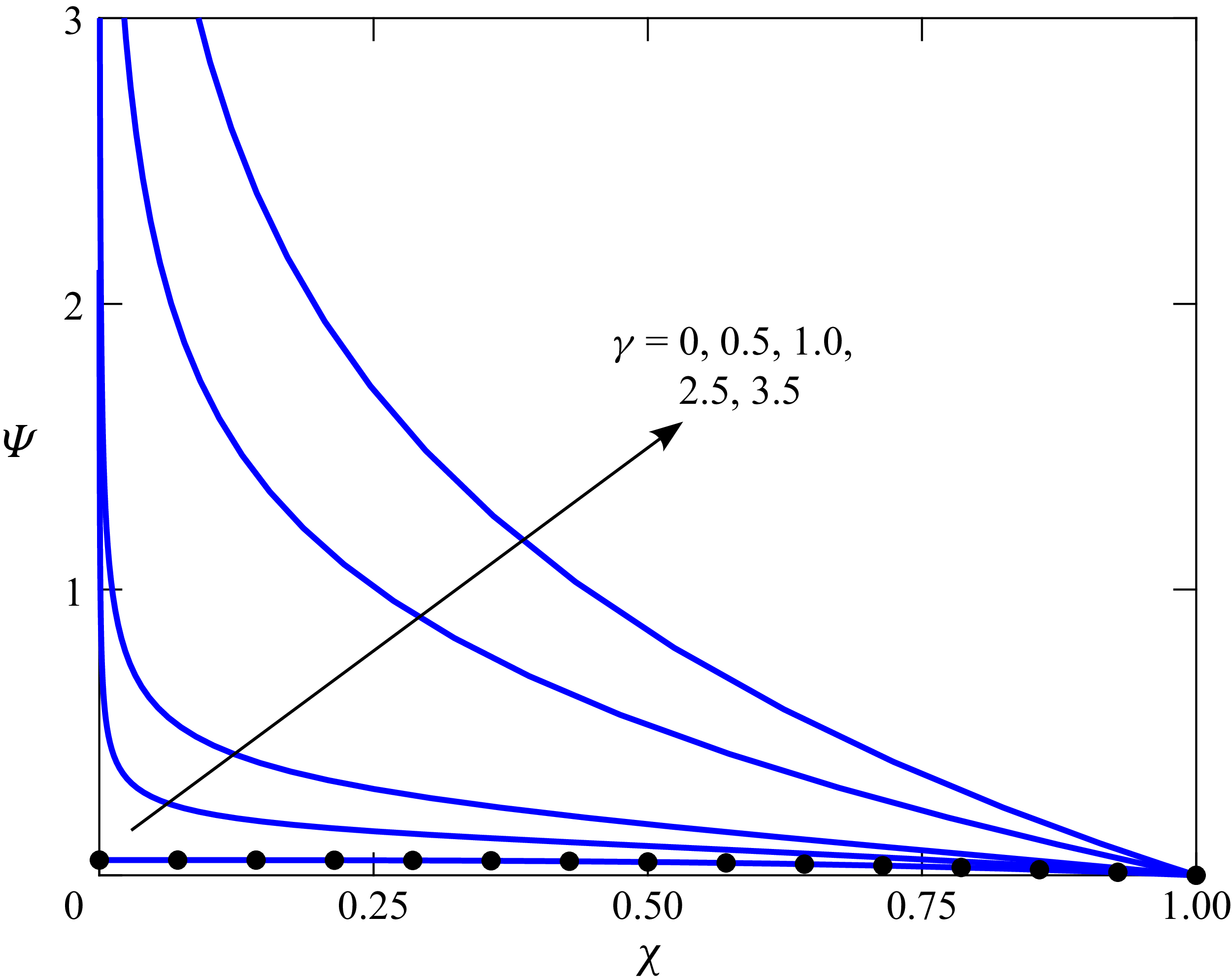
 Ψ
 χ
 γ
 γ=0
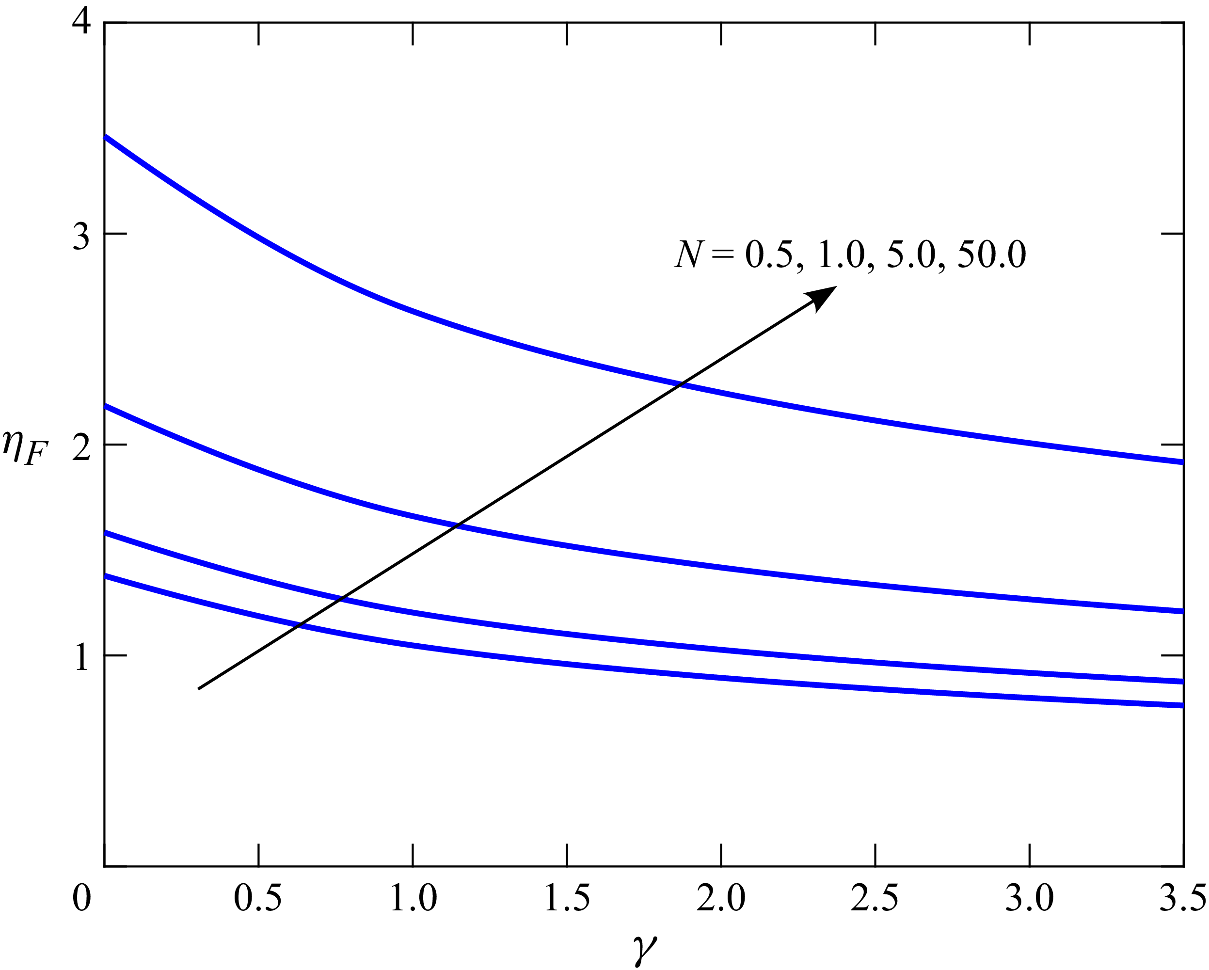
 ηF
 γ
 N

 N
 γ
 T=1,2,5,10,20
 T=1
 T=20
 N

 N
 γ=0
 γ=2.5
 ζ¯
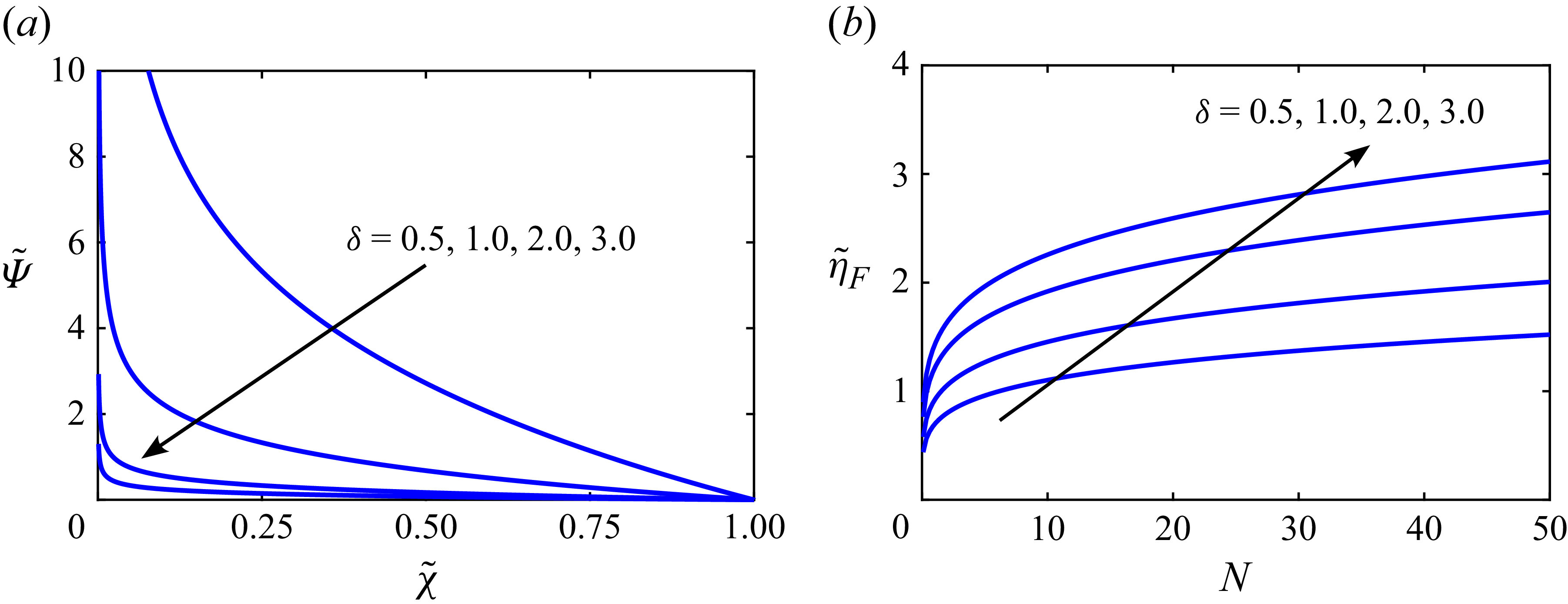
 Ψ~
 χ~
 η~F
 N
 γ=3
 δ
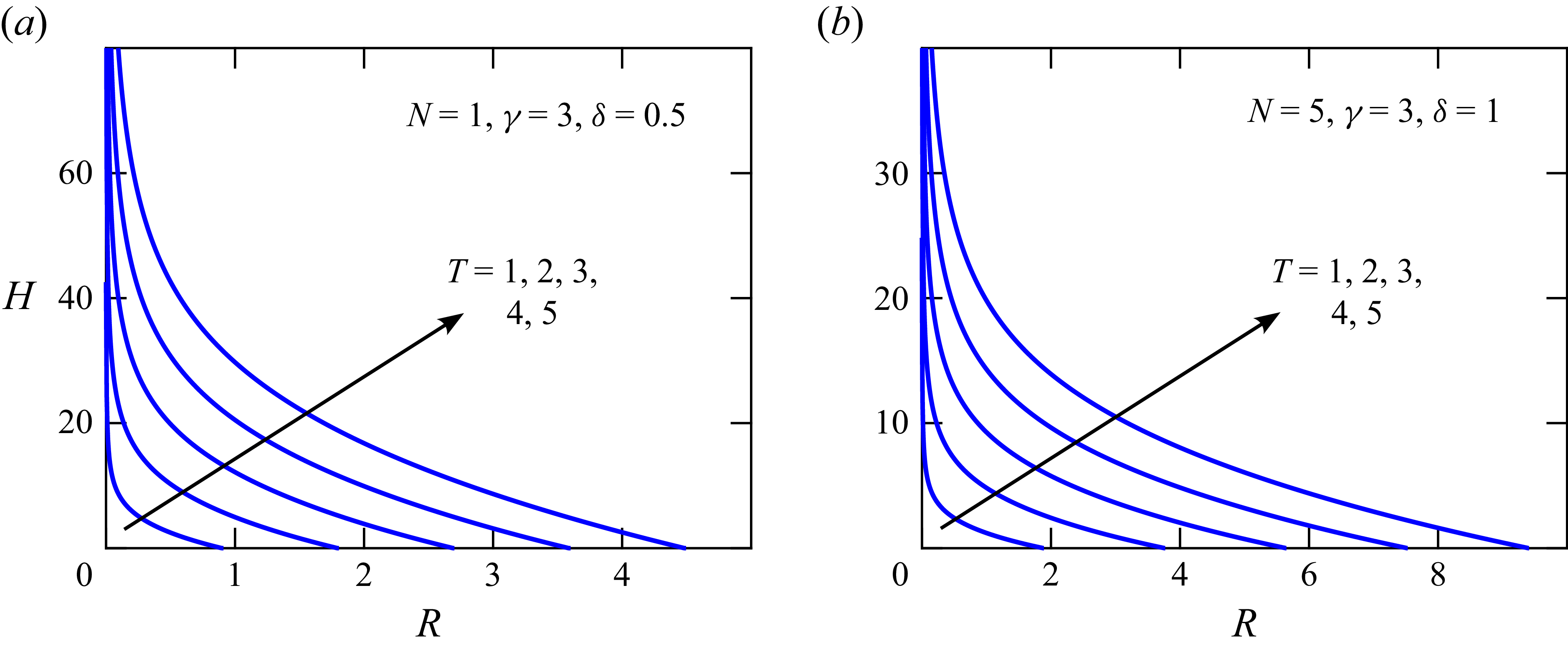
 γ=3
 N
 δ


 γ=0.3
 γ=1.5
 γ=3
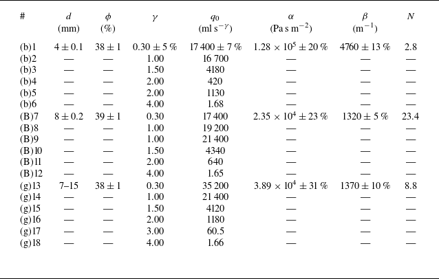
 d=4.0±0.1mm
 d=8±0.2mm
 d=7−15mm
 q0
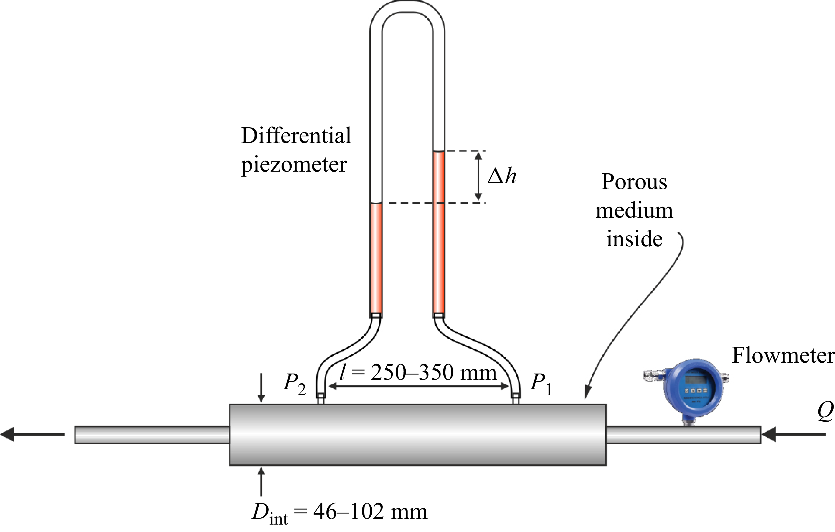
 α
 β

 α
 β
 d=4±0.1mm
 d=8±0.2mm
 7−15mm
 Δp/l=αu+ρβu2

 d=8

 d=4

 d=8

 d=7−15

 d=8
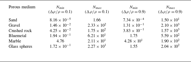
 N=(Δρ/ρ)g2bk2/ν2
 k
 b
 ν=1.337×10⁻⁶m2s−1

 N
 γ=3.5
 ζ¯
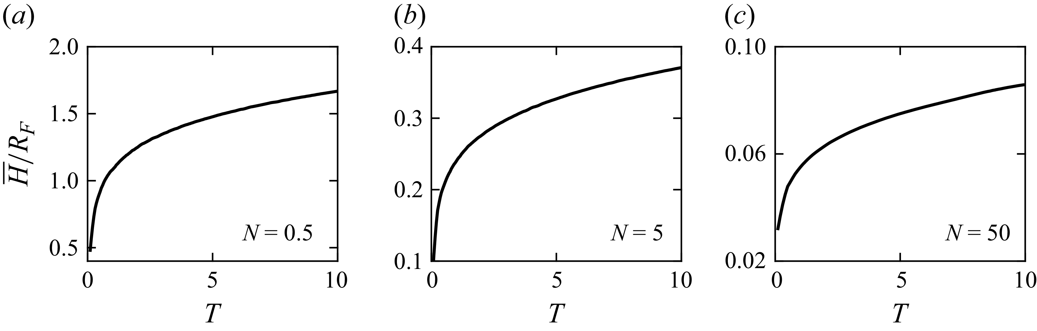
 H¯/RF
 N
 γ=3.5
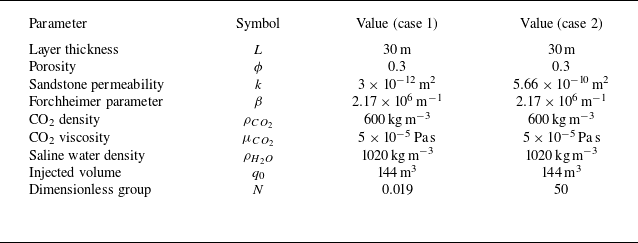
 CO2
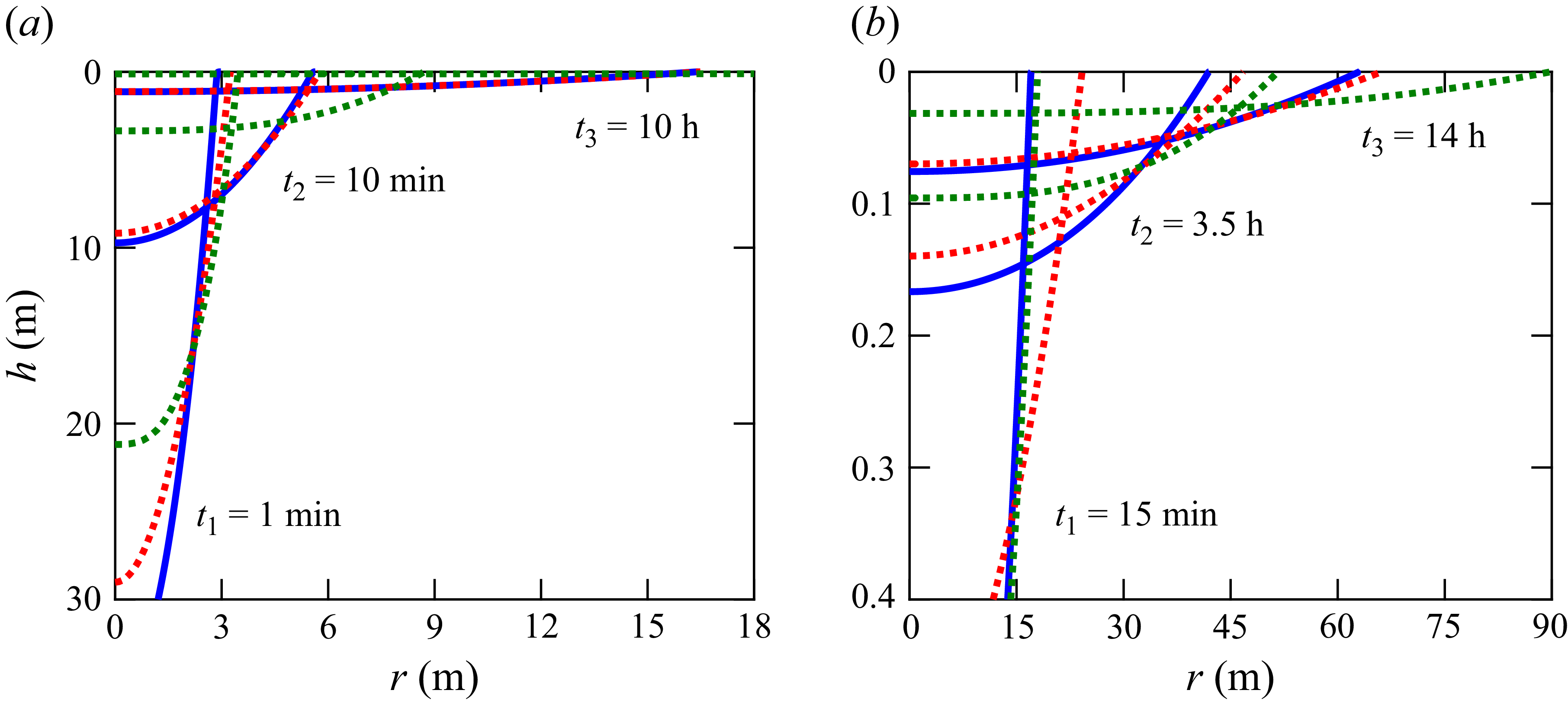
 CO2
 N=0.019
 N=50

 Open access

