Introduction

In glaciological field practice, surface motion is observed using standard surveying techniques or photogrammetry to measure the displacement of a survey stake or an identifiable surface feature. The expected errors in determining the initial and final positions are reported and are combined to give the expected error in the average velocity, which is computed by dividing the distance between the two positions by the elapsed time, and which is usually assigned to the point midway between the initial and final positions. A spatial distribution of velocity is constructed by interpreting the motion of several survey stakes or surface features in this way.

This method is susceptible to another source of error. The average velocity does not occur at the mid-point of its initial and final positions unless the actual velocity distribution belongs to a restricted class of mathematical functions. Recognizing this source of error may be helpful in reconciling observations of velocity and mass balance through the continuity equation.

The following is an elementary analysis of the case of steady, one-dimensional flow. Only the horizontal component of the longitudinal velocity is considered, and the transverse component is assumed to be zero. It is not necessary that the glacier be in steady state, that is with unchanging geometry, but only that the horizontal velocity distribution be unchanging over the time interval considered. Alternatively, if the actual velocity distribution is changing, the average velocity may be considered instead; it is defined to be a velocity distribution that, if it existed constantly over the time interval, would produce the observed displacements.

Using Particle Trajectories to get a Velocity Distribution

Where x is a horizontal coordinate that is positive in the direction of glacier flow, the velocity

of a particle is assumed to depend only on x; that is,

where g(x) is a positive, continuous function and ∂g(x)/∂t = 0. If the trajectory

gives the position of a particle on or near the surface at time t, and f(t) is a differentiable, increasing function, then, from Equations (1) and (3),

where f′(θ) ≡ df(θ)/dt. From Equation (3)

where f ⁻¹(θ) is the inverse of f(θ); that is, f ⁻¹[f(θ)] = f[f ⁻¹(θ)] = θ. Now, from Equations (2), (4), and (5),

Thus, if f(t) is known, g(x) is given by Equation (6).

Also, from Equations (1) and (2),

which is a first-order, ordinary differential equation easily integrated by separating variables

where x ₀ is the position of the particle at time t ₀. If

in which Γ is the constant of integration, then, from Equations (8) and (9),

or

where G ⁻¹[G(θ)] = G[G(θ)] = θ. Thus, if g(x) is known, f(t) is given by Equation (10).

As shown by Equation (6), the function x = f(t) must be known if the velocity distribution is to be determined; thus, knowing only the end-points (t ₀, x ₀) and (t ₁, x ₁) of a particle trajectory is insufficient for determining g(x). Moreover, as the trajectory end-points represent an integral of dx/dt = g(x), they do not determine any particular point on g(x), but rather they impose only an integral condition on it. Therefore, particular points on v = g(x) cannot be obtained from particle trajectory end-points.

The integral condition imposed on the velocity distribution by the trajectory end-points may be derived by introducing

and substituting for v in Equation (1) to get

which is directly integrated to yield

For the trajectory end-points (t ₀, x ₀) and (t ₁, x ₁),

Thus, in deducing a velocity distribution from a set of particle trajectory end-points, a function r(x) must be devised so that it obeys Equation (14) for each trajectory in the set (which in general may all have t ₀ and t ₁ different from one another, provided the assumption ∂g(x)/∂t = 0 holds throughout the entire combined time interval). Neither the time-averaged velocity nor the distance-averaged velocity is pertinent here; it is only the Equation (14) integral of the velocity reciprocal that satisfies the governing differential equation (7). The velocity distribution is not uniquely determined by the data because, through Equation (14), they impose conditions only on the integral of its reciprocal.

No doubt an optimizing algorithm could be developed that would construct an r(x) satisfying all the required integrals and also minimizing some measure of smoothness, such as the curvature-squared integral, so that the velocity distribution would be free from spurious features not implied by the data. A simple approach to constructing g(x) is first to fit a smooth curve to the ( x , v ) points from the several pairs of trajectory end-points used (see Equations (16) and (17)), and then to revise it iteratively until its reciprocal r(x) obeys Equation (14) for each pair of end-points.

After an r(x) has been constructed that is consistent with the end-point data, the velocity distribution is obtained easily from

Table 1 lists the end-points of the trajectories of three survey stakes and twelve surface features observed on the lower reach of Columbia Glacier, Alaska. Only the longitudinal component of position is given. Shown in Figure 1 is a numerically constructed r(x) representing the average velocity distribution over the period considered, for during this period there existed a pronounced seasonal variation (personal communication from M. F. Meier and others). The constructed r(x) is consistent with all fifteen trajectories, each of which is indicated by a horizontal line segment from x ₀ to x ₁ at r = Δt/Δx; each line segment has the integral required by Equation (14), It was constructed iteratively so that it agrees with the data of Table 1 and so that it is smooth, without any spurious features. The slight asynchronism of the fifteen time intervals is accommodated here by supposing that the same time-average velocity distribution exists throughout the entire combined intervals 25 August 1977 through 3 September 1978. The actual r(x) may have a deeper local minimum of r ≈ 1 a/km at x ≈ 26.5 km. Shown in Figure 2 is the velocity distribution v = g(x) = 1/r(x).

Table 1

Trajectory end-points for Three Survey Stakes and Twelve Photogrammetrically Observed Surface Features on the Lower Reach of Columbia Glacier

Fig. 1.

Reciprocal velocity function r(x) = 1/v constructed numerically to conform with the fifteen trajetories listed in Table 1.

Fig. 2.

Velocity distribution v = g(x), which is the reciprocal of the function shown in Figure 1.

The Trajectory-Average Method

Although the use of Equation (14) does not uniquely determine the velocity distribution, it does precisely express the entire influence that trajectory end-points have on it. Considered next is the error resulting from using the trajectory-average method to construct it. In this method, the average trajectory velocity

is assigned to g(x) at the trajectory mid-point

The error in assuming g( x ) = υ depends on what the actual velocity distribution is. From Equations (8) and (9)

and the relative error is

This is the error at x ; the error of the trajectory-average method as evaluated by Equation (14) depends on the way a continuous curve might be fitted through ( x , υ ) points calculated by that method from the end-points of several particle trajectories. In investigating the error at x , the choice of functional forms for g(x) is restricted to those amenable here to manipulation through equations (1) to (10). In each of the three special cases considered, a simple mathematical form for g(x) is assumed, and closed-form expressions are obtained for the trajectory f(t) and the relative error E. The complication that sometimes occurs for the coefficients of g(x) and f(t) arises from requiring f(t) to agree with the trajectory end-points.

First considered is the case in which g(x) is a linear function of x. It is parametrized by the ratio a of the velocities at x ₀ and x ₁; that is, g(x ₁)/g(x ₀) = a. The relevant equations are, for a ≠ 1,

and

and the relative error is

which is negative for all non-zero gradients dv/dx = (ln a)/Δt. In the trivial a = 1 case: g(x) = υ , f(t) = x ₀ + (t – t ₀) υ , and E ₁ = 0. Because E ₁(a) is an even function of ln a, it depends only on the magnitude of the gradient, not on its direction. It is shown as Figure 3; it approaches −1 as a goes to infinity or zero, and it has an inflection point at E ₁(2.169) = −0.047 1. In Figure 4 are shown f(t) for selected a.

Fig. 3.

Relative error E ₁(a) for linear velocity distribution v = g(x) where a = g(x ₁)/g(x ₀).

Fig. 4.

Particle trajectories x = f(t) from linear velocity distributions v = g(x) for a = g(x ₁)/g(x ₀) as indicated.

That E ₁(a) is independent of the direction of the velocity gradient is a special case of the independence, for any g(x), of the relative error at x from the direction in which a particle traverses a feature of g(x); that is, the relative error at x is unchanged if g(x) is reflected about x = x . This is easily established by setting , from which 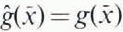and, from Equation (9)

so that, from Equation (19),

Second is considered the case of a velocity extremum in which g(x) is taken to be a quadratic function of x. It is parameterized by the ratio b of the velocity at the mid-point to the velocity at the end-points; that is, g( x )/g(x ₀) = g( x )/g(x ₁) = b. The velocity distribution is

Defining

the value of g( x ) that is consistent with the trajectory end-points

the trajectory is

and the relative error is

Figure 5 shows g(x)/g(x ₀) for selected b, and Figure 6 gives the corresponding f(t). Figure 7 gives E ₂(b) as the solid curve.

Fig. 5.

Quadratic velocity distributions v = g(x) for b = g( x )/g(x ₀) as indicated.

Fig. 6.

Particle trajectories x = f(t) from quadratic velocity distributions v = g(x), for b = g( x )/g(x ₀) as indicated.

Fig. 7.

Relative error, E ₂(b) for quadratic velocity distribution (solid curve) and E ₃(c) for conic velocity distribution (dashed curve), where v = g(x) and b, c = g( x )/g(x ₀).

Third is considered another form for a velocity extremum in which g(x) is taken to be a segment of a conic section. This functional form is included because the form of Equation (24) does not span all second-degree possibilities. It is parameterized by the ratio c of the velocity at the mid-point to the velocity at the end-points; that is, g( x )/g(x ₀) = g( x )/g(x ₁) = b. The velocity distribution is

Defining

the value of g( x ) that is consistent with the trajectory end-points is

the trajectory is

and the relative error is

When c > 1 the conic is an ellipse, and when c < 1 it is a hyperbola. Figure 8 shows g(x)/g(x ₀) for selected c, and Figure 9 gives the corresponding f(t). Figure 7 gives E ₃(c) as the dashed curve.

Fig. 8.

Conic velocity distributions v = g(x) for c = g( x )/g(x ₀) as indicated.

Fig. 9.

Particle trajectories x = f(t) from conic velocity distributions v = g(x), for c = g( x )/g(x ₀) as indicated.

Although it is difficult to determine the error in assigning ( x , υ ) to g(x) for arbitrary g(x), it is easy to determine the class of functions to which g(x) must belong if g( x ) = υ . Equation (14) may be written

where . Since any function can be expressed as the sum of an odd function and an even function, let

where , from which 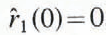, and . If g( x ) = υ , then , and Equation (34) may be written

Because the first integral vanishes identically and the third integral is Δx/ υ = Δt, the second integral must also vanish; this gives the other condition on the velocity distribution for it to include ( x , υ ). The simplest form for such g(x) then is 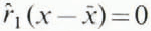and , which gives g( x ) = υ . This is the trivial case with zero gradient of the linear, quadratic, and conic functions examined above for g(x). Increasing the degree of r(x) by one gives

where s is a constant, which is a hyperbola with gradient dv/dx = −sv ².

Equation (37) can be interpreted glaciologically if it is assumed that the glacier flux Q obeys

where h(x) is the glacier thickness and F is a constant, and if it is assumed that over some x-interval Q is also constant and h(x) is linear, then over that interval g(x) has the same form as in Equation (37) and g( x ) = υ . In fact, the conditions on Q and F can be relaxed slightly; Q and F can both vary with x as long as the ratio Q(x)/F(x) is constant. This special case, however, should not be embraced as a basis for neglecting the error to which the trajectory-average method is susceptible; in spite of this effect, the curves of Figures 3 and 7 still exhibit errors of several per cent, and so does the actual glacier velocity distribution discussed next. It is mentioned only to put Equation (37) into a glaciological context, not to suggest that the conditions occur in actual glaciers with any particular frequency.

An actual glacier velocity distribution provides another example of the error in the trajectory-average method. The velocity distribution for the ice-fall reach of Columbia Glacier (from unpublished data taken in 1982 by M. F. Meier and others) is shown as the solid curve in Figure 10; it is much more complex than the one for the lower reach shown in Figure 2. If the velocity distribution is assumed to be unchanging from time t ₀ until time t ₁ = t ₀ + Δt, then for a survey stake initially at some position x ₀, its final position x ₁ is given by Equation (14); the average trajectory velocity, given by equation (16), is assigned to the trajectory mid-point, given by Equation (17). If a dense array of hypothetical survey stakes were assumed to exist at time t ₀, and if the solid curve in Figure 10 is assumed to be the actual velocity distribution, then the velocity distribution that would be produced by the trajectory-average method can be developed: the dashed curve in Figure 10 is the distribution so developed for one year Δt. The relative error E, which is given by Equation (19), can also be computed at the mid-point of the trajectory of each hypothetical stake; the E(x) for the dashed curve in Figure 10 is shown as the dashed curve in Figure 11, which also gives the E(x) for Δt = 2.0, 0.5, and 0.25 a.

Fig. 10.

Velocity distribution for the ice-fall reach of the Columbia Glacier, both the actual (solid curve) and that which would be produced by the trajectory-average method (dashed curve).

Fig. 11.

Relative error E(x) in applying the trajectory-average method to the velocity distribution shown as the solid curve in Figure 10 for Δt = 2.0a (solid curve), 1.0a (dashed curve), 0.5a (dotted curve), and 0.25a (crossed curve).

Several conclusions can be drawn from this actual case. First, the velocity distribution arising from the trajectory-average method is one that yields a subdued curve, especially in its understatement of the extrema; however, the extreme values of the associated error distribution are displaced from those extrema (compare the dashed curves in Figures 10 and 11). Second, at any x, the error is roughly proportional to Δt. Third, the error cannot be avoided or reduced by some stake placement technique, because this case has been analyzed by assuming a continuum of hypothetical stakes, although a very sparse stake spacing could fail entirely to detect features in the velocity distribution. Therefore, if a field program is to be designed to reduce the error in using the trajectory-average method, only shortening the period between position measurements will have any effect, not the stake placement pattern. The error depends only on the actual velocity distribution a stake traverses in a particular time Δt, not on the position of some other stake. Easier than shortening the measurement period would be using Equation (14) in the construction of the velocity distribution, rather than using the trajectory-average method.

Summary

The trajectory end-points customarily observed in glacier field programs impose only an integral condition on the velocity distribution. Therefore, they do not uniquely determine it, or any individual points on it.

The trajectory-average method, in which the average trajectory velocity υ is assigned to the trajectory mid-point x , has an inherent error. For a one-year interval Δt between position measurements, this error can reach several per cent for velocity distribution features that are typical of actual glaciers. The case of the ice-fall reach of Columbia Glacier suggests that this error is roughly proportional to Δt.

The only field program tactic that can be used to reduce this error is to shorten Δt. Although spatially enriching a stake array will give more information about the velocity distribution, it cannot reduce this error.

The ( x , υ ) points are useful in making a first approximation to the velocity distribution. The reciprocal of a smooth curve through them should be revised as necessary to make it obey Equation (14) for all trajectory end-points used. The reciprocal of this revised reciprocal curve is then the velocity distribution.