1 Introduction and motivation
Modelling turbulent boundary layers (TBL) has been an increasingly active area of research, leading to proposals of various reduced-order as well as conceptual models. Amongst the latter, the attached eddy model that has evolved from the attached eddy hypothesis (AEH) of Townsend (Reference Townsend1976) is well known and provides a kinematic description of the logarithmic (log) region of wall turbulence. It assumes the TBL as an assemblage of randomly distributed geometrically self-similar attached eddies or structures, with their population density inversely proportional to their size (see Marusic & Monty (Reference Marusic and Monty2019) for a comprehensive review). Throughout this article, the words ‘structures’, ‘eddies’ and ‘motions’ are used interchangeably and essentially refer to the definition of a coherent eddy given by Robinson (Reference Robinson1991). Coherent eddies can be self-similar or non-self-similar (Perry, Henbest & Chong Reference Perry, Henbest and Chong1986; Perry & Marusic Reference Perry and Marusic1995). A self-similar eddy refers to a flow structure whose geometric lengths and velocity field scale with distance from the wall ( $z$) and friction velocity (
 $U_{\unicode[STIX]{x1D70F}}$), respectively. A non-self-similar eddy, on the other hand, does not exhibit these characteristics.
Based on the attached eddy model, Perry et al. (Reference Perry, Henbest and Chong1986) showed using spectral-overlap arguments that self-similarity leads to a  $k_{x}^{-1}$ scaling in the premultiplied one-dimensional (1-D)
 $u$-spectra. Here,
 $k_{x}$ is the streamwise wavenumber and
 $u$,
 $v$ and
 $w$ would refer to the streamwise, spanwise and wall-normal velocity fluctuations respectively, associated with the coordinate system
 $x$,
 $y$ and
 $z$. However, the true
 $k_{x}^{-1}$ scaling for the
 $u$-spectra, representative of the contributions from purely self-similar eddies has been obscured in the previously reported experiments and simulations due to various reasons, namely: (i) spectral aliasing (Davidson, Nickels & Krogstad Reference Davidson, Nickels and Krogstad2006; Chandran et al. Reference Chandran, Baidya, Monty and Marusic2017) and (ii) overlapping contributions from various eddy types at finite
 $Re_{\unicode[STIX]{x1D70F}}$ (Perry et al. Reference Perry, Henbest and Chong1986; Perry & Marusic Reference Perry and Marusic1995; Baars & Marusic Reference Baars and Marusic2020). The present study tests the notion of self-similarity by bypassing both the aforementioned scenarios through a methodology discussed ahead.
The 1-D spectra represents the average energy contribution over the entire range of  $k_{y}$, for a particular
 $k_{x}$, making it susceptible to spectral aliasing (Tennekes & Lumley Reference Tennekes and Lumley1972). In that respect, a better alternative to the 1-D
 $u$-spectrum is the direct measurement of the 2-D
 $u$-spectrum as a function of both
 $k_{x}~(=2\unicode[STIX]{x03C0}/\unicode[STIX]{x1D706}_{x})$ and
 $k_{y}~(=2\unicode[STIX]{x03C0}/\unicode[STIX]{x1D706}_{y})$. The 2-D spectrum, however, is difficult to measure experimentally at high
 $Re_{\unicode[STIX]{x1D70F}}$. Chandran et al. (Reference Chandran, Baidya, Monty and Marusic2017) were able to measure 2-D
 $u$-spectra at
 $2400\lesssim Re_{\unicode[STIX]{x1D70F}}\lesssim 26\,000$, in the log-region of a zero pressure gradient (ZPG) TBL, by first reconstructing the 2-D two-point correlation:
 $$\begin{eqnarray}\left.\begin{array}{@{}c@{}}R_{u_{o}u_{r}}(\unicode[STIX]{x0394}x,\unicode[STIX]{x0394}y;z_{o},z_{r})=\overline{u(x,y,z_{r})u(x+\unicode[STIX]{x0394}x,y+\unicode[STIX]{x0394}y,z_{o})},\\ \text{with}~\widetilde{{\mathcal{R}}}_{u_{o}u_{r}}=R_{u_{o}u_{r}}/(\sqrt{u^{2}(z_{o})}\sqrt{u^{2}(z_{r})}).\end{array}\right\}\end{eqnarray}$$
Subsequently, the 2-D spectrum was computed by taking the 2-D Fourier transformation of  $R_{u_{o}u_{r}}$ as:
 $$\begin{eqnarray}\unicode[STIX]{x1D719}_{u_{o}u_{r}}(k_{x},k_{y};z_{o},z_{r})=\iint _{-\infty }^{\infty }R_{u_{o}u_{r}}(\unicode[STIX]{x0394}x,\unicode[STIX]{x0394}y;z_{o},z_{r})\text{e}^{-j2\unicode[STIX]{x03C0}(k_{x}\unicode[STIX]{x0394}x+k_{y}\unicode[STIX]{x0394}y)}\,\text{d}(\unicode[STIX]{x0394}x)\,\text{d}(\unicode[STIX]{x0394}y),\end{eqnarray}$$
where  $j$ is a unit imaginary number and overbar denotes ensemble time average. Throughout this article, the 2-D spectrum refers to the modulus of the premultiplied form of
 $\unicode[STIX]{x1D719}_{u_{o}u_{r}}$ normalized by the friction velocity (i.e.
 $|k_{x}^{+}k_{y}^{+}\unicode[STIX]{x1D719}_{u_{o}u_{r}}/U_{\unicode[STIX]{x1D70F}}^{2}|$). For convenience, the 2-D spectrum for
 $z_{r}=z_{o}$ will be referred to as
 $\unicode[STIX]{x1D6F7}$, while that for
 $z_{r}\neq z_{o}$ will be referred to as
 $\unicode[STIX]{x1D6F7}_{cross}$. In agreement with del Alamo et al. (Reference del Alamo, Jiménez, Zandonade and Moser2004), at
 $Re_{\unicode[STIX]{x1D70F}}\approx 2400$, Chandran et al. (Reference Chandran, Baidya, Monty and Marusic2017) observed the constant-energy region of
 $\unicode[STIX]{x1D6F7}$ to be nominally bounded by power laws
 $\unicode[STIX]{x1D706}_{y}/z_{o}\sim (\unicode[STIX]{x1D706}_{x}/z_{o})^{1/2}$ in the large-scale range:
 $\unicode[STIX]{x1D706}_{x}/z_{o},\unicode[STIX]{x1D706}_{y}/z_{o}>10$. Here, the wavelengths
 $\unicode[STIX]{x1D706}_{x}$ and
 $\unicode[STIX]{x1D706}_{y}$ were interpreted as the surrogate length and width of the energetic eddies in the TBL. Therefore, the observation of a square-root relationship suggested a failure of self-similarity at low
 $Re_{\unicode[STIX]{x1D70F}}$ since it indicates that the eddies do not grow wider (with
 $z$) at the same rate as they grow longer. At
 $Re_{\unicode[STIX]{x1D70F}}\approx 26\,000$, however, they found that the large scales deviate from the square-root relationship towards a linear behaviour (
 $\unicode[STIX]{x1D706}_{y}/z_{o}\sim \unicode[STIX]{x1D706}_{x}/z_{o}$), which is representative of the self-similarity. The large-scale range where this change occurs was referred to as the large-eddy region, existing in the nominal range
 $\unicode[STIX]{x1D706}_{x}>10z_{o}$ and
 $\unicode[STIX]{x1D706}_{x}<7\unicode[STIX]{x1D6FF}$ (Chandran et al. Reference Chandran, Baidya, Monty and Marusic2017; Chandran Reference Chandran2019).
Chandran et al. (Reference Chandran, Baidya, Monty and Marusic2017) conjectured that clear evidence of self-similarity would be observed only for a TBL at  $Re_{\unicode[STIX]{x1D70F}}\gtrsim 60\,000$, due to
 $\unicode[STIX]{x1D6F7}(z_{o})$ comprising energy contributions from various eddy types existing at
 $z_{o}$, which obey different scalings (Baars & Marusic Reference Baars and Marusic2020). These contributions overlap with one another at relatively lower
 $Re_{\unicode[STIX]{x1D70F}}$ (
 ${\lesssim}60\,000$), due to the limited scale separation, obscuring any
 $\unicode[STIX]{x1D706}_{y}/z_{o}\sim \unicode[STIX]{x1D706}_{x}/z_{o}$ relationship that may be present. The issue relates to the second reason ((ii) mentioned above) responsible for obscuring self-similar trends in previous studies, and we attempt to resolve it here by ‘filtering’ out the energy contribution from the non-self-similar structures to bring out the self-similarity unequivocally. Here, the term ‘filter’ is used to refer, in general, the methodology adopted to extract flow statistics at
 $z_{o}$ contributed by structures coherent across a specified wall-normal range, say
 $z_{r}$–
 $z_{o}$. Different studies have adopted different approaches to ‘filter’ out these non-self-similar contributions, with some making use of the wall filter. Here, the prefix ‘wall’ before ‘filter’ refers to the methodology utilized for extracting flow features (at
 $z_{o}$) contributed by eddies extending all the way down to the wall (
 $z_{r}\rightarrow 0$). These are referred to as the wall-attached structures in the present manuscript. Similarly, structures which physically do not extend to the wall will be referred as wall-detached structures.
Two recent studies, utilizing the wall filter, have shown promising results with respect to removing the non-self-similar contributions. The first is by Hwang & Sung (Reference Hwang and Sung2018), who following the works of del Alamo et al. (Reference del Alamo, Jiménez, Zandonade and Moser2004) and Lozano-Durán, Flores & Jiménez (Reference Lozano-Durán, Flores and Jiménez2012), implemented a wall filter in their instantaneous ZPG TBL DNS fields at  $Re_{\unicode[STIX]{x1D70F}}\approx 1000$ to extract only those energetic motions which were physically attached to the wall. Analysis of these filtered fields revealed a linear relationship between the streamwise and spanwise length scales for the large wall-attached structures. This evidence led them to conclude that the extracted structures were principal candidates for Townsend’s AEH. The structures from the
 $Re_{\unicode[STIX]{x1D70F}}\approx 1000$ DNS, however, are likely not statistically dominant in the log-region due to an insufficient scale separation (Hwang & Sung Reference Hwang and Sung2018), encouraging a similar analysis at higher
 $Re_{\unicode[STIX]{x1D70F}}$. The second study, by Baars, Hutchins & Marusic (Reference Baars, Hutchins and Marusic2017), involved computing the 1-D linear coherence spectrum from synchronized two-point
 $u$-signals acquired at a near-wall and log-region reference location. They identified the characteristic lengths of the energetic wall-attached structures to be scaling self-similarly with
 $z_{o}$, as
 $\unicode[STIX]{x1D706}_{x}/z_{o}\approx 14$. The analysis, which spanned datasets across three decades of
 $Re_{\unicode[STIX]{x1D70F}}$, led to the conclusion that a ‘self-similar attached eddy structure is ingrained within the TBL flow’. Agostini & Leschziner (Reference Agostini and Leschziner2017) made similar observations for structures in the mesolayer. The present study may be viewed as a first step towards the extension of the work by Baars et al. (Reference Baars, Hutchins and Marusic2017) to the 2-D scenario. Here, we study the 2-D cross-spectrum,
 $\unicode[STIX]{x1D6F7}_{cross}^{w}$ (i.e.
 $z_{r}\neq z_{o}$; superscript ‘
 $w$’ used when
 $z_{r}^{+}\lesssim 15$) by considering
 $z_{r}$ in the near-wall region and
 $z_{o}$ in the log-region. Therefore,
 $\unicode[STIX]{x1D6F7}_{cross}^{w}(z_{o},z_{r})$ shows the 2-D distribution of energy contributed purely by the wall-attached eddies that extend up to
 $z_{o}$ and beyond (with
 $z_{o}\gg z_{r}$), and is investigated here to test the notion of self-similarity. Throughout the article, superscript ‘+’ indicates normalization by viscous length (
 $\unicode[STIX]{x1D708}/U_{\unicode[STIX]{x1D70F}}$) and velocity (
 $U_{\unicode[STIX]{x1D70F}}$) scales.
2 Experimental and numerical data
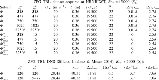
Two TBL datasets across a decade of  $Re_{\unicode[STIX]{x1D70F}}$ are considered for analysis in the present study (table 1). The high-
 $Re_{\unicode[STIX]{x1D70F}}$ dataset (
 ${\mathcal{E}}_{1}$) includes 2-D
 $u$-spectra (
 $\unicode[STIX]{x1D6F7}$) and first measurements of 2-D
 $u$-cross-spectra (
 $\unicode[STIX]{x1D6F7}_{cross}^{w}$) at
 $Re_{\unicode[STIX]{x1D70F}}\approx 15\,000$. This dataset was obtained via synchronized multipoint hot-wire measurements in the large Melbourne wind tunnel (HRNBLWT) and the details of these experiments are provided in table 1. Here,
 $l$,
 $U_{\infty }$ and
 $T$ denote the hot-wire sensor length, free-stream velocity and total sampling duration, respectively. Boundary layer thickness,
 $\unicode[STIX]{x1D6FF}$, and the friction velocity,
 $U_{\unicode[STIX]{x1D70F}}$, are estimated via the composite fit proposed by Chauhan, Monkewitz & Nagib (Reference Chauhan, Monkewitz and Nagib2009).
 $2.5~\unicode[STIX]{x03BC}\text{m}$ diameter Wollaston hot-wire probes were used for all measurements, which were operated using an in-house Melbourne University Constant Temperature Anemometer at a rate of
 $\unicode[STIX]{x0394}T^{+}\equiv U_{\unicode[STIX]{x1D70F}}^{2}/(\unicode[STIX]{x1D708}f_{s})\approx 0.5$, where
 $f_{s}$ refers to sampling frequency.
A summary of the various datasets containing synchronized multipoint  $u$-signals at
 $z_{r}$ and
 $z_{o}$ for various spanwise offsets,
 $\unicode[STIX]{x0394}y$. Terminology has been described in § 2. Values highlighted in bold indicate the approximate
 $z^{+}$-location for the beginning of the log-region,
 $2.6\sqrt{Re_{\unicode[STIX]{x1D70F}}}$ (Klewicki, Fife & Wei Reference Klewicki, Fife and Wei2009), underlined represent
 $z^{+}\approx 3.9\sqrt{Re_{\unicode[STIX]{x1D70F}}}$ and the ones with superscript (*) represent the upper limit of the log-region,
 $z^{+}\approx 0.15\unicode[STIX]{x1D6FF}^{+}$ (Marusic et al. Reference Marusic, Monty, Hultmark and Smits2013).

First, two-point measurements with  $z_{r}^{+}\approx z_{o}^{+}$ were conducted with the aim to obtain
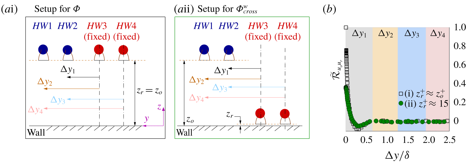
 $\unicode[STIX]{x1D6F7}$ at five wall-normal locations in the log-region, by employing the same experimental set-up and methodology used by Chandran et al. (Reference Chandran, Baidya, Monty and Marusic2017). Figure 1(ai) shows the schematic of the experimental set-up used to reconstruct the corresponding
 $R_{u_{o}u_{r}}$, with four hot-wire probes (
 $HW1$–
 $4$) located at
 $z_{o}$. Following the calibration procedure adopted by Chandran et al. (Reference Chandran, Baidya, Monty and Marusic2017),
 $HW1$,
 $HW2$ and
 $HW4$ were calibrated at
 $z_{o}$ by using the free-stream calibrated
 $HW3$ as reference. During experiments,
 $HW3$ and
 $HW4$ remained stationary at a fixed spanwise location while
 $HW1$ and
 $HW2$ were traversed together in the spanwise direction with logarithmic spacing.
 $u$-velocity time series acquired from a pair of hot wires are cross-correlated to obtain the correlation coefficient (
 $\widetilde{{\mathcal{R}}}_{u_{o}u_{r}}$) as a function of the spanwise spacing
 $\unicode[STIX]{x0394}y$ (figure 1b). At the start of the measurement,
 $HW2$ and
 $HW3$ were kept as close as practicably possible, at
 $(\unicode[STIX]{x0394}y_{1})_{min}\approx 0.01\unicode[STIX]{x1D6FF}$. Thereafter, every step movement of the traverse gives
 $\widetilde{{\mathcal{R}}}_{u_{o}u_{r}}$ at four distinct spanwise spacings:
 $\unicode[STIX]{x0394}y_{1}$ (
 $HW2$–
 $HW3$),
 $\unicode[STIX]{x0394}y_{2}$ (
 $HW1$–
 $HW3$),
 $\unicode[STIX]{x0394}y_{3}$ (
 $HW2$–
 $HW4$) and
 $\unicode[STIX]{x0394}y_{4}$ (
 $HW1$–
 $HW4$). Figure 1(b) highlights the
 $\unicode[STIX]{x0394}y$ range covered by each of these hot-wire pairs with different background colours. The experiment continues up to
 $(\unicode[STIX]{x0394}y_{4})_{max}\approx 2.7\unicode[STIX]{x1D6FF}$, enabling computation of
 $\widetilde{{\mathcal{R}}}_{u_{o}u_{r}}$ for
 $\unicode[STIX]{x0394}y=0$ and
 $(\unicode[STIX]{x0394}y_{1})_{min}\leqslant \unicode[STIX]{x0394}y\leqslant (\unicode[STIX]{x0394}y_{4})_{max}$. Taylor’s hypothesis, with the mean streamwise velocity at
 $z_{o}$ considered as the convection velocity, is employed to construct
 $\widetilde{{\mathcal{R}}}_{u_{o}u_{r}}$ at different streamwise spacings (
 $\unicode[STIX]{x0394}x$) for the temporal dataset,
 ${\mathcal{E}}_{1}$.
 $\unicode[STIX]{x1D6F7}(z_{o})$ is finally obtained from
 $R_{u_{o}u_{r}}$ via (1.2). It should be noted that
 $(\unicode[STIX]{x0394}y_{1})_{min}$ is limited to
 $0.01\unicode[STIX]{x1D6FF}$ for the set-up in figure 1(ai), which leads to energy redistribution in
 $\unicode[STIX]{x1D6F7}$ at small spanwise scales (Chandran et al. Reference Chandran, Baidya, Monty and Marusic2017). To account for this, the DNS-based correction scheme proposed by Chandran et al. (Reference Chandran, Baidya, Monty and Marusic2016) has been implemented to correct
 $\unicode[STIX]{x1D6F7}$ using the 2-D
 $\widetilde{{\mathcal{R}}}_{u_{o}u_{r}}$ obtained from the dataset of Sillero et al. (Reference Sillero, Jiménez and Moser2014).
(a) Schematic of the experimental set-up in HRNBLWT showing relative positioning and movement of the four hot-wire probes ( $HW1$–
 $HW4$) for reconstructing the 2-D correlation corresponding to (i)
 $\unicode[STIX]{x1D6F7}$ and (ii)
 $\unicode[STIX]{x1D6F7}_{cross}^{w}$. Mean flow direction is along
 $x$. (b) Correlation coefficients (
 $\widetilde{{\mathcal{R}}}_{u_{o}u_{r}}$) as a function of spanwise separation
 $\unicode[STIX]{x0394}y/\unicode[STIX]{x1D6FF}$, computed for
 $z_{o}^{+}\approx 2.6\sqrt{Re_{\unicode[STIX]{x1D70F}}}$ and
 $\unicode[STIX]{x0394}x=0$.

To obtain  $R_{u_{o}u_{r}}$ corresponding to
 $\unicode[STIX]{x1D6F7}_{cross}^{w}$,
 $HW3$ and
 $HW4$ were fixed at
 $z_{r}^{+}\approx 15$ while
 $HW1$ and
 $HW2$ were positioned at the same
 $z_{o}^{+}$ (figure 1aii) as in the measurements for
 $\unicode[STIX]{x1D6F7}$. Since the wall-coherence analysis remains largely unaffected for
 $0\leqslant z_{r}^{+}\lesssim 15$ (Baars et al. Reference Baars, Hutchins and Marusic2017), the positioning of the wall-reference probe at
 $z_{r}^{+}\approx 15$ was considered appropriate. Except for the difference in the wall-normal locations of
 $HW3$ and
 $HW4$, the measurement technique to compute
 $R_{u_{o}u_{r}}$ is similar to the previous case. However, for this set-up,
 $(\unicode[STIX]{x0394}y_{1})_{min}$ was reduced to zero by vertically aligning
 $HW2$ above
 $HW3$. The 1-D linear coherence spectrum (Baars et al. Reference Baars, Hutchins and Marusic2017) computed from the
 $u$-signals acquired by these two probes, at
 $\unicode[STIX]{x0394}y_{1}\approx 0$, agreed with its empirical fit proposed by Baars et al. (Reference Baars, Hutchins and Marusic2017), confirming the vertical alignment. Hence, as opposed to
 $\unicode[STIX]{x1D6F7}$, no small-scale correction was required for
 $\unicode[STIX]{x1D6F7}_{cross}^{w}$. A part of this dataset has also been used recently by Deshpande, Monty & Marusic (Reference Deshpande, Monty and Marusic2019), wherein the sensitivity of the 1-D linear coherence spectrum to
 $\unicode[STIX]{x0394}y$ has been showcased.
The low- $Re_{\unicode[STIX]{x1D70F}}$ dataset (
 ${\mathcal{S}}_{1}$) considered in the present study is that of Sillero et al. (Reference Sillero, Jiménez and Moser2014). Thirteen raw DNS time blocks are considered, each of which is a subset of the full computational domain between
 $x_{start}$ and
 $x_{end}$ (see table 1) to ensure a limited
 $Re_{\unicode[STIX]{x1D70F}}$ increase along
 $x$. Table 1 gives more details regarding the spatial resolution and size of the flow fields considered. In the case of
 ${\mathcal{S}}_{1}$,
 $\unicode[STIX]{x1D6F7}$ and
 $\unicode[STIX]{x1D6F7}_{cross}^{w}$ are computed with
 $z_{o}^{+}\approx 2.6\sqrt{Re_{\unicode[STIX]{x1D70F}}}$ in order to correspond with
 ${\mathcal{E}}_{1}$. Since we get access to synchronous
 $u(x,y)$ data at various
 $z$ in the case of DNS, we also selected several
 $z_{r}^{+}$ in the range
 $15<z_{r}^{+}<z_{o}^{+}$ to study the variation in
 $R_{u_{o}u_{r}}$ and the corresponding
 $\unicode[STIX]{x1D6F7}_{cross}$.
3 Results and discussion
3.1 Physical interpretation of  $\unicode[STIX]{x1D6F7}_{cross}^{w}$ and how it differs from $\unicode[STIX]{x1D6F7}$


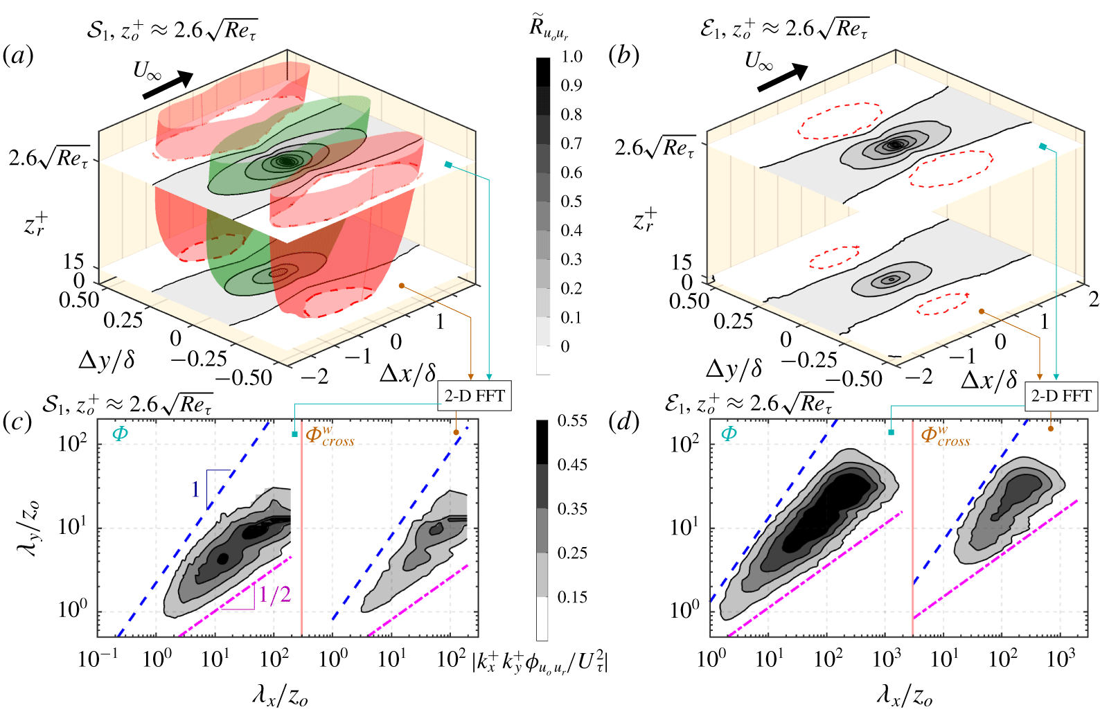
(a) 3-D representation of  $\widetilde{{\mathcal{R}}}_{u_{o}u_{r}}$ for dataset
 ${\mathcal{S}}_{1}$ with
 $z_{o}^{+}\approx 2.6\sqrt{Re_{\unicode[STIX]{x1D70F}}}$ (
 $=120$) as a reference and
 $15\lesssim z_{r}^{+}<150$ to plot isosurfaces for
 $\widetilde{{\mathcal{R}}}_{u_{o}u_{r}}=0.1$ (green) and
 $-0.04$ (red). Wall-parallel planes at
 $z_{r}^{+}\approx 2.6\sqrt{Re_{\unicode[STIX]{x1D70F}}}$ and 15 have positive
 $\widetilde{{\mathcal{R}}}_{u_{o}u_{r}}$ contours as solid lines at levels 0.0 : 0.1 : 1.0 and a dashed red contour for
 $-0.04$. (b) Experimentally (
 ${\mathcal{E}}_{1}$) reconstructed
 $\widetilde{{\mathcal{R}}}_{u_{o}u_{r}}$ at equivalent
 $z_{o}^{+}$ and
 $z_{r}^{+}$ as in (a) and the same contour levels. (c,d)
 $\unicode[STIX]{x1D6F7}$ and
 $\unicode[STIX]{x1D6F7}_{cross}^{w}$ for datasets (c)
 ${\mathcal{S}}_{1}$ and (d)
 ${\mathcal{E}}_{1}$ obtained on computing 2-D FFT of the corresponding 2-D
 $\widetilde{{\mathcal{R}}}_{u_{o}u_{r}}$ plotted in (a) and (b). Contours in (c) and (d) represent energy levels 0.15 : 0.10 : 0.55. Dot-dashed magenta and dashed blue lines represent the square-root and linear relationship, respectively.

While  $\unicode[STIX]{x1D6F7}(z_{o})$ gives the energy distribution of all coexisting eddies at
 $z_{o}$,
 $\unicode[STIX]{x1D6F7}_{cross}^{w}$ (
 $z_{o},z_{r}$) indicates the energy contributed by only those eddies at
 $z_{o}$ that have coherence at the wall (i.e. are ‘wall-attached’). We attempt to explain this difference by first investigating the cross-correlations,
 $\widetilde{{\mathcal{R}}}_{u_{o}u_{r}}$. Figure 2(a) shows the positive and negative isosurfaces of
 $\widetilde{{\mathcal{R}}}_{u_{o}u_{r}}$ considered from a correlation volume,
 $\widetilde{{\mathcal{R}}}_{u_{o}u_{r}}(\unicode[STIX]{x0394}x,\unicode[STIX]{x0394}y,z_{r};z_{o})$, obtained for
 $z_{o}^{+}\approx 2.6\sqrt{Re_{\unicode[STIX]{x1D70F}}}$ and
 $15\lesssim z_{r}^{+}<150$ for dataset
 ${\mathcal{S}}_{1}$. The plot is essentially similar in concept to figure 1 of Sillero et al. (Reference Sillero, Jiménez and Moser2014). Considering a wall-parallel plane at
 $z_{r}=z_{o}$ in this correlation volume gives a 2-D
 $\widetilde{{\mathcal{R}}}_{u_{o}u_{r}}$ map which is analogous to the experimental 2-D correlation obtained via the probe arrangement shown in figure 1(ai) and plotted at
 $z_{r}^{+}\approx 2.6\sqrt{Re_{\unicode[STIX]{x1D70F}}}$ in figure 2(b). Now, by considering a wall-parallel plane at
 $z_{r}^{+}$
 ${\approx}$ 15 in figure 2(a), we get a 2-D map of
 $u$-correlation between the log (
 $z_{o}^{+}\approx 2.6\sqrt{Re_{\unicode[STIX]{x1D70F}}}$) and the near-wall (
 $z_{r}^{+}\approx 15$) region. An experimental analogue of such a correlation is reconstructed with the probe arrangement shown in figure 1(aii) and is plotted in figure 2(b) at
 $z_{r}^{+}\approx 15$. A qualitative comparison between the respective
 $\widetilde{{\mathcal{R}}}_{u_{o}u_{r}}$ maps from the two datasets shows good consistency: (i) The length and width of a particular
 $\widetilde{{\mathcal{R}}}_{u_{o}u_{r}}$ contour level reduces as
 $z_{r}^{+}$ is varied from
 $z_{o}^{+}$ towards the wall. This is consistent with the observations of del Alamo et al. (Reference del Alamo, Jiménez, Zandonade and Moser2004), who attributed this decrease to the absence of the contributions from wall-detached eddies as
 $z_{r}^{+}\rightarrow 0$. (ii) The positive
 $u$-correlations at the spanwise centre (
 $\unicode[STIX]{x0394}y=0$) are flanked by the negative correlations on either side, which extend all the way from the log-region to the wall. This is representative of the adjacent wall-attached low- and high-momentum zones responsible for the streaky pattern in the TBL (Hutchins & Marusic Reference Hutchins and Marusic2007; Hwang & Sung Reference Hwang and Sung2018).
A 2-D Fourier transform of the respective wall-parallel  $\widetilde{{\mathcal{R}}}_{u_{o}u_{r}}$ planes in figures 2(a,b), following (1.2), gives the corresponding 2-D spectral energy distribution plotted in figures 2(c,d). In each of these plots,
 $\unicode[STIX]{x1D6F7}$ and
 $\unicode[STIX]{x1D6F7}_{cross}^{w}$ as a function of the wavelengths scaled with
 $z_{o}$ are plotted on the left and right, respectively. The energy distribution in
 $\unicode[STIX]{x1D6F7}_{cross}^{w}$ is restricted to large
 $\unicode[STIX]{x1D706}_{x}$ and
 $\unicode[STIX]{x1D706}_{y}$, with negligible energy in the small scales:
 $\unicode[STIX]{x1D706}_{x}\lesssim 14z_{o}$,
 $\unicode[STIX]{x1D706}_{y}\lesssim 2z_{o}$, which is unlike the scenario observed for
 $\unicode[STIX]{x1D6F7}$. This can be explained by
 $z_{o}^{+}\gg z_{r}^{+}$, meaning that only physically large wall-attached eddies would appear in
 $\unicode[STIX]{x1D6F7}_{cross}^{w}(z_{o})$. In the forthcoming subsection, we compare
 $\unicode[STIX]{x1D6F7}(z_{o})$ and
 $\unicode[STIX]{x1D6F7}_{cross}(z_{o},z_{r})$ obtained from the two datasets.
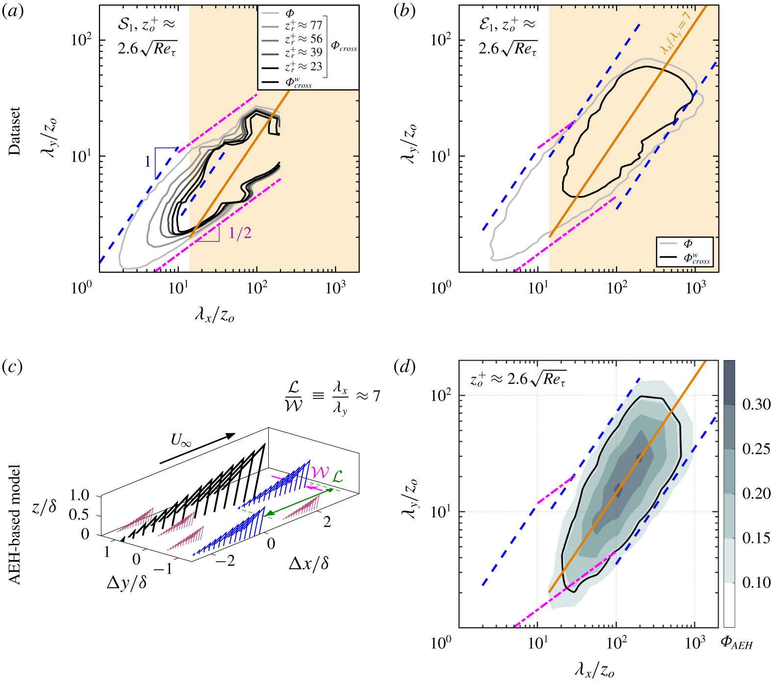
(a,b) 2-D energy spectra for  $z_{o}^{+}\approx 2.6\sqrt{Re_{\unicode[STIX]{x1D70F}}}$ and various
 $z_{r}^{+}$ at a constant energy level of 0.2 for datasets (a)
 ${\mathcal{S}}_{1}$ and (b)
 ${\mathcal{E}}_{1}$. Light yellow background indicates
 $\unicode[STIX]{x1D706}_{x}/z_{o}>14$. (c) Schematic of the AEH-based model considered, shown here having three distinct hierarchies of self-similar wall-attached eddies, with the largest eddy (in black) of the order of
 $\unicode[STIX]{x1D6FF}$.
 ${\mathcal{L}}$ and
 ${\mathcal{W}}$ denote the length and width of an eddy hierarchy, respectively. (d) 2-D spectra obtained from the AEH-based model for
 $Re_{\unicode[STIX]{x1D70F}}\approx 15\,000$ and
 $z_{o}^{+}\approx 2.6\sqrt{Re_{\unicode[STIX]{x1D70F}}}$. Solid black contour is qualitatively equivalent (
 ${\sim}0.5(\unicode[STIX]{x1D6F7}_{AEH})_{max}$) to the one in (b). In (a,b,d), dot-dashed magenta, dashed blue and solid yellow lines denote
 $\unicode[STIX]{x1D706}_{y}/z_{o}\sim (\unicode[STIX]{x1D706}_{x}/z_{o})^{1/2}$,
 $\unicode[STIX]{x1D706}_{y}/z_{o}\sim \unicode[STIX]{x1D706}_{x}/z_{o}$ and
 $\unicode[STIX]{x1D706}_{x}/\unicode[STIX]{x1D706}_{y}=7$ relationships, respectively.

3.2 Low- versus high-$Re_{\unicode[STIX]{x1D70F}}$ 2-D spectra

Figure 3(a) shows the energy spectra for  $z_{o}^{+}\approx 2.6\sqrt{Re_{\unicode[STIX]{x1D70F}}}$ and various
 $z_{r}^{+}$ at a constant energy level of 0.2 for the low-
 $Re_{\unicode[STIX]{x1D70F}}$ dataset (
 ${\mathcal{S}}_{1}$). Also shown are dot-dashed magenta and dashed blue lines which represent the square-root and linear relationship, respectively. As discussed by del Alamo et al. (Reference del Alamo, Jiménez, Zandonade and Moser2004) and Chandran et al. (Reference Chandran, Baidya, Monty and Marusic2017), constant-energy contours of
 $\unicode[STIX]{x1D6F7}$ follow a linear relationship (
 $\unicode[STIX]{x1D706}_{y}\sim \unicode[STIX]{x1D706}_{x}$) only in the small-scale region:
 $\unicode[STIX]{x1D706}_{x}/z_{o},\unicode[STIX]{x1D706}_{y}/z_{o}<10$. It changes to a square-root relationship (
 $\unicode[STIX]{x1D706}_{y}\sim {\unicode[STIX]{x1D706}_{x}}^{1/2}$) at larger scales, suggesting a failure of self-similarity at low
 $Re_{\unicode[STIX]{x1D70F}}$. On the other hand, if we consider the cross-spectra, the constant-energy contours in the same large-scale range depart from the square-root towards a linear behaviour as
 $z_{r}$ approaches the wall (i.e. for
 $\unicode[STIX]{x1D6F7}_{cross}^{w}$). This suggests that the energetic wall-attached eddies are predominantly self-similar. Further, this self-similar trend is obscured in
 $\unicode[STIX]{x1D6F7}$ by energy contributions from the wall-detached eddies. It is obvious, however, that a larger scale separation (i.e. higher
 $Re_{\unicode[STIX]{x1D70F}}$) would better highlight the changing trend with
 $z_{r}$.
Figure 3(b) shows constant-energy contours ( ${\sim}0.2$) of
 $\unicode[STIX]{x1D6F7}$ and
 $\unicode[STIX]{x1D6F7}_{cross}^{w}$ from the high-
 $Re_{\unicode[STIX]{x1D70F}}$ dataset,
 ${\mathcal{E}}_{1}$, with the range of scales increased by almost a decade. Consistent with the observations made by Chandran et al. (Reference Chandran, Baidya, Monty and Marusic2017), for the 2-D spectrum
 $\unicode[STIX]{x1D6F7}$, the square-root relationship for the intermediate range of scales deviates towards a relatively higher power law at
 $\unicode[STIX]{x1D706}_{x}\sim 100z_{o}$ and
 $\unicode[STIX]{x1D706}_{y}\sim 15z_{o}$, with the large scales having an average aspect ratio of
 $\unicode[STIX]{x1D706}_{x}/\unicode[STIX]{x1D706}_{y}\approx 7$ (indicated by a dark yellow line). According to Chandran et al. (Reference Chandran, Baidya, Monty and Marusic2017), this ratio is significant since the large-scale energetic structures in a ZPG TBL become self-similar only after evolving into such large aspect ratios. As opposed to
 $\unicode[STIX]{x1D6F7}$, the energetic ridge of
 $\unicode[STIX]{x1D6F7}_{cross}^{w}$ is seen to follow
 $\unicode[STIX]{x1D706}_{x}/\unicode[STIX]{x1D706}_{y}=7$ along its entire stretch with negligible energy distribution in the scale range where
 $\unicode[STIX]{x1D6F7}$ contours vary as
 $\unicode[STIX]{x1D706}_{y}/z_{o}\sim (\unicode[STIX]{x1D706}_{x}/z_{o})^{1/2}$. The high-
 $Re_{\unicode[STIX]{x1D70F}}$
 $\unicode[STIX]{x1D6F7}_{cross}^{w}$ hence provides convincing evidence of the self-similarity of wall-attached eddies. The fact that the energetic structures contributing to
 $\unicode[STIX]{x1D6F7}_{cross}^{w}$ are restricted to
 $\unicode[STIX]{x1D706}_{x}>14z_{o}$ (highlighted by yellow background), which is consistent with the streamwise inner-scaling limit of self-similar wall-attached structures (Baars et al. Reference Baars, Hutchins and Marusic2017), further adds credence to our claim. Given that
 $\unicode[STIX]{x1D6F7}_{cross}^{w}$ contours follow
 $\unicode[STIX]{x1D706}_{x}/\unicode[STIX]{x1D706}_{y}\approx 7$ and
 $\unicode[STIX]{x1D706}_{x}>14z_{o}$, present analysis suggests
 $\unicode[STIX]{x1D706}_{y}>2z_{o}$ as the plausible spanwise inner-scaling limit for the wall-attached self-similar eddies.
The experimentally obtained  $\unicode[STIX]{x1D6F7}_{cross}^{w}$ is qualitatively similar to the 2-D energy spectrum (
 $\unicode[STIX]{x1D6F7}_{AEH}$) computed from a flow field consisting purely of self-similar wall-attached eddies, as shown in figure 3(d).
 $\unicode[STIX]{x1D6F7}_{AEH}$, here, is obtained using an AEH-based model (Perry et al. Reference Perry, Henbest and Chong1986; Baidya et al. Reference Baidya, Philip, Hutchins, Monty and Marusic2017; Chandran et al. Reference Chandran, Baidya, Monty and Marusic2017) where the log-region is statistically represented by continuous hierarchies of representative eddies whose geometric sizes scale with
 $z_{o}$ and whose probability density varies inversely with
 $z_{o}$. The idea is illustrated in figure 3(c), where, for clarity, the model is depicted in a discretized form with three distinct hierarchies. Heights of the smallest and largest eddies are taken as 100 viscous units and
 $\unicode[STIX]{x1D6FF}$, respectively, with each eddy inclined with respect to
 $x$ at
 $45^{\circ }$ (Deshpande et al. Reference Deshpande, Monty and Marusic2019). The aspect ratio of the eddy hierarchy is roughly equivalent to the ratio of the large scales observed in the high-
 $Re_{\unicode[STIX]{x1D70F}}$ results. Figure 3(d) plots the 2-D spectrum generated from this model at conditions similar to dataset
 ${\mathcal{E}}_{1}$:
 $Re_{\unicode[STIX]{x1D70F}}\approx 15\,000$ and
 $z_{o}^{+}=2.6\sqrt{Re_{\unicode[STIX]{x1D70F}}}$. It can be noted that the high-
 $Re_{\unicode[STIX]{x1D70F}}$
 $\unicode[STIX]{x1D6F7}_{cross}^{w}$ contours show a good correspondence with
 $\unicode[STIX]{x1D6F7}_{AEH}$ contours, which follow the
 $\unicode[STIX]{x1D706}_{y}/z_{o}\sim \unicode[STIX]{x1D706}_{x}/z_{o}$ relation given the imposition of self-similarity.
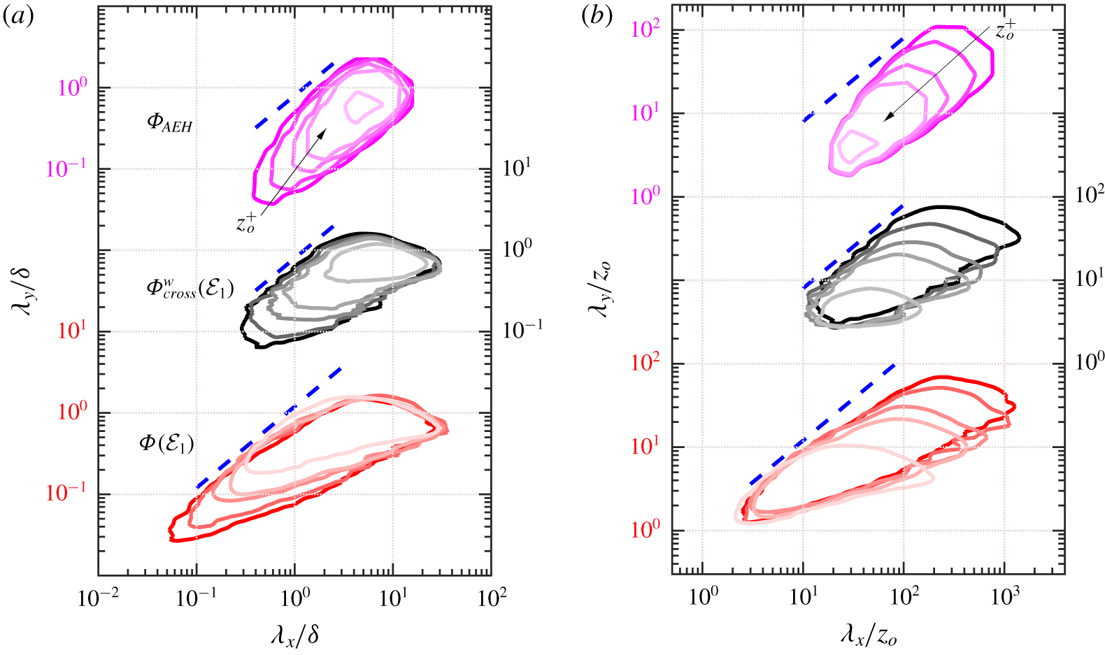
(a,b) Contours at a constant energy level of  $0.35(\unicode[STIX]{x1D6F7}_{AEH})_{max}$,
 $0.35(\unicode[STIX]{x1D6F7}_{cross}^{w})_{max}$ (dataset
 ${\mathcal{E}}_{1}$) and
 $0.35(\unicode[STIX]{x1D6F7})_{max}$ (dataset
 ${\mathcal{E}}_{1}$) for
 $z_{o}^{+}$ across the log-region (table 1) plotted as a function of wavelengths scaled with (a)
 $\unicode[STIX]{x1D6FF}$ and (b)
 $z_{o}$. Dark to light shade indicates an increase in
 $z_{o}^{+}$. For each of the respective spectra, a maximum value at
 $z_{o}^{+}\approx 2.6\sqrt{Re_{\unicode[STIX]{x1D70F}}}$ was considered as a reference to normalize the energy spectra at all
 $z_{o}^{+}$. Dashed blue lines represent the linear power-law relationship for respective spectra.

We extend this qualitative comparison between  $\unicode[STIX]{x1D6F7}_{cross}^{w}$ and
 $\unicode[STIX]{x1D6F7}_{AEH}$ to investigate their scaling in the context of the spectral-overlap arguments of Perry et al. (Reference Perry, Henbest and Chong1986). According to their arguments, the energy contribution from self-similar eddies would follow both outer-flow scaling (
 $\unicode[STIX]{x1D6FF}$-scaling) and inner-flow scaling (
 $z_{o}$-scaling) in the wavelength range corresponding to
 ${\sim}O(\unicode[STIX]{x1D6FF})$ and
 $O(z_{o})$, respectively. These scaling arguments are illustrated in figure 4 using
 $\unicode[STIX]{x1D6F7}_{cross}^{w}$ and
 $\unicode[STIX]{x1D6F7}_{AEH}$, for all
 $z_{o}^{+}$ corresponding to
 ${\mathcal{E}}_{1}$ (table 1), wherein the wavelengths are scaled with
 $\unicode[STIX]{x1D6FF}$ (figure 4a) and
 $z_{o}$ (figure 4b) respectively.
 $\unicode[STIX]{x1D6F7}(z_{o})$ is also plotted at the same
 $z_{o}^{+}$ to demonstrate the effectiveness of the wall filter. A noteworthy observation from figure 4 is that both
 $\unicode[STIX]{x1D6F7}_{AEH}$ and
 $\unicode[STIX]{x1D6F7}_{cross}^{w}$ contours exhibit the
 $\unicode[STIX]{x1D6FF}$- and
 $z_{o}$-scalings in a similar wavelength range. This is suggested by the overlapping constant-energy contours for the respective spectra at various
 $z_{o}^{+}$. Further, these contours indicate an energy distribution predominantly in the large-eddy region (Chandran et al. Reference Chandran, Baidya, Monty and Marusic2017), where they closely follow the
 $\unicode[STIX]{x1D706}_{y}/z_{o}\sim \unicode[STIX]{x1D706}_{x}/z_{o}$ relationship. This supports the claim that
 $\unicode[STIX]{x1D6F7}_{cross}^{w}$ predominantly consists of the contribution from the self-similar eddies that comply with Townsend’s AEH. This contribution can be seen to decrease for both
 $\unicode[STIX]{x1D6F7}_{AEH}$ and
 $\unicode[STIX]{x1D6F7}_{cross}^{w}$ as distance from the wall increases, with energy at
 $z_{o}^{+}\approx 0.15\unicode[STIX]{x1D6FF}^{+}$ (light shaded contours) effectively representing the contribution only from the tall wall-attached structures extending beyond the log-region. In the case of
 $\unicode[STIX]{x1D6F7}$, on the other hand, the
 $z_{o}$-scaling is also observed in the small scales, which are predominantly wall-detached and hence do not show up in
 $\unicode[STIX]{x1D6F7}_{cross}^{w}$. However, the wavelength range exhibiting
 $\unicode[STIX]{x1D6FF}$-scaling is similar to that observed for
 $\unicode[STIX]{x1D6F7}_{cross}^{w}$.
3.3 Is a wall filter sufficient to extract purely self-similar structures?
Referring to the discussion in § 1, on the studies by Baars et al. (Reference Baars, Hutchins and Marusic2017) and Hwang & Sung (Reference Hwang and Sung2018),  $\unicode[STIX]{x1D6F7}_{cross}^{w}(z_{o})$ may be interpreted as the wall-filtered subset of
 $\unicode[STIX]{x1D6F7}(z_{o})$. Recent studies by Baars & Marusic (Reference Baars and Marusic2020) and Yoon et al. (Reference Yoon, Hwang, Yang and Sung2020) show that not all wall-attached structures exhibit self-similarity, and some of them may be geometrically non-self-similar. Given the qualitative resemblance between
 $\unicode[STIX]{x1D6F7}_{cross}^{w}$ and
 $\unicode[STIX]{x1D6F7}_{AEH}$ (§ 3.2), it is worth investigating here if the energy contributions isolated via the wall filter correspond purely to self-similar structures, or there are also contributions from the non-self-similar structures. To this end, we probe the energetic ridges (Chandran et al. Reference Chandran, Baidya, Monty and Marusic2017) of
 $\unicode[STIX]{x1D6F7}$ and
 $\unicode[STIX]{x1D6F7}_{cross}^{w}$, as self-similarity requires the slope (
 $m$) of the ridge to be equal to one (
 $\unicode[STIX]{x1D706}_{y}\sim \unicode[STIX]{x1D706}_{x}$). Here, the energetic ridge of the spectrum is computed by identifying the spanwise wavelength,
 $\unicode[STIX]{x1D706}_{y}$, corresponding to the maximum value of the spectrum at each streamwise wavelength,
 $\unicode[STIX]{x1D706}_{x}$. Additionally, Chandran et al. (Reference Chandran, Baidya, Monty and Marusic2017) has shown that the slope of the ridge translates as the ratio of the plateaus in the 1-D streamwise
 $u$-spectrum to those in the 1-D spanwise
 $u$-spectrum. Here, the 1-D streamwise and spanwise spectra are obtained by integrating the 2-D spectrum along
 $\unicode[STIX]{x1D706}_{y}$ and
 $\unicode[STIX]{x1D706}_{x}$, respectively.
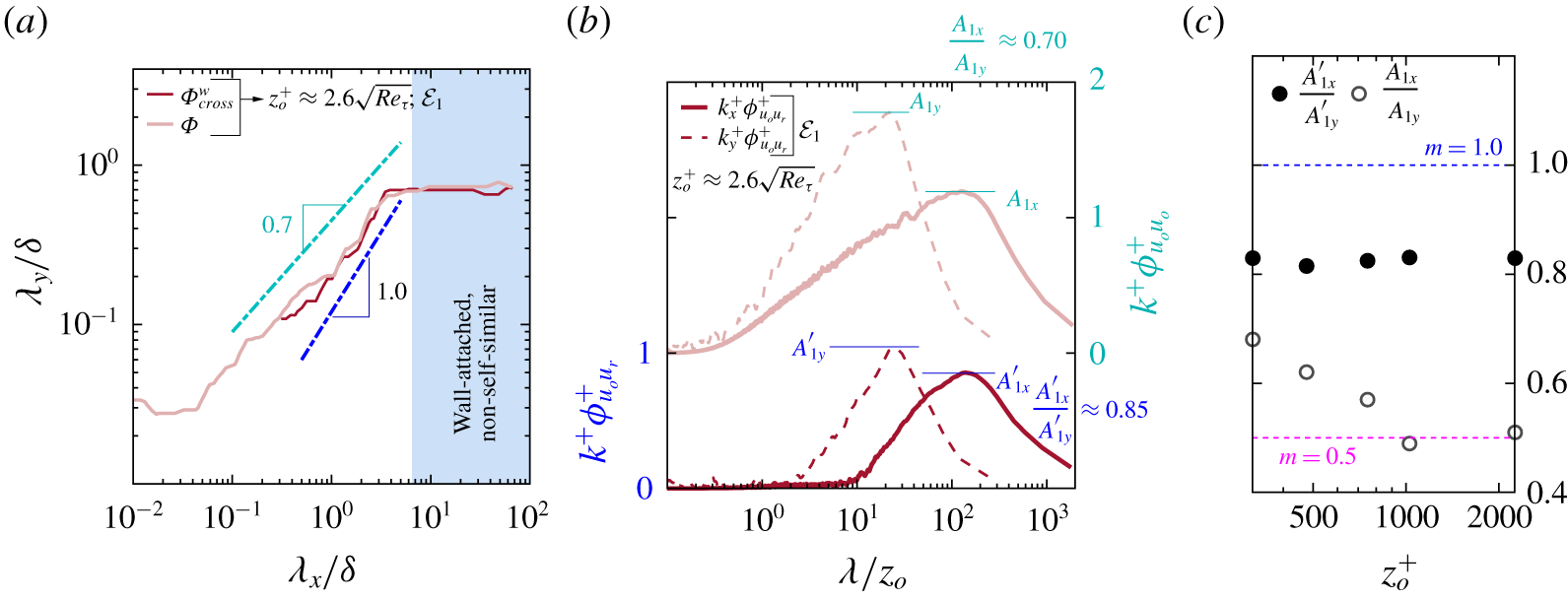
(a) Energetic ridges of  $\unicode[STIX]{x1D6F7}$ (light shaded) and
 $\unicode[STIX]{x1D6F7}_{cross}^{w}$ (dark shaded) for
 $z_{o}^{+}\approx 2.6\sqrt{Re_{\unicode[STIX]{x1D70F}}}$ from dataset
 ${\mathcal{E}}_{1}$, plotted against
 $\unicode[STIX]{x1D6FF}$-scaled wavelengths alongside the power laws indicated by dot-dashed lines. (b) 1-D spanwise and streamwise (cross-)spectrum obtained on integrating the corresponding
 $\unicode[STIX]{x1D6F7}$ (
 $\unicode[STIX]{x1D6F7}_{cross}^{w}$) for
 $z_{o}^{+}\approx 2.6\sqrt{Re_{\unicode[STIX]{x1D70F}}}$ from
 ${\mathcal{E}}_{1}$. Also highlighted are the peaks of the 1-D spectrum (
 $A_{1x},A_{1y}$) and cross-spectrum (
 $A_{1x}^{\prime },A_{1y}^{\prime }$). (c)
 $A_{1x}/A_{1y}$ and
 $A_{1x}^{\prime }/A_{1y}^{\prime }$ estimated at all
 $z_{o}^{+}$ corresponding to
 ${\mathcal{E}}_{1}$ (table 1) by following the methodology shown in (b).

Figure 5(a) shows the energetic ridges of  $\unicode[STIX]{x1D6F7}$ and
 $\unicode[STIX]{x1D6F7}_{cross}^{w}$ for
 $z_{o}^{+}\approx 2.6\sqrt{Re_{\unicode[STIX]{x1D70F}}}$, while figure 5(b) shows the respective 1-D spectra.
 $A_{1x}$ and
 $A_{1y}$ denote the peaks in the 1-D streamwise and spanwise spectra, respectively, while
 $A_{1x}^{\prime }$ and
 $A_{1y}^{\prime }$ refer to the peaks in the 1-D streamwise and spanwise cross-spectra, respectively. These peaks conform to the scale range where the 1-D spectrum is expected to plateau at very high
 $Re_{\unicode[STIX]{x1D70F}}$ (Chandran et al. Reference Chandran, Baidya, Monty and Marusic2017), and is hence used as a reference over here for analysis purposes. Direct computation of
 $m$, from the ratio of the 1-D spectra peaks, shows a difference from 0.7 (for
 $\unicode[STIX]{x1D6F7}$) to 0.85 for
 $\unicode[STIX]{x1D6F7}_{cross}^{w}$, suggesting a relatively greater contribution from self-similar structures to
 $\unicode[STIX]{x1D6F7}_{cross}^{w}$. A change in slope is also evident from the comparison between the energetic ridges of
 $\unicode[STIX]{x1D6F7}$ and
 $\unicode[STIX]{x1D6F7}_{cross}^{w}$. Figure 5(c) plots
 $m$, directly computed from
 $A_{1x}/A_{1y}$ and
 $A_{1x}^{\prime }/A_{1y}^{\prime }$ for
 $\unicode[STIX]{x1D6F7}$ and
 $\unicode[STIX]{x1D6F7}_{cross}^{w}$ respectively, at all
 $z_{o}^{+}$ corresponding to
 ${\mathcal{E}}_{1}$ (table 1). Here,
 $A_{1x}/A_{1y}$ can be seen decreasing with an increase in
 $z_{o}^{+}$. This is consistent with the observations of Chandran et al. (Reference Chandran, Baidya, Monty and Marusic2017), who linked this trend with the AEH prediction on the decrease in self-similar eddy population with distance from the wall (Townsend Reference Townsend1976). Interestingly,
 $A_{1x}^{\prime }/A_{1y}^{\prime }$ on the other hand remains approximately constant (
 ${\approx}$0.85) at all
 $z_{o}^{+}$. This suggests that the variation of
 $A_{1x}/A_{1y}$ with
 $z_{o}^{+}$ is most likely dictated by the contributions from the wall-detached eddies, which are predominantly small, but can be either self-similar or non-self-similar (Marusic & Monty Reference Marusic and Monty2019; Yoon et al. Reference Yoon, Hwang, Yang and Sung2020).
The increment in  $m$ towards 1.0, when comparing
 $\unicode[STIX]{x1D6F7}$ and
 $\unicode[STIX]{x1D6F7}_{cross}^{w}$, confirms that the wall filter does indeed filter out energy contributions from the non-self-similar structures which are wall-detached. However, the fact that
 $m\approx 0.85$ and not 1.0 suggests that
 $\unicode[STIX]{x1D6F7}_{cross}^{w}$ still consists of contributions from wall-attached non-self-similar structures. This can be better understood on investigating the ridge for
 $\unicode[STIX]{x1D6F7}$ and
 $\unicode[STIX]{x1D6F7}_{cross}^{w}$ (figure 5a) in the scale range:
 $\unicode[STIX]{x1D706}_{x}\gtrsim 7\unicode[STIX]{x1D6FF}$,
 $\unicode[STIX]{x1D706}_{y}\sim \unicode[STIX]{x1D6FF}$, where it appears to plateau at a constant
 $\unicode[STIX]{x1D706}_{y}$ and grows only in
 $\unicode[STIX]{x1D706}_{x}$ for both the spectra. The energetic ridge in this scale range is representative of the energy contribution from the
 $\unicode[STIX]{x1D6FF}$-scaled superstructures (Hutchins & Marusic Reference Hutchins and Marusic2007; Chandran Reference Chandran2019), which are known to have
 $(\unicode[STIX]{x1D706}_{x})_{max}$ up to
 $20\unicode[STIX]{x1D6FF}$ but spanwise width restricted to
 $\unicode[STIX]{x1D706}_{y}\sim \unicode[STIX]{x1D6FF}$. The overlap suggests that
 $\unicode[STIX]{x1D6F7}_{cross}^{w}$, like
 $\unicode[STIX]{x1D6F7}$, also consists of energy contributions from the superstructures which, although wall-attached, cannot be categorized as self-similar structures. The presence of these
 $\unicode[STIX]{x1D6FF}$-scaled non-self-similar wall-attached structures has been noted previously by Baars et al. (Reference Baars, Hutchins and Marusic2017) as well as very recently by Yoon et al. (Reference Yoon, Hwang, Yang and Sung2020), who also described these structures to be tall and reminiscent of the superstructures. The
 $\unicode[STIX]{x1D6F7}_{cross}^{w}$ contour for
 $z_{o}^{+}\approx 0.15\unicode[STIX]{x1D6FF}^{+}$ (figure 4a), which is centred at
 $\unicode[STIX]{x1D706}_{x}\sim 7\unicode[STIX]{x1D6FF}$ and
 $\unicode[STIX]{x1D706}_{y}\sim \unicode[STIX]{x1D6FF}$, can be considered representative of the energy contributions from these tall non-self-similar structures. The present analysis thus suggests that this contribution would have to be ‘filtered’ out from the wall-attached energy (at lower
 $z_{o}^{+}$) to obtain the 2-D spectral distribution purely from the self-similar eddies. Our conclusion aligns with the recent work of Baars & Marusic (Reference Baars and Marusic2020), who in addition to a wall filter, also proposed a log-filter in order to isolate the energy contributions from the wall-attached self-similar eddies to the 1-D streamwise spectra. Construction of a robust log-filter, however, is challenging since it requires measurements to be conducted in a physically thick boundary layer and/or at even higher
 $Re_{\unicode[STIX]{x1D70F}}$ than reported in the present study (Baars & Marusic Reference Baars and Marusic2020).
4 Concluding remarks
The present study investigates the 2-D cross-spectrum of  $u$ in a ZPG TBL for
 $Re_{\unicode[STIX]{x1D70F}}$ spanning
 $O(10^{3})$–
 $O(10^{4})$. Special emphasis is laid on the cross-spectrum (
 $\unicode[STIX]{x1D6F7}_{cross}^{w}$) representing coherence between a log (
 $z_{o}$) and a near-wall reference, which depicts the energy distribution across a range of wall-attached eddies existing at
 $z_{o}$, and hence is a subset of the full 2-D spectrum
 $\unicode[STIX]{x1D6F7}(z_{o})$. Removal of the energy contributions from wall-detached eddies results in
 $\unicode[STIX]{x1D6F7}_{cross}^{w}$, at high
 $Re_{\unicode[STIX]{x1D70F}}$, having negligible energy contribution in the scale range where otherwise a
 $\unicode[STIX]{x1D706}_{y}/z_{o}\sim (\unicode[STIX]{x1D706}_{x}/z_{o})^{1/2}$ behaviour is noted for
 $\unicode[STIX]{x1D6F7}$. Further, the energetic large scales contributing to
 $\unicode[STIX]{x1D6F7}_{cross}^{w}$ follow a
 $\unicode[STIX]{x1D706}_{y}/z_{o}\sim \unicode[STIX]{x1D706}_{x}/z_{o}$ power law more closely than seen for
 $\unicode[STIX]{x1D6F7}$. This supports the hypothesis on the obscured view of the self-similar trend for
 $\unicode[STIX]{x1D6F7}$, at finite
 $Re_{\unicode[STIX]{x1D70F}}$, being a result of limited scale separation between various eddies following dissimilar scalings. Further,
 $\unicode[STIX]{x1D6F7}_{cross}^{w}$ closely resembles the qualitative 2-D spectrum obtained from an AEH-based model (
 $\unicode[STIX]{x1D6F7}_{AEH}$), in terms of a scale-specific energy distribution as well as obeyance of the self-similar scaling laws, giving strong evidence of self-similarity ingrained in the TBL. It is shown, however, that
 $\unicode[STIX]{x1D6F7}_{cross}^{w}$ does not represent energy contributions purely from self-similar eddies. At least one more filter is required to remove the contributions from wall-attached non-self-similar structures.
Acknowledgements
The authors wish to acknowledge the Australian Research Council for financial support and thank the authors of Sillero et al. (Reference Sillero, Jiménez and Moser2014) for making their DNS data available. The authors are also grateful to the anonymous reviewers for their helpful comments which improved the quality of the manuscript.
Declaration of interests
The authors report no conflict of interest.