2.1 Problem set-up and governing equations

We consider a cubic cavity of size $L$ filled with air at ambient temperature, heated from below and cooled from above. Top and bottom walls are maintained at uniform temperature $T_{c}$ and $T_{h}$ and the four lateral walls are assumed to be adiabatic. Governing equations under the Boussinesq approximation are

(2.1) $$\begin{eqnarray}\displaystyle & \displaystyle \unicode[STIX]{x1D735}\boldsymbol{\cdot }\boldsymbol{u}=0, & \displaystyle\end{eqnarray}$$

(2.2) $$\begin{eqnarray}\displaystyle & \displaystyle \frac{\unicode[STIX]{x2202}\boldsymbol{u}}{\unicode[STIX]{x2202}t}+\boldsymbol{u}\boldsymbol{\cdot }\unicode[STIX]{x1D735}\boldsymbol{u}=-\unicode[STIX]{x1D735}p+Pr\,\unicode[STIX]{x1D703}\,\boldsymbol{e}_{z}+\frac{Pr}{\sqrt{Ra}}\unicode[STIX]{x1D6FB}^{2}\boldsymbol{u}, & \displaystyle\end{eqnarray}$$

(2.3) $$\begin{eqnarray}\displaystyle & \displaystyle \frac{\unicode[STIX]{x2202}\unicode[STIX]{x1D703}}{\unicode[STIX]{x2202}t}+\boldsymbol{u}\boldsymbol{\cdot }\unicode[STIX]{x1D735}\unicode[STIX]{x1D703}=\frac{1}{\sqrt{Ra}}\unicode[STIX]{x1D6FB}^{2}\unicode[STIX]{x1D703}, & \displaystyle\end{eqnarray}$$

where $\boldsymbol{u}=(u,v,w)$ is the dimensionless velocity vector, $p$ is the dimensionless pressure and $\unicode[STIX]{x1D703}$ is the reduced temperature. A no-slip velocity condition ( $\boldsymbol{u}=0$ ) is prescribed on the six walls of the cavity and thermal boundary conditions are written as follows:

(2.4) $$\begin{eqnarray}\left.\begin{array}{@{}c@{}}\unicode[STIX]{x1D703}=0.5\quad \text{on }z=0,\\ \unicode[STIX]{x1D703}=-0.5\quad \text{on }z=1,\\ \unicode[STIX]{x1D735}\unicode[STIX]{x1D703}\boldsymbol{\cdot }\boldsymbol{n}=0\quad \text{on }x=0,\;x=1,\;y=0,\;y=1,\end{array}\right\}\end{eqnarray}$$

where $x$ , $y$ and $z$ are the dimensionless Cartesian coordinates. The Rayleigh number which controls the flow regime is set to $10^{7}$ and is given by $Ra=g\unicode[STIX]{x1D6FD}_{e}\unicode[STIX]{x0394}TL^{3}/(\unicode[STIX]{x1D708}\unicode[STIX]{x1D705})$ , where $g$ is the gravitational acceleration, $\unicode[STIX]{x1D6FD}_{e}$ is the thermal expansion coefficient, $\unicode[STIX]{x1D708}$ is the kinematic viscosity, $\unicode[STIX]{x1D705}$ is the thermal diffusivity and $\unicode[STIX]{x0394}T=(T_{h}-T_{c})$ is the temperature difference between the hot and cold walls. The Prandtl number is set to 0.707 and is given by $Pr=\unicode[STIX]{x1D708}/\unicode[STIX]{x1D705}$ . Equations are made dimensionless using the length of the cavity $L$ , the reference time $L^{2}/(\unicode[STIX]{x1D705}\sqrt{Ra})$ and the reduced temperature $\unicode[STIX]{x1D703}=(T-T_{0})/\unicode[STIX]{x0394}T$ , $T_{0}$ being the mean temperature between hot and cold walls.

The problem satisfies four independent reflection symmetries $S_{x}$ , $S_{y}$ , $S_{z}$ and $S_{d}$ with respect to the planes $x=0.5$ , $y=0.5$ , $z=0.5$ and $x=y$ (Puigjaner et al. Reference Puigjaner, Herrero, Simo and Giralt2008). These symmetries act on the velocity and temperature fields as follows:

(2.5) $$\begin{eqnarray}\displaystyle & \displaystyle S_{x}:\left.\begin{array}{@{}c@{}}(x,y,z)\rightarrow (1-x,y,z)\\ (u,v,w,\unicode[STIX]{x1D703})\rightarrow (-u,v,w,\unicode[STIX]{x1D703})\end{array}\right\} & \displaystyle\end{eqnarray}$$

(2.6) $$\begin{eqnarray}\displaystyle & \displaystyle S_{y}:\left.\begin{array}{@{}c@{}}(x,y,z)\rightarrow (x,1-y,z)\\ (u,v,w,\unicode[STIX]{x1D703})\rightarrow (u,-v,w,\unicode[STIX]{x1D703})\end{array}\right\} & \displaystyle\end{eqnarray}$$

(2.7) $$\begin{eqnarray}\displaystyle & \displaystyle S_{z}:\left.\begin{array}{@{}c@{}}(x,y,z)\rightarrow (x,y,1-z)\\ (u,v,w,\unicode[STIX]{x1D703})\rightarrow (u,v,-w,-\unicode[STIX]{x1D703})\end{array}\right\} & \displaystyle\end{eqnarray}$$

(2.8) $$\begin{eqnarray}\displaystyle & \displaystyle S_{d}:\left.\begin{array}{@{}c@{}}(x,y,z)\rightarrow (y,x,z)\\ (u,v,w,\unicode[STIX]{x1D703})\rightarrow (v,u,w,\unicode[STIX]{x1D703}).\end{array}\right\} & \displaystyle\end{eqnarray}$$

These four elementary symmetries generate a symmetry group of 16 elements. In the unsteady regime, we expect these symmetries to be satisfied by the time-averaged flow field.

2.2 Numerical methods

Equations (2.1)–(2.3) are solved using a Chebyshev collocation method for the three dimensions of space (Xin & Le Quéré Reference Xin and Le Quéré2002). The pressure–flow coupling is ensured by a projection method, in two steps. First, momentum and energy equations are solved using the previous time step pressure field. Then, a pressure correction term is calculated from a Poisson equation and the predicted velocity is corrected in order to force the velocity divergence free condition. Time integration is performed through a second-order temporal scheme combining a backward differentiation (BDF2) scheme for the linear terms with an Adams–Bashforth extrapolation of convective terms. This algorithm is implemented for parallel computations applying domain decomposition along the vertical $z$ direction (Xin, Chergui & Le Quéré Reference Xin, Chergui, Le Quéré, Tromeur-Dervout, Brenner, Emerson and Erhel2010).

The spatial mesh is made of 81 Chebyshev collocation points in the $x$ and $y$ directions and $4\times 21$ Chebyshev collocation points (4 spatial domains discretized with 21 points) in the $z$ direction. The number of spatial collocation points in the kinetic and thermal boundary layers ( $N_{u,BL}$ and $N_{\unicode[STIX]{x1D703},BL}$ ) is about 10 in the $x$ and $y$ directions and about 6 in the $z$ direction, which is satisfactory regarding the criterion proposed by Shishkina et al. (Reference Shishkina, Stevens, Grossmann and Lohse2010) ( $N_{u,BL}=0.31Ra^{0.15}$ and $N_{\unicode[STIX]{x1D703},BL}=0.35Ra^{0.15}$ for $Pr\simeq 0.7$ ). The thicknesses of the kinetic and thermal boundary layers have been estimated using the correlations provided by the same authors and are, respectively, $\unicode[STIX]{x1D6FF}_{u}/L=0.027$ and $\unicode[STIX]{x1D6FF}_{\unicode[STIX]{x1D703}}/L=0.031$ at $Ra=10^{7}$ .

The dimensionless time step is $2.5\times 10^{-3}$ . Starting from a fluid at $\boldsymbol{u}=\mathbf{0}$ and $\unicode[STIX]{x1D703}=0$ , equations are first integrated over a dimensionless time period of 2000 in order to reach the asymptotic regime and then integrated over a dimensionless time period of 10 000 to conduct the analysis. The time-averaged Nusselt number over this second period is equal to 16.24, which is consistent with the value of 16.57 found by Giannakis et al. (Reference Giannakis, Kolchinskaya, Krasnov and Schumacher2018) for the same Rayleigh number and a nearly identical Prandtl number of 0.7.

2.3 Large-scale flow structures

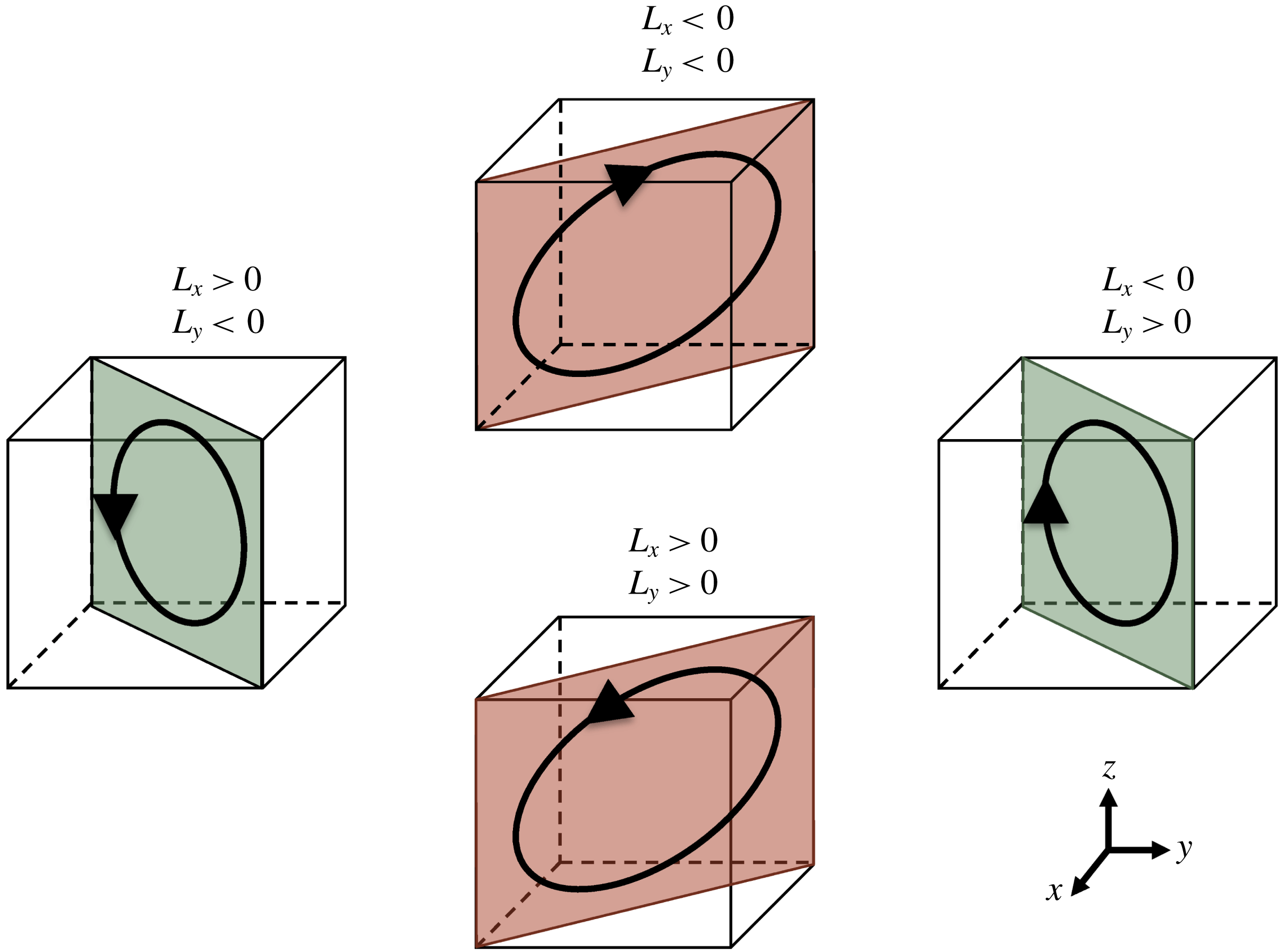
Four quasi-stable flow states are observed in the numerical simulation. The LSC associated with these states consists of a dominant roll in one of the two diagonal planes $x=y$ or $x=1-y$ with a clockwise or anticlockwise motion as shown in figure 1. These four flow states have been reported by other researchers in numerical studies (Foroozani et al. Reference Foroozani, Niemela, Armenio and Sreenivasan2017; Giannakis et al. Reference Giannakis, Kolchinskaya, Krasnov and Schumacher2018; Vasiliev et al. Reference Vasiliev, Frick, Kumar, Stepanov, Sukhanovskii and Verma2019) and experimental studies (Bai et al. Reference Bai, Ji and Brown2016; Vasiliev et al. Reference Vasiliev, Sukhanovskii, Frick, Budnikov, Fomichev, Bolshukhin and Romanov2016).

Figure 1.

Diagram of the four quasi-stable flow states and associated sign of $x$ and $y$ components of the global angular momentum.

The switches between these states can be monitored with the time evolution of the $x$ and $y$ components of the global angular momentum with respect to the centre of the cavity $\boldsymbol{r}_{0}=(0.5;0.5;0.5)$ :

(2.9) $$\begin{eqnarray}\boldsymbol{L}=\int (\boldsymbol{r}-\boldsymbol{r}_{0})\wedge \boldsymbol{u}\,\text{d}\boldsymbol{r},\end{eqnarray}$$

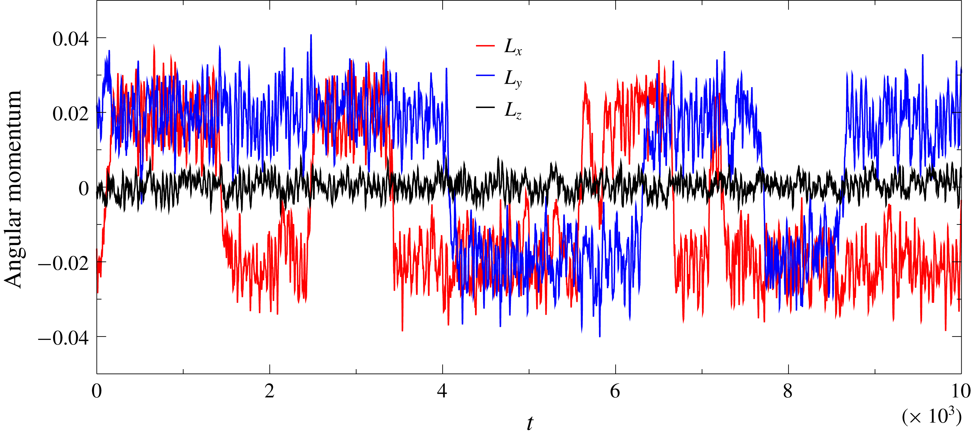
which is plotted in figure 2. Both components $L_{x}$ and $L_{y}$ display quasi-stable periods with moderate oscillations around a mean value of $\pm 0.2$ separated by abrupt aperiodic sign switches. A sign switch of one of the $x$ or $y$ components of the global angular momentum corresponds to a rotation of the LSC of $\unicode[STIX]{x03C0}/2$ from one diagonal plane to another. Such a transition will be referred to as a reorientation of the LSC in the remainder of the paper. Interestingly, a simultaneous sign switch of both $L_{x}$ and $L_{y}$ is never observed in the simulation. This would be equivalent to a flow reversal (as observed in a square Rayleigh–Bénard cell by Podvin & Sergent (Reference Podvin and Sergent2015)) where the direction of rotation of the LSC changes within the same diagonal plane. While the switching mechanism between states is a non-periodic phenomenon, the average time spent in a quasi-stable flow state can be estimated by tracking the sign switches of angular momentum components. About 12 switches were identified in the simulation, which corresponds to a mean period of about 830 units. A more systematic analysis will be carried out in the next section.

Figure 2.

Time evolution of the three components of the angular momentum.

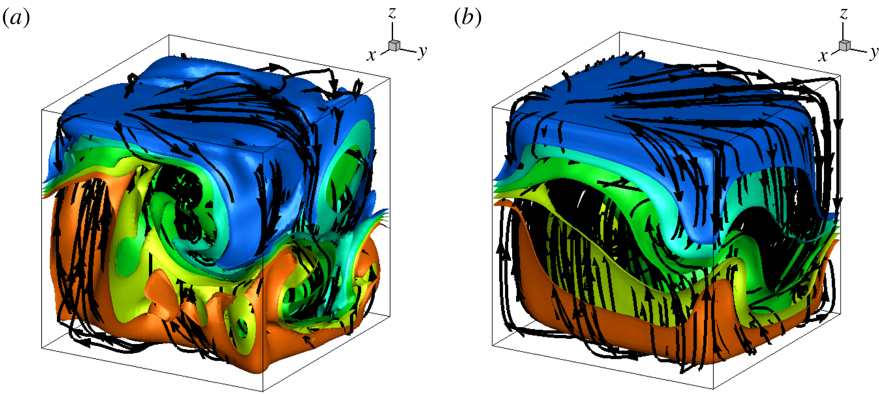
The structure of the flow in one of the quasi-stable states ( $L_{x}<0$ and $L_{y}<0$ ) can be observed in figure 3 where an instantaneous flow field at $t=4610$ and a time-averaged flow field during the period [4500–5500] are shown. A fluid parcel rotates in the diagonal LSC in approximately 50 time units if we take a reference velocity of 0.076, obtained by averaging the absolute value of the vertical velocity in the horizontal mid-plane, and a reference travel path length of 3.85, estimated by an ellipsoid trajectory in the diagonal plane. This estimate agrees well with the dominant oscillatory time scale $T_{c}\sim 45$ identified in the temporal spectrum of the angular momentum. A period of 1000 time units is then sufficient to correctly capture the mean features of the quasi-stable state. The instantaneous and time-averaged flow fields in figure 3 show a LSC lying in the diagonal plane $x=1-y$ . The fluid flows up along the left vertical edge $(x;y)=(1;0)$ and flows down along the right vertical edge $(x;y)=(0;1)$ . This main diagonal roll is slightly tilted and two small counter-rotating rolls are noticeable in the top left corner $(x;y;z)=(1;0;1)$ and in the bottom right corner $(x;y;z)=(0;1;0)$ . Along the isothermal walls, part of the fluid moves away from the main diagonal plane and forms secondary rolls in the opposite corners. These structures spread up to mid-height and get back to the main stream along the two vertical edges of the diagonal plane.

Figure 3.

Instantaneous flow field at $t=4610$ (a) and time-averaged flow field during the period $t\in [4500{-}5500]$ (b). Streamlines and isotherms $\unicode[STIX]{x1D703}=\{0;\pm 0.05;\pm 0.1\}$ .

3.2 The POD spectrum and associated modes

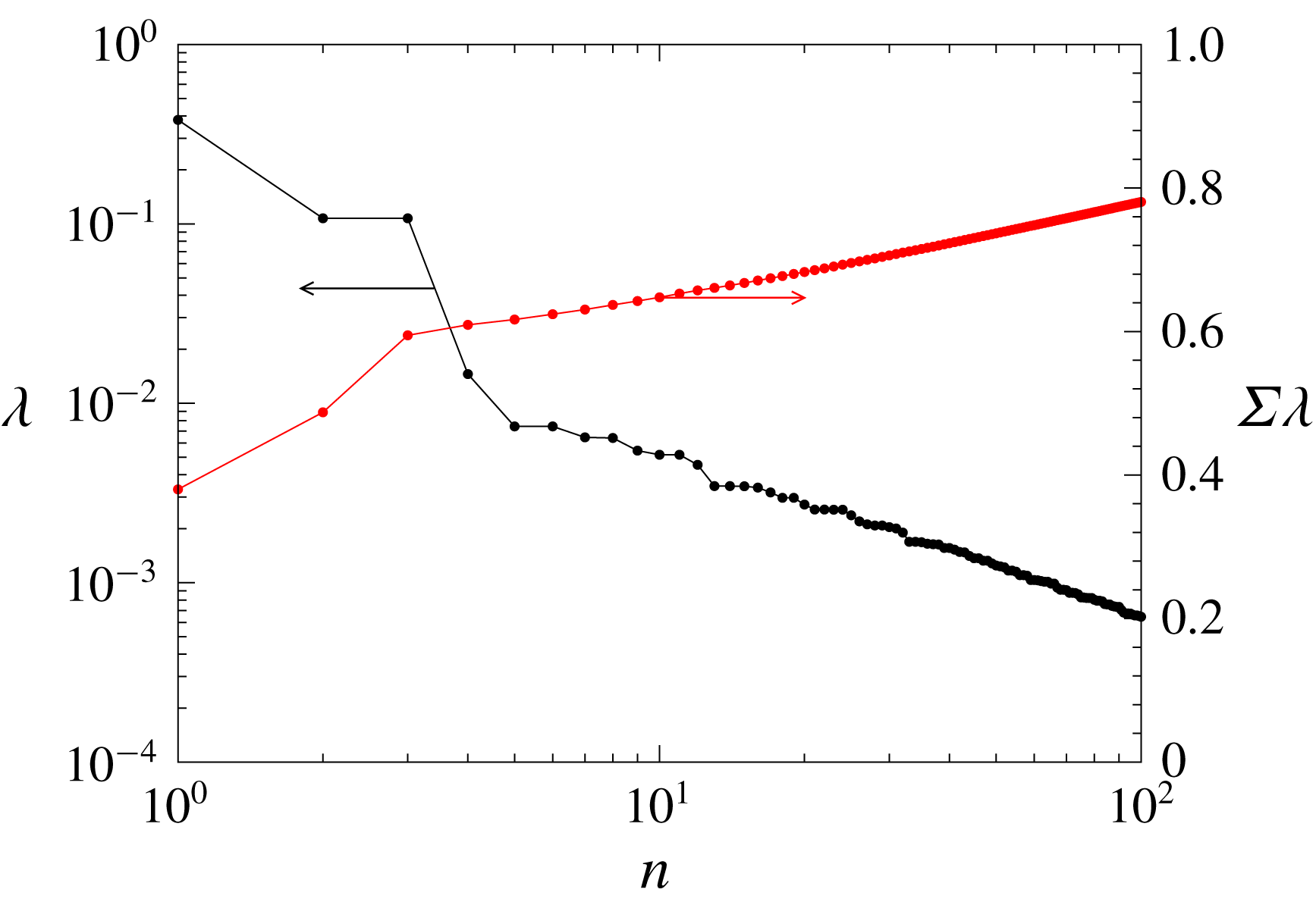
The POD eigenspectrum is shown in figure 4. The decay of the spectrum is rather slow owing to the three dimensions of space and the turbulent nature of the flow. The first three modes contain, however, 60 % of the total energy. An interesting feature of the spectrum is the presence of pairs of degenerated modes with strictly identical eigenvalues, for instance modes 2 and 3, modes 5 and 6 or modes 10 and 11. These pairs of modes result from the equivalence between directions $x$ and $y$ in the horizontal plane and are associated with spatial structures that are the image of each other after a rotation of $\unicode[STIX]{x03C0}/2$ around the $z$ axis. Interestingly, when applying POD to the original (non-symmetrized) snapshot set, we have identified similar pairs of structures, linked by a rotation of $\unicode[STIX]{x03C0}/2$ around the $z$ axis. However one observes a small discrepancy in energy between these modes due to the statistical imbalance between the four quasi-stable flow states. Apart from the first three modes that clearly stand out from the spectrum, it is difficult to decide which modes have to be retained in a reduced decomposition based on an energy criterion. In the following we will restrict the analysis to the first seven modes. This will be justified in § 4 where it will be shown that a seven-mode reduced-order model is able to fairly reproduce the dynamics of the large-scale flow reorientations.

Figure 4.

The POD eigenspectrum normalized such that $\sum _{i}\unicode[STIX]{x1D706}_{i}=1$ (black, left-hand axis) and associated cumulated spectrum (red, right-hand axis).

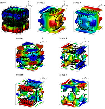
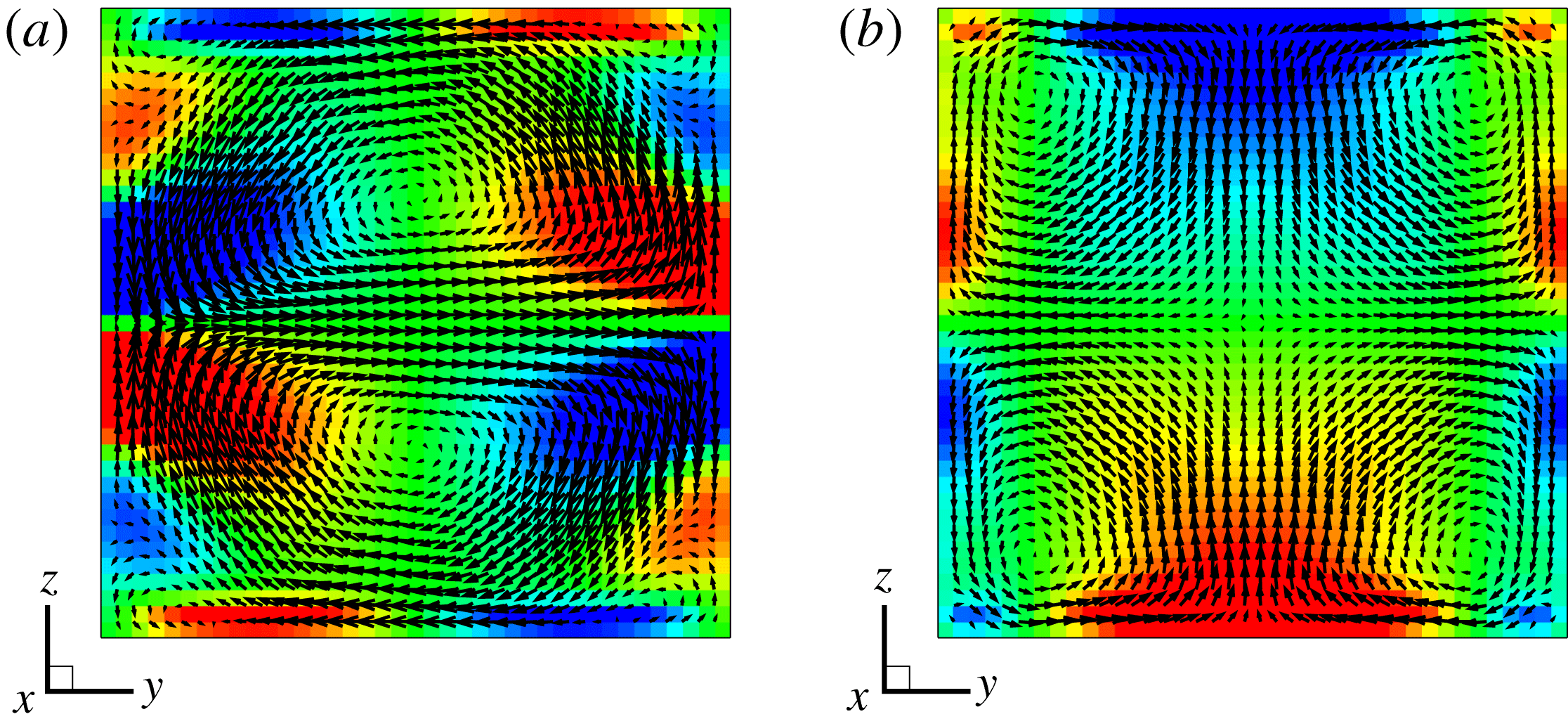
Figure 5 shows the 3-D thermal and flow patterns of the first seven POD modes. Positive iso-surfaces of the $Q$ -criterion ( $Q=-0.5\,\unicode[STIX]{x2202}u_{i}/\unicode[STIX]{x2202}x_{j}\times \unicode[STIX]{x2202}u_{j}/\unicode[STIX]{x2202}x_{i}$ ; Hunt, Wray & Moin (Reference Hunt, Wray and Moin1988)) are used to highlight the rotating zones. The $Q$ -criterion compares strain and vorticity and a positive value means that vorticity is dominant. Temperature and velocity fields of modes 4 and 7 are also displayed in figure 6 in a 2-D vertical plane near the sidewall $x=0$ . 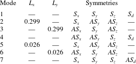In addition, the angular momentum with respect to the $x$ and $y$ directions together with the symmetry properties of the first seven modes are given in table 1.

The first mode corresponds to the mean flow. The velocity field consists of two counter-rotating torus-like structures confined, respectively, to the upper half and the lower half of the cube (the vertical component of the velocity is zero at the horizontal mid-height plane). In the upper (respectively lower) torus, the fluid flows down (up) along the adiabatic walls and turns back to the centre. The temperature field is vertically stratified from the bottom hot wall to the top cold wall. The vertical temperature gradient (heat flux) at the isothermal walls is the highest at the centre and the lowest at the corners. The velocity and temperature fields of this first mode satisfy all the symmetries of the problem and thus the associated global angular momentum is null.

Figure 5.

First seven POD modes. Streamlines and iso-surfaces of $Q$ -criterion ( $Q=5$ for modes 1–3 and $Q=30$ for modes 4–7) coloured by mode temperature. Colourmap for mode temperature ranges from $-0.5$ (blue) to 0.5 (red).

Modes 2 and 3, which have the same eigenvalue, consist of a single roll around the $x$ axis and the $y$ axis, respectively, which correspond to LSC lying in $x$ plane and $y$ plane, respectively. They of course possess a strong global angular momentum with respect to the $x$ axis (mode 2) or the $y$ axis (mode 3) and it can be inferred at this stage that the two modes have to be combined to form the quasi-stable diagonal rolls observed in the simulations. The two modes are identical after a rotation of $\unicode[STIX]{x03C0}/2$ and both break the diagonal symmetry. It can be seen in figure 5 that the temperature field is correlated with the velocity field: the temperature is positive (hot) when the flow is ascending and negative (cold) when the flow is descending. Because these two modes form a pair of degenerated eigenvectors, they are not uniquely defined and they can be replaced in the POD basis by any linear combination of the two original vectors $(\unicode[STIX]{x1D753}_{2},\unicode[STIX]{x1D753}_{3})$ as long as the orthonormality is preserved. Namely, an infinity of eigenvector pairs $(\unicode[STIX]{x1D753}_{2}^{\prime },\unicode[STIX]{x1D753}_{3}^{\prime })$ can be generated, providing that they satisfy $\unicode[STIX]{x1D753}_{2}^{\prime }=\unicode[STIX]{x1D6FC}\unicode[STIX]{x1D753}_{2}+\unicode[STIX]{x1D6FD}\unicode[STIX]{x1D753}_{3}$ and $\unicode[STIX]{x1D753}_{3}^{\prime }=\mp \unicode[STIX]{x1D6FD}\unicode[STIX]{x1D753}_{2}\pm \unicode[STIX]{x1D6FC}\unicode[STIX]{x1D753}_{3}$ , $\unicode[STIX]{x1D6FC}$ and $\unicode[STIX]{x1D6FD}$ being real constants such that $\unicode[STIX]{x1D6FC}^{2}+\unicode[STIX]{x1D6FD}^{2}=1$ . For instance, we could transform the two eigenmodes of figure 5 using $\unicode[STIX]{x1D6FC}=\sqrt{2}/2$ in order to obtain two single-roll modes each lying in one of the two diagonal planes. A diagonal quasi-stable LSC would then be obtained by the activation of one mode and the cancellation of the other. However, we will preserve modes 2 and 3 as pure $x$ -roll and pure $y$ -roll in this study.

Mode 4 is made of eight counter-rotating rolls along the $x$ and $y$ axes with four rolls in the upper half of the cube and four rolls in the lower half of the cube. Like the mean flow, the vertical component of the velocity is zero at the horizontal mid-height plane (see figure 6). The rolls transport fluid from one corner to the other; they are the largest near the adiabatic walls and shrink as they progress towards the mid $z$ axis. Combined with mode 1 (mean flow), mode 4 reinforces the corner flows within one of the two diagonal planes and softens the corner flows within the other orthogonal diagonal plane. We will see later that this mode stabilizes the diagonal flow states. It is interesting to note that the first four POD modes are similar to the four primary Koopman eigenfunctions identified by Giannakis et al. (Reference Giannakis, Kolchinskaya, Krasnov and Schumacher2018). However, the Koopman eigenfunctions presented in their study were not symmetrized. In addition, the Koopman eigenfunctions corresponding to POD modes 2 and 3 were made of a single LSC roll located in the diagonal plane instead of the mid $x$ plane and the mid $y$ plane in our study.

Modes 5 and 6 form another pair of degenerated modes and have been chosen consistently with the pair of modes 2 and 3. Mode 5 is made of two longitudinal co-rotating rolls lying in the mid $x$ plane, one in the upper half of the cell, one in the lower half of the cell. The two rolls are connected by vertical streams along the planes $x=0$ and $x=1$ . The interaction between the horizontal streams in the mid-plane and the vertical streams near the walls gives rise to two small rotating structures that are responsible for a weak global angular momentum along the $x$ axis. Mode 5 possesses the same symmetries as mode 2 suggesting a strong interaction between the two modes. Mode 5 slows down or speeds up mode 2 depending on whether they are combined with the same sign or opposite sign. Mode 6 is the image of mode 5 after a rotation of $\unicode[STIX]{x03C0}/2$ and possesses the same symmetry as mode 3. The relationship between modes 3 and 6 is thus identical to the relationship between modes 2 and 5. Modes 5 and 6 will be referred to as boundary-layer modes in the remainder of the paper.

Mode 7 is similar to mode 4, as it contains eight counter-rotating structures, four confined in the upper half of the cell and four confined in the lower half of the cell. However, the rotation axes of these rolls are aligned along diagonal axes $x=1-y$ and $x=y$ instead of the $x$ axis and the $y$ axis. These rolls bring fluid from the mid $x$ plane to the mid $y$ plane (and vice versa) and we can foresee important coupling with $x$ -plane modal structures (modes 2 and 5) and $y$ -plane modal structures (modes 3 and 6). We can also infer that mode 7 would destabilize a diagonal LSC. Its symmetry properties are opposite to those of mode 4, except for the $S_{z}$ symmetry satisfied by both modes.

To conclude, these 3-D POD modes of the cubic cell can be compared with the 2-D POD modes of the square cell (Podvin & Sergent Reference Podvin and Sergent2017). In that perspective, mode 1 would correspond to the 2-D quadrupolar mode (mean flow). Modes 2 and 3 would correspond to the 2-D LSC mode, the degeneracy coming from the third dimension. Modes 5 and 6 (degenerate) would correspond to the 2-D $L_{\ast }$ mode that connects the core region with the horizontal boundary layers. This last mode has been identified as a precursor for 2-D reversals of the LSC. However, it is worth noting that modes 4 and 7 are pure 3-D modes that have no equivalent structures in the 2-D square case.

Figure 6.

Temperature (colour) and velocity (vectors) fields in the vertical plane $x=0.05$ of POD mode 4 (a) and $x=0.15$ of POD mode 7 (b). Colourmap for temperature ranges from $-0.5$ (blue) to 0.5 (red).

Table 1.

Angular momentum and symmetry properties of the first seven modes. Here $S_{x/y/z/d}$ and $AS_{x/y/z/d}$ denote, respectively, a symmetry and an anti-symmetry with respect to the planes $x=0.5$ , $y=0.5$ , $z=0.5$ and $x=y$ .

3.3 Temporal dynamics

The initial (non-symmetrized) snapshot set has been projected onto the reduced POD basis of seven modes in order to compute the associated DNS POD coefficients at discrete times $t_{i}$ :

(3.7) $$\begin{eqnarray}a_{n}(t_{i})=\int _{\unicode[STIX]{x1D6FA}}\boldsymbol{U}(\boldsymbol{r},t_{i})\boldsymbol{\cdot }\unicode[STIX]{x1D753}_{n}(\boldsymbol{r})\,\text{d}\boldsymbol{r}.\end{eqnarray}$$

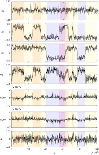
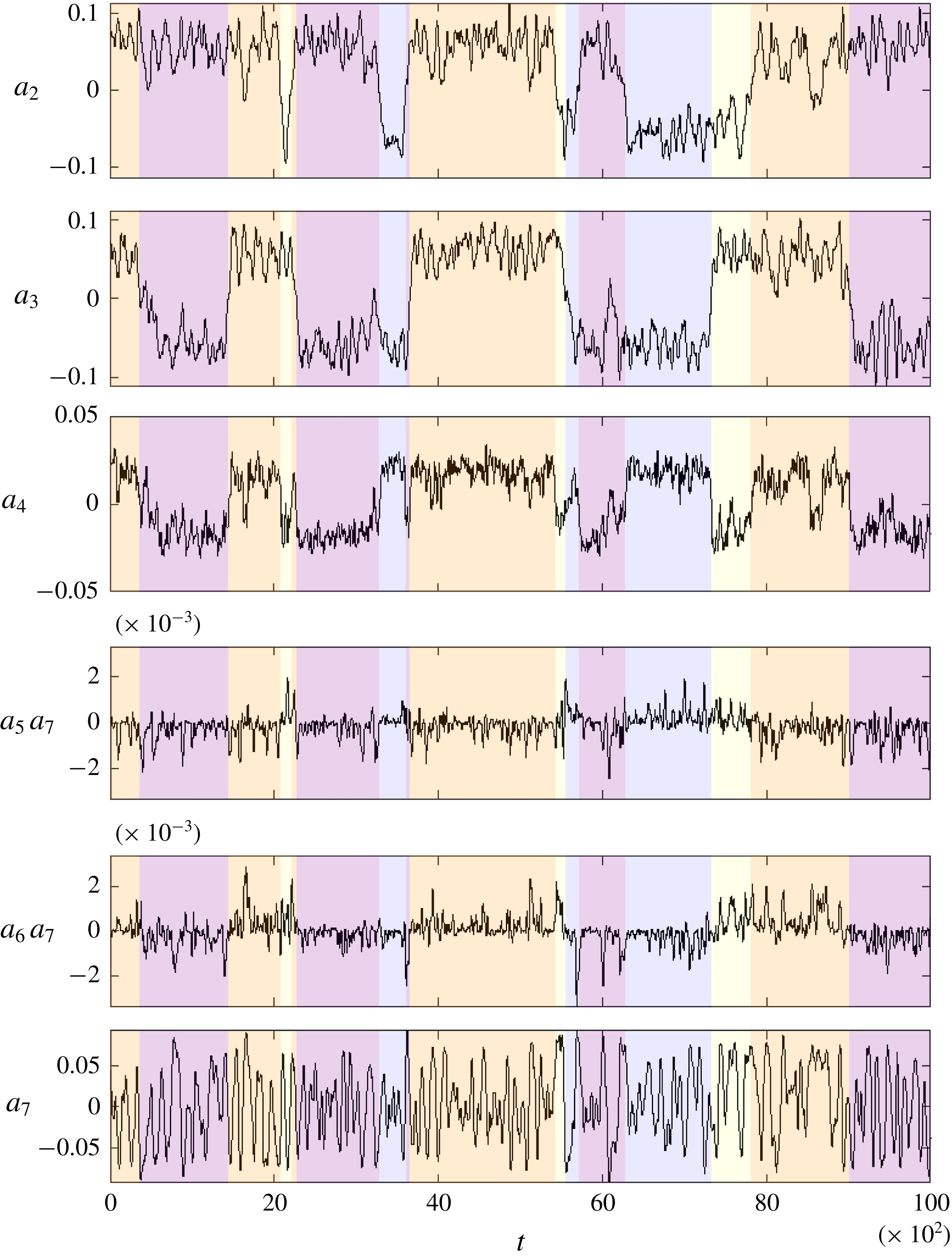
The resulting time evolution of the POD coefficients is shown in figure 7 where dashed lines indicate reorientation events.

As expected, the coefficient associated with the first mode (mean flow) is nearly constant and oscillates around a mean value of $a_{1}^{eq}=\sqrt{\unicode[STIX]{x1D706}_{1}}=0.1271$ . Because modes 2 and 3 are pure $x$ -roll and $y$ -roll, their associated POD coefficients are correlated with the time evolution of the $x$ and $y$ components of the global angular momentum shown in figure 2. Therefore, the coefficients of modes 2 and 3 oscillate around a mean value of $a_{2/3}^{eq}=\pm \sqrt{\unicode[STIX]{x1D706}_{2/3}}=\pm 0.0675$ during the quasi-stable-state period, which confirms that diagonal LSC flows are obtained by superimposing an $x$ -plane LSC (mode 2) and a $y$ -plane LSC (mode 3). We have shown in § 2.3 that reorientations occur when either the $x$ component or the $y$ component of the angular momentum changes sign. From a POD point of view, a reorientation occurs when either the coefficient $a_{2}$ or $a_{3}$ changes sign which corresponds to a reversal (a change of the sense of rotation) of either the $x$ -roll (mode 2) or the $y$ -roll (mode 3). This interpretation agrees with the one proposed by Vasiliev et al. (Reference Vasiliev, Frick, Kumar, Stepanov, Sukhanovskii and Verma2019). We note that a cancellation or cessation of $a_{2}$ (or $a_{3}$ ) may occasionally not result in a reorientation, as can be seen at $t=5800$ in figure 7, where $a_{2}$ drops to values close to zero for a short period before increasing back to the initial amplitude. This physically corresponds to a temporary alignment of the LSC with the sidewalls of the cube followed by a return to the original diagonal state.

It is worth noting that the time evolution of the fourth POD coefficient also follows the reorientation dynamics: $a_{4}$ oscillates around a mean value of $a_{4}^{eq}=\pm \sqrt{\unicode[STIX]{x1D706}_{4}}=\pm 0.0249$ and experiences rapid sign switches at each reorientation. The fourth coefficient is actually strongly correlated with the product of the second and third coefficients ( $a_{4}(t)\propto a_{2}(t)a_{3}(t)$ ). Mode 4 could thus be interpreted as an indicator of the diagonal plane in which the LSC takes place: $a_{4}>0$ means the LSC lies in the plane $x=1-y$ ; $a_{4}<0$ means the LSC lies in the plane $x=y$ .

The time evolution of the fifth to seventh coefficients ( $a_{5}$ and $a_{6}$ not shown) is chaotic with a dominant high frequency around $2\times 10^{-2}$ corresponding to the rotation frequency of the diagonal LSC (see § 2.3) and does not seem to follow any specific pattern during reorientations. However, the time evolution of coefficient products $a_{5}a_{7}$ and $a_{6}a_{7}$ in figure 7 shows an interesting feature: their sign is correlated with, respectively, the opposite of the coefficients of second and third modes. This suggests a strong quadratic interaction between the 2-D rolls (mode 2 or 3), the boundary-layer modes (modes 5 or 6) and the diagonal corner rolls (mode 7). In addition, we will see in § 4 that modes 5 to 7 are necessary in the reduced-order model to produce flow reorientations. The correlation between modes 2 and 5, and between modes 3 and 6, has been further confirmed by applying a moving average over 90 time units to $a_{5}(t)$ and $a_{6}(t)$ , which shows a small equilibrium contribution $a_{5/6}^{eq}$ during quasi-stable states, much lower than the standard deviation $\sqrt{\unicode[STIX]{x1D706}_{5/6}}$ . This equilibrium contribution switches sign at each reversal of the associated planar rolls: $\text{sgn}(a_{5}^{eq})=-\text{sgn}(a_{2}^{eq})$ and $\text{sgn}(a_{6}^{eq})=-\text{sgn}(a_{3}^{eq})$ .

Figure 7.

Time evolution of the DNS POD coefficients. Each quasi-stable state is depicted by a different colour: orange $L_{x}>0,L_{y}>0$ ; yellow $L_{x}<0$ , $L_{y}>0$ ; blue $L_{x}<0,L_{y}<0$ ; purple $L_{x}>0,L_{y}<0$ .

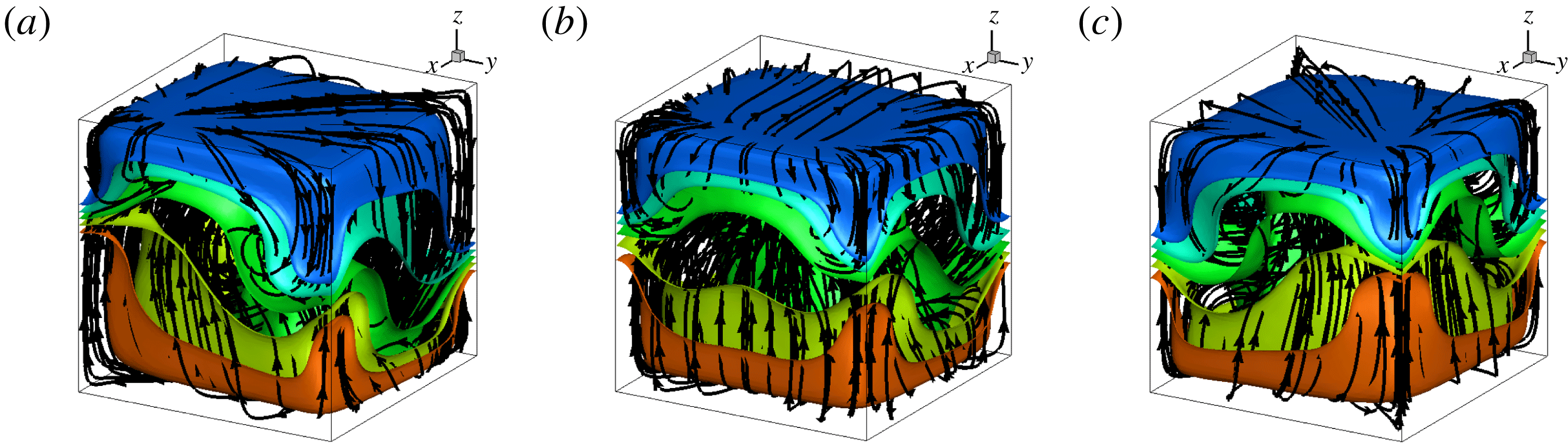
The analysis of the time evolution of POD coefficients showed that only the first four modes are active (have a significant mean value) during quasi-stable states. We then performed four-mode reconstructions of the flow field in order to reproduce the reorientation that happens near $t=5590$ . Figure 8 shows isotherms and streamlines of three reconstructed flow fields. The left-hand flow field in figure 8 corresponds to the mean quasi-stable state ( $L_{x}<0$ , $L_{y}<0$ ) before the reorientation and has been computed such as $\boldsymbol{U}^{\ast }=\sqrt{\unicode[STIX]{x1D706}_{1}}\unicode[STIX]{x1D753}_{1}-\sqrt{\unicode[STIX]{x1D706}_{2/3}}(\unicode[STIX]{x1D753}_{2}+\unicode[STIX]{x1D753}_{3})+\sqrt{\unicode[STIX]{x1D706}_{4}}\unicode[STIX]{x1D753}_{4}$ . This reconstructed flow field agrees with the time-averaged flow field of figure 3. The four modes are necessary to reproduce all the flow patterns as modes 2 and 3 capture the diagonal LSC while modes 1 and 4 capture the corner flows. The flow field shown in the middle of figure 8 corresponds to a transient state, when the $x$ -roll vanishes and the LSC purely lies in a $y$ plane. It has been computed such that $\boldsymbol{U}^{\ast }=\sqrt{\unicode[STIX]{x1D706}_{1}}\unicode[STIX]{x1D753}_{1}-\sqrt{\unicode[STIX]{x1D706}_{2/3}}\unicode[STIX]{x1D753}_{3}$ . The combination of the $y$ -roll (mode 3) with the mean flow (mode 1) breaks the $S_{z}$ symmetry and forms two counter-rotating structures aligned along the top front horizontal edge and the bottom back horizontal edge. This transient state is always observed during a reorientation and is in really good agreement with the transient state reported by Foroozani et al. (Reference Foroozani, Niemela, Armenio and Sreenivasan2017). Finally, the right-hand flow field corresponds to the mean quasi-stable state ( $L_{x}>0$ , $L_{y}<0$ ) after the reorientation, that is, after the reversal of the $x$ -roll, and has been computed such as $\boldsymbol{U}^{\ast }=\sqrt{\unicode[STIX]{x1D706}_{1}}\unicode[STIX]{x1D753}_{1}+\sqrt{\unicode[STIX]{x1D706}_{2/3}}(\unicode[STIX]{x1D753}_{2}-\unicode[STIX]{x1D753}_{3})-\sqrt{\unicode[STIX]{x1D706}_{4}}\unicode[STIX]{x1D753}_{4}$ . Owing to the symmetry of the modes, the right-hand flow field is the exact image of the left-hand flow field after a $\unicode[STIX]{x03C0}/2$ rotation.

Figure 8.

Streamlines and isotherms $\unicode[STIX]{x1D703}=\{0;\pm 0.05;\pm 0.1\}$ of reconstructed flow fields using the first four POD modes. (a): Mean stable state ( $L_{x}<0$ , $L_{y}<0$ ); (b): transient flow state (pure $y$ -roll); (c): new mean stable state ( $L_{x}>0$ , $L_{y}<0$ ).

4.1 Model derivation

Using the decomposition (3.2) in (2.1)–(2.3) and applying Galerkin projection leads to a set of coupled ordinary differential equations of the form

(4.1) $$\begin{eqnarray}\frac{\text{d}a_{n}(t)}{\text{d}t}=L_{nm}\,a_{m}(t)+Q_{nmp}\,a_{m}(t)a_{p}(t)+T_{n}(t),\end{eqnarray}$$

where $T_{n}(t)$ is a closure term for capturing the effects of the truncation. The linear term can be split according to $L_{nm}=L_{nm}^{B}+L_{nm}^{D}$ where superscripts $B$ and $D$ stand for buoyancy contribution and diffusion contribution. The coefficients $L_{nm}^{B}$ , $L_{nm}^{D}$ and $Q_{nmp}$ are defined by

(4.2) $$\begin{eqnarray}\displaystyle & \displaystyle L_{nm}^{B}=\int Pr\,\unicode[STIX]{x1D719}_{\unicode[STIX]{x1D703}}^{m}\unicode[STIX]{x1D719}_{3}^{n}\,\text{d}\boldsymbol{r}, & \displaystyle\end{eqnarray}$$

(4.3) $$\begin{eqnarray}\displaystyle & \displaystyle L_{nm}^{D}=\int \left[\frac{Pr}{\sqrt{Ra}}\frac{\unicode[STIX]{x2202}^{2}\unicode[STIX]{x1D719}_{i}^{m}}{\unicode[STIX]{x2202}x_{j}\unicode[STIX]{x2202}x_{j}}\unicode[STIX]{x1D719}_{i}^{n}+\frac{\unicode[STIX]{x1D6FE}^{2}}{\sqrt{Ra}}\frac{\unicode[STIX]{x2202}^{2}\unicode[STIX]{x1D719}_{\unicode[STIX]{x1D703}}^{m}}{\unicode[STIX]{x2202}x_{j}\unicode[STIX]{x2202}x_{j}}\unicode[STIX]{x1D719}_{\unicode[STIX]{x1D703}}^{n}\right]\text{d}\boldsymbol{r}, & \displaystyle\end{eqnarray}$$

(4.4) $$\begin{eqnarray}\displaystyle & \displaystyle Q_{nmp}=\int \left[-\unicode[STIX]{x1D719}_{j}^{p}\frac{\unicode[STIX]{x2202}\unicode[STIX]{x1D719}_{i}^{m}}{\unicode[STIX]{x2202}x_{j}}\unicode[STIX]{x1D719}_{i}^{n}-\unicode[STIX]{x1D6FE}^{2}\unicode[STIX]{x1D719}_{j}^{p}\frac{\unicode[STIX]{x2202}\unicode[STIX]{x1D719}_{\unicode[STIX]{x1D703}}^{m}}{\unicode[STIX]{x2202}x_{j}}\unicode[STIX]{x1D719}_{\unicode[STIX]{x1D703}}^{n}\right]\text{d}\boldsymbol{r}. & \displaystyle\end{eqnarray}$$

Note that the procedure is independent of the existence of symmetry in the problem. In the present case, the model expansion has been actually restricted to the first seven modes because the eighth mode does not have any significant interaction with other modes (namely $Q_{8mp}\simeq 0$ , $\forall m<8$ and $\forall p<8$ ). The values obtained for coefficients $L^{B}$ , $L^{D}$ and $Q$ for the first seven modes are given in the supplementary material (available at https://doi.org/10.1017/jfm.2019.746). We note that the dimension of the dynamical system is actually six, as the first mode $a_{1}$ was taken to be constant, based on its evolution observed in the DNS.

Following Podvin & Sergent (Reference Podvin and Sergent2015), the closure term is modelled as an equivalent dissipation term, expressed as a combination of linear and cubic terms such that

(4.5) $$\begin{eqnarray}T_{n}(t)=\left(L_{nm}^{A}-\unicode[STIX]{x1D6FC}_{nm}\mathop{\sum }_{p\geqslant 2}|a_{p}(t)|^{2}\right)a_{m}(t),\end{eqnarray}$$

where $L_{nm}^{A}$ and $\unicode[STIX]{x1D6FC}_{nm}$ are constants to be determined. The model has then the following form:

(4.6) $$\begin{eqnarray}\frac{\text{d}a_{1}}{\text{d}t}=0,\end{eqnarray}$$

(4.7) $$\begin{eqnarray}\displaystyle \frac{\text{d}a_{2}}{\text{d}t} & = & \displaystyle (L_{22}^{T}-\unicode[STIX]{x1D6FC}_{22}r^{2})a_{2}+(L_{25}^{T}-\unicode[STIX]{x1D6FC}_{25}r^{2})a_{5}+0.29a_{1}a_{2}-0.53a_{3}a_{4}\nonumber\\ \displaystyle & & \displaystyle +\,0.33a_{2}a_{7}+0.18a_{5}a_{7}+0.01a_{1}a_{5}+0.005a_{4}a_{6},\end{eqnarray}$$

(4.8) $$\begin{eqnarray}\displaystyle \frac{\text{d}a_{3}}{\text{d}t} & = & \displaystyle (L_{33}^{T}-\unicode[STIX]{x1D6FC}_{33}r^{2})a_{3}+(L_{36}^{T}-\unicode[STIX]{x1D6FC}_{36}r^{2})a_{6}+0.29a_{1}a_{3}-0.53a_{2}a_{4}\nonumber\\ \displaystyle & & \displaystyle -\,0.33a_{3}a_{7}-0.18a_{5}a_{7}+0.01a_{1}a_{6}+0.005a_{4}a_{5},\end{eqnarray}$$

(4.9) $$\begin{eqnarray}\frac{\text{d}a_{4}}{\text{d}t}=(L_{44}^{T}-\unicode[STIX]{x1D6FC}_{44}r^{2})a_{4}+0.48a_{1}a_{4}+1.06a_{2}a_{3}+1.98a_{2}a_{6}+1.98a_{3}a_{5}+1.1a_{5}a_{6},\end{eqnarray}$$

(4.10) $$\begin{eqnarray}\displaystyle \frac{\text{d}a_{5}}{\text{d}t} & = & \displaystyle (L_{55}^{T}-\unicode[STIX]{x1D6FC}_{55}r^{2})a_{5}+(L_{52}^{T}-\unicode[STIX]{x1D6FC}_{52}r^{2})a_{2}+0.11a_{1}a_{2}-1.98a_{3}a_{4}\nonumber\\ \displaystyle & & \displaystyle +\,0.4a_{1}a_{5}-0.55a_{4}a_{6}+0.2a_{5}a_{7}+0.09a_{2}a_{7},\end{eqnarray}$$

(4.11) $$\begin{eqnarray}\displaystyle \frac{\text{d}a_{6}}{\text{d}t} & = & \displaystyle (L_{66}^{T}-\unicode[STIX]{x1D6FC}_{66}r^{2})a_{6}+(L_{63}^{T}-\unicode[STIX]{x1D6FC}_{63}r^{2})a_{3}+0.11a_{1}a_{3}-1.98a_{2}a_{4}\nonumber\\ \displaystyle & & \displaystyle +\,0.4a_{1}a_{6}-0.55a_{4}a_{5}-0.2a_{6}a_{7}-0.09a_{3}a_{7},\end{eqnarray}$$

(4.12) $$\begin{eqnarray}\displaystyle \frac{\text{d}a_{7}}{\text{d}t} & = & \displaystyle (L_{77}^{T}-\unicode[STIX]{x1D6FC}_{77}r^{2})a_{7}+0.58a_{1}a_{7}\nonumber\\ \displaystyle & & \displaystyle +\,0.28(a_{3}a_{6}-a_{2}a_{5})+0.67(a_{3}^{2}-a_{2}^{2})+0.41(a_{6}^{2}-a_{5}^{2}),\end{eqnarray}$$

where $r^{2}=\sum _{n=2}^{7}|a_{n}(t)|^{2}$ and $L^{T}=L^{B}+L^{D}+L^{A}$ . The model is invariant by a transformation of $a_{4}\rightarrow -a_{4}$ , $a_{2}a_{3}\rightarrow -a_{2}a_{3}$ , $a_{5}a_{6}\rightarrow -a_{5}a_{6}$ , which corresponds physically to diagonal changes. This ensures that the model dynamics is the same for all four meta-stable states.

The interaction coefficients reproduce the symmetries of the modes that were previously discussed. In particular, modes 2 and 5 (respectively 3 and 6), which have the same symmetries, are linearly coupled. The interaction coefficients of modes 1 and 4 with modes 2 and 5 are the same as with modes 3 and 6. In contrast, the action of mode 7 on modes 2 and 5 is opposite to that on modes 3 and 6. The evolution of mode 7 appears driven by dissymmetries between $a_{2}$ and $a_{3}$ as well as between $a_{5}$ and $a_{6}$ , which both measure momentum and temperature differences between the $x$ and the $y$ directions. Mode 7 therefore appears as a suitable candidate for symmetry breaking and is expected to play a significant role in the reorientations.

To determine the values of $L^{T}$ and $\unicode[STIX]{x1D6FC}$ , we require that the diagonal states be fixed points of the dynamical system $a_{i}^{eq}$ . Examination of the DNS shown in figure 7 suggests that $a_{1}^{eq}=\sqrt{\unicode[STIX]{x1D706}_{1}}$ , $a_{2}^{eq}=\pm \sqrt{\unicode[STIX]{x1D706}_{2}}$ , $a_{3}^{eq}=\pm \sqrt{\unicode[STIX]{x1D706}_{3}}$ , $a_{4}^{eq}=\text{sgn}(a_{2}^{eq}a_{3}^{eq})\sqrt{\unicode[STIX]{x1D706}_{4}}$ , $a_{5}^{eq}=-\text{sgn}(a_{2}^{eq})\,\unicode[STIX]{x1D716}\,\sqrt{\unicode[STIX]{x1D706}_{5}}$ , $a_{6}^{eq}=-\text{sgn}(a_{3}^{eq})\,\unicode[STIX]{x1D716}\,\sqrt{\unicode[STIX]{x1D706}_{6}}$ , $a_{7}^{eq}=0$ , where $\unicode[STIX]{x1D716}=0.2.$ This value of $\unicode[STIX]{x1D716}$ was obtained by taking the conditional average of $a_{5}$ (respectively $a_{6}$ ) based on the sign of $a_{2}$ (respectively $a_{3}$ ) and averaging over about 90 dimensionless time units (corresponding to a duration of about two recirculation times $T_{c}$ and also to a minor bound for the duration of a reorientation event). A negative correlation between $a_{2}$ and $a_{5}$ (respectively $a_{3}$ and $a_{6}$ ) corresponds to a more efficient flow and a strengthened connection between the boundary layers and the core at equilibrium, which was also observed in Podvin & Sergent (Reference Podvin and Sergent2017).

At equilibrium, the linear and cubic terms balance the quadratic contribution:

(4.13) $$\begin{eqnarray}\left(L_{nm}^{T}-\unicode[STIX]{x1D6FC}_{nm}\mathop{\sum }_{p=2}^{7}|a_{p}^{eq}|^{2}\right)a_{m}^{eq}+Q_{nmp}a_{m}^{eq}a_{p}^{eq}=0.\end{eqnarray}$$

We then determine for each pair $(n,m)$ the total contribution $A_{nm}=L_{nm}^{T}-\unicode[STIX]{x1D6FC}_{nm}\sum _{p=2}^{7}|a_{p}^{eq}|^{2}$ . This is straightforward for mode 4 as there is only one non-zero coefficient $A_{44}$ (diagonal term). For modes 2, 3, 5 and 6, this involves setting the relative importance between diagonal and off-diagonal terms, which can be characterized by a coupling term $X_{i}$ , whose definition and determination are detailed in appendix A. In the case of mode 7, the value of the coefficient $A_{77}$ which should balance the quadratic contribution cannot be determined in a straightforward manner, since the mode is zero at equilibrium. The linear and cubic coefficients for mode 7 were therefore adjusted empirically in order to limit the energy in that mode, which tends to be overestimated as it is the highest-order mode left in the truncation.

Once $A_{nm}$ is known, it remains to determine the respective values of $L_{nm}^{T}$ and $\unicode[STIX]{x1D6FC}_{nm}$ . As was shown in Podvin & Sergent (Reference Podvin and Sergent2015), the additional terms are modelled as

(4.14) $$\begin{eqnarray}L^{A}-\unicode[STIX]{x1D6FC}r^{2}\sim -C\langle k\rangle ^{1/2}\frac{1}{2}\left(1+\frac{k}{\langle k\rangle }\right),\end{eqnarray}$$

where $k=r^{2}$ is the energy of the fluctuating modes in the truncation and $\langle k\rangle$ is its temporal average ( $\langle k\rangle \simeq r_{eq}^{2}=\sum _{p=2}^{7}|a_{p}^{eq}|^{2}$ ). If one identifies term by term the expressions for each mode, one finds that

(4.15) $$\begin{eqnarray}L_{nm}^{A}=-\unicode[STIX]{x1D6FC}_{nm}\langle k\rangle .\end{eqnarray}$$

Since $A_{nm}=L_{nm}^{B}+L_{nm}^{D}+L_{nm}^{A}-\unicode[STIX]{x1D6FC}_{nm}\sum _{p=2}^{7}|a_{p}^{eq}|^{2}$ , one obtains

(4.16) $$\begin{eqnarray}\unicode[STIX]{x1D6FC}_{nm}=-\frac{A_{nm}-L_{nm}^{B}-L_{nm}^{D}}{\displaystyle 2\mathop{\sum }_{p=2}^{7}|a_{p}^{eq}|^{2}}.\end{eqnarray}$$

However, we have noticed that the behaviour of the model did not appear to depend strongly on the choice of $\unicode[STIX]{x1D6FC}$ .

4.2 Model integration

4.2.1 Histories

The values of the different parameters $\unicode[STIX]{x1D6FC}_{nm}$ and $L_{nm}^{T}$ used in the model integration are given in the supplementary material. We checked that the behaviour of the dynamical system was robust in a neighbourhood of the parameters chosen. The model was integrated over a period of 50 000 time units from a random initial condition close to one of the equilibria and compared with the DNS. A random noise perturbation of amplitude $1.2\times 10^{-3}$ was added to the equations. The determination of the noise level is discussed in appendix A. 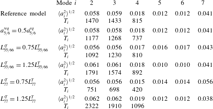The root mean squares of the amplitudes $a_{i}$ in the model are reported in table 2. Except for the last mode of the truncation, which is overestimated by a factor of four, a good agreement between the model and the DNS, within 30 %, is observed. We note that the modes retained in the seven-mode truncation represent only 63 % of the total combined kinetic and thermal energy.

Table 2.

Statistics of the modes integrated in the model over a period of 50 000 time units with noise (noise level 0.0012). Time $T_{i}$ is defined as the mean interval between zeros of $a_{i}^{\,f}$ , where $a_{i}^{f}$ is the filtered time series of $a_{i}$ obtained by moving average over two recirculation times (90 units). Intervals smaller than 90 units are excluded from the statistics.

Histories for the model amplitudes $a_{i}$ are presented in figure 9 over a period of 10 000 time units and compared with their counterparts in the DNS shown in figure 7. A good agreement is observed in the behaviour of the modes. The system spends long periods of time near the equilibria $|a_{2}|=|a_{2}^{eq}|$ , $|a_{3}|=|a_{3}^{eq}|$ , separated by switches from one diagonal to another, which correspond to individual sign changes of $a_{2}$ or  $a_{3}$ . We note that these sign changes can occasionally occur at the same time in the model (see around $t=2250$ and $t=3600$ in figure 9). Although this was not observed over the duration of the present DNS (which corresponds to a limited number of switches), simultaneous switches, i.e reversals along a given diagonal, were observed by Giannakis et al. (Reference Giannakis, Kolchinskaya, Krasnov and Schumacher2018). However, infrequent cessations of either mode 2 or 3 which were observed in the DNS are also present in the model: $a_{3}$ cancels around $t=6100$ or $a_{2}$ cancels around $t=8500$ . During these events, the LSC stabilizes in an $x$ or a $y$ plane (wall-parallel roll), even so this does not last more than 100 time units.

Figure 9.

Time evolution of the modelled POD coefficients. Each quasi-stable state is depicted by a different colour (same as in figure 7).

The coupling between the modes reported earlier in the DNS appears to be captured by the model. Firstly, as in the DNS, the amplitude of mode 4 is almost perfectly correlated in the model with the product $a_{2}a_{3}$ (the correlation coefficient is larger than 0.9 in both cases) and one has $a_{4}\sim Ca_{2}a_{3}$ , where $C\sim 5$ in the model and $C\sim 6$ in the DNS. 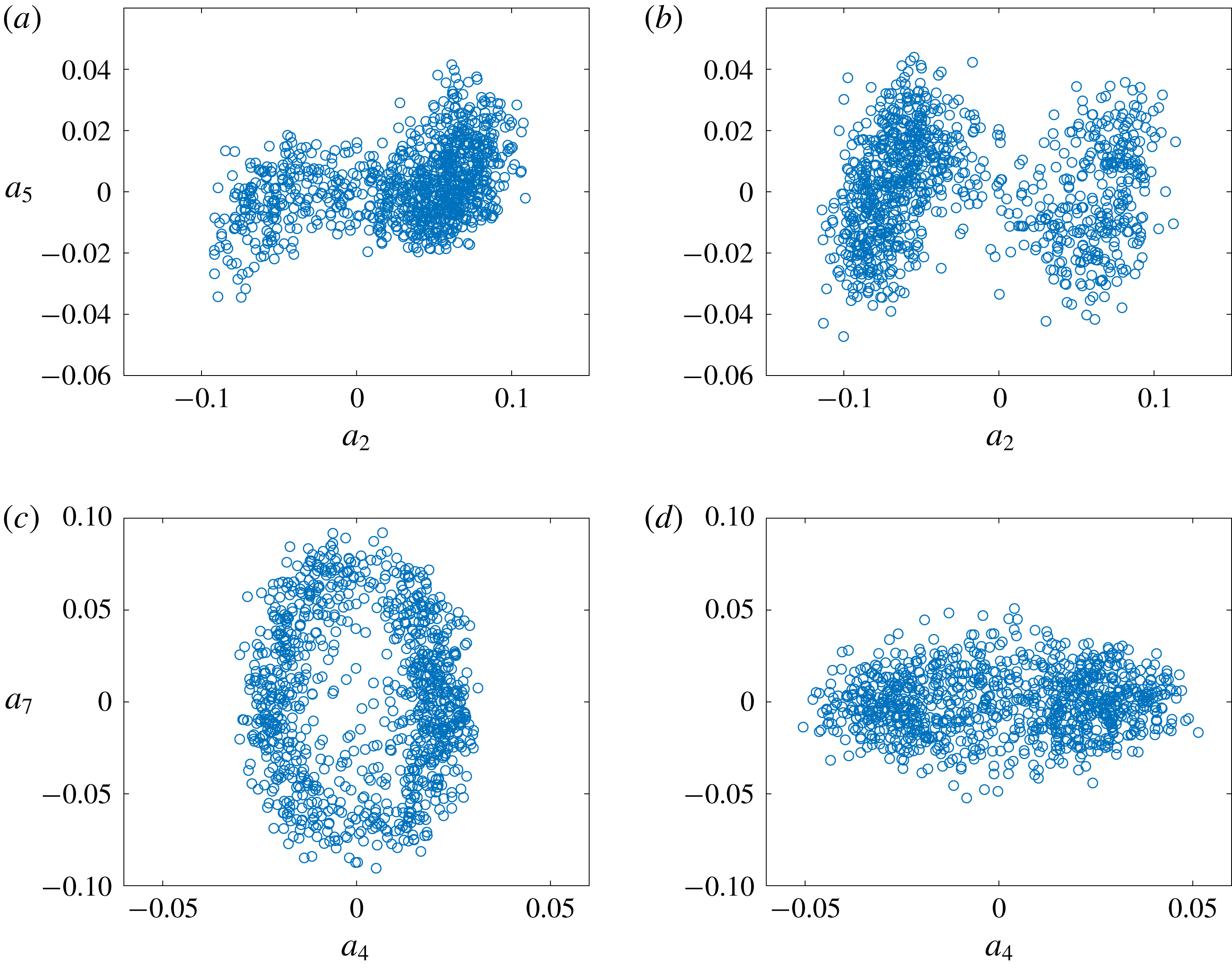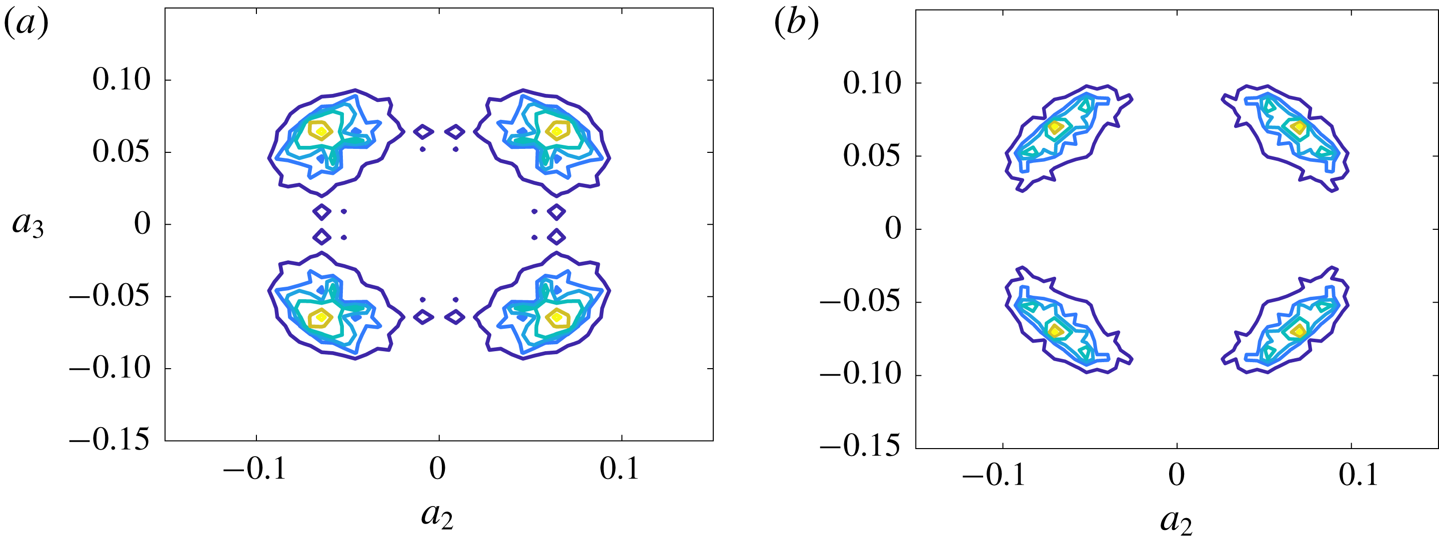Secondly, as in the DNS, figure 9 shows that although modes 5, 6 and 7 appear to fluctuate randomly on an individual basis, large excursions of the product $a_{5}a_{7}$ (respectively $a_{6}a_{7}$ ) tend to have the same sign as the opposite of $a_{2}$ (respectively $a_{3}$ ), which therefore indicates a connection between the interaction of these oscillating modes over long time scales and the state of the LSC. The agreement is confirmed by a comparison of phase portraits provided in figure 10. The dynamics of mode 2 and mode 5 is correctly captured by the model. As noted earlier, the amplitude of mode 7 is overestimated by the model but its qualitative behaviour appears to be correct. A 2-D histogram of modes 2 and 3 is compared with the DNS in figure 11: we note that unlike the phase portraits, symmetries were applied to the model as well as the DNS data. The agreement is good and confirms that the system spends most of its time near the diagonal states in both the model and the DNS.

Figure 10.

Phase portrait of the amplitudes in the model (a,c) and in the DNS (b,d). (a,b) $a_{2}$ and $a_{5}$ ; (c,d) $a_{4}$ and $a_{7}$ .

Figure 11.

Histogram in the $(a_{2},a_{3})$ space. (a) Model with noise amplitude $1.2\times 10^{-3}$ ; (b) DNS. Both DNS and model data are symmetrized. Isocontours $\{0.2;0.3;0.4;0.6;0.8;1\}$ .

4.2.2 Time scales

To characterize the times between the switches, we measure the times $T_{i},i\in \{2,3,4\}$ separating zeros of $a_{i}$ . Due to strong oscillations in the coefficients which could create numerical artefacts, we used a filtered version of the time series where a moving average over $T=90$ dimensionless time units was applied to $a_{i}$ . As mentioned earlier, this time scale represents a lower bound for the time required for a full diagonal switch and corresponds to two recirculation times. Values smaller than this time scale were therefore also excluded from the statistics. Results are given in table 2 and show that the model displays time scales between switches of the order of several hundred units, in good agreement with the DNS. We note that statistics for the DNS were obtained over a shorter period (10 000 time units) than the model, which was integrated over a longer period of time (50 000 time units). This accounts for the larger discrepancy between $T_{2}$ and $T_{3}$ observed in the DNS compared with the model.

Temporal spectra were computed for both the DNS and the model POD amplitudes. We checked that the time scales observed were independent of the time scale chosen for the noise signal in the model (10 dimensionless time units). Both sets were sampled at a resolution of 10 dimensionless time units. Results are shown in figure 12 for selected modes 2 and 7. Due to the long period between the switches relative to the total integration time, the characteristic time scale of switches is not clearly apparent in the spectra. A short time scale of 45 units can be identified in the DNS, versus a characteristic scale of about 110 in the model. This is larger by a factor of two than the recirculation time $T_{c}$ , which was identified in the DNS, but much less than the characteristic period between reorientations. Given the size of the truncation which captures only about 60 % of the combined energy, we can consider that the agreement is relatively satisfactory. The model is therefore able to exhibit both slow and fast dynamics on time scales comparable with those observed in the DNS.

Below the short time scale, one can notice on the spectra that remaining frequencies have higher amplitudes in the DNS compared with the model (this is also noticeable when comparing figures 7 and 9). This is not surprising given that the smallest spatial scales associated with the smallest time scales are only accounted for in the model through the addition of noise and one cannot expect to capture these temporal scales with a low-order truncation.

Figure 12.

Fourier transform modulus $|af_{i}|=|\hat{a}_{i}|$ of POD amplitudes in the model (a,c) and in the DNS (b,d). (a,b) $a_{2}$ ; (c,d) $a_{7}$ .

4.3 Physical interpretation of the model

4.3.1 Four-mode model

To understand the influence of the different modes, and in particular the higher-order ones, we consider a restriction of the model to the first four modes. The model has then the following form:

(4.17) $$\begin{eqnarray}\displaystyle & \displaystyle \frac{\text{d}a_{1}}{\text{d}t}=0, & \displaystyle\end{eqnarray}$$

(4.18) $$\begin{eqnarray}\displaystyle & \displaystyle \frac{\text{d}a_{2}}{\text{d}t}=\left(L_{22}^{T}-\unicode[STIX]{x1D6FC}_{22}\mathop{\sum }_{k=2}^{4}a_{k}a_{k}\right)\,a_{2}+0.29\,a_{1}a_{2}-0.53\,a_{3}a_{4}, & \displaystyle\end{eqnarray}$$

(4.19) $$\begin{eqnarray}\displaystyle & \displaystyle \frac{\text{d}a_{3}}{\text{d}t}=\left(L_{33}^{T}-\unicode[STIX]{x1D6FC}_{33}\mathop{\sum }_{k=2}^{4}a_{k}a_{k}\right)\,a_{3}+0.29\,a_{1}a_{3}-0.53\,a_{2}a_{4}, & \displaystyle\end{eqnarray}$$

(4.20) $$\begin{eqnarray}\displaystyle & \displaystyle \frac{\text{d}a_{4}}{\text{d}t}=\left(L_{44}^{T}-\unicode[STIX]{x1D6FC}_{44}\mathop{\sum }_{k=2}^{4}a_{k}a_{k}\right)\,a_{4}+0.48\,a_{4}a_{1}+1.06\,a_{2}a_{3}, & \displaystyle\end{eqnarray}$$

where $L_{22}^{T}=L_{33}^{T}$ and $\unicode[STIX]{x1D6FC}_{22}=\unicode[STIX]{x1D6FC}_{33}=\unicode[STIX]{x1D6FC}$ . As seen above, the model is characterized by four fixed points corresponding to the diagonal states $(a_{2}^{eq}=\pm a=\pm \sqrt{\unicode[STIX]{x1D706}_{2}},a_{3}^{eq}=\pm a=\pm \sqrt{\unicode[STIX]{x1D706}_{3}},a_{4}=\text{sgn}(a_{2}a_{3})\sqrt{\unicode[STIX]{x1D706}_{4}})$ observed in the DNS. It also displays four fixed pure (wall-parallel) roll states $(a_{2s}=\pm a_{s},a_{3}=a_{4}=0)$ and $(a_{2}=0,a_{3}=\pm a_{s},a_{4}=0)$ .

A remarkable feature of the four-mode model is that it reproduces the nearly perfect correlation between $a_{4}$ and $a_{2}a_{3}$ observed in the DNS. We therefore have

(4.21) $$\begin{eqnarray}a_{4}\sim Ca_{2}a_{3}\quad \text{with }C>0.\end{eqnarray}$$

This means that: (i) the effect of mode 4 is analogous to a feedback cubic term and (ii) the dynamics takes place on the centre manifold $a_{4}=Ca_{2}a_{3}$ , where the dynamical system can be written as

(4.22) $$\begin{eqnarray}\displaystyle & \displaystyle \frac{\text{d}a_{2}}{\text{d}t}=(\unicode[STIX]{x1D6FE}-\unicode[STIX]{x1D6FC}a_{2}^{2}-(\unicode[STIX]{x1D6FC}-\unicode[STIX]{x1D6FF})\,a_{3}^{2}-\unicode[STIX]{x1D6FC}C^{2}a_{2}^{2}a_{3}^{2})\,a_{2}, & \displaystyle\end{eqnarray}$$

(4.23) $$\begin{eqnarray}\displaystyle & \displaystyle \frac{\text{d}a_{3}}{\text{d}t}=(\unicode[STIX]{x1D6FE}-\unicode[STIX]{x1D6FC}a_{3}^{2}-(\unicode[STIX]{x1D6FC}-\unicode[STIX]{x1D6FF})\,a_{2}^{2}-\unicode[STIX]{x1D6FC}C^{2}a_{2}^{2}a_{3}^{2})\,a_{3}, & \displaystyle\end{eqnarray}$$

where $\unicode[STIX]{x1D6FF}=-0.53C$ and $\unicode[STIX]{x1D6FE}=L_{22/33}^{T}+0.29a_{1}$ . Stability analysis around the equilibria can then be performed in the $(a_{2},a_{3})$ subspace. For the diagonal equilibria, one has $\unicode[STIX]{x1D6FE}-(2\unicode[STIX]{x1D6FC}-\unicode[STIX]{x1D6FF})a^{2}-\unicode[STIX]{x1D6FC}C^{2}a^{4}=0$ , so that the Jacobian of the diagonal states $(\pm a,\pm a,\text{sgn}(a_{2}a_{3})Ca^{2})$ can be expressed as

(4.24) $$\begin{eqnarray}J_{d}^{2}=\left[\begin{array}{@{}cc@{}}-2\unicode[STIX]{x1D6FC}(1+C^{2}a^{2})a^{2} & -2(\unicode[STIX]{x1D6FC}-\unicode[STIX]{x1D6FF})a^{2}-2\unicode[STIX]{x1D6FC}C^{2}a^{4}\\ -2(\unicode[STIX]{x1D6FC}-\unicode[STIX]{x1D6FF})a^{2}-2\unicode[STIX]{x1D6FC}C^{2}a^{4} & -2\unicode[STIX]{x1D6FC}(1+C^{2}a^{2})a^{2}\\ \end{array}\right],\end{eqnarray}$$

which has two eigenvalues $-2\unicode[STIX]{x1D6FF}a^{2}$ and $2\unicode[STIX]{x1D6FF}a^{2}-4\unicode[STIX]{x1D6FC}(1+C^{2}a^{2})a^{2}$ . For a roll state defined by $a_{2}=\pm a_{s},a_{3}=a_{4}=0$ , one has $\unicode[STIX]{x1D6FE}-\unicode[STIX]{x1D6FC}a_{s}^{2}=0$ , and the associated Jacobian is

(4.25) $$\begin{eqnarray}J_{s}^{2}=\left[\begin{array}{@{}cc@{}}-2\unicode[STIX]{x1D6FC}a_{s}^{2} & 0\\ 0 & \unicode[STIX]{x1D6FF}a_{s}^{2}\\ \end{array}\right].\end{eqnarray}$$

An equivalent formulation is found for $(a_{2}=0,a_{3}=a_{s},a_{4}=0)$ by switching the two rows.

The stability of the roll states and the diagonal states therefore depends on the sign of $\unicode[STIX]{x1D6FF}=-0.53C$ . For $\unicode[STIX]{x1D6FF}<0$ , which corresponds to the Galerkin projection, the diagonal states are unstable and the roll states are stable (all eigenvalues are negative). However, the DNS corresponds to the situation where the roll states are unstable and the diagonal states are stable, i.e. the case $\unicode[STIX]{x1D6FF}>0$ (or equivalently a positive quadratic interaction between modes 2, 3 and 4). The addition of higher-order modes is therefore necessary to capture the correct dynamics.

4.3.2 Linear stability analysis of the full model

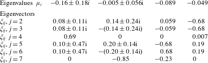
To investigate the influence of the modes in more detail, we study the stability of the diagonal equilibria in the full model. Table 3 shows the eigenvalues $\unicode[STIX]{x1D707}_{i}$ and eigenvectors $\text{}\underline{\unicode[STIX]{x1D709}}_{i}$ expressed in the basis of modes $a_{j}$ . Eigenvectors are either symmetric or antisymmetric with respect to $a_{2},a_{3},a_{5},a_{6}$ and are respectively orthogonal to $a_{7}$ or to $a_{4}$ . All equilibria are stable in the model. The most stable mode ( $\unicode[STIX]{x1D707}=-0.16\pm 0.18i$ ) contains predominantly mode $a_{4}$ and has no component along $a_{7}$ . In contrast, the least stable eigenmode ( $\unicode[STIX]{x1D707}=-0.005\pm 0.056\text{i}$ ) has a strong component in $a_{7}$ , confirming the destabilizing potential of the corner flow, in agreement with other observations (Giannakis et al. Reference Giannakis, Kolchinskaya, Krasnov and Schumacher2018). This least stable eigenvalue has an imaginary part of about $0.05$ , which corresponds to the characteristic time scale of about 110 found in the dynamics of the model.

Table 3.

Linear stability eigenvalues $\unicode[STIX]{x1D707}_{i}$ of the system around the equilibrium $(a1,a_{2}^{eq},a_{3}^{eq},a_{4}^{eq},a_{5}^{eq},a_{6}^{eq},0)$ and eigenvectors $\unicode[STIX]{x1D743}_{i}$ expressed in the basis $(a_{i},2\leqslant i\leqslant 7)$ .

4.3.3 Sensitivity of the model

Another way to understand the role played by the different modes is to study the effect of changes in the parameters of the model. Table 4 compares the statistics of the POD amplitudes when small changes are applied to the model coefficients. Other parameters such as the initial condition and the noise signal used to compute the reference statistics are kept the same. The cubic terms were also kept constant when adjusting the linear terms since they were not found to affect significantly the model dynamics. Results were confirmed by linear stability analysis.

The first case in table 4 corresponds to a scenario where the intensities of modes 5 and 6 at equilibria are decreased by half, which corresponds to an equivalent decrease in the coupling term $X_{5/6}$ (see appendix A). Physically this means that the connection between the LSC and the boundary layer is less intense, and we would expect the equilibrium to be less stable, leading to a decrease in the inter-switch mean time. This is indeed what is observed in the model. We then examine the effect of modifying the linear terms $L^{T}$ in the equations for modes 5 and 6, which is equivalent to adjusting the coupling terms $X_{5/6}$ (see appendix A). Given the energy ratio between mode 2 and mode 5 (respectively mode 3 and mode 6), it is clear that a moderate change in the linear term $L_{52/63}^{T}$ will correspond to a larger modification of the diagonal term $L_{55/66}^{T}$ . Table 4 shows that for a decrease in $L_{55/66}^{T}$ ( $L_{55/66}^{T}$ is negative), the time between switches increases, the energy in modes 2 and 3 increases, while that in modes 5 and 6 decreases. The energy in mode 4 remains about constant. The trends are opposite for an increase in $L_{55/66}^{T}$ . This supports the idea that increasing the energy transfer to the boundary-layer modes 5 and 6 leads to more destabilization associated with a higher energy content in these modes. The behaviour of the model therefore highlights the importance of the boundary-layer modes for the reorientation process.

Similarly, table 4 shows that a decrease in $L_{77}^{T}$ ( $L_{77}^{T}$ is negative) leads to an increase of the time between switches, and a decrease in the energy of mode 7, along with an increase in the energy of modes 2, 3 as well as mode 4. The energy of modes 5 and 6 does not appear to change significantly. The trends are reversed for an increase in $L_{77}^{T}$ . The importance of mode 7 for the destabilization process is therefore confirmed. The changes in the inter-switch periods due to modifications in $L_{77}^{T}$ are stronger than those observed for $L_{55/66}^{T}$ .

Table 4.

Statistics of the integrated modes for slight variations of the model coefficients. The noise level is $1.2\times 10^{-3}$ .