1 Introduction
In most suspensions, particles are non-spherical or even irregular (Yang et al. Reference Yang, Kim, Lim and Yi2008; Bagheri et al. Reference Bagheri, Bonadonna, Manzella and Vonlanthen2015) with no symmetry, e.g., asphaltenes clusters in heavy crude oil (Mullins et al. Reference Mullins, Sheu, Hammami and Marshall2007), crystal particles in magma and melts (Mader, Llewellin & Mueller Reference Mader, Llewellin and Mueller2013), and metal oxides clusters (Rubio-Hernández et al. Reference Rubio-Hernández, Ayucar-Rubio, Velazquez-Navarro and Galindo-Rosales2006), among others. The irregular geometry of particles strongly affects the particle–fluid and particle–particle interactions, and consequently complicates the flow structure (Qi & Luo Reference Qi and Luo2003). However, shapes of particles are typically approximated by simplified geometries, such as spheres, ellipsoids, rods, disks, etc., in the numerical/theoretical analysis of rheology (Carrasco & de la Torre Reference Carrasco and de la Torre1999; Martys Reference Martys2005; Pabst, Gregorová & Berthold Reference Pabst, Gregorová and Berthold2006; Rubio-Hernández et al. Reference Rubio-Hernández, Ayucar-Rubio, Velazquez-Navarro and Galindo-Rosales2006; Lindström & Uesaka Reference Lindström and Uesaka2009; Mader et al. Reference Mader, Llewellin and Mueller2013; Denn & Morris Reference Denn and Morris2014; Pal Reference Pal2015) or to obtain microstructure information from bulk rheology measurements (Eyssautier, Frot & Barré Reference Eyssautier, Frot and Barré2012; Ghanavati, Shojaei & Ahmad Ramazani Reference Ghanavati, Shojaei and Ahmad Ramazani2013). The main question is if the current methods of defining equivalent particles (see § 2.4) work well for suspensions of irregular particles.
The earliest attempt to solve a suspension of non-spherical particles is the pioneering work of Jeffery (Reference Jeffery1922) for ellipsoidal particles. Jeffery provided an analytical solution for the time evolution of a particle’s orientation in the absence of inertial and Brownian motion effects, which is now referred to as Jeffery’s orbit. Hinch & Leal (Reference Hinch and Leal1979) obtained a solution for rotation of a non-axisymmetric triaxial ellipsoid in terms of Euler angles. They discussed a small departure from axisymmetry for ellipsoidal particles and showed that the motion is composed of a rapid rotation around Jeffery orbits, and a slower periodic drift leading to a change of orbit. Using a Stokesian solution for the dynamic orientation of non-Brownian triaxial ellipsoids, Yarin, Gottlieb & Roisman (Reference Yarin, Gottlieb and Roisman1997) found that, for sufficiently long ellipsoids, particles may rotate in a chaotic manner.
Bretherton (Reference Bretherton1962) extended the work of Jeffery for more general shapes and observed that almost all axially symmetric particles will rotate according to Jeffery’s orbit. Brenner (Reference Brenner1974) later showed that, for an arbitrary axisymmetric particle in a dilute Newtonian suspension, the particle’s contribution to the total stress tensor can be formulated as a function of volume fraction, viscosity of the solvent, deformation rate tensor, second- and fourth-order orientation tensors and five constants: four shape constants and one rotary diffusivity due to Brownian motion (for large enough particles Brownian motion can be neglected). In fact, these five dimensionless scalars, which depend only on the shape of the particle, suffice to fully determine the hydrodynamic interaction between the particle and the liquid in Stokesian dynamics (Petrie Reference Petrie1999).
Fibre suspensions are amongst the most studied class of non-spherical particle suspensions due to great theoretical interest and numerous industrial applications (Shaqfeh & Fredrickson Reference Shaqfeh and Fredrickson1990; Petrie Reference Petrie1999; Chaouche & Koch Reference Chaouche and Koch2001; Pabst et al. Reference Pabst, Gregorová and Berthold2006; Lindström & Uesaka Reference Lindström and Uesaka2009). The modelling approach considers all fibres as straight circular cylinders with uniform length and diameter. The fibre aspect ratio (length over diameter) is high, and typically ranges from 10 to 1000 (Chinesta & Ausias Reference Chinesta and Ausias2015). There have been both theoretical and empirical relations obtained for the effective (equivalent) aspect ratio for rod-like particles based on Jeffery’s orbital solution (Mason & Manley Reference Mason and Manley1956; Nawab & Mason Reference Nawab and Mason1958; Harris & Pittman Reference Harris and Pittman1975; Burgers Reference Burgers1995). Due to the high aspect ratio, another asymptotic technique, called slender-body theory, can also be used to obtain analytical approximations for the Stokes flow around fibres (Batchelor Reference Batchelor1970). Batchelor (Reference Batchelor1971), with this technique, developed a new model (referred to as the cell model) to derive the stress generated by slender rods in a pure strain flow at up to semidilute volume fractions, considering hydrodynamic interactions between fibres. Batchelor’s model was later extended to more generalized particle orientations and flow characteristics, resulting in different shape coefficients for the stress tensor (Dinh & Armstrong Reference Dinh and Armstrong1984; Chung & Kwon Reference Chung and Kwon1996). For suspensions of high-aspect-ratio fibre, Shaqfeh & Fredrickson (Reference Shaqfeh and Fredrickson1990) developed a theoretical description for the hydrodynamic interactions based on multiple scattering. By including many multiparticle interactions, their theory for semidilute suspensions enhanced the cell model of Dinh & Armstrong (Reference Dinh and Armstrong1984).
All the above Stokesian solutions are available for regular geometries (axisymmetric or non-axisymmetric particles such as triaxial ellipsoids). For more complicated particle shapes, however, numerical techniques are required to study the particle motion in a suspension or calculate the rheological parameters. One difficulty with numerical simulations for suspensions of non-spherical particles, however, comes from the solution of the coupled governing equations for the flow and the immersed particles at the geometrically complex boundaries. Youngren & Acrivos (Reference Youngren and Acrivos1975) formulated the problem of slow viscous flow of an unbounded fluid past a single solid particle as a system of linear integral equations of the first kind, in which the surface-stress force could be obtained numerically by reducing the integral equations to a system of linear algebraic equations. Karrila, Fuentes & Kim (Reference Karrila, Fuentes and Kim1989) presented an iterative algorithm to solve the kinematics and stresslet of a multiparticle suspension of arbitrary shapes in Stokes flow when the total forces and torques acting on particles are given. The linear Stokes equation resolves the motion of particles and hydrodynamics of flow by solving a system of linear algebraic equations (Claeys & Brady Reference Claeys and Brady1993; Kumar & Higdon Reference Kumar and Higdon2011a ), which is much cheaper in terms of computational costs compared to the nonlinear Navier–Stokes equations.
In many applications, the inertia of the solid particles and the unsteady inertia of the fluid is sufficiently large that it can change the characteristics of the particles’ motion (Feng & Joseph Reference Feng and Joseph1995). For instance, experimental studies (Karnis, Goldsmith & Mason Reference Karnis, Goldsmith and Mason1963, Reference Karnis, Goldsmith and Mason1966) on rods and disks showed that even weak fluid inertia is sufficient to force non-spherical particles to drift towards an orientation that is different from a Jeffery’s orbit. For suspensions with weak (but not negligible) fluid inertia, the analytical approach typically uses a perturbation expansion method to the Stokes solution (Subramanian & Koch Reference Subramanian and Koch2005, Reference Subramanian and Koch2006; Einarsson et al.
Reference Einarsson, Candelier, Lundell, Angilella and Mehlig2015; Dabade, Marath & Subramanian Reference Dabade, Marath and Subramanian2016). Even though these analytical solutions provide great insight into the orientational dynamics and rheology of suspensions, they pertain only to simple geometries such as spheroids (Einarsson et al.
Reference Einarsson, Candelier, Lundell, Angilella and Mehlig2015; Dabade et al.
Reference Dabade, Marath and Subramanian2016) or are limited to special cases such as fibres with very long aspect ratios (Subramanian & Koch Reference Subramanian and Koch2005) or nearly spherical particles (Subramanian & Koch Reference Subramanian and Koch2006). Moreover, these asymptotic solutions are only accurate for very weak inertia (
 $Re\ll 1$
). The latter limitation has been resolved by implementing numerical simulations and the development of massively parallel computing platforms. Applying the lattice Boltzmann method, dynamics of spheroids and rods (two common non-spherical particles) has been extensively analysed for various ranges of fluid and particle inertia (Aidun, Lu & Ding Reference Aidun, Lu and Ding1998; Qi & Luo Reference Qi and Luo2003; Ku & Lin Reference Ku and Lin2009; Mao & Alexeev Reference Mao and Alexeev2014; Rosén, Lundell & Aidun Reference Rosén, Lundell and Aidun2014; Rosén et al.
Reference Rosén, Do-Quang, Aidun and Lundell2015a
,Reference Rosén, Do-Quang, Aidun and Lundell
b
,Reference Rosén, Einarsson, Nordmark, Aidun, Lundell and Mehlig
c
).
The above studies have shed light on the rheology of a suspension of non-spherical particles, but they are restricted to regular geometries. Our objective is to evaluate the accuracy of approximating the shape of irregular particles with equivalent regular ones in different suspensions. In this paper, two random, yet very different irregular particles are chosen and compared with equivalent simple geometries. One particle is solid with skewed sharp edges but without any hole, while the other one is of more slender shape with some holes. We used our well-validated numerical framework (§ 2), to study the motion of particles (§ 3) and the particle stress (§ 4.1), and investigate the role of shape factors on rheological parameters (intrinsic viscosity and normal stress differences in §§ 4.2 and 5, respectively) by comparing our results with equivalent spheres and spheroids.
2 Method and material
2.1 Numerical framework: structure/flow solvers and three-dimensional rigid body rotation
The numerical method used to simulate the motion of neutrally buoyant particles in the shear flow is the curvilinear immersed boundary (CURVIB) method (Gilmanov & Sotiropoulos Reference Gilmanov and Sotiropoulos2005; Ge & Sotiropoulos Reference Ge and Sotiropoulos2007; Borazjani, Ge & Sotiropoulos Reference Borazjani, Ge and Sotiropoulos2008), which is coupled with the rigid body dynamics of moving particles (Daghooghi & Borazjani Reference Daghooghi and Borazjani2015b ). These solvers are coupled together through a strong coupling with under-relaxation approach (Borazjani et al. Reference Borazjani, Ge and Sotiropoulos2008). Details of the computational method and the validations for rheology can be found in our previous publication (Daghooghi & Borazjani Reference Daghooghi and Borazjani2015b ), and only a brief overview is provided in what follows.
The motion of each particle is calculated by solving the linear and angular momentum equations around its centre of mass (Daghooghi & Borazjani Reference Daghooghi and Borazjani2015b ). Instead of the conventional way of solving for the time evolution of the rotation matrix with Euler angles for angular momentum equations, we use quaternions to represent the orientation of the body in the three-dimensional space (Daghooghi & Borazjani Reference Daghooghi and Borazjani2015b ) to avoid the numerical drift (Baraff Reference Baraff1997). The hydrodynamic moment and force exerted on each particle, needed to solve the linear and angular momentum equations, are calculated based on the pressure and flow field (from the flow solver) around each particle at any time instant (Daghooghi & Borazjani Reference Daghooghi and Borazjani2015b ).
The equations governing the fluid motion are the unsteady three-dimensional (3-D) Navier–Stokes equations. Governing equations are non-dimensionalized by a characteristic velocity
 $\dot{\unicode[STIX]{x1D6FE}}\mathfrak{L}$
and a characteristic length
 $\mathfrak{L}$
(one-half the largest diameter of the particle) and discretized using a hybrid staggered/non-staggered approach with QUICK and central schemes for convective and viscous terms, respectively (Gilmanov & Sotiropoulos Reference Gilmanov and Sotiropoulos2005). To handle the moving boundaries, a sharp-interface immersed boundary method is used (Gilmanov & Sotiropoulos Reference Gilmanov and Sotiropoulos2005; Ge & Sotiropoulos Reference Ge and Sotiropoulos2007; Borazjani et al.
Reference Borazjani, Ge and Sotiropoulos2008). Using the strong-coupling partitioned approach with under-relaxation (Borazjani et al.
Reference Borazjani, Ge and Sotiropoulos2008), we solve the fluid and structured domain together. In this method, the fluid and structure domains are separately advanced in time, but the simultaneous (implicit) solution of both equations is achieved through fluid/structure sub-iterations (Daghooghi & Borazjani Reference Daghooghi and Borazjani2015b
). The method has been extensively validated for a variety of complex flow problems (Borazjani et al.
Reference Borazjani, Ge, Le and Sotiropoulos2013; Asgharzadeh & Borazjani Reference Asgharzadeh and Borazjani2017) and successfully implemented in various applications such as rheology of suspensions (Daghooghi & Borazjani Reference Daghooghi and Borazjani2015b
), aquatic motions (Daghooghi & Borazjani Reference Daghooghi and Borazjani2015a
; Bottom II et al.
Reference Bottom, Borazjani, Blevins and Lauder2016; Daghooghi & Borazjani Reference Daghooghi and Borazjani2016), cardiovascular flows (Hedayat, Asgharzadeh & Borazjani Reference Hedayat, Asgharzadeh and Borazjani2017) and active suspensions (Daghooghi & Borazjani Reference Daghooghi and Borazjani2017), among others.
2.2 Formulation of rheological parameters
The last step in our numerical framework is the calculation of the particle stress from the simulated motion of fluid and particles. Note that all the parameters reported in the work are non-dimensional parameters which are non-dimensionalized by a combination of density
 $\unicode[STIX]{x1D70C}$
, characteristic length
 $\mathfrak{L}$
(one-half the largest diameter of the particle), and characteristic velocity
 $\dot{\unicode[STIX]{x1D6FE}}\mathfrak{L}$
. The volume average of stress (non-dimensionalized by
 $\unicode[STIX]{x1D70C}\dot{\unicode[STIX]{x1D6FE}}^{2}\mathfrak{L}^{2}$
) in a statistically homogeneous suspension is calculated as (Batchelor Reference Batchelor1970):
 $$\begin{eqnarray}\unicode[STIX]{x1D6F4}_{ij}=-\unicode[STIX]{x1D6FF}_{ij}\frac{1}{V}\int _{V_{f}}p\,\text{d}V+\unicode[STIX]{x1D707}\left(\frac{\unicode[STIX]{x2202}{\mathcal{U}}_{i}}{\unicode[STIX]{x2202}x_{j}}+\frac{\unicode[STIX]{x2202}{\mathcal{U}}_{j}}{\unicode[STIX]{x2202}x_{i}}\right)+\unicode[STIX]{x1D6F4}_{ij}^{p},\end{eqnarray}$$
where
 $p$
is the pressure (non-dimensionalized by
 $\unicode[STIX]{x1D70C}\dot{\unicode[STIX]{x1D6FE}}^{2}\mathfrak{L}^{2}$
),
 $V$
and
 $V_{f}$
are the total volume of suspension and the volume occupied by the fluid (non-dimensionalized by
 $\mathfrak{L}^{3}$
), respectively, and
 $\unicode[STIX]{x2202}{\mathcal{U}}_{i}/\unicode[STIX]{x2202}x_{j}$
is the volume-averaged velocity gradient (non-dimensionalized by
 $\dot{\unicode[STIX]{x1D6FE}}$
).
 $\unicode[STIX]{x1D6F4}_{ij}^{p}$
is the particle stress and represents the contribution to the bulk stress due to the presence of particles (Batchelor Reference Batchelor1970). For rigid particles, this contribution reads as follows:
 $$\begin{eqnarray}\unicode[STIX]{x1D6F4}_{ij}^{p}=\frac{1}{V}\mathop{\sum }_{n=1}^{N}\int _{(A_{p})_{n}}x_{j}\unicode[STIX]{x1D70E}_{ik}n_{k}\,\text{d}A-\frac{1}{V}\mathop{\sum }_{n=1}^{N}\int _{(V_{p})_{n}}\unicode[STIX]{x1D70C}x_{j}a_{i}\,\text{d}V-\frac{1}{V}\int _{V}\unicode[STIX]{x1D70C}u_{i}^{\prime }u_{j}^{\prime }\,\text{d}V,\end{eqnarray}$$
where
 $A_{p}$
and
 $V_{p}$
are the particle’s dimensionless surface area and volume (non-dimensionalized by
 $\mathfrak{L}^{2}$
and
 $\mathfrak{L}^{3}$
), respectively,
 $N$
is the total number of particles in the suspension,
 $\unicode[STIX]{x1D70E}_{ik}$
is the Newtonian stress,
 $u_{i}^{\prime }$
are velocity fluctuations,
 $x_{i}$
is the displacement vector measured from the particle’s centre of mass (choice of the reference point is arbitrary), and
 $a_{i}$
is the particle acceleration. In the absence of external torque on particles, the symmetric part of the particle stress is given by:
 $$\begin{eqnarray}\unicode[STIX]{x1D6F4}_{ij}^{p,s}=\frac{1}{V}\mathop{\sum }_{n=1}^{N}(\unicode[STIX]{x1D61A}_{ij})_{n}-\mathop{\sum }_{n=1}^{N}(\unicode[STIX]{x1D617}_{ij})_{n}-\unicode[STIX]{x1D619}_{ij},\end{eqnarray}$$
where
 $\unicode[STIX]{x1D61A}_{ij}$
is stresslet (Batchelor Reference Batchelor1970),
 $\unicode[STIX]{x1D617}_{ij}$
is the acceleration stress, and
 $\unicode[STIX]{x1D619}_{ij}$
is the Reynolds stress. Neglecting Brownian effects for a suspension consisting of neutrally buoyant rigid particles of arbitrary shape, these terms are as follows:
 $$\begin{eqnarray}\displaystyle & \displaystyle \unicode[STIX]{x1D61A}_{ij}=\int _{A_{p}}\frac{1}{2}(\unicode[STIX]{x1D70E}_{ik}x_{j}+\unicode[STIX]{x1D70E}_{jk}x_{i})n_{k}\,\text{d}A, & \displaystyle\end{eqnarray}$$
 $$\begin{eqnarray}\displaystyle & \displaystyle \unicode[STIX]{x1D617}_{ij}=\frac{1}{V}\int _{V_{p}}\frac{1}{2}(a_{i}x_{j}+a_{j}x_{i})\,\text{d}V, & \displaystyle\end{eqnarray}$$
 $$\begin{eqnarray}\displaystyle & \displaystyle \unicode[STIX]{x1D619}_{ij}=\frac{1}{V}\int _{V}(u_{i}^{\prime }u_{j}^{\prime })\,\text{d}V, & \displaystyle\end{eqnarray}$$
 $\unicode[STIX]{x1D64E}$
is non-dimensionalized with respect to
 $\unicode[STIX]{x1D70C}\dot{\unicode[STIX]{x1D6FE}}^{2}\mathfrak{L}^{5}$
,
 $\unicode[STIX]{x1D64B}$
and
 $\unicode[STIX]{x1D64D}$
are non-dimensionalized with respect to
 $\unicode[STIX]{x1D70C}\dot{\unicode[STIX]{x1D6FE}}^{2}\mathfrak{L}^{2}$
, and all variables on the right-hand side of (2.4) are non-dimensional variables from fluid and structure solvers. It should be noted that the antisymmetric part of the particle stress (directly related to the torque on each particle) is not zero at any instance of time. This is due to the fact that we have not neglected the inertia. In Stokesian dynamics (suspended particles are both force-free and torque-free), only stresslet term (2.4a
) should be considered. Two other terms of (2.3) extend this framework to non-zero
 $Re$
(Aidun & Clausen Reference Aidun and Clausen2010). Finally, normal stress differences and the relative viscosity are defined by (Guazzelli & Morris Reference Guazzelli and Morris2011):
 $$\begin{eqnarray}\displaystyle & \displaystyle N_{1}=\bar{\unicode[STIX]{x1D6F4}}_{zz}^{p,s}-\bar{\unicode[STIX]{x1D6F4}}_{yy}^{p,s}=\frac{1}{V}\mathop{\sum }_{n=1}^{N}(\bar{\unicode[STIX]{x1D61A}}_{zz}-\bar{\unicode[STIX]{x1D61A}}_{yy})_{n}-\mathop{\sum }_{n=1}^{N}(\bar{\unicode[STIX]{x1D617}}_{zz}-\bar{\unicode[STIX]{x1D617}}_{yy})_{n}-(\bar{\unicode[STIX]{x1D619}}_{zz}-\bar{\unicode[STIX]{x1D619}}_{yy}) & \displaystyle\end{eqnarray}$$
 $$\begin{eqnarray}\displaystyle & \displaystyle N_{2}=\bar{\unicode[STIX]{x1D6F4}}_{yy}^{p,s}-\bar{\unicode[STIX]{x1D6F4}}_{xx}^{p,s}=\frac{1}{V}\mathop{\sum }_{n=1}^{N}(\bar{\unicode[STIX]{x1D61A}}_{yy}-\bar{\unicode[STIX]{x1D61A}}_{xx})_{n}-\mathop{\sum }_{n=1}^{N}(\bar{\unicode[STIX]{x1D617}}_{yy}-\bar{\unicode[STIX]{x1D617}}_{xx})_{n}-(\bar{\unicode[STIX]{x1D619}}_{yy}-\bar{\unicode[STIX]{x1D619}}_{xx}) & \displaystyle\end{eqnarray}$$
 $$\begin{eqnarray}\displaystyle & \displaystyle \unicode[STIX]{x1D702}_{r}=1+Re\bar{\unicode[STIX]{x1D6F4}}_{yz}^{p,s}=1+Re\left[\frac{1}{V}\mathop{\sum }_{n=1}^{N}(\bar{\unicode[STIX]{x1D61A}}_{yz})_{n}-\mathop{\sum }_{n=1}^{N}(\bar{\unicode[STIX]{x1D617}}_{yz})_{n}-\bar{\unicode[STIX]{x1D619}}_{yz}\right], & \displaystyle\end{eqnarray}$$
 $\overline{\bullet }$
denotes the average value of
 $\bullet$
, and
 $(x,y,z)$
correspond to vorticity, velocity gradient and flow directions, respectively, as will be shown in figure 3. We have implemented and verified the calculation of these rheological parameters in our numerical framework by comparing the numerical values against available analytical solutions in our previous work (Daghooghi & Borazjani Reference Daghooghi and Borazjani2015b
).
2.3 Computational set-up and irregular-shaped particles
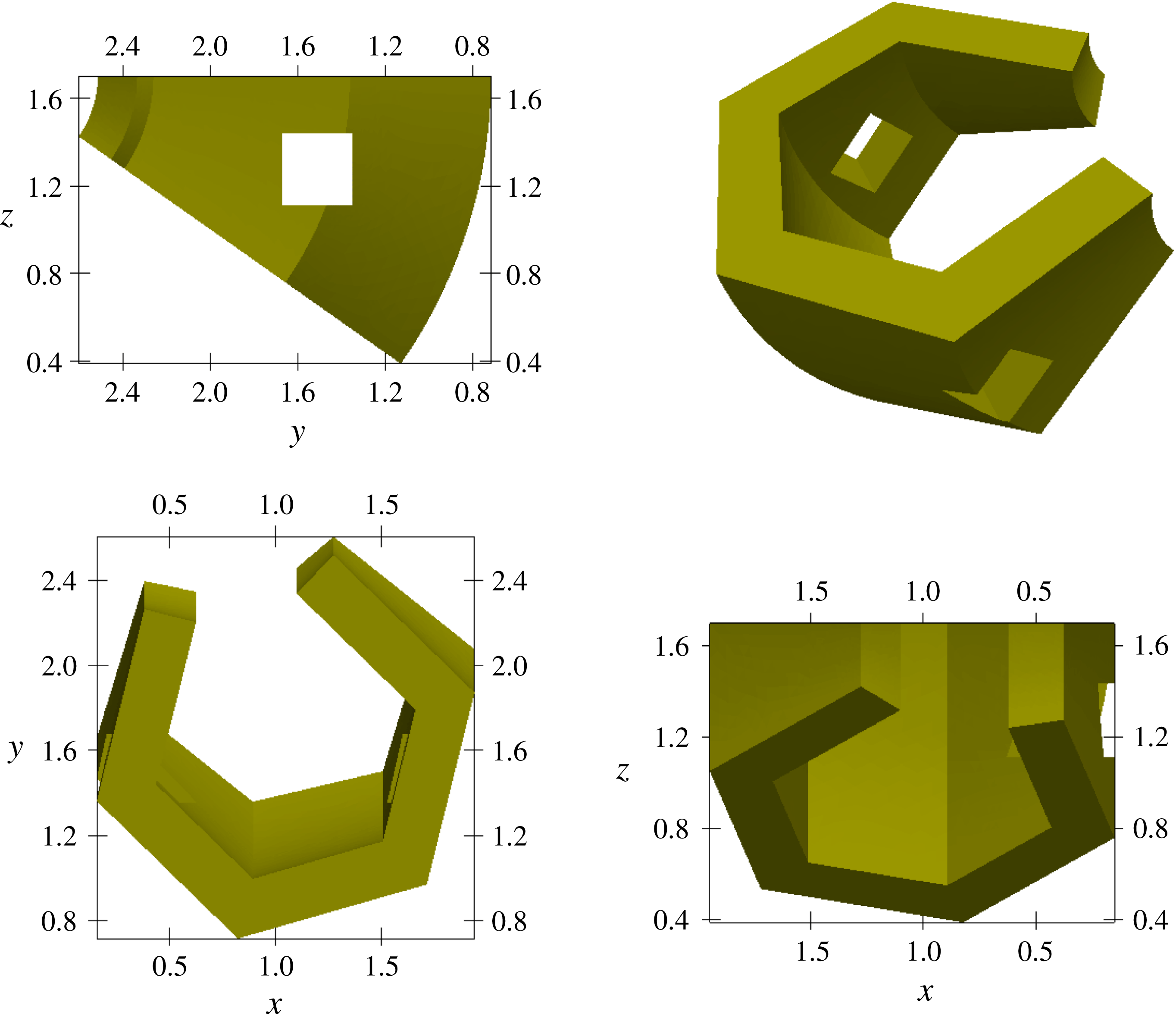
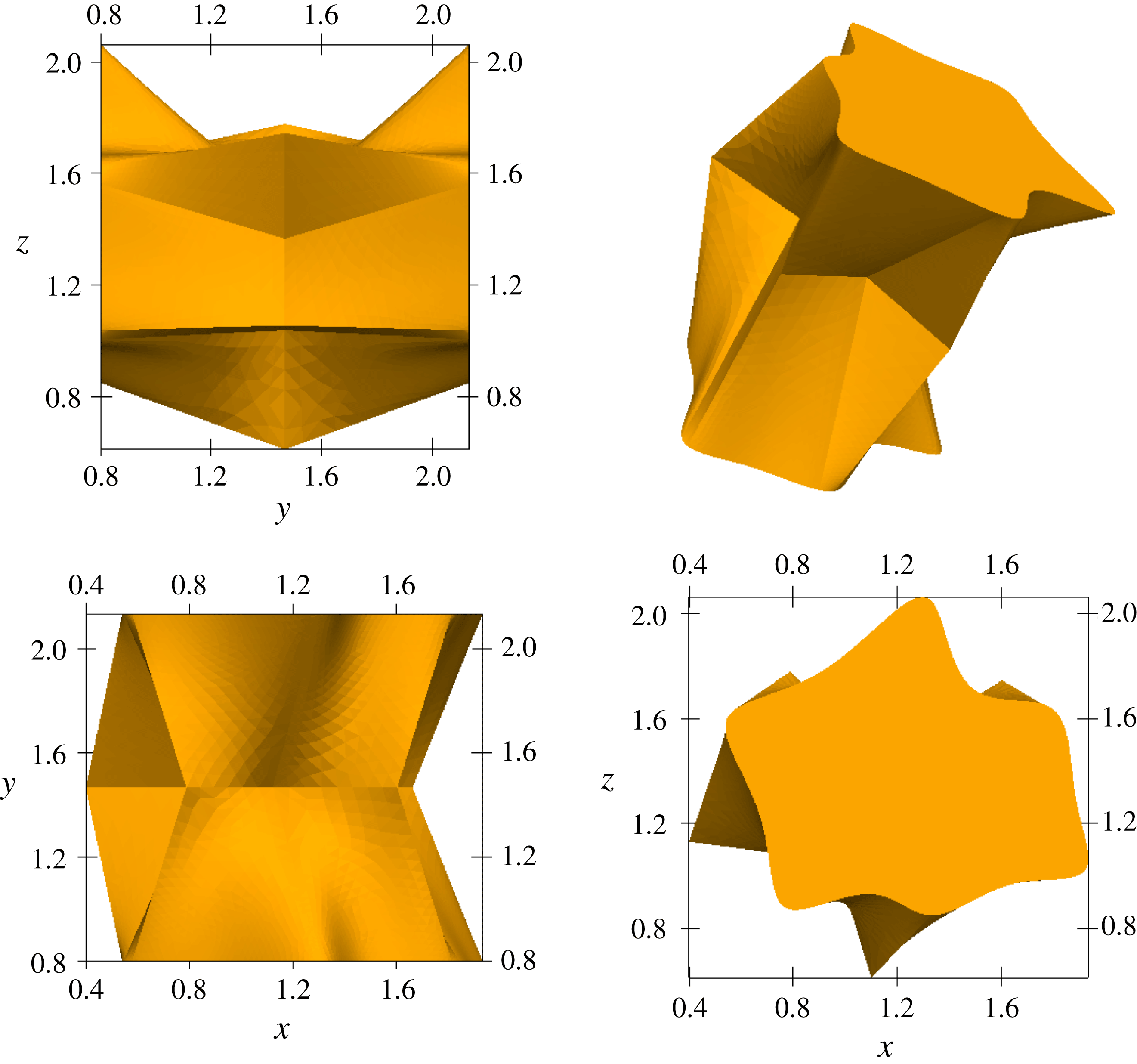
To investigate the effect of irregular shape of particles, we picked two different arbitrary irregular particles: (1) particle
 $\beth$
, which is a slender curved particle with holes inside; and (2) particle
 $\aleph$
, which is a solid particle with skewed sharp edges. The schematics of these particles in a 3-D view and projection of each particle on Cartesian coordinate planes with correlated scales are shown in figures 1 and 2.
A 3-D view and projections of particle
 $\beth$
on Cartesian coordinate planes with correlated scales are shown.
 $\beth$
is a slender curved particle with holes inside, which has a surface-to-volume ratio of 11.4.

A 3-D view and projections of particle
 $\aleph$
on Cartesian coordinate planes with correlated scales are shown.
 $\aleph$
is a solid particle with skewed sharp edges, which has a surface-to-volume ratio of 7.4.

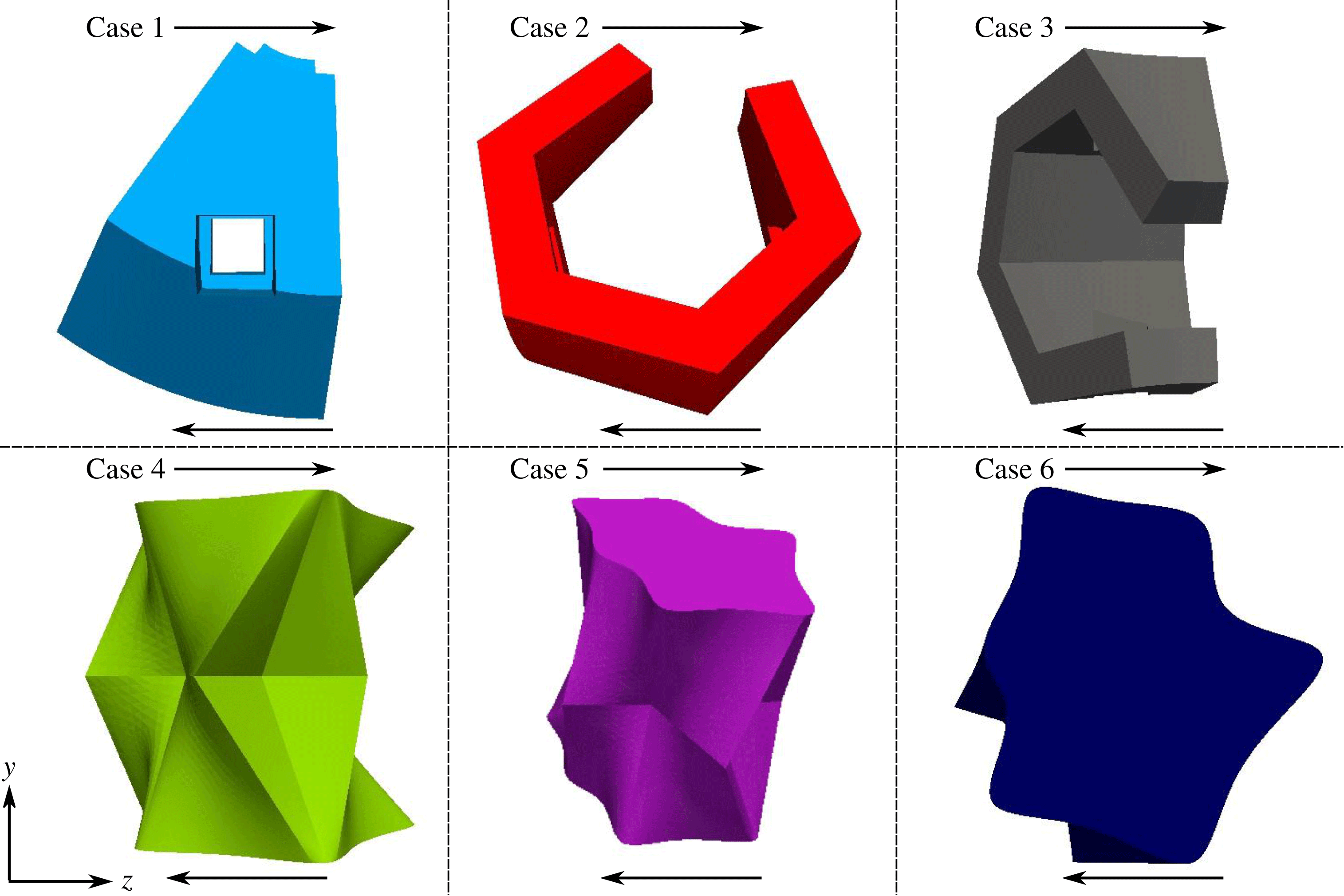
Unlike particles with principal axis such as ellipsoids, for an irregular-shaped particle, there is no major axis (axis of symmetry) that can be used to define and distinguish different initial orientations. Therefore, we have to use random initial orientations. For each particle, we consider three cases with different initial orientations. For particle
 $\beth$
, we first initialized the geometry randomly and named it as case 1. Two more cases (case 2 and case 3) are obtained by rotating the first case by 90 degrees around
 $y$
- and
 $z$
-axes, respectively. Similarly, for particle
 $\aleph$
, case 4 is initialized using a random orientation. Case 5 and case 6 are obtained by rotating case 4 by 45 degrees with respect to the
 $(0,0.707,0.707)$
vector and 90 degrees with respect to the
 $z$
-axis. Figure 3 shows the schematic of all these cases at their initial orientations with respect to the background shear flow vorticity (out-of-plane) direction.
The computational set-up is similar to the one used in our previous work (Daghooghi & Borazjani Reference Daghooghi and Borazjani2015b
). The flow is initialized with a linear shear flow. Boundary conditions in the velocity gradient direction (
 $y$
-direction in figure 3) are moving walls in opposite directions, and other directions are set to be periodic. The implementation of periodic boundary conditions creates a planar array of particles that rotate in phase, i.e., a periodic suspension (Yu, Phan-Thien & Tanner Reference Yu, Phan-Thien and Tanner2007; Huang, Wu & Lu Reference Huang, Wu and Lu2012a
; Rosén et al.
Reference Rosén, Lundell and Aidun2014, Reference Rosén, Do-Quang, Aidun and Lundell2015a
,Reference Rosén, Do-Quang, Aidun and Lundell
b
,Reference Rosén, Einarsson, Nordmark, Aidun, Lundell and Mehlig
c
). Such simulations can be a good approximation of a homogeneous suspension in low concentrations in which particles are sufficiently far from each other and close–distance interactions are less likely to happen (Daghooghi & Borazjani Reference Daghooghi and Borazjani2015b
). Note that in a real suspension particles locate randomly and rotate with phase difference under shear, but the particle–particle interaction is low in dilute regimes. Meanwhile, this boundary condition is a better approximation compared to the far-field boundary condition that is considered in the analytical Stokes solution for dilute regimes (Daghooghi & Borazjani Reference Daghooghi and Borazjani2015b
). Based on grid sensitivity tests, the grid size is selected as
 $\unicode[STIX]{x1D6E5}=0.02\mathfrak{L}$
.
Schematic of different cases based on initial orientation. Case 1, case 2, and case 3 are constructed from particle
 $\beth$
and case 4, case 5, and case 6 are made from particle
 $\aleph$
. The arrows show the direction of shear flow around the particles.

In all cases investigated in this paper, volume fraction and Reynolds number are fixed at
 $\unicode[STIX]{x1D719}=0.058$
and
 $Re=1.0$
. These values are consistent with the assumption of a dilute suspension under the influence of inertia and also equal to corresponding values in our previous simulations for spheroids. This similarity enables us to compare our results with similar suspensions consisting of spheroids (Daghooghi & Borazjani Reference Daghooghi and Borazjani2015b
) and study the role of a particle’s shape.
2.4 Equivalent shape models for irregular particles
The definition of a regular shape is that it can be simplified by a few geometrical parameters, e.g., the diameter of a sphere (one dimension), the aspect ratio and the length of one axis of a prolate or oblate spheroid (two dimensions), or the semi-axis lengths of a triaxial ellipsoid (three dimensions) (Taylor et al. Reference Taylor, Garboczi, Erdogan and Fowler2006). An equivalent regular shape model for an irregular particle can be built based on either (1) measured geometrical properties of an irregular particle (Taylor et al. Reference Taylor, Garboczi, Erdogan and Fowler2006), or (2) its kinematics in the bulk flow (Mason & Manley Reference Mason and Manley1956; Harris & Pittman Reference Harris and Pittman1975).
In the geometrical approach, one or more geometrical properties such as volume or surface are selected and measured. The equivalent regular shape is then picked such that it has the same selected geometrical properties as the irregular one. One of the most frequent one-parameter models (simplest model) is an equivalent volume sphere, whose diameter is determined by forcing the sphere to have the same volume as the irregular particle (Taylor et al. Reference Taylor, Garboczi, Erdogan and Fowler2006). For particles with lower sphericity (Bullard & Garboczi Reference Bullard and Garboczi2013), oblate or prolate spheroids with closest aspect ratios are commonly used in experimental studies (Mueller, Llewellin & Mader Reference Mueller, Llewellin and Mader2010).
Another successful model for equivalent regular shape, which is widely used to study the rheology of suspensions, is based on the kinematics of a suspended particle. Bretherton (Reference Bretherton1962) showed that almost any body of revolution in a shear flow rotates periodically similar to a spheroid (Jeffery’s solution) with a period
 $t_{r}$
given by:
 $$\begin{eqnarray}\dot{\unicode[STIX]{x1D6FE}}t_{r}=2\unicode[STIX]{x03C0}(r_{e}+r_{e}^{-1}),\end{eqnarray}$$
where
 $r_{e}$
is the effective aspect ratio of the particle. For a spheroid,
 $r_{e}$
is equal to the particle aspect ratio (larger over smaller principal axes), but for other shapes
 $r_{e}$
can be determined experimentally. Using this equation, one can measure the period of rotation
 $t_{r}$
and determine the effective aspect ratio
 $r_{e}$
(Mason & Manley Reference Mason and Manley1956; Nawab & Mason Reference Nawab and Mason1958; Cox Reference Cox1971). For instance, by comparing the period of rotation of cylindrical particles with a theoretical value from (2.6), Harris & Pittman (Reference Harris and Pittman1975) obtained a semi-empirical relation for the equivalent aspect ratio for rods. Recently, Ku & Lin (Reference Ku and Lin2009) followed the same procedure in a numerical simulation of a fibre under inertial effects.
We used both approaches and compared our irregular-shaped particles with their equivalent spheroids and spheres, which were previously studied numerically (Daghooghi & Borazjani Reference Daghooghi and Borazjani2015b
) or analytically (Jeffery Reference Jeffery1922). For geometric equivalent shapes, we considered spheres and spheroids (oblate and prolate) with close geometric aspect ratios (wherever applicable) at equal volume fractions. For the kinematic equivalent shape, the time period of rotation
 $t_{r}$
is first computed, and then the corresponding effective aspect ratio
 $r_{e}$
is calculated based on (2.6). Solution of (2.6) for
 $r_{e}$
, has two roots: one greater than unity and one smaller than unity. These values for each case correspond to a prolate and an oblate spheroid, respectively.
3 Motion of an irregular-shaped particle in a shear field
We investigate the instantaneous kinematics of irregular particles in § 3.1 from which we obtain the averaged quantities (§ 3.2). These average values are needed to calculate equivalent shapes based on kinematics. Simulations are run up to at least
 $\dot{\unicode[STIX]{x1D6FE}}t=500$
, and in one case (case 2) up to
 $\dot{\unicode[STIX]{x1D6FE}}t=1000$
to see if there would be final rotational state. This time has been found to be enough to show the effect of initial orientation on the dynamics of rotation (Huang et al.
Reference Huang, Yang, Krafczyk and Lu2012b
; Rosén et al.
Reference Rosén, Lundell and Aidun2014, Reference Rosén, Do-Quang, Aidun and Lundell2015a
,Reference Rosén, Do-Quang, Aidun and Lundell
b
,Reference Rosén, Einarsson, Nordmark, Aidun, Lundell and Mehlig
c
).
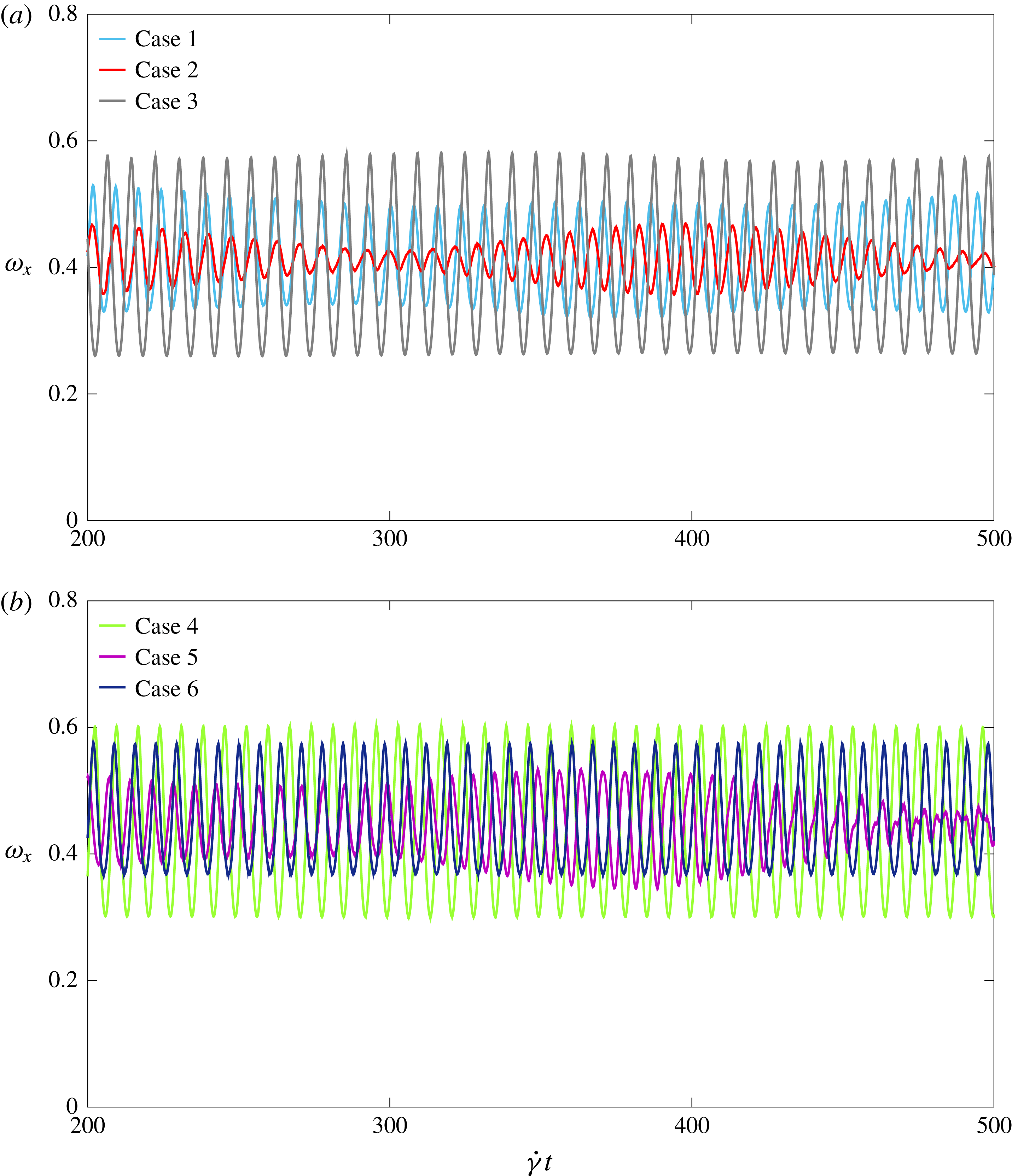
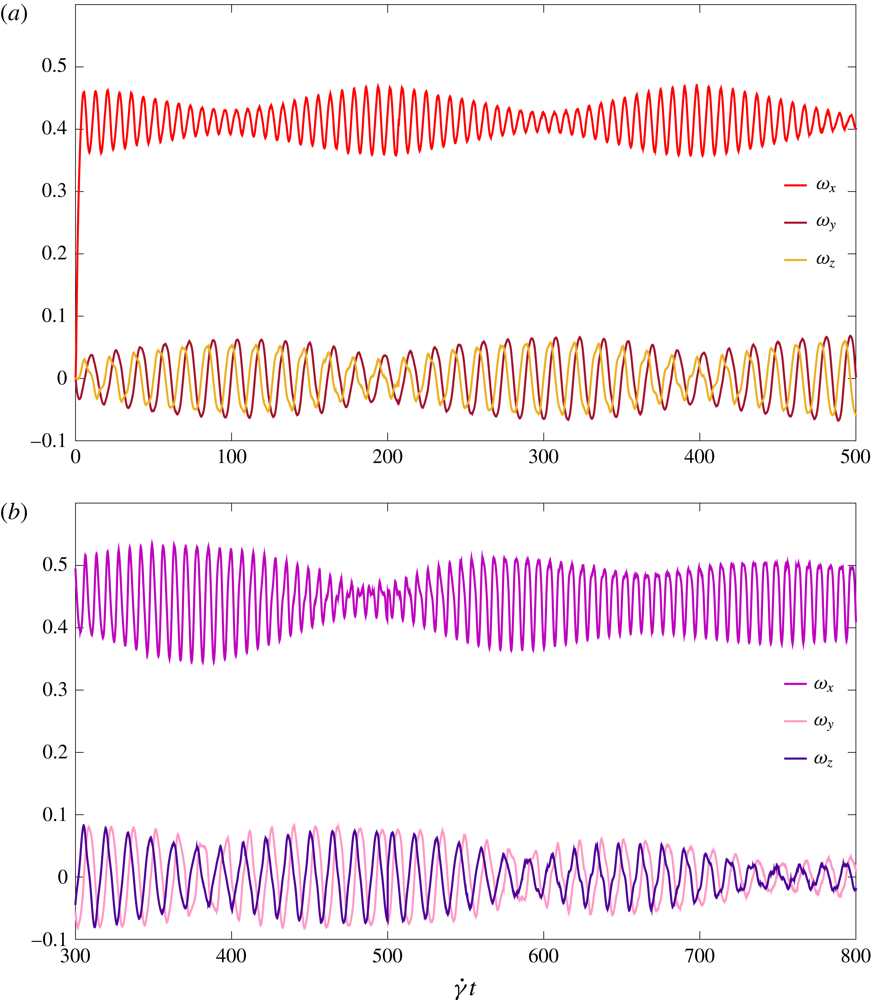
Angular velocity about the vorticity vector in a shear field is shown as a function of dimensionless time for two irregular-shaped particles (a)
 $\beth$
and (b)
 $\aleph$
for three different initial orientations. Angular velocity in all cases varies from one cycle to another but its cycle-averaged values become almost constant after the first rotation.

3.1 Instantaneous kinematics and final state of rotational motion
The background shear flow exerts a hydrodynamic torque on the particle which creates a tumbling motion mainly around the vorticity direction of the background flow (
 $x$
-direction). Therefore, the angular velocity around this direction
 $\unicode[STIX]{x1D714}_{x}$
is plotted as a function of time in figure 4, which shows an oscillatory behaviour for all cases. Maximums and minimums of
 $\unicode[STIX]{x1D714}_{x}$
are associated with maximums and minimums of the projected area against the flow, respectively. Similar to the rotation of a spheroid, a complete rotation (cycle) about the vorticity direction consists of four peaks (two maximums and two minimums) (Mueller et al.
Reference Mueller, Llewellin and Mader2010; Daghooghi & Borazjani Reference Daghooghi and Borazjani2015b
).
 $\unicode[STIX]{x1D714}_{x}$
is the major component of angular velocity with a non-zero (proportional to the shear rate) cycle-averaged value. The amplitudes of the other components (
 $\unicode[STIX]{x1D714}_{y}$
and
 $\unicode[STIX]{x1D714}_{z}$
) are considerably smaller than
 $\unicode[STIX]{x1D714}_{x}$
for all cases, and oscillate around zero. These characteristics of angular velocity are in qualitative agreement with the kayaking motion (both precession and nutation around the vorticity direction) of any axisymmetric particle (Jeffery Reference Jeffery1922; Bretherton Reference Bretherton1962; Huang et al.
Reference Huang, Yang, Krafczyk and Lu2012b
). The term ‘kayaking’ is borrowed from the prolate spheroid, where the same type of rotation resembles the motion of a kayak paddle (Rosén et al.
Reference Rosén, Do-Quang, Aidun and Lundell2015b
). Figure 5 compares all components of angular velocity in case 2 and case 5. In case 3, case 4 and case 6,
 $\unicode[STIX]{x1D714}_{y}$
and
 $\unicode[STIX]{x1D714}_{z}$
are almost negligible (planar motion), and in case 1, the amplitudes of
 $\unicode[STIX]{x1D714}_{y}$
and
 $\unicode[STIX]{x1D714}_{z}$
are comparable to case 2 and case 5. The motion of the particle
 $\beth$
(kayaking versus planar) for cases 1 to 3 can be better observed in supplementary movie 1 available at https://doi.org/10.1017/jfm.2018.65.
Three components of the angular velocity vector are compared for two cases which have the highest ratio of
 $\unicode[STIX]{x1D714}_{y}$
and
 $\unicode[STIX]{x1D714}_{z}$
with respect to
 $\unicode[STIX]{x1D714}_{x}$
for each particle: (a)
 $\beth$
and (b)
 $\aleph$
. The amplitude of
 $\unicode[STIX]{x1D714}_{y}$
and
 $\unicode[STIX]{x1D714}_{z}$
are considerably smaller than
 $\unicode[STIX]{x1D714}_{x}$
, and oscillate around zero. The characteristics of angular velocity are in qualitative agreement with the kayaking motion (both precession and nutation around the vorticity direction) of any axisymmetric particle.

For a spheroid in the absence of inertia, the kayaking motion (the limiting cases are log-rolling and tumbling) is periodic and the trajectory of the particle’s axis is a closed curve (Jeffery’s orbit). Consequently, maximums and minimums of angular velocity remain unchanged. These extremums are functions of the orbit constant
 $C$
and, based on our simulations for prolate spheroids (not shown here), the amplitude of oscillations for
 $\unicode[STIX]{x1D714}_{x}$
increases with
 $C$
, while the cycle-averaged values remain constant. With added fluid inertia, the symmetry in the Stokes flow around the particle is disturbed (Rosén et al.
Reference Rosén, Lundell and Aidun2014) and the degeneracy of this periodic motion will break (Rosén et al.
Reference Rosén, Do-Quang, Aidun and Lundell2015b
). Breaking the periodicity of angular motion could also happen even in Stokes flow for non-axisymmetric particles (Hinch & Leal Reference Hinch and Leal1979; Yarin et al.
Reference Yarin, Gottlieb and Roisman1997). In either case, the motion of particles during their rotation is not steady and the amplitude of oscillation can vary from one cycle to another, i.e., drift from one orbit to another. In our simulations, both factors (inertia and non-axisymmetric shape) are present and significant cycle-to-cycle variations can be clearly seen for case 1, case 2, and case 5 in figures 4 and 5, while cyclic variations are small in the other cases. Figure 5 shows that during the cyclic variation, when the amplitude of
 $\unicode[STIX]{x1D714}_{x}$
decreases, the amplitude of angular velocity in the other directions (
 $\unicode[STIX]{x1D714}_{y}$
and
 $\unicode[STIX]{x1D714}_{z}$
) increases, and vice versa. This is also in agreement with our simulations for spheroids (not shown here) when rotating in different orbits.
In addition to the cyclic variations shown in figures 4 and 5, discrete Fourier transform (DFT) analysis of
 $\unicode[STIX]{x1D714}_{x}$
confirms multiple dominant frequencies in the angular velocity oscillations. Multiple dominant frequencies of oscillation in angular velocity have been reported in the motion of a triaxial ellipsoid (Hinch & Leal Reference Hinch and Leal1979; Yarin et al.
Reference Yarin, Gottlieb and Roisman1997) or a spheroid when inertial effects are significant (Huang et al.
Reference Huang, Wu and Lu2012a
). The most dominant frequency
 $\mathfrak{f}$
in each case (shown in table 2) can be considered as a rotation in a Jeffery’s orbit and other frequencies can be seen as the drift of a particle from one orbit to another, probably due the non-axisymmetric shape and also inertial effects. In other words, cycle-to-cycle variations of angular velocity in figures 4 and 5 resemble the orbit drift phenomenon in spheroids. The rate of the cyclic variations (orbit drift) is different for different cases, and depends on the particle’s shape and its initial orientation, which is consistent with recent numerical simulations of spheroids subjected to inertia (Yu et al.
Reference Yu, Phan-Thien and Tanner2007; Mao & Alexeev Reference Mao and Alexeev2014; Rosén et al.
Reference Rosén, Lundell and Aidun2014).
A considerable amount of numerical and theoretical work has been recently devoted to determine the final state of rotational motion for axisymmetric particles with fluid and particle inertia (see Dabade et al. (Reference Dabade, Marath and Subramanian2016) for a recent review). For very weak fluid inertia (
 $Re\ll 1.0$
), analytical analyses show that spheroids drift towards a preferred orbit (either tumbling or log-rolling) depending on the type of spheroid (oblate versus prolate) and the aspect ratio, regardless of the initial orientation (Subramanian & Koch Reference Subramanian and Koch2005, Reference Subramanian and Koch2006; Dabade et al.
Reference Dabade, Marath and Subramanian2016). Even at similar Reynolds numbers to ours (
 $Re\approx 1$
), spheroids with different initial orientations are expected to converge into a unique final state of rotation (tumbling or log-rolling) (Rosén et al.
Reference Rosén, Lundell and Aidun2014, Reference Rosén, Do-Quang, Aidun and Lundell2015a
,Reference Rosén, Do-Quang, Aidun and Lundell
b
,Reference Rosén, Einarsson, Nordmark, Aidun, Lundell and Mehlig
c
). Nevertheless, our results for angular velocity do not show such a migration towards a preferred orbit of rotation. In fact, our results in figures 4 and 5 clearly show that, depending on the initial orientation, particles can maintain their initial state of rotation for a relatively long period of time (see case 4 and case 6). Other cases that have larger cycle-to-cycle variations do not show any sign of convergence towards a preferred motion (see case 1 and case 2). Dependence of state of rotation on the initial orientation under the presence of inertia is in agreement with the recent numerical simulations for spheroids at sufficiently high
 $Re$
(Yu et al.
Reference Yu, Phan-Thien and Tanner2007; Rosén et al.
Reference Rosén, Lundell and Aidun2014, Reference Rosén, Do-Quang, Aidun and Lundell2015a
,Reference Rosén, Do-Quang, Aidun and Lundell
b
,Reference Rosén, Einarsson, Nordmark, Aidun, Lundell and Mehlig
c
). Yu et al. (Reference Yu, Phan-Thien and Tanner2007) and Rosén et al. (Reference Rosén, Lundell and Aidun2014, Reference Rosén, Do-Quang, Aidun and Lundell2015a
,Reference Rosén, Do-Quang, Aidun and Lundell
b
,Reference Rosén, Einarsson, Nordmark, Aidun, Lundell and Mehlig
c
) noticed a bifurcation phenomena in the orbital motion of spheroids, i.e., orbit behaviour is sensitive to the initial orientation and there exist different equilibrium (final) rotational states for certain shear Reynolds number regimes. To explain this complex behaviour, Rosén et al. (Reference Rosén, Do-Quang, Aidun and Lundell2015a
) mentioned the importance of particle inertial effects for neutrally buoyant particles as a missing point in some numerical simulations. They hypothesize that if the particle is released at an orientation where the symmetry axis gains enough angular momentum, centrifugal forces will take it to a planar tumbling motion (e.g. case 4 and case 6) (Rosén et al.
Reference Rosén, Lundell and Aidun2014, Reference Rosén, Do-Quang, Aidun and Lundell2015a
). Otherwise, fluid inertia effects will dominate, leading to a non-planar motion such as kayaking motion (case 2 and case 5) (Rosén et al.
Reference Rosén, Lundell and Aidun2014, Reference Rosén, Do-Quang, Aidun and Lundell2015a
).
Another influential factor affecting orbit change and the final state of rotation is the geometry (shape) of the particles. All the aforementioned numerical studies (Yu et al.
Reference Yu, Phan-Thien and Tanner2007; Huang et al.
Reference Huang, Wu and Lu2012a
,Reference Huang, Yang, Krafczyk and Lu
b
; Mao & Alexeev Reference Mao and Alexeev2014; Rosén et al.
Reference Rosén, Lundell and Aidun2014, Reference Rosén, Do-Quang, Aidun and Lundell2015a
,Reference Rosén, Do-Quang, Aidun and Lundell
b
,Reference Rosén, Einarsson, Nordmark, Aidun, Lundell and Mehlig
c
) observed a rich rotational behaviour for oblate or prolate spheroids with a limited range of aspect ratio (
 $2\leqslant r_{e}\leqslant 5$
), and it was envisioned that the complexity of rotational dynamics increases for low-aspect-ratio spheroids when
 $r_{e}<2$
(Rosén et al.
Reference Rosén, Do-Quang, Aidun and Lundell2015a
) or the axisymmetry breaks (Lundell Reference Lundell2011), which is in agreement with our results shown in figures 4 and 5. Contrary to spheroids, a final state of rotation cannot be seen for all cases even after a considerable amount of time (e.g. more than 70 cycles of rotation for case 5). In case 2, motion of the particle is close to a doubly periodic motion, which is analogous to a near-axisymmetric triaxial ellipsoid (Hinch & Leal Reference Hinch and Leal1979). This doubly periodic motion can be better seen in figures 5(a) for all components of angular velocity. Hinch & Leal (Reference Hinch and Leal1979) showed that, in the absence of inertia, near-axisymmetric ellipsoids could have a doubly periodic motion; a relatively rapid rotation which corresponds to the motion of axisymmetric particle around Jeffrey orbits, and a slower drift as a periodic change in the orbit if particles were axisymmetric (Hinch & Leal Reference Hinch and Leal1979). It should be noted that the motion of particle
 $\beth$
in case 2 is not precisely doubly periodic and has other (relatively slower) modes based on DFT, which can be due to inertial effects or complexity of shape. Case 1 and especially case 5 have more complex and unstable motions and show unpredictable drift motion within the simulation time span. This unstable rotational motion that may turn into a chaotic behaviour has also been observed in triaxial ellipsoids for sufficiently high aspect ratios (Yarin et al.
Reference Yarin, Gottlieb and Roisman1997). Figures 4(b) and 5(b) together clearly show the unstable rotational motion of particle
 $\aleph$
(case 5) in a relatively wide time span.
3.2 Equivalent spheroids based on kinematics of motion
As an essential step towards discussing the role of geometry on the particle stress, we need to obtain equivalent spheroids for irregular particles, against which they are compared. These regular equivalents are found based on the motion of the irregular particles as discussed in § 2.4.
Based on (2.6), the effective aspect ratio of the equivalent spheroid is a function of the period of rotation. We calculated the period of rotation for each case in two ways to ensure the accuracy of calculations: (1) using the most dominant frequency in DFT analysis of the angular velocity (
 $t_{r}=2/\mathfrak{f}$
); and (2) calculating the swept angle.
Since the main rotation occurs around the vorticity vector, the rotation of the particle projected in the shear plane (denoted by
 $\unicode[STIX]{x1D703}$
) is considered to calculate the cyclic rotation of particles. The swept angle in the shear plane is calculated as the following:
 $$\begin{eqnarray}\unicode[STIX]{x1D703}(t)=\int _{0}^{t}\unicode[STIX]{x1D714}_{x}\,\text{d}\unicode[STIX]{x1D70F},\end{eqnarray}$$
where
 $\unicode[STIX]{x1D714}_{x}$
is the component of the particle’s angular velocity along the vorticity vector of the flow. We considered several rotation cycles (30 cycles) and obtained the period of rotation based on the average value of the cycles.
The time periods of rotation
 $t_{r}$
from both methods are compared and found to be within 1 % of each other. Results for the time period
 $t_{r}$
, the effective aspect ratio
 $r_{e}$
, and the average angular velocity
 $\bar{\unicode[STIX]{x1D714}}_{x}$
for all six simulated cases are shown in table 2. Note that, for each case,
 $r_{e}>1$
represents equivalent prolates while
 $r_{e}<1$
(values in the parentheses) corresponds to equivalent oblates. The range of effective aspect ratio based on kinematics for all cases (
 $1.5<r_{e}\leqslant 2.0$
) is in good agreement with the approximate geometric aspect ratios for these particles. Therefore, for the rest of the paper, we do not distinguish between equivalent spheroids obtained based on the geometry or the kinematics.
Our results clearly show that the time period of rotation, average angular velocity, and effective aspect ratio for all cases of each particle are close, and initial orientation does not affect these kinematic parameters by more than 8 %. This is in agreement with analytical solutions of Jeffery (Reference Jeffery1922) for spheroids and Bretherton (Reference Bretherton1962) for general axisymmetric particles, which indicate that the time period of rotation (
 $t_{r}$
) is independent of initial orientation and only depends on aspect ratio – see the time period of rotation in table 2. It should also be noted that the average angular velocities for all cases are slightly lower than 0.5, i.e., close to the analytical solution for spheres and spheroids. The lower angular velocity in our results is due to the influence of inertia, which has been reported for various shapes of particles in numerical (Aidun et al.
Reference Aidun, Lu and Ding1998; Mikulencak & Morris Reference Mikulencak and Morris2004; Daghooghi & Borazjani Reference Daghooghi and Borazjani2015b
), and experimental studies (Robertson & Acrivos Reference Robertson and Acrivos1970).
4 Shear particle stress and intrinsic viscosity
The prime aim of this study is to investigate the role of particle geometry on the rheological properties and particle stress and evaluate the accuracy of approximating an irregular-shaped particle with equivalent regular shapes such as spheroids or spheres. Viscometric functions of a suspension
 $(\unicode[STIX]{x1D702}_{r},N_{1},N_{2})$
, are functions of the volume-averaged particle stress tensor (2.5). Therefore, we seek to know how the geometry of suspended particles may influence the particle stress.
4.1 Shear particle stress
The most dominant part of shear particle stress is the stresslet
 $\unicode[STIX]{x1D61A}_{yz}$
(2.3) and our calculations show that the averaged values of acceleration stress
 $\unicode[STIX]{x1D617}_{yz}$
and Reynolds stress
 $\unicode[STIX]{x1D619}_{yz}$
are negligible compared to the stresslet
 $\unicode[STIX]{x1D61A}_{yz}$
contribution at
 $Re=1.0$
. In fact, the average Reynolds stress and acceleration stress are almost zero and their root mean square values are two orders of magnitude smaller than that of the stresslet, similar to what was found in our previous work for spheroids (Daghooghi & Borazjani Reference Daghooghi and Borazjani2015b
). Moreover, shear acceleration stress and shear Reynolds stress are out of phase and cancel each other out, giving a negligible contribution to the total particle stress, similar to spheroidal particles (Daghooghi & Borazjani Reference Daghooghi and Borazjani2015b
).
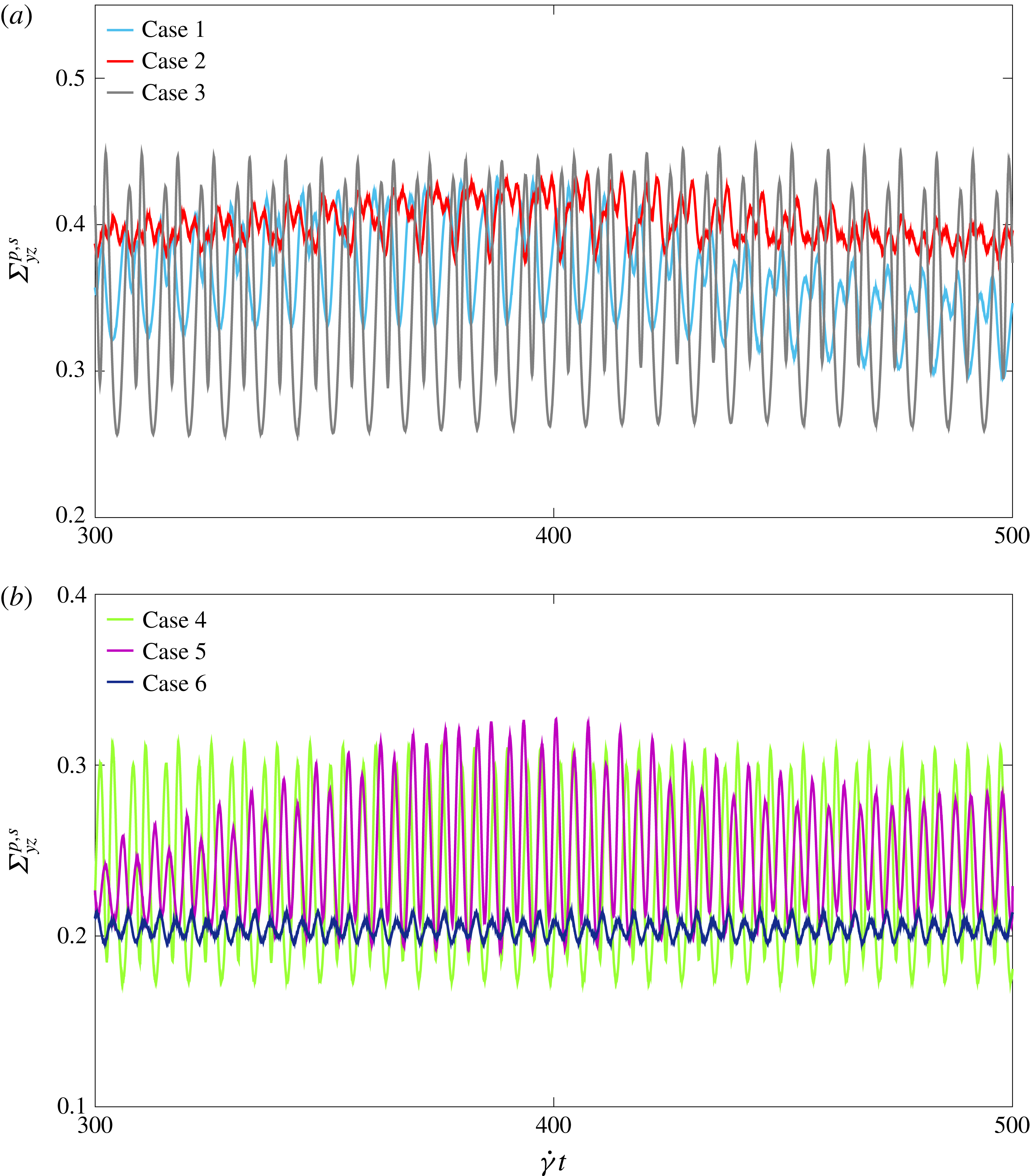
Instantaneous shear particle stress is shown as a function of time for two complex-shaped particles (a)
 $\beth$
and (b)
 $\aleph$
with different initial orientations. The time (angle) history of particle stress is more complicated compared to angular velocity, as it is a nonlinear function of the particle’s shape and kinematics.

Figure 6 shows the instantaneous shear particle stress
 $\unicode[STIX]{x1D6F4}_{yz}^{p}$
during the rotation of a particle for all cases. As expected and mentioned in § 1, in the absence of non-hydrodynamic forces, the particle stress of a given particle (given shape) is a function of its orientation, which is a function of time. However, our results show that in the presence of inertia the particle stress of an irregular-shaped particle is not precisely a simple periodic function of time, and other frequencies are involved, as discussed in § 3.1. The frequencies of oscillation for shear particle stress
 $\unicode[STIX]{x1D6F4}_{yz}^{p}$
are very close to the corresponding ones for angular velocity
 $\unicode[STIX]{x1D714}_{x}$
. Nevertheless, its time history is more complicated compared to angular velocity, since particle stress depends nonlinearly on a particle’s shape and orientation. For instance, this can be easily seen by comparing angular velocity and shear stress for case 4 and case 6, where a small difference in angular velocity between two cases results in a significantly higher amplitude of shear stresslet, or in case 1, where small cycle-to-cycle variations in
 $\unicode[STIX]{x1D714}_{x}$
(due to orbital change) cause relatively larger variations in
 $\unicode[STIX]{x1D6F4}_{yz}^{p,s}$
. In addition, comparison of figures 5 and 6 also shows that the amplitudes of
 $\unicode[STIX]{x1D714}_{x}$
and
 $\unicode[STIX]{x1D6F4}_{yz}^{p,s}$
increase or decrease in phase, whereas
 $\unicode[STIX]{x1D714}_{y}$
and
 $\unicode[STIX]{x1D714}_{z}$
are in opposite phase to the shear particle stress. This suggests that the shear stresslet is more sensitive to
 $\unicode[STIX]{x1D714}_{x}$
than the two other components of the angular velocity vector.
It should be noted that the motion of particles is not the main parameter affecting the stresslet behaviour because the motion itself depends on other parameters such as the particle’s shape and inertia. Comparing the shear particle stress
 $\unicode[STIX]{x1D6F4}_{yz}^{p,s}$
of both particles in figure 6, one can easily observe that the slender particle
 $\beth$
(cases 1 to 3) produces a higher value of stress than particle
 $\aleph$
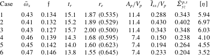
(cases 4 to 6). The average shear particle stress (stresslet) for all cases is calculated and shown in table 2. As can be clearly seen in the table, both particles
 $\aleph$
and
 $\beth$
have close effective aspect ratios, time periods, average angular velocities, whereas the particle stress of particle
 $\beth$
is significantly (approximately 50 %) higher than particle
 $\aleph$
. This difference may seem surprising, as particle
 $\beth$
is expected to experience a lower resistance force (see the slender shape and holes on it in figure 1) compared to particle
 $\aleph$
.
To explain this qualitative contradiction, the following approximate equation for particle stress is helpful (acceleration and Reynolds stress terms are negligible):
 $$\begin{eqnarray}\unicode[STIX]{x1D6F4}_{yz}^{p}\approx \unicode[STIX]{x1D719}\frac{\unicode[STIX]{x1D61A}_{yz}}{V_{p}},\end{eqnarray}$$
where
 $\unicode[STIX]{x1D719}$
is the suspension’s volume fraction and only one particle in the computational domain is considered. As can be seen in (4.1), at an equal volume fraction, particle stress is proportional to stresslet per unit volume of a particle. Stresslet, as defined in (2.4a
), is the surface integral of the moment of stress with respect to its centre of mass.
To investigate the shear stress (non-dimensionalized by
 $\unicode[STIX]{x1D70C}\dot{\unicode[STIX]{x1D6FE}}^{2}\mathfrak{L}^{2}$
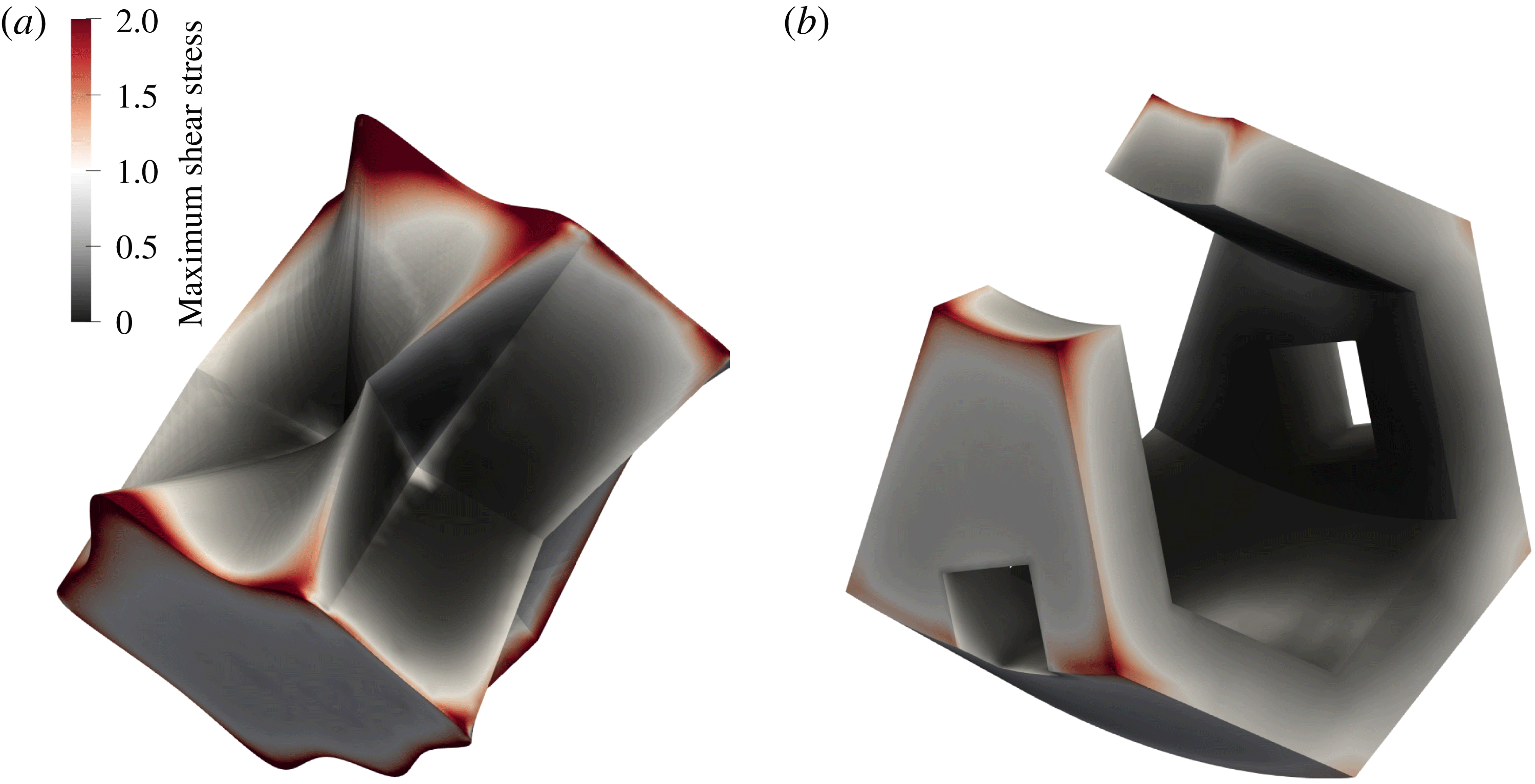
) distribution on the particle, the cycle-averaged maximum stress projected onto the surface of particles for case 2 (particle
 $\beth$
) and case 6 (particle
 $\aleph$
) are visualized and compared in figure 7. To obtain the maximum stress, the principal stress of the shear stress tensor
 $\unicode[STIX]{x1D749}$
is first calculated by solving the following equation:
 $$\begin{eqnarray}\unicode[STIX]{x1D706}^{3}-I_{1}\unicode[STIX]{x1D706}^{2}+I_{2}\unicode[STIX]{x1D706}-I_{3}=0,\end{eqnarray}$$
where
 $I_{1}=\text{tr}(\unicode[STIX]{x1D749})$
,
 $I_{2}=0.5(\text{tr}(\unicode[STIX]{x1D749}^{2})-\text{tr}(\unicode[STIX]{x1D749})^{2})$
, and
 $I_{3}=\text{det}(\unicode[STIX]{x1D749})$
are the first, second, and third invariants of the stress tensor and
 $\text{tr}(\unicode[STIX]{x1D749})$
and
 $\text{det}(\unicode[STIX]{x1D749})$
denote trace and determinant of the shear stress tensor
 $\unicode[STIX]{x1D749}$
, respectively (Panton Reference Panton1996). The maximum principal shear stress
 $\unicode[STIX]{x1D749}_{max}$
is the maximum root of (4.2). Values of
 $\unicode[STIX]{x1D749}_{max}$
computed on the fluid grid nodes closest to the particle are then projected onto the particle surface. Finally, this maximum shear stress is averaged during one cycle of rotation. The shear stress of the bulk flow is equal to
 $\unicode[STIX]{x1D70F}_{yz}=1.0$
(coloured as white), with dark grey and red indicating the lowest and highest amount of shear stress on the surface of a particle, respectively. Comparing particles
 $\beth$
and
 $\aleph$
in this figure clearly shows that the values of surface stress on both particles are qualitatively similar (highest and lowest values of the stress mostly occur at external and internal corners and edges, respectively) and ranges within a similar interval, i.e., the shear stress on the surface of both particles has the same order of magnitude. Consequently, at equal particle volume
 $V_{p}$
, a similar resistance force (stress) on the surface of particle
 $\beth$
(which has a curved slender geometry) is integrated over a higher surface area, compared to particle
 $\aleph$
, which makes this surface integral higher. In fact, our calculation shows that the dimensionless surface-to-volume ratio of particle
 $\beth$
is 11.4, whereas this ratio for particle
 $\aleph$
is only 7.4, i.e.
 $A_{p}/V_{p}$
of particle
 $\beth$
is approximately 50 % higher than particle
 $\aleph$
. This is almost the same ratio by which particle
 $\beth$
experiences higher shear particle stress. In other words, the dimensionless surface-to-volume ratio
 $A_{p}/V_{p}$
(both
 $A_{p}$
and
 $V_{p}$
are non-dimensionalized by the one-half the largest diameter of the particle
 $\mathfrak{L}$
) can help in comparing the average particle stress of different geometries (considering all orbits of rotations). However, this parameter cannot show the effect of a particle’s orientation on shear stress.
The cycle-averaged maximum shear stress for (a) case 2 (particle
 $\beth$
) and (b) case 6 (particle
 $\aleph$
). The shear stress of the bulk flow is equal to
 $\unicode[STIX]{x1D70F}_{yz}=1.0$
(coloured as white) and dark grey and red indicate lowest and highest amount of shear stress on the surface of a particle, respectively.

Another important geometric criterion which can be used to predict shear particle stress is the moment of inertia with respect to the vorticity direction per unit particle volume
 $I_{xx}/V_{p}$
(non-dimensionalized by
 $\unicode[STIX]{x1D70C}\mathfrak{L}^{2}$
). Note that
 $I_{xx}$
changes based on the orientation of the particle relative to the
 $x$
-axis. Considering the definition of shear stresslet (2.4a
), a longer distance of the surface with respect to the vorticity axis under a similar stress distribution (figure 7) results in a higher value of the integrand function and, consequently, a higher value of shear particle stress
 $\unicode[STIX]{x1D6F4}_{yz}^{p,s}$
at equal volume fractions
 $\unicode[STIX]{x1D719}$
. Among different cases for each particle in table 2, averaged results in the table also show that the
 $I_{xx}/V_{p}$
factor correlates with the shear particle stress – i.e., the higher value of
 $I_{xx}/V_{p}$
, the higher particle stress.
Considering particle shape and initial orientation, therefore, we can conclude that particles with higher slenderness ratio (
 $A_{p}/V_{p}$
) and with a mass distribution further from the centre of mass around the vorticity direction (
 $I_{xx}/V_{p}$
) generate more stresslet at constant volume fraction, and the viscosity of a suspension is consequently higher. These geometric parameters are consistent with the results obtained for regular geometries such as spheroids – i.e., spheroids with higher aspect ratio have higher
 $A_{p}/V_{p}$
and
 $I_{xx}/V_{p}$
, and also a higher shear stresslet (Jeffery Reference Jeffery1922; Daghooghi & Borazjani Reference Daghooghi and Borazjani2015b
).
4.1.1 Mathematically defined particles
To further test the effects of the two geometric factors (
 $A_{p}/V_{p}$
and
 $I_{xx}/V_{p}$
), we performed simulations on two families of mathematically defined particles: a family of cylinders and a family of sphere-like particles at a similar volume fraction and Reynolds number, with other cases consisting of particles
 $\aleph$
and
 $\beth$
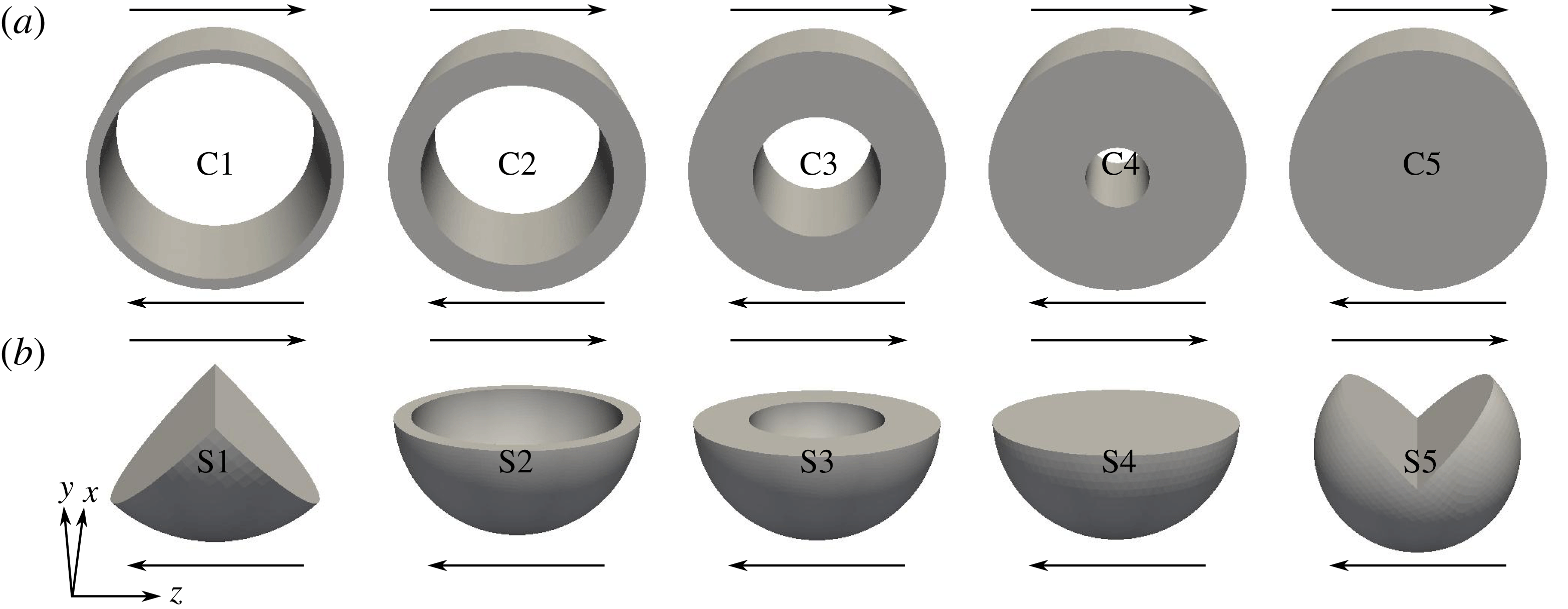
. Figure 8 shows the 3-D schematic of both families and their orientation with respect to the shear flow. The family of cylinders in figure 8(a) have equal outer diameter
 $D=2.0$
and length
 $L=1.0$
, while the inner diameter is
 $(0.9,0.75,0.5,0.25)$
for (C1, C2, C3, C4), respectively. The family of spheres in figure 8(b) consists of a quarter sphere (S1), two hollow hemispheres S2 and S3, a solid hemisphere S4, and a three-quarter sphere S5. The outer radius of all sphere-like particles is equal to
 $R=1.0$
and the inner radius is
 $(0.86,0.577)$
for (S2, S3), respectively. It can be easily seen that all these particles have aspect ratios and diameters close to particles
 $\aleph$
and
 $\beth$
.
3-D schematic of two families of mathematically defined particles to test our hypothesis about the geometric effective factors (surface-to-volume ratio and moment of inertia per unit volume) on the shear particle stress. (a) Family of cylinders with equal outer diameter
 $D=2.0$
and length
 $L=1.0$
. (b) Family of sphere-like particles with radius
 $R=1.0$
. The solid arrows show the direction of shear flow around the particle.

Surface-to-volume ratio
 $A_{p}/V_{p}$
, moment of inertia along the vorticity vector per unit particle volume
 $\bar{I}_{xx}/V_{p}$
and averaged shear particle stress
 $\bar{\unicode[STIX]{x1D6F4}}_{yz}^{p,s}$
.

The surface-to-volume ratio
 $A_{p}/V_{p}$
, the moment of inertia per unit volume
 $I_{xx}/V_{p}$
and the averaged particle stress
 $\bar{\unicode[STIX]{x1D6F4}}_{yz}^{p,s}$
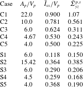
are calculated and shown in table 1. For the cylinder particles, particle stress decreases monotonically as both geometric parameters decrease from C1 to C5. In fact, the particle stress
 $\bar{\unicode[STIX]{x1D6F4}}_{yz}^{p,s}$
varies almost linearly with the surface-to-volume ratio. In particular, the hollow cylinder C1 has a high surface-to-volume ratio of
 $A_{p}/V_{p}=22.0$
and also a high value of
 $I_{xx}/V_{p}=0.90$
, both of which are approximately two times those of case 2 (highest values of geometric factors). Accordingly, the shear particle stress at equal
 $Re$
and
 $\unicode[STIX]{x1D719}$
for this case is
 $\bar{\unicode[STIX]{x1D6F4}}_{yz}^{p,s}=1.07$
, which is approximately 2.6 times that of case 2, which has the highest
 $\bar{\unicode[STIX]{x1D6F4}}_{yz}^{p,s}$
among the irregular particles. The role of geometric parameters on the particle stress can also be verified in the family of sphere-like particles. Comparing cases S1 and S3, which have equal values of surface-to-volume ratio, the particle stress of S3 with a higher value of
 $I_{xx}/V_{p}$
is also higher than particle S1. In the same way, cases S2 and S5 have similar values of
 $I_{xx}/V_{p}$
, and the particle stress of S2 with higher
 $A_{p}/V_{p}$
is also higher than S5. Additionally, considering cases S2, S3 and S4, the particle stress decreases monotonically when both geometric parameters decrease, similar to the cylinder family.
The importance of these geometric factors on the shear particle stress can be better understood when one considers a geometric equivalent for an irregular-shaped particle. For instance,
 $\bar{\unicode[STIX]{x1D6F4}}_{yz}^{p,s}$
of the hollow cylinder C1, which has a geometric aspect ratio
 $D/L=2.0$
, is approximately six times that of a prolate spheroid (
 $r_{e}=2.0$
) at the same
 $Re$
and
 $\unicode[STIX]{x1D719}$
(Daghooghi & Borazjani Reference Daghooghi and Borazjani2015b
), or more than five times that of an oblate spheroid (
 $r_{e}=0.5$
) assuming Stokes flow (Jeffery Reference Jeffery1922).
4.2 Consequences for intrinsic viscosity
One important consequence of the role of geometry on the shear particle stress is the effect on the intrinsic viscosity of a suspension. In low volume fractions, the relative viscosity as a function of volume fraction can be approximated as
 $\unicode[STIX]{x1D702}_{r}=1+[\unicode[STIX]{x1D702}]\unicode[STIX]{x1D719}+k_{H}\unicode[STIX]{x1D719}^{2}$
, where
 $[\unicode[STIX]{x1D702}]$
and
 $k_{H}$
are the intrinsic viscosity and Huggins coefficient, respectively. The second-order term
 $k_{H}\unicode[STIX]{x1D719}^{2}$
is considered when particle interactions need to be included in the calculation, whereas in dilute regimes the intrinsic viscosity
 $[\unicode[STIX]{x1D702}]$
causes the primary effect of a particle’s shape on the relative viscosity. Since our simulations are in the dilute regime, we ignore the second-order term to calculate the intrinsic viscosity
 $[\unicode[STIX]{x1D702}]$
by:
 $$\begin{eqnarray}[\unicode[STIX]{x1D702}]=Re\bar{\unicode[STIX]{x1D6F4}}_{yz}^{p,s}/\unicode[STIX]{x1D719}\end{eqnarray}$$
based on the previously calculated averaged shear particle stress.
 $[\unicode[STIX]{x1D702}]$
values calculated for our cases are tabulated in table 2. Note that this is not the
 $[\unicode[STIX]{x1D702}]$
of an actual suspension of particles in many orbits, but a periodic suspension with a given orbit (Huang et al.
Reference Huang, Wu and Lu2012a
; Rosén et al.
Reference Rosén, Do-Quang, Aidun and Lundell2015a
,Reference Rosén, Do-Quang, Aidun and Lundell
b
,Reference Rosén, Einarsson, Nordmark, Aidun, Lundell and Mehlig
c
). This assumption will be discussed further at the end of this section.
Averaged angular velocity
 $\bar{\unicode[STIX]{x1D714}}_{x}$
, most dominant frequency in angular velocity oscillations
 $\mathfrak{f}$
, period of rotation
 $t_{r}$
, effective aspect ratio
 $r_{e}$
(values inside parenthesis pertain to oblate spheroids), surface-to-volume ratio
 $A_{p}/V_{p}$
, averaged moment of inertia along the vorticity vector per unit particle volume
 $\bar{I}_{xx}/V_{p}$
, averaged shear particle stress
 $\bar{\unicode[STIX]{x1D6F4}}_{yz}^{p,s}$
and intrinsic viscosity
 $[\unicode[STIX]{x1D702}]$
of the suspension.

In order to quantify the effect of a particle’s shape on the intrinsic viscosity, we compare this value with the intrinsic viscosity of their equivalent regular particles.
 $[\unicode[STIX]{x1D702}]$
for non-Brownian suspensions depends on the shape, size, and orientation of particles, and can be determined analytically (Stokesian solution) for simple shapes (Jeffery Reference Jeffery1922; Robertson & Acrivos Reference Robertson and Acrivos1970; Leal & Hinch Reference Leal and Hinch1971) and experimentally (Jeffrey & Acrivos Reference Jeffrey and Acrivos1976; Mueller et al.
Reference Mueller, Llewellin and Mader2010) for more general geometries and concentrations. In Stokes flows,
 $[\unicode[STIX]{x1D702}]$
for a sphere is calculated by Einstein (Reference Einstein1956) to be equal to 2.5, and for prolate and oblate spheroids is tabulated by Jeffery (Reference Jeffery1922) as a function of ellipticity. Jeffery calculated the time-averaged intrinsic coefficient by integrating the work that must be done to rotate a particle over a complete orbit (similar to our cycle-averaged calculation). However, this value depends on the initial orientation of a particle (orbit constant
 $C$
). Therefore, he tabulated the intrinsic viscosity for two limiting cases:
 $C=0$
(maximum value for oblate spheroids and minimum value for prolate spheroids); and
 $C\rightarrow \infty$
(minimum value for oblate spheroids and maximum value for prolate spheroids). To compare our results for
 $[\unicode[STIX]{x1D702}]$
with the corresponding value for a spheroid, we used the effective aspect ratio
 $r_{e}$
for each case (shown in table 2), and calculated upper and lower limits of intrinsic viscosity for spheroids (both oblate and prolate) with equal
 $r_{e}$
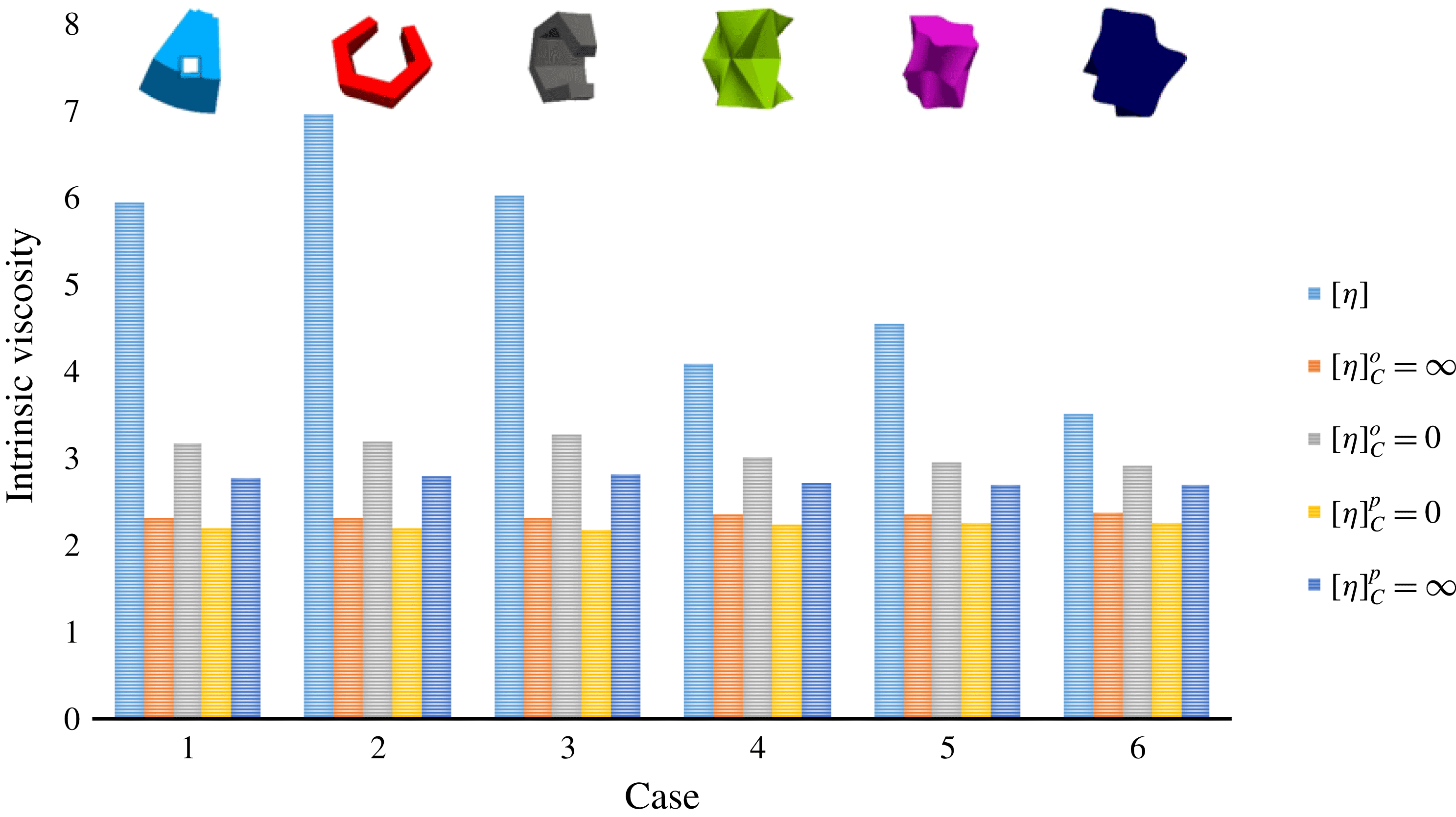
. Note that, comparing each case with its corresponding spheroid, both particles (an irregular particle and a spheroid) have an equal time period of rotation around the vorticity axis. Finding equivalent spheroids, we calculated limiting values for the intrinsic viscosity and compared with our cases in figure 9 as:
 $[\unicode[STIX]{x1D702}]_{C=0}^{o}$
, intrinsic viscosity for equivalent oblate spheroid at
 $C=0$
orbit;
 $[\unicode[STIX]{x1D702}]_{C=\infty }^{o}$
, intrinsic viscosity for equivalent oblate spheroid at
 $C=\infty$
orbit;
 $[\unicode[STIX]{x1D702}]_{C=0}^{p}$
, intrinsic viscosity for equivalent prolate spheroid at
 $C=0$
orbit; and
 $[\unicode[STIX]{x1D702}]_{C=\infty }^{p}$
, intrinsic viscosity for equivalent prolate spheroid at
 $C=\infty$
orbit.
The intrinsic viscosity
 $[\unicode[STIX]{x1D702}]$
of an irregular particle in comparison with that of equivalent oblate
 $[\unicode[STIX]{x1D702}]^{o}$
and prolate
 $[\unicode[STIX]{x1D702}]^{p}$
spheroids at
 $C=0$
and
 $C=\infty$
orbits. The intrinsic viscosities of suspensions for particle
 $\beth$
are approximately twice as large as equivalent spheroids for all the tested orientations.

A quick comparison between the computed
 $[\unicode[STIX]{x1D702}]$
for the original particles and similar values for equivalent spheroids in figure 9 or a sphere (
 $[\unicode[STIX]{x1D702}]=2.5$
) reveals that the irregular shape of a particle increases the intrinsic viscosity relative to equivalent simple geometries. In fact, the intrinsic viscosities of both particles are significantly higher than the maximum values of their equivalent spheroids for all the tested orientations. Note that the same argument is valid for particle stress, since at equal volume fraction and Reynolds number, intrinsic viscosity and shear particle stress are proportional according to (4.3). The greatest and the least difference can be seen in case 2 and case 4, in which the intrinsic viscosities (particle stress) are 20 % and 120 % higher than their equivalent oblate spheroids (oblate spheroids has a higher
 $[\unicode[STIX]{x1D702}]$
than prolate ones), respectively.
One may argue that this difference can be related to inertial effects, since inertia was found to cause an increase in the particle contribution to the viscosity of
 $O(Re)$
or
 $O(Re^{3/2})$
depending on the amount of inertia and volume fraction (Kulkarni & Morris Reference Kulkarni and Morris2008; Subramanian et al.
Reference Subramanian, Koch, Zhang and Yang2011; Yeo & Maxey Reference Yeo and Maxey2013). However, as Kulkarni & Morris (Reference Kulkarni and Morris2008) showed, this increase is not prominent at lower volume fractions, which is in agreement with our simulations for prolate spheroids in our previous publication (Daghooghi & Borazjani Reference Daghooghi and Borazjani2015b
), showing that inertia can only increase the particle stress (relative viscosity) slightly (less than 8 % for similar
 $\unicode[STIX]{x1D719}$
).
Another assumption in Jeffery’s solution is a dilute regime, which ignores particle interactions – i.e., equation (4.3) has an error of order
 $O(\unicode[STIX]{x1D719}^{2})$
. To investigate the influence of an
 $O(\unicode[STIX]{x1D719}^{2})$
error on the intrinsic viscosity
 $[\unicode[STIX]{x1D702}]$
, we repeated the simulation for case 6 with volume fraction
 $\unicode[STIX]{x1D719}=0.0086$
. It was found that, at such a low volume fraction, intrinsic viscosity could be approximately 10 % lower relative to simulations with
 $\unicode[STIX]{x1D719}=0.058$
– which is much lower than the difference between
 $[\unicode[STIX]{x1D702}]$
of irregular and spheroidal suspensions. We also ran another simulation with a sphere at a similar volume fraction and inertia, and found the intrinsic viscosity
 $[\unicode[STIX]{x1D702}]=2.77$
, which is 11 % higher than its Stokesian value in dilute suspensions. Additionally, in case 3 the equivalent spheroid has an effective aspect ratio
 $r_{e}=2.0$
, for which we have simulations of a prolate spheroid at exact
 $Re$
and
 $\unicode[STIX]{x1D719}$
(Daghooghi & Borazjani Reference Daghooghi and Borazjani2015b
). The maximum intrinsic viscosity for a prolate spheroid at (
 $Re=1.0,\unicode[STIX]{x1D719}=0.058$
) is
 $[\unicode[STIX]{x1D702}]_{C=\infty }^{p}=3.07$
(Daghooghi & Borazjani Reference Daghooghi and Borazjani2015b
), which is only 9 % higher than the Stokesian solution of Jeffery (Reference Jeffery1922), while particle
 $\beth$
in case 3 has 96 % higher intrinsic viscosity than the maximum value (
 $C=\infty$
) of its equivalent prolate spheroid at the same inertia and volume fraction. Therefore, the 20 %–120 % difference between investigated irregular-shaped particles and their equivalent regular particles is mainly due to the particle’s shape, and not the inertia or particle interactions
 $O(\unicode[STIX]{x1D719}^{2})$
. This difference increases with the slenderness of a particle; e.g., the intrinsic viscosity of the hollow cylinder C1 (figure 8) is more than seven times that of a sphere or five to six times that of a geometrically equivalent spheroid.
Note that in a real suspension, particles are located randomly and have different initial orientations. In the dilute limit, however, interaction of particles is negligible; hence, their individual contributions to viscosity can be averaged to determine the suspension viscosity (Mueller et al.
Reference Mueller, Llewellin and Mader2010). Accordingly,
 $[\unicode[STIX]{x1D702}]$
values in table 2 do not represent the intrinsic viscosity of a suspension but
 $[\unicode[STIX]{x1D702}]$
of a given orientation (orbit). Nevertheless, our results for all test cases show that shear particle stress and intrinsic viscosity are significantly higher than the maximum value of the equivalent spheroid. Therefore, we expect the combination of them, i.e., the intrinsic viscosity of a suspension with many particles in different orientations in the dilute regime, to have a value of
 $[\unicode[STIX]{x1D702}]$
higher than a suspension of equivalent spheroids.
5 Normal stress differences
In the limit of
 $Re\rightarrow 0$
, for pure hydrodynamic particle interactions (no Brownian motion and no direct particle contacts) with statistically symmetric microstructure, Stokes flow reversibility and symmetry of the imposed flow imply that normal stress differences are expected to be zero (Kumar & Higdon Reference Kumar and Higdon2011b
). However, when particles interact or when the inertia is not negligible, flow symmetry breaks down, which results in a net non-isotropic stress field (non-zero normal stress differences) within the suspension.
 $N_{1}$
and
 $N_{2}$
are generally functions of volume fraction, Reynolds number, particle’s shape, and particle’s orientation (Brenner Reference Brenner1974; Petrie Reference Petrie1999; Haddadi & Morris Reference Haddadi and Morris2014).
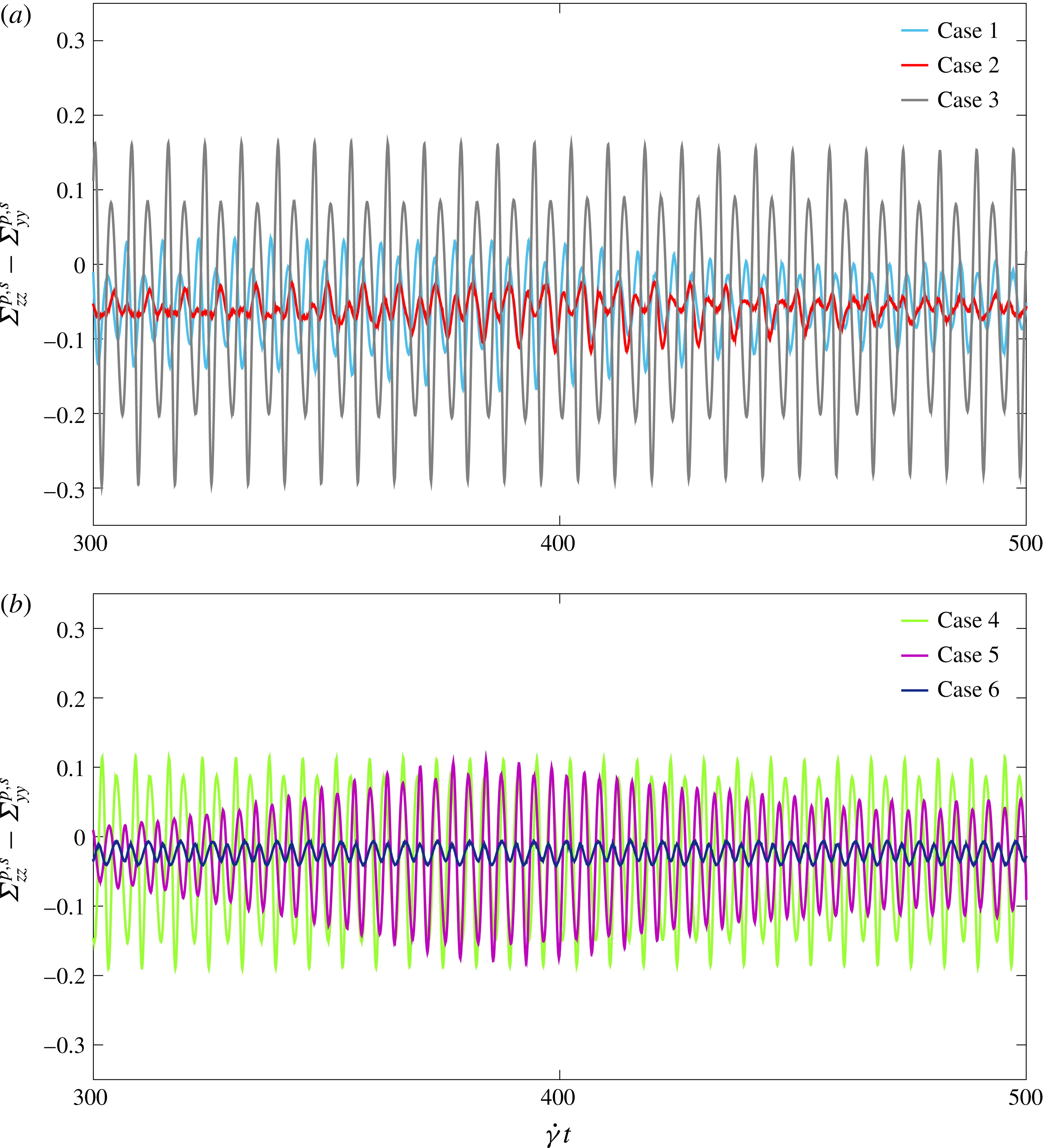
Instantaneous first normal stress difference
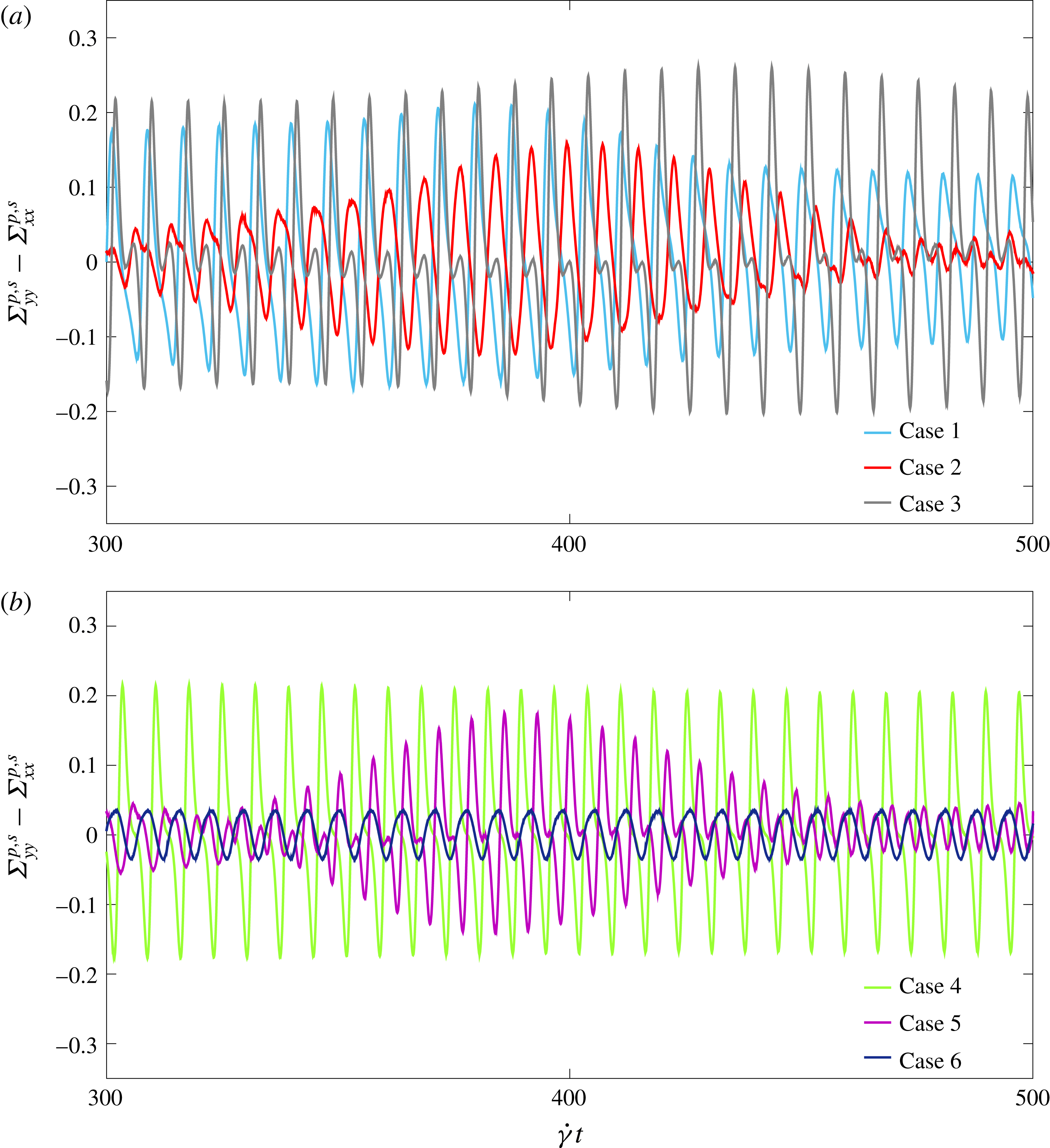
 $\unicode[STIX]{x1D6F4}_{zz}^{p,s}-\unicode[STIX]{x1D6F4}_{yy}^{p,s}$
is shown as a function of time for two irregular-shaped particles (a)
 $\beth$
and (b)
 $\aleph$
. Except for the case 6 (which is always a negative value) the first normal stress difference oscillates between positive and negative values with a negative cycle average.

Instantaneous second normal stress difference
 $\unicode[STIX]{x1D6F4}_{yy}^{p}-\unicode[STIX]{x1D6F4}_{xx}^{p}$
is shown as a function of orientation for two complex-shaped particles (a)
 $\beth$
and (b)
 $\aleph$
. The second normal stress difference oscillates between positive and negative values with a positive cycle average.

Results for instantaneous first and second normal stress differences are plotted as a function of time for both particles and different initial orientations in figures 10 and 11, respectively, and their averaged values are presented in table 3. As expected, the tumbling motion of particles during cycles of rotation makes the behaviour of these variables oscillatory, similar to the shear stress. It can be observed, except for the first normal stress difference in case 6 (which is always a negative value), instantaneous normal stress differences oscillate between positive and negative values with comparable amplitudes. Additionally, for both particles, initial orientation has a drastic role on the amplitude of oscillations and can increase or decrease the amplitude of both normal stress differences by more than a factor of five (see for instance case 4 and case 6 in figures 10
b and 11
b for particle
 $\aleph$
). Also, similar to the shear stresslet, the time history of normal stress difference reveals that the amplitude of oscillations is sensitive to orbital change, and a small variation in angular velocity can result in a significant change in normal stress differences – see the second normal stress difference for cases 2 and 5 in figure 11 and compare them with their angular velocities in figure 5.
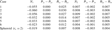
These normal stress differences, as can be seen in table 3, have negative and positive average values, respectively, and
 $N_{1}$
has a significantly higher absolute value compared to
 $N_{2}$
. This is in agreement with the results of Rallison (Reference Rallison1978), which predicted a negative
 $N_{1}$
and positive
 $N_{2}$
(
 $|N_{1}|>|N_{2}|$
) for spheroids with aspect ratios less than five in a Brownian dilute suspension assuming Stokes flow. However, Kumar & Higdon (Reference Kumar and Higdon2011b
) found both normal stress differences negative, with two orders of magnitude lower absolute values for
 $\unicode[STIX]{x1D719}=0.05$
for three dicolloidal particle shapes (effective aspect ratio
 $1.08<r_{e}<1.51$
) in a non-Brownian suspension, again assuming Stokes flow. This could be due to the inertial effects and/or relatively simpler shape of particles compared to ours. Negative values of
 $N_{1}$
and positive values of
 $N_{2}$
are also in agreement with our previous results for spheroids at a similar volume fraction and Reynolds number (Daghooghi & Borazjani Reference Daghooghi and Borazjani2015b
). A result for a prolate spheroid (
 $r_{e}=2$
) from our previous publication is shown in table 3 for comparison. In fact, the first normal stress difference of particle
 $\aleph$
is close to a spheroid with an aspect ratio of
 $r_{e}=2.0$
, while particle
 $\beth$
has a significantly higher value (50 % more); i.e., its value is higher than the spheroid with
 $r_{e}=3.0$
(
 $N_{1}=-0.018$
) but lower than the one with
 $r_{e}=5.0$
(
 $N_{1}=-0.081$
) (Daghooghi & Borazjani Reference Daghooghi and Borazjani2015b
). On the other hand, the second normal stress differences for both particles are within the same range and close to the results of spheroids with an aspect ratio
 $r_{e}=2.0$
.
First and second normal stress differences (
 $N_{1}$
and
 $N_{2}$
), and contribution of acceleration stress (
 $\bar{\unicode[STIX]{x1D617}}_{zz}-\bar{\unicode[STIX]{x1D617}}_{yy}$
,
 $\bar{\unicode[STIX]{x1D617}}_{yy}-\bar{\unicode[STIX]{x1D617}}_{xx}$
) and Reynolds stress (
 $\bar{\unicode[STIX]{x1D619}}_{zz}-\bar{\unicode[STIX]{x1D619}}_{yy}$
,
 $\bar{\unicode[STIX]{x1D619}}_{yy}-\bar{\unicode[STIX]{x1D619}}_{xx}$
) in their total values.

For normal stress differences, interestingly and in contrast to the shear particle stress, the role of Reynolds stress and acceleration stress is not negligible. Our calculations show that these parts of the particle stress differences have significantly lower amplitudes with respect to the stresslet part, but their averaged values can have a drastic impact on
 $N_{1}$
and
 $N_{2}$
. For the first normal stress difference
 $N_{1}$
, the acceleration stress has almost zero contribution (in agreement with our previous results for spheroids (Daghooghi & Borazjani Reference Daghooghi and Borazjani2015b
), e.g.,
 $r_{e}=2$
in table 3), whereas the Reynolds stress difference has an average value comparable to the stresslet term (in case 2 and case 6 its value is equal or even higher than stresslet contribution). Note that Reynolds stress has a negative contribution to normal stress differences based on (2.5). As the first stresslet difference is also a negative value, this mechanism of stress generation decreases the first normal stress difference further, and increases the amplitude of
 $\unicode[STIX]{x1D6F4}_{zz}-\unicode[STIX]{x1D6F4}_{yy}$
and
 $N_{1}$
. In contrast, the acceleration stress is not a negligible term for the second normal stress difference
 $N_{2}$
. As can be clearly seen in table 3,
 $\bar{\unicode[STIX]{x1D617}}_{yy}-\bar{\unicode[STIX]{x1D617}}_{xx}$
is a negative parameter for all cases and its value is less than one-half of the second Reynolds stress difference
 $\bar{\unicode[STIX]{x1D619}}_{yy}-\bar{\unicode[STIX]{x1D619}}_{xx}$
. The sign and the value of acceleration stress for both particles are consistent with our simulations for spheroids (table 3). Comparing the presented results with the previous ones for spheroids, the main difference is that for irregular particles the Reynolds stress term dominates the acceleration term in the second stress difference, whereas for spheroids both terms are equal and opposite. Consequently, Reynolds stress and acceleration stress cannot cancel out each other, and Reynolds stress dampen the amplitude of the second stress difference. In fact, we can see that the Reynolds stress has an opposite effect on the absolute value of
 $N_{1}$
and
 $N_{2}$
; i.e., it increases the absolute value of the former but decreases the absolute value of the latter.
6 Conclusion
We investigated the role of a particle’s shape on the rheological parameters of suspensions of irregular-shaped particles to assess the accuracy of approximating irregular particles with simplified geometries. To do so, we picked two different particle shapes (figures 1 and 2) and compared them against their equivalent spheroids.
For each particle, we initially oriented the particle at three different angles to make six test cases; in each case, numerical simulations were conducted to determine the orbit periods, and, hence, to find the effective aspect ratio. Our calculations showed all cases have close orbit periods and aspect ratios of approximately
 $1.5<r_{e}\leqslant 2$
based on both kinematics or geometric considerations, as discussed in § 2.4. We found that despite qualitative similarities between the rotation of an irregular-shaped particle and a spheroid, irregular-shaped particles have a more complicated rotation behaviour. Depending on their initial orientation, a complex kayaking motion with significant cycle-to-cycle variation can be seen for both particles. Contrary to a spheroid (Subramanian & Koch Reference Subramanian and Koch2005, Reference Subramanian and Koch2006; Dabade et al.
Reference Dabade, Marath and Subramanian2016), our results for angular velocity do not predict a migration towards a preferred orbit of rotation, and our initial-dependence results are more compatible with the bifurcation phenomenon observed in higher-Reynolds-number (Yu et al.
Reference Yu, Phan-Thien and Tanner2007; Rosén et al.
Reference Rosén, Lundell and Aidun2014, Reference Rosén, Do-Quang, Aidun and Lundell2015a
,Reference Rosén, Do-Quang, Aidun and Lundell
b
,Reference Rosén, Einarsson, Nordmark, Aidun, Lundell and Mehlig
c
) and doubly periodic/unstable motion of a triaxial ellipsoid (Hinch & Leal Reference Hinch and Leal1979; Yarin et al.
Reference Yarin, Gottlieb and Roisman1997).
We found that the particle stress depends on both initial orientation and particle shape, and its value can considerably change when particles rotate in different orbits. Based on our calculations for two irregular particles, the average shear particle stress is 20 %–120 % higher than the maximum value for their equivalent spheroidal particles, and it is closer to spheroids with higher aspect ratios (Mueller et al.
Reference Mueller, Llewellin and Mader2010; Daghooghi & Borazjani Reference Daghooghi and Borazjani2015b
). We showed that slenderness of a particle (high surface to volume) and mass distribution further from the centre of mass (moment of inertia around the vorticity direction per unit volume) can significantly (more than twice for an irregular particle and five times for a hollow cylinder) increase the average particle stress and consequently intrinsic viscosity relative to their equivalent spheroids. Such higher values of shear particle stress (intrinsic viscosity) indicate that approximation of irregular particles with simplified geometries, such as spheres or spheroids, may lead to similar levels of error in rheological properties of a suspension. The physical effect of these geometric factors on the rheology of a suspension is verified by systematically changing these geometric parameters on two mathematically defined families of particles (figure 8). We showed that shear particle stress is independently correlated with dimensionless
 $A_{p}/V_{p}$
and
 $I_{xx}/V_{p}$
(both parameters are non-dimensionalized by the one-half the largest diameter of the particle), and particles with higher values of these factors have a significantly higher particle stress (intrinsic viscosity).
Finally, normal stress differences for all cases are computed and compared with available numerical simulations. We observed that the first normal stress difference is negative for all cases, with higher absolute values for the slender particle, whereas the second normal stress difference is positive and also higher for the same particle. As expected, we noticed that the absolute value of the first normal stress difference is significantly higher than the second normal stress difference for all cases. We also found that, contrary to shear particle stress, acceleration stress and especially Reynolds stress are important mechanisms of stress generation and cannot be ignored in the calculation of particle stress differences. These terms can have average values comparable to the stresslet term and effectively increase
 $\Vert N_{1}\Vert$
or decrease
 $\Vert N_{2}\Vert$
, whereas their shear values are negligible compared to the shear stresslet, and cancel out each other when calculating shear particle stress
 $\bar{\unicode[STIX]{x1D6F4}}_{yz}^{p,s}$
similar to spheroids (Daghooghi & Borazjani Reference Daghooghi and Borazjani2015b
).
All the above results are obtained by assuming particles are initially oriented identically for each case – i.e., we picked a particle and implemented periodic boundary conditions. Such simulations for a periodic suspension are still a good approximation for a suspension in the dilute regime, because in this regime the interaction between particles is low similar to previous work (Huang et al.
Reference Huang, Wu and Lu2012a
; Rosén et al.
Reference Rosén, Do-Quang, Aidun and Lundell2015a
,Reference Rosén, Do-Quang, Aidun and Lundell
b
,Reference Rosén, Einarsson, Nordmark, Aidun, Lundell and Mehlig
c
; Daghooghi & Borazjani Reference Daghooghi and Borazjani2015b
). Additionally, for each tested particle in our study, we just considered three different initial orientations and observed a range of values for each viscometric function (e.g., intrinsic viscosity). However, in a real suspension, different particles have different initial orientations and the rheological parameters should be calculated by averaging over all particles’ values. Nevertheless, our results for all test cases show that shear particle stress and intrinsic viscosity are significantly higher than the maximum value of their equivalent spheroids at similar
 $Re$
and
 $\unicode[STIX]{x1D719}$
– i.e., the combination of them should have a higher value as well. Therefore, the current methods of defining equivalent particles for irregular ones underestimate rheological properties. Our results can lead to better equivalent models for irregular particles in the future.
Acknowledgements
This work was supported by the American Chemical Society (ACS) Petroleum Research Fund (PRF) grant no. 53099-DNI9. The computational resources were partly provided by the Center for Computational Research (CCR) at the University at Buffalo.
Supplementary movie
A supplementary movie is available at https://doi.org/10.1017/jfm.2018.65.