


I. Introduction
The impact of the local culture on firms’ decisions is of growing interest in finance.Footnote 1 Culture’s effect on individuals’ trust is particularly relevant to understanding financial interactions between counterparties, since trust is central to these relationships and financial transactions (Arrow (Reference Arrow1972), Guiso, Sapienza, and Zingales (Reference Guiso, Sapienza and Zingales2004), (Reference Guiso, Sapienza and Zingales2008)). Cultural institutions, such as religions, shape individuals’ trust, which in turn affects local economic activity, for example, growth and investment (Knack and Keefer (Reference Knack and Keefer1997)). Despite this recognized importance, it is inherently difficult to identify plausibly causal links between culture, trust, and economic decisions because culture and the institutions that embody it are endogenous to the environment and generally very slow-changing. Drawing on the large literature on the role of religion in shaping cultural norms (North (Reference North2012), Putnam, Leonardi, and Nonetti (Reference Putnam, Leonardi and Nonetti1994), Guiso, Sapienza, and Zingales (Reference Guiso, Sapienza and Zingales2003), and Enke (Reference Enke2019)), we address this empirical challenge by focusing on scandals affecting the Catholic Church. This identification strategy allows us to analyze the impact of cultural institutions on interfirm financial cooperation.
In January 2002, the Boston Globe’s Spotlight article series revealed systematic organizational misconduct by Boston’s Catholic Church leader (bishop). The articles detailed how the bishop of Boston reassigned clergy whom he knew to have a history of child abuse to different churches—where they were likely to be in proximity with children and, indeed, committed more abuse. The Spotlight news articles set off a wave of disclosures of past abuse by Catholic clergy in various parts of the United States. These events damaged trust in local Catholic Church organizations and their leadership that knowingly relocated accused clergy (Bruce (Reference Bruce2011), Esparza (Reference Esparza2020)). The scandal also reduced Catholics’ religious participation and charitable donations to Catholic organizations (Hungerman (Reference Hungerman2013), Bottan and Perez-Truglia (Reference Bottan and Perez-Truglia2015)). That is, the scandal presented a consequential negative shock to an important religious and cultural institution for affected communities.
We expect this negative shock to translate into changes in cooperative behavior, drawing from prior work: Putnam, Leonardi, and Nonetti (Reference Putnam, Leonardi and Nonetti1994) and Putnam (Reference Putnam2000) see participation in cultural activities as a means of building cooperation and trust. Fukuyama (Reference Fukuyama1995) underscores cultural institutions’ role in fostering cooperation and building trust as an important determinant of firms’ decisions and success, while LaPorta, de Silanes, Shleifer, and Vishny (Reference LaPorta, de Silanes, Shleifer and Vishny1997) illustrate the role of religion in this regard. Previous literature also highlights how religion affects individuals’ work decisions (Buren, Syed, and Mir (Reference Buren, Syed and Mir2020), Weaver and Agle (Reference Weaver and Agle2002)) due both to its role in shaping social norms and to the impact of religious moral authority (McGuire, Omer, and Sharp (Reference McGuire, Omer and Sharp2012), Peifer (Reference Peifer2015)). The scandal, laying bare moral breaches on the part of some of the Catholic Church’s local leaders, weakens the Church’s moral authority and its standing in the community. Accordingly, we predict that the Catholic Church scandal will have significant spillover effects on the individuals working in firms in affected communities, negatively impacting those firms’ cooperative behavior toward counterparties.
To support this intuition, we document in survey data that trust in religious institutions correlates with trust in businesses and that individuals in communities most affected by the scandals report lower levels of confidence in both the clergy and business. These findings demonstrate how negative religious shocks can transmit trust spillovers into individuals’ economic dealings, motivating our analysis of interfirm cooperative impacts.
We examine the effects of religious shocks on interfirm relationships in the context of supply chain interactions. As our outcome of interest, we focus on firms’ provision of trade credit, the informal short-term lending that takes place when firms sell products or services to customers on credit. Extending trade credit explicitly creates a financial vulnerability for the seller, exposing the firm to repayment risk and magnifying the potential for adverse supply chain spillovers (e.g., Hertzel, Li, Officer, and Rodgers (Reference Hertzel, Li, Officer and Rodgers2008), Boissay and Gropp (Reference Boissay and Gropp2013), Jacobson and Von Schedvin (Reference Jacobson and Von Schedvin2015), and Murfin and Njoroge (Reference Murfin and Njoroge2015)).Footnote 2 Thus, the provision of trade credit requires the supplier’s willingness to accept this risk, engage in cooperative behavior, and trust its customers (Guiso, Sapienza, and Zingales (Reference Guiso, Sapienza and Zingales2004)).Footnote 3 Indeed, previous work has used a firm’s extension of trade credit to a customer to measure trust (see McMillan and Woodruff (Reference McMillan and Woodruff1999)).
Consistent with our predictions, we find that firms in communities most affected by the religious scandal subsequently reduced their provision of trade credit to major customers. These effects are most pronounced in relationships in which trust is more crucial.
We are able to precisely measure trade credit provision with a granular database of pair-level trade credit between U.S. publicly traded firms (Ersahin, Giannetti, and Huang (Reference Ersahin, Giannetti and Huang2024), Freeman (Reference Freeman2025a), and Billett, Freeman, and Gao (Reference Billett, Freeman and Gao2026)). In contrast to most studies examining firm-level trade credit balances (i.e., aggregated across supply chain partners), the advantage of this data set is its pairwise nature. This feature allows us to make detailed inferences about changes in trade credit provision to individual customers following cultural shocks while controlling for demand-side factors and firm characteristics.Footnote 4
To identify areas impacted by this scandal, we use news revelations of a bishop’s disciplinary measures against clergy accused of abuse: their removal from active ministry. These removals of clergy from active ministry are the belated acknowledgment of a breach in governance by local Catholic Church leaders, signifying that members of the local clergy who should not be ministering to local Catholics were allowed to do so for some time. We read through news articles mentioning removals of Catholic clergy based on claims of abuse, creating an indicator for regions where newspapers report clergy removals from ministry. In the wave of such revelations between 2002 and 2004, we identify 113 Catholic regions (“dioceses”) impacted by the scandal, out of 176 dioceses in the United States. These treated areas cover 52% of U.S. counties, a geographically diverse span of the country as evidenced by Figure 2. Besides its cross-sectional variation across well-defined areas, the Catholic clergy abuse scandal offers several empirical advantages as a shock to local cultural institutions. First, the decision to remove a clergy member stems from allegations whose timing is not controlled by the firm or by the Catholic church, generally based on decades-old events (John Jay College of Criminal Studies (2004)). Second, Catholicism is a large religion in the United States, making it a culturally relevant institution. Third, because Catholic dioceses are a collection of nonoverlapping counties, we can differentiate between areas where the scandal is likely to inflict greater damage to the local culture (counties where Catholicism’s influence is stronger) and areas where the scandal is less likely to have a pervasive local impact (counties where Catholic influence is more diffuse).Footnote 5
Because we expect the Catholic clergy abuse scandal to affect communities most strongly where Catholicism is more prevalent and culturally formative, we use a triple-difference approach using a stacked sample around the staggered timing of the religious scandals, with the triple-difference estimator focusing on firms located in highly Catholic counties subject to the shock after the scandal revelations. This empirical design offers another strength: Any confounding event during the post-abuse crisis period would have to specifically affect firms located in Catholic-intensive counties in order to bias these estimates.Footnote 6 This greatly reduces the probability that our triple interaction term of interest systematically captures an effect not associated with the Catholic abuse crisis itself. We find that firms in areas most heavily affected by the scandal decrease their provision of trade credit by 5.3%–5.9% of sales. Dynamic triple-difference estimation shows that treated firms reduce their extension of trade credit starting in the year of the scandal, with levels remaining low in subsequent years.
Following previous studies on the relationship between cultural institutions and trust (Putnam, Leonardi, and Nonetti (Reference Putnam, Leonardi and Nonetti1994), Fukuyama (Reference Fukuyama1995)), we hypothesize that the most likely mechanism between the cultural shock and the decrease in trade credit is social capital, which Woolcock (Reference Woolcock1998) defines as the norms of cooperation shared by members of a community. To test the social capital channel, we investigate whether results vary with the importance of trust between supply chain partners. Giannetti and Wang (Reference Giannetti and Wang2016) argue that negative shocks to trust are more likely to affect counterparties that are harder to monitor, that is, those for whom social capital plays a greater role in ensuring cooperation. We find evidence consistent with the social capital channel: Firms lower trade credit to customers who are lesser known and farther away or when the relationship is more operationally complex.
Our trade credit results are robust to a battery of alternative specifications and tests: We find that the magnitude of the effect is similar between earlier and later treated cohorts. Results hold for single-segment firms, alleviating concerns about geographic dispersion within firms. Moreover, our results are robust to the inclusion of entropy-balanced controls and to an alternative definition of strongly Catholic-influenced areas. We find consistent results in difference-in-differences estimations between treated and untreated firms within the subsample of heavily Catholic counties, as well as between firms in Catholic counties (subsequently referred to as “Catholic firms” for brevity) and non-Catholic counties within the subsample of firms in scandal-affected areas. One concern could be that the scandals adversely affect firms’ financial ability to extend credit, but we find no evidence of any adverse effects on affected firms’ financial standing. Finally, our estimation design greatly mitigates concerns about alternative explanations: First, since we focus on a 7-year window (3 years pre- and post-event) around the initial news of clergy removals, we avoid the effect of the 2008 Financial Crisis. In addition, our results are unlikely to be driven by industry-specific shocks, as we include specifications with industry-year fixed effects throughout our analysis.
This paper offers new, plausibly causal evidence on the influence of the local culture on interfirm relationships, contributing to the literature in several ways. First, we exploit quasi-exogenous shocks to show causal evidence of the role of local culture on firm behavior. Shocks to local culture are rare, but the Catholic clergy scandal allows us to observe the effects of a shock to the firm’s environment exogenous to the firm. Two related papers are Hilary and Huang (Reference Hilary and Huang2023), who study the effect of the Catholic scandals on sporadic contracting decisions within the firm, and D’Acunto, Xie, and Yao (Reference D’Acunto, Xie and Yao2022), who find that corporate scandals affect trust in corporate consulting contracts. Distinct from these prior works, we offer evidence that shocks to local cultural institutions also affect local firms’ recurring interactions with supply chain counterparties (external to the firm). Further, our results point to a specific social capital channel through which the shock to trust in the Catholic Church affects local firms’ supply chain relationships.Footnote 7
Second, we contribute to the literature on local culture and trust. The traditional view on culture is that the values and beliefs it embodies are very slow-moving (Putnam, Leonardi, and Nonetti (Reference Putnam, Leonardi and Nonetti1994), Fukuyama (Reference Fukuyama1995)). By contrast, a strand of literature finds that social connections (Duflo and Saez (Reference Duflo and Saez2002), (Reference Duflo and Saez2003), Hong, Kubik, and Stein (Reference Hong, Kubik and Stein2004)) and shocks to religious identity (Benjamin, Choi, and Fisher (Reference Benjamin, Choi and Fisher2016), Bryan, Choi, and Karlan (Reference Bryan, Choi and Karlan2020)) can impact individuals’ behavior very swiftly. Accordingly, new theory highlights the possibility of rapidly changing cultural attitudes (Acemoglu and Robinson (Reference Acemoglu and Robinson2025)). Consistent with these latter papers, we find evidence that changes in local cultural institutions quickly alter firm behavior toward their counterparties. Moreover, with our focus on ongoing relationships between supply chain partners, this study is distinct from papers that focus on the impact of cultural norms on rare firm events, such as mergers and acquisitions (e.g., Ahern, Daminelli, and Fracassi (Reference Ahern, Daminelli and Fracassi2015)).
Third, we contribute to a stream of papers examining the role of nonpecuniary factors in trade credit decisions, such as bargaining power (e.g., Klapper, Laeven, and Rajan (Reference Klapper, Laeven and Rajan2012), Murfin and Njoroge (Reference Murfin and Njoroge2015), Fabbri and Klapper (Reference Fabbri and Klapper2016), and Billett, Freeman, and Gao (Reference Billett, Freeman and Gao2026)) and competition (e.g., Chod, Lyandres, and Yang (Reference Chod, Lyandres and Yang2019), Giannetti, Serrano-Velarde, and Tarantino (Reference Giannetti, Serrano-Velarde and Tarantino2021)). Particularly relevant to our setting, Giannetti, Burkart, and Ellingsen (Reference Giannetti, Burkart and Ellingsen2011) and Dass, Kale, and Nanda (Reference Dass, Kale and Nanda2015) show that trade credit use is higher in relationships requiring more collaboration. McMillan and Woodruff (Reference McMillan and Woodruff1999) use the decision to extend trade credit as a measure of customer trust, and Antras and Foley (Reference Antras and Foley2015) show repeated interactions foster cooperation in import–export relationships. We contribute to this area of the trade credit literature by showing plausibly causal evidence of how the cultural environment in which the firm operates affects the provision of credit.
Two particularly related papers are Wu, Firth, and Rui (Reference Wu, Firth and Rui2014) and Levine, Lin, and Xie (Reference Levine, Lin and Xie2018). Both papers show greater use of trade credit by constrained firms in high-trust regions, emphasizing how trade credit can smooth financial frictions in these locations. We differ by abstracting away from financial constraints and studying how shocks to local cultural institutions shape trade credit decisions (outside of a crisis setting). Since societal patterns like norms of trust are long-standing and likely correlated with other social and economic patterns, our work shows a plausibly causal relationship via an adverse shock to trust in cultural institutions. Our results also differ by showing a complementary relationship between trust in institutions and trade credit extension: While Wu, Firth, and Rui (Reference Wu, Firth and Rui2014) and Levine, Lin, and Xie (Reference Levine, Lin and Xie2018) show that lower trust in financial and political institutions increases trade credit usage, we find that a decrease in trust in cultural institutions reduces trade credit. Our setting also allows us to focus on a shock affecting a set of firms with a more homogeneous legal environment (all U.S. firms). Thus, our study highlights the role of trust in trade credit decisions even in an environment with relatively stronger legal protections and financial access.
II. Background: Religious Scandals, Trust, and Trade Credit
This section provides motivation from the literature to show i) how a negative shock to cultural institutions would affect interfirm decisions involving trust and ii) why trade credit extension is a good laboratory for examining such interfirm decisions.
A. Religious Scandals and Firm Decision-Making
Cultural institutions instill norms and beliefs that affect individuals’ willingness to trust (e.g., Fukuyama (Reference Fukuyama1995)). Trust, in turn, impacts business judgment in day-to-day operations: For example, Pursiainen (Reference Pursiainen2022) finds evidence that equity analysts’ opinions are affected by their country’s cultural biases toward the country of the firm they evaluate. Rothstein and Stolle (Reference Rothstein and Stolle2008) underscore the importance of ethical behavior by leaders of local institutions to foster trust: Individuals infer that “if those in positions of authority cannot be trusted, then most other people can surely not be trusted” (p. 446).
Following a large literature, we focus on religion as an important cultural institution (e.g., Putnam, Leonardi, and Nonetti (Reference Putnam, Leonardi and Nonetti1994), Putnam (Reference Putnam2000), and Hong, Kubik, and Stein (Reference Hong, Kubik and Stein2004)). Religion has a positive impact on individuals’ trust (Guiso, Sapienza, and Zingales (Reference Guiso, Sapienza and Zingales2003)), which decreases contract enforcement costs (North (Reference North2012), Knack (Reference Knack2001)). Employees’ religion plays an important role in shaping their ethical behavior in the workplace (Buren, Syed, and Mir (Reference Buren, Syed and Mir2020), Weaver and Agle (Reference Weaver and Agle2002)). This influence is ascribed to the weight that religious values bear on individuals’ decisions, through the importance of religious tenets in local social norms and the moral authority of religious institutions (McGuire, Omer, and Sharp (Reference McGuire, Omer and Sharp2012), Peifer (Reference Peifer2015)). Conversely, ethical breaches by religious leaders constitute a negative shock to trust in religious authority for individuals in the local community, which we expect to negatively spill over into their business decisions. For example, Hilary and Huang (Reference Hilary and Huang2023) find that religious scandals lead to more stringent contracts for CEOs of local firms. Our hypothesis is related but distinct: First, we study the role of trust in counterparty relationships where contracts are part of the recurrent business of the firm, while Hilary and Huang (Reference Hilary and Huang2023) focus on the product of sporadic negotiations between the firm’s principals and their primary agent, the CEO. We look at relationships between the firm and outside parties (supply chain partners), while Hilary and Huang (Reference Hilary and Huang2023) study relationships internal to the firm, between the board and their top employee. Moreover, our results provide evidence of a social capital mechanism through which the shock to trust impacts local firms’ decisions. Finally, we study contracts for which enforcement provisions are generally implicit (and therefore highly dependent on the trade credit provider’s trust), whereas Hilary and Huang (Reference Hilary and Huang2023) focus on the characteristics of explicit provisions in compensation contracts (which are then subject to careful legal enforcement).
Since firms tend to hire locally, we expect religious scandals to impact local workers in communities where the religion is locally prevalent and, thus, has greater social weight (LaPorta, de Silanes, Shleifer, and Vishny (Reference LaPorta, de Silanes, Shleifer and Vishny1997), Stulz and Williamson (Reference Stulz and Williamson2003), and Kumar, Page, and Spalt (Reference Kumar, Page and Spalt2011)).Footnote 8 Prior literature shows that individual-level contextual factors affect firm performance. In addition to the cultural biases in analyst recommendations, as already discussed (Pursiainen (Reference Pursiainen2022)), employees’ cultural backgrounds influence workplace behaviors such as shirking and absenteeism (Ichino and Maggi (Reference Ichino and Maggi2000)). Also, personal life shocks affect both innovative productivity (Bernstein, McQuade, and Townsend (Reference Bernstein, McQuade and Townsend2021)) and investment decisions (Pool, Stoffman, Yonker, and Zhang (Reference Pool, Stoffman, Yonker and Zhang2019)). Since individuals’ decisions are influenced by external factors, we anticipate that a negative shock to trust in religious institutions would affect firm outcomes in the community via their employees.
While previous work considers the role of direct social ties between firms and the effects of managerial actions (e.g., Cline, Walkling, and Yore (Reference Cline, Walkling and Yore2018), Dasgupta, Zhang, and Zhu (Reference Dasgupta, Zhang and Zhu2021), and Liang, Cavusoglu, and Hu (Reference Liang, Cavusoglu and Hu2025)), we examine the role of local cultural institutions in interfirm cooperation. Our empirical design addresses the issue of endogenous cultural factors by focusing on a local shock to a large religious denomination, Catholicism, in areas where this religious denomination is prevalent. Our key hypothesis is that the adverse shock to trust in Catholic leadership affects decision-making in firm actions involving trust.
B. Trade Credit and Trust
In this section, we discuss the institutional background of trade credit in our empirical setting. We focus on the incomplete contracting and implicit nature of its use that mean relational factors (such as trust) can and do play an important role in trade credit decisions. Trade credit usage is widespread globally (e.g., Rajan and Zingales (Reference Rajan and Zingales1995)) and in the United States, where its volume is greater than 20% of gross domestic product (Garcia-Marin, Justel, and Schmidt-Eisenlohr (Reference Garcia-Marin, Justel and Schmidt-Eisenlohr2020)). Simultaneously, trade credit is governed under incomplete, largely informal contracts (Federal Reserve Board (2007), Malcomson (Reference Malcomson2012), Levine, Lin, and Xie (Reference Levine, Lin and Xie2018), and Macaulay (Reference Macaulay2018)).Footnote 9 For example, Macaulay (Reference Macaulay2018) notes the prevalence of ambiguously defined terms in vertical transactions, implicitly accompanied by an acknowledgment that the parties would negotiate if needed.Footnote 10 Indeed, many papers model trade credit as a way to help alleviate the problems of incomplete contracting implicit in supply chain transactions. Dass, Kale, and Nanda (Reference Dass, Kale and Nanda2015) and Kim and Shin (Reference Kim and Shin2012) model trade credit as a way of integrating the fortunes of firms along the supply chain to help align firm goals. Knack and Keefer (Reference Knack and Keefer1997) cite “[transactions] in which goods and services are provided in exchange for future payment” (p. 1252) as an example of trust-intensive contracts. Related, Cai, Quan, and Tian (Reference Cai, Quan and Tian2023) find that corruption, which weakens trust between counterparties, is negatively correlated with the use of trade credit, illustrating the role that trust plays in the provision of trade credit.
Why does trade credit extension involve supplier trust? Trade credit in the United States is regulated under various state laws following the Uniform Commercial Code (UCC). The UCC specifies that trade credit must be agreed upon and ensures the seller’s rights to assurance of performance, reclamation of goods, and legal recourse to sue for receivables enforcement. Thus, from a strictly legal standpoint, suppliers seemingly have at least some degree of recourse for defaulted payment. Indeed, several early papers examining the rationale for the existence of trade credit postulated that suppliers may have a lending advantage over banks due to their superior ability to redeploy collateral in the case of default (e.g., Frank and Maksimovic (Reference Frank and Maksimovic1998), Fabbri and Menichini (Reference Fabbri and Menichini2010)). In reality, however, practical and market factors limit the extent to which these provisions protect sellers from default or late payment. Confiscating unpaid-for products is challenging (at best) once the goods have been transformed or sold, and, by definition, impossible for firms supplying services rather than physical products (Costello (Reference Costello2019)). Even in cases where seizing collateral is technically possible, the window in which it can be done is limited. Prior to 2006, the reclamation period for goods sold on credit was 10 days under the UCC. Costello (Reference Costello2019) shows that after a U.S. legal change increased the reclamation period for reclaiming goods sold to 45 days,Footnote 11 firms extended more credit to riskier customers. However, even a 45-day window typically closes before the end of terms typically observed for firms in Compustat (e.g., the mean number of days outstanding in our sample is 63 days of sales).Footnote 12 Thus, given logistical and legal challenges, the ability to seize collateral in the event of default is tenuous.
Further, while default is a major risk in extending credit, so is late payment. Cowton and San-Jose (Reference Cowton and San-Jose2017) discuss payment length as an ethical dimension of trade credit, emphasizing the importance of the informal promise of payment between counterparties. Late payment practices are common: Ng, Smith, and Smith (Reference Ng, Smith and Smith1999) find in survey results that important customers often delay payment past terms without penalty, and Klapper, Laeven, and Rajan (Reference Klapper, Laeven and Rajan2012) find that large, financially secure firms receive the most favorable terms from suppliers.Footnote 13 Murfin and Njoroge (Reference Murfin and Njoroge2015) show that suppliers can become financially constrained after being forced to accommodate unilateral changes in payment policy of downstream buyers with significant bargaining power. Thus, given that large customers frequently abuse terms due to bargaining power, suppliers face risks regarding timely payment, even from customers of high credit quality.Footnote 14
In summary, given the informality frequently implicit in trade credit agreements, high potential costs of default or late payment, and limitations in legal recourse, relational factors will influence decisions to extend trade credit. Extending trade credit to a customer explicitly creates a financial vulnerability, exposing the supplying firm to repayment risk and magnifying the potential for adverse supply chain spillover (Hertzel, Li, Officer, and Rodgers (Reference Hertzel, Li, Officer and Rodgers2008), Boissay and Gropp (Reference Boissay and Gropp2013), and Jacobson and Von Schedvin (Reference Jacobson and Von Schedvin2015)). By focusing on religious scandals in the firm’s headquarter location, we exploit cultural shocks likely to affect trade credit decision makers, since receivables policy and credit decisions are typically set by middle management who are likely to work locally.Footnote 15 Particularly, a negative shock to supplier trust should adversely impact the extension of credit to a customer.
III. Shock to the Local Culture
A. Institutional Details
As a shock to trust in cultural institutions, we employ the Catholic clergy sexual abuse scandal triggered by the news revelations from the Boston Globe’s Spotlight team. In January 2002, this group of journalists documented that the head of the Catholic church for the Boston region, Cardinal Bernard Law, had reassigned priests whom he knew to have abused children in past assignments. These abuses took place decades earlier (most of the U.S. Catholic clergy abuses publicly disclosed as a result of this crisis occurred in the late 1960s and 1970s; see John Jay College of Criminal Studies (2004)). While the serial abuse by some of these priests was already known before 2002, the direct involvement of the local bishop in knowingly assigning priests accused of abuse was a thundering revelation to local Catholics.Footnote 16
Following these revelations, Catholic bishops in many parts of the United States were faced with the call to review the files of the priests and deacons in their regions in light of resurfaced past claims of clergy abuse of minors. These reviews led to the removal of some of these ministers from their current assignments. Clergy removals implicitly acknowledge the previous mishandling of abuse claims by the then-bishop: A priest who should not have been reassigned after claims of abuse decades prior had been allowed to keep working. Also, the removals present other advantages as a measure of the scandal. First, the removals are announced concurrently with the public disclosures of allegations against the clergy member. Therefore, the removals reveal the presence of a potentially hurtful clergy member in a church community (and in the communities where he worked previously).Footnote 17 Second, they only occur if allegations of abuse by a given clergy are credible, corresponding to a high “signal-to-noise” ratio relative to allegations themselves. Third, because removals require that a clergy member be actively working, they are much more salient to the local Catholic population than allegations against a long-ago retired, defrocked, or deceased priest. Removals make it clear to the local Catholic population that, though most instances of abuse occurred decades prior, bishops’ mishandling of those claims has lingering consequences to date.
Bruce (Reference Bruce2011) details how this scandal eroded Catholics’ trust in their local Church leaders. Hungerman (Reference Hungerman2013) offers evidence that Catholics in regions affected by these revelations left their Church, while Bottan and Perez-Truglia (Reference Bottan and Perez-Truglia2015) find that local households reduced religious participation and charitable giving. The scandal also lowered attendance in Catholic schools (Esparza (Reference Esparza2020)). Given that religious leaders are often seen as models of moral behavior (Weber (Reference Weber, Roth and Wittich1978), Rothstein and Stolle (Reference Rothstein and Stolle2008)), we posit that the Catholic clergy abuse scandal, which damaged trust in the Catholic Church and its leadership, is likely to have spillover effects to trust in interfirm cooperation. We hypothesize that this shock will be most salient in areas where the Catholic culture is more prevalent.
Even within their Church, Catholics’ behavioral shifts appeared to be specifically directed toward bishops—the leaders who violated their trust by reassigning accused priests. For example, Esparza’s (Reference Esparza2020) finding of lower school attendance is limited to Catholic schools under the purview of the bishop. By contrast, Esparza does not find a significant effect of the scandal on attendance in schools supervised by other Catholic entities (viz. religious orders). Moreover, within dioceses, Catholics treat their bishop and local priests differently: They pulled back from their relationship with the former but not with the latter.Footnote 18 Following these findings, we view shocked Catholics’ behavior as a redeployment of cooperative relationships away from the higher echelons of the Catholic Church, where trust is more costly, and toward closer, easier-to-monitor, representatives. This pattern is consistent with local Catholics investing less in relationships where trust is costlier.
The Catholic abuse scandal damaged trust in an influential local institution. Similar to work finding that workers’ culture influences their views of other firms (as discussed in Section II.A), our hypothesis is that this scandal affected individuals’ cooperative behavior toward their firms’ counterparties. This hypothesis is consistent with (while distinct from) prior work showing that the scandal revelations affected financial transactions, including CEO compensation (Hilary and Huang (Reference Hilary and Huang2023)) and stock market participation, a financial activity heavily dependent on trust and cooperation (Guiso, Sapienza, and Zingales (Reference Guiso, Sapienza and Zingales2004), (Reference Guiso, Sapienza and Zingales2008), Dupont (Reference Dupont2025)).
B. Motivating Evidence
To validate the conjecture of a spillover effect from trust in religious institutions to trust in a business context, we analyze the General Social Survey’s questions on confidence in various institutions over the years of our sample period (GSS survey years 1998–2006). In particular, we focus on two questions: i) confidence in churches and religious organizations and ii) confidence in large businesses. For each of these questions, respondents can answer whether they have a “great deal,” “only some,” or “hardly any” confidence in the organization. We create variables based on these answers: Confidence_Rel (Confidence_Bus) is set to 1 if a respondent answers that they have “a great deal” of confidence in churches and religious institutions (large businesses), 0 if they answer the “only some,” and −1 if they answer “hardly any.” We then estimate the equation:

for respondent
$ i $
 in year
$ t $
 . We include year and county (
$ c $
 ) fixed effects based on the GSS restricted localization data.
$ {X}_{i,t} $
 is a vector of controls that include the respondent’s age, demographic characteristics (gender, education, race, as well as marital, employment, and health statuses), political preference, and (quintiles of) income and socioeconomic position. In our strictest specification, we also control for the respondent’s propensity to trust strangers. This variable helps isolate the correlation between confidence in business and religion by controlling for individuals’ general willingness to trust.
Figure 1 presents the point estimates and confidence intervals for the coefficient of interest
$ \beta $
 from equation (1).Footnote
19 The tests show a positive and significant correlation between confidence in religious institutions and confidence in businesses, without controls (left), with the baseline controls in vector
$ {X}_{i,t} $
 (middle), and with the baseline controls augmented by the respondent’s propensity to trust strangers (right). In all cases, the correlation between trust in religious organizations and in businesses is positive and statistically significant. In untabulated tests, we verify that these results hold across subsamples regardless of Catholic affiliation, in both treated and nontreated areas and both before and after the scandals. Admittedly, this evidence is correlative rather than causal. In this regard, our triple-difference estimation method is particularly helpful. Since the Catholic Church scandal is a negative shock to the religious institution itself, our triple-difference setting captures the effect of this shock to trust in the Catholic Church on local individuals’ decisions. In Section IV.A.1, we use this triple-difference identification strategy to provide evidence that the Catholic scandal negatively impacts both confidence in religious organizations and confidence in business in areas affected by the Catholic Church abuse scandal.
In Figure 1, point estimates (blue bars) with 90% confidence intervals for the coefficients on confidence in religious institutions, following equation (1):
$ Confidence\_{Bus}_{i,t}={\alpha}_c+{\alpha}_t+\beta Confidence\_{Rel}_{i,t}+\gamma {X}_{i,t}+{\varepsilon}_{i,t} $
 , for respondent
$ i $
 in year
$ t $
 , between 1998 and 2006. The dependent variable captures confidence in large business organizations. We include year and county (
$ c $
 ) fixed effects based on the GSS restricted localization data. In the “Base Controls” specification,
$ {X}_{i,t} $
 is a vector of controls including the respondent’s age, demographic characteristics (gender, education, and race as well as marital, employment, and health statuses), political preference, and (quintiles of) income and socioeconomic position. On the right-hand side, we also include respondents’ propensity to trust strangers in the controls. All estimates use year and county fixed effects.

Figure 1 Long description
The chart presents three vertical bars, each representing a different model specification along the x-axis: No Controls, With Base Controls, and With Controls Including Trust in Strangers. The y-axis is labeled Coefficient, ranging from negative 0.05 to 0.25. The leftmost bar, labeled No Controls, has a coefficient near 0.2 with a magenta error bar extending above and below the top. The middle bar, labeled With Base Controls, has a coefficient near 0.15 with a similar error bar. The rightmost bar, labeled With Controls Including Trust in Strangers, also has a coefficient near 0.15 with an error bar. All bars are light blue. The chart title states Variable of Interest: Confidence in Religious Organizations and Dependent Variable: Confidence in Large Businesses. The coefficients decrease slightly as more controls are added, but remain positive and statistically significant.
As discussed in the evidence from Section III.A, the Catholic abuse scandals are a negative shock to trust in a prominent local religious institution. The results from Figure 1 show that trust in religious institutions and trust in businesses are highly correlated. This pattern suggests that a (negative) shock to trust in the Catholic Church could (negatively) impact Catholics’ trust in businesses, which would affect trade credit interactions between counterparties.Footnote 20
With this motivating evidence on the correlation between trust in religion and trust in businesses, and given previous findings on the effect of the Catholic clergy abuse scandal, we hypothesize that the scandal will reduce the willingness of local firms to cooperate with counterparties, especially for firms located in communities where Catholicism is prominent and in vulnerable settings where trust is important. Therefore, we expect the negative shock to the local culture to lead to more restrictive trade credit provision between the firm and its customers.
The most natural channel through which damaged trust in institutions would affect interfirm cooperation is via a reduction in social capital, that is, the norms of cooperation between parties (Knack and Keefer (Reference Knack and Keefer1997), Guiso, Sapienza, and Zingales (Reference Guiso, Sapienza and Zingales2004)). Alternative channels might also be at play, among which the leading candidates are risk aversion and financial deterioration. We test these alternative channels in Section VI and find no supporting evidence for either.Footnote 21 We do find evidence supporting the social capital channel: Firms particularly contract trade credit provision in customer relationships where trust is more important.
IV. Empirical Framework
A. Data
To analyze how a negative cultural shock affects the provision of trade credit, we first collect information from Factiva on the clergy removals discussed in Section III. We then merge the location and date of the removals with historical firm headquarter locations, using a panel of pair-level trade credit between U.S. publicly traded firms and their customers. The following sections describe our data composition in more detail.
1. Catholic Clergy Scandal and Local Catholic Population Data
We collect information about clergy removals through a search of news articles in Factiva based on a broad set of keywords between 2001 and 2007 (see Appendix B for more details). One diocese (Greensburg, PA) had a clergy removal in 2001 that was unrelated to the aftermath of the Spotlight news series; we exclude this diocese from the sample. The dioceses with removals in 2005 (e.g., Anchorage, AK; Honolulu, HI) include hardly any industrial activity. The news search yields no new dioceses with removals in 2006. Moreover, we exclude the dioceses impacted in 2007 from the treatment cohorts, since the post-impact analysis is potentially confounded by the effects of the financial crisis of 2008. As a result, we focus on the dioceses faced with removals between 2002 and 2004. In that span, 113 out of the 176 U.S. (Roman) Catholic regions (“dioceses”) were faced with clergy removals related to abuse claims, covering 52% of U.S. counties.Footnote 22
We mark these dioceses directly affected by the Catholic Church scandal with a “Removal” indicator. The “Post” indicator is set to 1 in the year of the removal. Figure 2 shows the U.S. regions impacted by Catholic clergy removals due to claims of abuse and the initial time of the announcement of the removals. The removals cover a diverse and significant portion of the country. We link diocese boundaries to U.S. counties using a diocese-county mapping file provided by the Center for Applied Research in the Apostolate (CARA) in Washington, D.C.
Figure 2 displays dioceses for which the measure of Removal turns to 1. Each color indicates the first year for which the indicator turns on. Years are indicated by the legend on the right.

Figure 2 Long description
Starting in the Northwest, counties are shaded by year: blue for 2001, red for 2002, orange for 2003, brown for 2004, green for 2005, and gray for 2007, as indicated by the legend at the right. Red, representing 2002, dominates the Midwest, Northeast, and parts of the South and West. Orange (2003) appears in clusters in the West, Midwest, and Northeast. Brown (2004) is scattered in the Midwest, South, and West. Green (2005) is seen in Alaska and a few counties in the Midwest and Northeast. Gray (2007) is present in the West, Midwest, and South. White counties indicate no removal measure. The map includes Alaska, where most of the state is green, and Hawaii, which is unshaded. The legend on the right lists years and corresponding colors.
To measure the prevalence of the local Catholic culture, we use an indicator set to 1 if the Catholic share of the population in a given county is above the population-weighted median among U.S. counties.Footnote 23 We obtain information on the Catholic local population from the 2000 survey of the Association of Religion Data Archives (2000) (ARDA). We refer to these areas where the Catholic Church is prevalent as “Catholic counties.”
Before turning to our primary focus on interfirm trade credit, we revisit the GSS data to provide evidence of how the scandal affected trust in religious institutions and large businesses. Following Hilary and Hui’s (Reference Hilary and Hui2009) and Hilary and Huang’s (Reference Hilary and Huang2023) work on the impact of religion on firms using the GSS, we collapse the data at the county-year level and interpolate the values of confidence in religious organizations, confidence in large businesses, and a similar set of controls to what we used in equation (1). With these interpolated data, we create a stacked sample for the event cohorts that we use in our main sample (i.e., 2002–2004), with the dioceses not treated during the event window as the control group.Footnote 24
To test the impact of the scandal on local confidence in religious and business institutions, we use the following triple difference estimation:

for county
$ c $
 , year
$ t $
 and event cohort
$ e $
 , where
$ I $
 refers to either religious institution or businesses.
$ \mathit{\operatorname{Re}}{movals}_{c,t} $
 is set to 1 if the county is located in a diocese with clergy removal, and
$ {Post}_{c,t} $
 is set to 0 prior to the initial removal in the diocese and 1 from that date. We ignore observations when the year of the survey is the year of the initial removal and estimate the effect for 3 years around the event year. We interact the county and year fixed effects with event cohort fixed effects and cluster errors at the diocese-event level.
The blue bars in Figure 3 represent the coefficients of the triple interaction term of interest (
$ {b}_1 $
 ). The two leftmost bars show the estimates for the confidence in churches and religious organizations outcomes, without and with controls. In both specifications, respondents in Catholic counties affected by the scandal display a significantly lower trust in churches and religious institutions. The two rightmost bars show a similar effect for confidence in large businesses, again both with and without controls.Footnote
25 The results emphasize the negative impact of the scandals on confidence in religious and business organizations in Catholic counties impacted by the scandal.
In Figure 3, point estimates (blue bars) with 90% confidence intervals for the coefficients on the triple interaction term of interest (
$ b1 $
 ) in equation (2):
$ Confidence\_{I}_{c,t}={a}_{c,e}+{a}_{t,e}+{b}_1{Post}_{c,t}\times {Catholic}_c\times {Removal}_{c,e}+{b}_2{Post}_{c,t}\times {Catholic}_c+{b}_3{Post}_{c,t}\times {Removal}_{c,e}+{c}_1{X}_{c,t}+{\unicode{x025B}}_{c,t,e} $
 , for respondents in county
$ c $
 in year
$ t $
 , in event cohort
$ e $
 . The index
$ I $
 on the dependent variable captures the type of institution concerned, namely, churches and religious organizations (two leftmost bars) or large business organizations (two rightmost bars). The unit of observation is a county-year, with interpolated values between survey years. We include event-year (
$ te $
 ) and event-county (
$ ce $
 ) fixed effects based on the GSS restricted localization data.
$ {X}_{i,t} $
 is a vector of controls including age, demographic characteristics (gender, education, and race, as well as marital, employment, and health statuses), political preference, and (quintiles of) income and socioeconomic position averaged by county-year.

Figure 3 Long description
The graph displays four vertical blue bars, each with a magenta confidence interval line. The x-axis is labeled Model, with four categories from left to right: No Controls and With Controls under Religious Organizations, then No Controls and With Controls under Large Businesses. The y-axis is labeled Triple Interaction Term Coefficient, ranging from 0.05 at the top to -0.6 at the bottom. All bars are below zero, indicating negative coefficients. The two left bars (Religious Organizations) are slightly more negative than the two right bars (Large Businesses). The confidence intervals for all bars extend well below zero, with the lowest points near -0.6. The top of each bar is close to -0.2. The graph suggests that the scandal reduced trust in both types of institutions in Catholic counties, regardless of controls.
2. Firms’ Trade Credit Provision
Our empirical setting focuses on the effects of the Catholic Church scandal (as a shock to trust in cultural institutions) on interfirm relationships, using trade credit between supply chain partners as our outcome of interest. To compile a data set of trade credit between publicly traded U.S. firms, we start with the Compustat Segment database, which provides firm-customer links based on disclosures of major customers as required by the SEC’s Statement of Financial Accounting Standards (SFAS) No. 14 and No. 131.Footnote 26 Compustat (including firms in its Segment database) provides only aggregate balance sheet information on trade credit (i.e., accounts receivable outstanding due from all customers and accounts payable outstanding due to all suppliers). In order to study granular trade credit decisions between supply chain partners, we exploit FASB No. 105, which requires firms to disclose credit concentrations in their financial statements.Footnote 27 Many firms disclose receivable balances with major customers under this regulation. We manually search firm financial statements for disclosures of trade credit balances outstanding with their customers, following procedures in Freeman (Reference Freeman2025a). Specifically, starting with firm-years with disclosure of at least one customer in the Segment database, we read the firms’ 10-Ks for disclosures of customer-specific receivable balances. Recording these balances results in a firm-customer-year panel with trade credit balances and annual sales at the pair level.Footnote 28 In later tests with dependent variables other than Trade Credit, we use the expanded set of customer–supplier relationships in the Segment database (“Segment sample”).
B. Empirical Strategy
We merge the data on Catholic population share and local clergy removals to firms’ historical headquarters locations from Compustat.Footnote 29 We then construct a stacked sample following Gormley and Matsa (Reference Gormley and Matsa2011) and Baker, Larcker, and Wang (Reference Baker, Larcker and Wang2022) based on each “cohort” of removals occurring in years 2002–2004. In each cohort, we define treated firms as suppliers headquartered in dioceses experiencing a clergy removal (Removal) in that cohort-year.Footnote 30 Controls are restricted to firms not treated within the 7-year cohort event-window (i.e., the “not-yet-treated” group).Footnote 31
To study interfirm cooperation through the lens of trade credit, we compare the extension of trade credit by treated firms (those headquartered in Catholic communities experiencing a Removal) to control firms before and after the Removal event in a triple difference-in-difference approach:

where i denotes a firm, j denotes a customer, k denotes the firm’s industry, t denotes a year, and e denotes a cohort-event. Trade Credit is the ratio of trade credit to sales from firm i to customer j in year t. Catholic indicates a firm headquartered in a community with a high proportion of Catholic residents, Removal indicates a firm headquartered in a community experiencing a Catholic church clergy removal in the cohort-event-year, and Post indicates an observation after the Removal.
Footnote
32 The individual effects of Catholic, Removal, Catholic
$ \times $
 Removal, and Post are subsumed by fixed effects. We use a 7-year event-window starting 3 years prior to the Removal event and ending 3 years after.
We control for pair-event (firm-customer-event) fixed effects (
$ {\mu}_{i,j,t} $
 ) and firm industry-event-year fixed effects (
$ {\tau}_{k,t,e} $
 ). (For brevity, while fixed effects are always interacted with the event fixed effects, we will often refer to “pair fixed effects,” “year fixed effects,” etc.) The pair fixed effects absorb unobservable relationship characteristics that may affect supply chain matching, allowing us to isolate variation in Trade Credit over time around the Removal events. Industry-year fixed effects help control for any time-varying industry effects, particularly useful for purging any effects from potential geographic industry clustering of treated firms (discussed in Section IV.D). Controls include firm and customer characteristics, described in the next section.
C. Control Variables
Control variables include firm characteristics documented to affect the supply and demand of trade credit (e.g., Petersen and Rajan (Reference Petersen and Rajan1997), Giannetti, Burkart, and Ellingsen (Reference Giannetti, Burkart and Ellingsen2011), and Klapper, Laeven, and Rajan (Reference Klapper, Laeven and Rajan2012)): HHI, industry concentration; Size, the logarithm of firm assets; Age, the logarithm of the number of years since the firm first appeared in Compustat; Leverage, the firm’s book leverage ratio; Profitability, operating income scaled by total assets; and R&D, the firm’s R&D expense (set equal to 0 when missing) scaled by total assets. We include these controls for both the firm and its customer. All continuous variables are winsorized at the 1st and 99th percentiles, while Leverage is bounded by 0 and 1. Appendix A details variable definitions.
D. Summary Statistics
Panel A of Table 1 reports summary statistics for characteristics of treated and control observations in the pre-event period. Characteristics are averaged across the three pre-event years, so the number of observations indicates the number of unique firm-customer-cohort pairs. Comparing firm and customer characteristics, customers tend to be larger, more profitable, and more highly levered than their suppliers, consistent with other studies using supply chain linkages from the Segment database (e.g., Fee, Hadlock, and Thomas (Reference Fee, Hadlock and Thomas2006), Banerjee, Dasgupta, and Kim (Reference Banerjee, Dasgupta and Kim2008), and Freeman (Reference Freeman2025b)).

Table 1 Long description
Panel A presents Pre-Event Characteristics for Treated (274 pairs) and Control (170 pairs) groups.
* Firm Characteristics: H H I shows a significant difference of minus 0.034. Size, Age, R and D, Leverage, and Profitability show no significant differences.
* Customer Characteristics: Customer Leverage (minus 0.029) and Customer Profitability (0.015) show significant differences at the 10 percent level.
* Trade Credit: The mean for the Treated group is 0.190 versus 0.157 for Control, a significant difference of 0.033.
Panel B presents Full Sample Summary Statistics for 2,696 observations.
* Firm Characteristics: Mean H H I is 0.139, Mean Size is 5.053, Mean Age is 2.444, Mean Profitability is 0.025, Mean R and D is 0.097, and Mean Leverage is 0.164.
* Customer Characteristics: Mean Customer H H I is 0.193, Mean Customer Size is 9.909, Mean Customer Age is 3.195, Mean Customer Profitability is 0.122, Mean Customer R and D is 0.029, and Mean Customer Leverage is 0.213.
* Trade Credit: The full sample mean is 0.167 with a standard deviation of 0.139 and a median of 0.134.
Comparison between the treated and control samples shows similar Size, Age, and R&D for both firms and customers and similar Leverage and Profitability for supplying firms. Customer Leverage is marginally lower and Profitability marginally higher in the treated sample. The difference in HHI indicates that treated firms operate in less concentrated industries. Treated firms also extend more Trade Credit to their customers in the pre-event period. While a triple difference-in-difference analysis does not require treated and control groups to be perfectly similar across observable characteristics, the differences in Trade Credit could raise concerns about unobservable differences that might contaminate interpretation of the triple-difference estimates. However, the variation in industry concentration between treated and control areas suggests that the difference in Trade Credit arises from heterogeneity in industry composition since the nature of goods sold affects trade credit policy (e.g., Giannetti, Burkart, and Ellingsen (Reference Giannetti, Burkart and Ellingsen2011)).Footnote 33 We confirm this by reporting an industry-adjusted measure of trade credit (Trade Credit, Ind. Adj.), which demeans Trade Credit by the average within the observation’s industry-year. After demeaning, Trade Credit, Ind. Adj. is statistically indistinguishable between the treated and control samples. To rule out the potential for any time-varying industry patterns to affect our results, we include industry-event-year fixed effects in all of our tests. Additionally, we report a robustness test to our baseline findings using an entropy-balanced sample (Table 9).
Panel B reports summary statistics measured at the observation-level (i.e., firm-customer-event-year) for the full sample. Firm characteristics in the full panel mirror the pre-event observation-level characteristics of Panel A, with Age and Size increasing due to the inclusion of later years. Trade Credit averages 17% of annual pair-level sales, slightly lower than the pre-event averages.
V. Main Findings
A. Baseline Results
Our baseline tests examine whether firms in Catholic communities affected by a Removal contract their extension of trade credit after the shock. Table 2 reports results from estimating equation (3). Columns report results in stages, based on fixed effects and sample restriction.

Table 2 Long description
The table consists of four columns of data grouped into All Customers (columns 1 and 2) and Ex Ante Customers (columns 3 and 4).
Key variables and their coefficients (with t-statistics in parentheses) include:
* Post times Catholic times Removal: -0.059 (-2.21) in column 1, -0.053 (-2.14) in column 2, -0.060 (-2.22) in column 3, and -0.053 (-2.15) in column 4. All are significant at the 5 percent level.
* Post times Catholic: Values range from -0.002 to 0.006, none statistically significant.
* Post times Removal: Values range from 0.006 to 0.015, none statistically significant.
* Size: Coefficients range from 0.003 to 0.010.
* Profitability: Negative coefficients across all columns, with column 2 being significant at -0.033.
* H H I: Negative coefficients, with column 4 significant at -0.180.
* Leverage: Negative coefficients ranging from -0.018 to -0.031.
* R and D: Highly significant negative coefficients across all columns, ranging from -0.201 to -0.217.
* Age: Significant negative coefficients in columns 1, 2, and 3, ranging from -0.075 to -0.118.
* Customer-level controls (Size, Profitability, H H I, Leverage, R and D, Age): Various coefficients, mostly statistically insignificant.
Fixed Effects (F E) and Model Statistics:
* Pair-Event F E: Yes for all columns.
* Event-Year F E: Yes for columns 1 and 3.
* Industry-Event-Year F E: Yes for columns 2 and 4.
* R-squared: 0.532 (1), 0.518 (2), 0.531 (3), and 0.501 (4).
* Number of observations: 2,696 (1), 2,681 (2), 2,372 (3), and 2,350 (4).
Columns 1 and 2 use the full sample, including pair and year fixed effects in column 1 and adding an industry-year fixed effect in column 2 (each interacted with the event fixed effect). Columns 3 and 4 are identical but exclude customer-supplier pairs whose relationship was first reported after the cohort event year. Across all specifications, the triple-difference estimator, Post
$ \times $
 Catholic
$ \times $
 Removal, is negative and statistically significant and very stable throughout the various estimations. From the strictest specification in column 4, results indicate that treated firms reduce trade credit by around 5% of sales, translating to the customer receivable balance being reduced by $8.6 million (representing 7% of the supplying firm’s overall receivables and 1.1% of its total assets).Footnote
34 Said differently, this corresponds to an 18-day reduction in days sales outstanding relative to the pre-event average of 69 days for treated firms.Footnote
35 To put this magnitude into perspective, Billett, Freeman, and Gao (Reference Billett, Freeman and Gao2026) find that stronger bargaining power facilitated by better credit access reduced trade credit to major customers by 4%–5% of sales, similar to our 5% estimate. Costello (Reference Costello2019) shows that firms extend more and longer credit when their ability to reclaim goods in the case of customer default is enhanced. She finds firms extend terms by up to 11 days, comparable in magnitude to the negative results we find after an adverse trust shock.
Our results in Table 2 show a significant decrease in trade credit extended by Catholic firms in areas affected by the scandals. These findings underscore that the shock impacts firms where the local culture is heavily shaped by Catholicism—where the breach of trust from the shock is most salient and likely to impact human decision-making.Footnote 36
Crucial to identification from difference-in-difference estimations is the assumption of parallel trends for treated and control groups absent the shocks. We test the assumption of parallel trends prior to the shock by re-estimating equation (3) in a dynamic framework:

We use year t = −1 as the benchmark, so the coefficient estimate for
$ {\beta}_{1,t} $
 indicates the change in trade credit relative to the year prior to the shocks. Graph A of Figure 4 plots the results from this analysis. No observable trends are visible for the treated group prior to the event-year, but trade credit reduces sharply afterward, remaining low in the 3 years after the shock. We also examine dynamic patterns across four groups of firms, split along our triple-difference estimators: The first split is between Catholic/non-Catholic counties, and the second is between Removal/non-Removal dioceses. For each group, we estimate the following regression:

Graph A of Figure 4 reports dynamic treatment effect coefficients from a triple difference-in-difference regression identical to the results reported in column 3 of Table 2, except the Post interaction is replaced with indicators for years around the event as in equation (4). Graph B reports coefficient estimates of event-year indicators for regressions splitting the sample based on whether the firm is in a Catholic county and whether it is in a Removal diocese, following equation (5). In both graphs, year t-1 is the base level, and 90% confidence intervals are plotted.

Figure 4 Long description
At the top, Graph A displays a line graph with the y-axis labeled from negative 0.10 to 0.10 and the x-axis labeled Years since removal, ranging from negative 3 to positive 3. Data points with vertical error bars are plotted for each year, with a red dashed horizontal line at zero. The line rises from negative 3 to negative 1, peaks at zero, then drops and remains below zero through positive 3. Below, Graph B contains four smaller line graphs in a two-by-two grid. The top left is labeled Catholic, Removal; the top right is Catholic, No Removal; the bottom left is Non-Catholic, Removal; and the bottom right is Non-Catholic, No Removal. Each graph has the y-axis from negative 0.05 to 0.05 and the x-axis from negative 3 to positive 3 Years from Event. All graphs show data points with error bars and a red dashed line at zero. The Catholic, Removal panel shows a slight decline after the event. Catholic, No Removal and Non-Catholic, No Removal panels show a gradual decrease over time. Non-Catholic, Removal panel shows fluctuations around zero. All panels use year negative 1 as the base level.
Graph B of Figure 4 reports coefficient estimates for the event-year indicators (
$ {\beta}_t $
 ) for each group, showing a significant reduction in trade credit only for the Catholic, Removal quadrant.
B. Identification Assumptions
The baseline results in Table 2 show a significant reduction in trade credit extension from firms in Catholic communities after a Removal. Before examining the channels driving this reduction, we discuss potential concerns around two critical assumptions behind the baseline results and provide tests suggesting that these concerns do not confound our findings.
We first address the possibility that omitted variables, such as unobserved political or economic changes, could drive both the clergy removals and reductions in trade credit. While completely ruling out this concern is (as in all difference-in-difference specifications) not entirely possible, the triple-difference estimation helps alleviate these concerns considerably: Any unobserved factor driving our results would have to differentially impact specifically Catholic counties experiencing a clergy Removal. Graph B of Figure 4 shows graphically that the reduction in trade credit appears only for this specific group of firms. Nonetheless, in Table 3, we bolster our baseline findings with three sets of results to further alleviate omitted variable concerns. First, Panel A reports results collapsing our triple-difference empirical specification into two (separate) difference-in-difference analyses: In columns 1 and 2, we include only firms headquartered in Catholic communities and examine the effect of Post
$ \times $
 Removal. Treatment effects are similar to our baseline findings, showing that the effect of a Removal impacts firms in the community even in comparison to firms in other Catholic communities. Similarly, in columns 3 and 4, we consider only firms headquartered in dioceses experiencing a clergy Removal and examine the effect of Post
$ \times $
 Catholic. Treatment effects here are also similar to our baseline findings (Table 2), showing that even among a set of firms in scandal-affected communities, firms in Catholic communities are differentially affected.

Table 3 Long description
Panel A, titled Collapsing to D i D s, compares Catholic Firms (columns 1 and 2) and Removal Firms (columns 3 and 4). For Catholic Firms, the interaction Post times Removal shows coefficients of minus 0.058 and minus 0.042. For Removal Firms, the interaction Post times Catholic shows coefficients of minus 0.061 and minus 0.044. All models include Controls and Pair-Event F E. R-squared values range from 0.460 to 0.506.
Panel B, titled Controlling for Time-Varying State-Level Factors, examines the triple interaction Post times Catholic times Removal across four models. Coefficients are consistent at minus 0.095, minus 0.115, minus 0.094, and minus 0.115, all significant at the 1 percent level. This panel adds State-Event-Year F E in columns 2 and 4. R-squared values range from 0.467 to 0.502.
Panel C, titled Receivables-Related S O X 4 0 4 Issues, also focuses on the triple interaction Post times Catholic times Removal. Coefficients range from minus 0.052 to minus 0.072, significant at the 1 or 5 percent levels. Columns 3 and 4 include an additional control for Post times RecIssue. R-squared values range from 0.506 to 0.532. Observation counts across all panels vary between 1,619 and 2,696.
Second, to address the possibility of legal or regulatory changes that could plausibly confound our interpretation, we replicate the baseline results including a state-year-event fixed effect (Panel B). This specification narrows our inference to comparison of firms in Catholic communities experiencing a Removal in the Post-event period relative to other event cohort firms in the same state and year. Results remain statistically strong, confirming that any state-level time-varying changes do not drive our findings.
Third, the most prominent regulatory change occurring around our sample period is the passage of the Sarbanes-Oxley Act (SOX), signed into law in July 2002. As the three cohort years in our study are 2002–2004, the timing of the news shocks used in our sample overlaps closely with SOX implementation. To alleviate any concerns about conflating effects, we focus a test around the SOX provision most pertinent to trade credit-related matters, Section 404, which relates to the establishment, reporting, and review of internal controls and reporting methods. We use data from Audit Analytics to link the results of internal controls audits to the firms in our sample. Particularly, we construct an indicator, RecIssue, equal to 1 if the firm is ever in our sample period flagged as “Not effective” regarding internal controls for a reason key containing the word “receivable.”Footnote
37 Firms we mark with a RecIssue typically have a reason phrase listing “Accounts/loans Receivable” among a list of multiple other possible reasons (e.g., “Liabilities, payables, reserves,” “PPE, Intangible, or Fixed Asset (Value/Diminution) Issues,” “Financial Derivatives/Hedging”). Given this broad measure of RecIssue, our controls are likely overly conservative (i.e., many of these issues are not trade credit-related), but robust results when removing firms with a subsequent RecIssue should provide assurance against SOX compliance issues driving our findings. Panel C of Table 3 reports that findings are robust to either removing RecIssue firms from our sample (columns 1–2) or controlling for Post
$ \times $
 RecIssue (columns 3–4).
Next, in Table 4, we consider our implicit assumption that firm headquarters location is an appropriate way to identify treated firms (Removal). We use historical headquarters location for the vast majority of the sample but use the Compustat current location in the cases of missing historical data. We show in columns 1 and 2 of Panel A of Table 4 that our baseline results are virtually unchanged if we include only observations with historical headquarters information. Even with accurate headquarters information, firms may be geographically dispersed with multiple operating segments. Geographic dispersion likely does not threaten our inferences: Using a similar set of suppliers as in our sample, Barrot and Sauvagnat (Reference Barrot and Sauvagnat2016) report that for the median firm, 67% of employees are at the headquarters location. Further, even for firms with dispersed plants, trade credit decisions are likely to be centralized: Surveys report that over 80% of firms centralize finance and accounting policies (Gitman, Moses, and White (Reference Gitman, Moses and White1979), CFO.com (2024)). Regardless, we repeat our baseline results on subsamples of single-segment firms using Compustat Segment data. Columns 3 and 4 of Table 4 consider firms reporting only one operating segment, while columns 5 and 6 consider firms reporting only one geographic segment. Results are robust to either restriction. The economic magnitude of the triple-difference estimator is notably larger in columns 5 and 6 than in our baseline results. This is consistent with a local shock having a stronger impact on firms with more geographically centered operations. We discuss additional robustness tests in Section VII.

Table 4 Long description
The table consists of 6 columns grouped into three categories: Historical Headquarters (1 and 2), Single Operating Segment (3 and 4), and Single Geographic Segment (5 and 6).
Key data rows include:
* Post times Catholic times Removal: Coefficients range from -0.049 to -0.110. All are statistically significant at the 5 percent or 10 percent level. T-statistics in brackets range from -1.94 to -2.46.
* Post times Catholic: Coefficients are small and statistically insignificant, ranging from -0.007 to 0.011.
* Post times Removal: Coefficients are small and statistically insignificant, ranging from 0.000 to 0.018.
Fixed Effects (F E):
* Pair-Event F E: Yes for all columns.
* Event-Year F E: Yes for columns 1, 3, and 5.
* Industry-Event-Year F E: Yes for columns 2, 4, and 6.
Model Statistics:
* R-squared: Values range from 0.507 to 0.538.
* Number of observations: Ranges from 1,529 to 2,634.
VI. Economic Channels
Baseline results indicate that firms in Catholic areas affected by the Church scandals significantly reduce their extension of trade credit to customers in following years. In this section, we empirically test the economic channels through which this credit tightening occurs. Evidence is most consistent with a social capital channel, with the religious scandals presenting a localized shock which reduces willingness to cooperate. We do not find evidence for a risk aversion channel or any indication that firms reduced trade credit generosity due to a deterioration in financial standing.
A. Evidence of the Social Capital Channel
As discussed in Section III, existing evidence of behavioral changes following the Catholic clergy abuse revelations indicates that damaged trust in an important local cultural institution weakened local social capital. We find evidence most consistent with this social capital channel in our empirical setting as well.
The importance of cooperation between a supplier and customer varies based on supply chain characteristics. If the scandals affect firm behavior toward customers via a social capital channel, then their effects should appear strongly in relationships where cooperation is more important or more difficult to cultivate—relationships where social capital is most valuable. By contrast, a shock to social capital should have minimal or no effect on interfirm cooperation in cases where vertical frictions are limited. The literature documents that trust and collaboration are particularly meaningful in supply chains characterized by relationship-specific investments, which amplify the potential for supply chain holdup problems (e.g., Williamson (Reference Williamson1979), (Reference Williamson1987)). In the face of incomplete contracting (Grossman and Hart (Reference Grossman and Hart1986)), holdup costs arise from the problem of how to share relationship rents created through joint collaboration. We expect the effect of an adverse social capital shock to be present only in the face of these hold-up problems. Accordingly, in the following tests, we subsample relationships based on whether holdup costs are expected to be prominent. Particularly, we consider three cross-sectional tests:
First, we expect that long transaction history would insulate supply chain relationships from a negative social capital shock. Firms have better information about customers with which they have a long relationship, likely engendering confidence that may shield the relationship from an adverse shock (e.g., Holmström and Roberts (Reference Holmström and Roberts1998)). Accordingly, when the firm has a long-established relationship with the customer, we expect a weaker or no reduction in trade credit. To examine this, we distinguish between pairs with the longest-lived relationships and others with a shorter transaction history, defining “Long” relationships as relationship tenure above the 75th percentile (7 years or more) as of the cohort event-year and “Short” relationships as those below this cutoff as of the event-year.Footnote 38 Comparisons are reported in Panel A of Table 5, where differences across subsamples are stark: While we continue to see a large reduction in trade credit in Short relationships, coefficients in the Long relationship subsample are statistically insignificant and very small in magnitude. That is, after the adverse cultural shock, firms reduce trade credit to customers with which they have limited history but do not change trade credit policy toward their most established customers. Differences across subsamples are both statistically and economically significant, regardless of fixed-effects structure.

Table 5 Long description
Panel A shows results split by relationship length, with columns for Long, Short, and their differences. For Post times Catholic times Removal, Long is 0.006 (0.28), Short is minus 0.095 double asterisk (minus 2.60), Difference is 0.101 double asterisk (2.31). For Post times Catholic, Long is 0.004 (0.30), Short is minus 0.007 (minus 0.38). For Post times Removal, Long is minus 0.002 (minus 0.08), Short is 0.022 (0.81). Controls, Pair-Event FE, and Event-Year FE are all Yes. R squared values are 0.581 for Long and 0.521 for Short. Number of observations is 688 for Long and 1684 for Short.
Panel B splits by geographic distance, with columns for Close, Distant, and their differences. For Post times Catholic times Removal, Close is 0.035 (1.19), Distant is minus 0.096 triple asterisk (minus 2.86), Difference is 0.131 triple asterisk (2.95). For Post times Catholic, Close is 0.011 (0.54), Distant is 0.002 (0.13). For Post times Removal, Close is minus 0.040 asterisk (minus 1.94), Distant is 0.018 (0.68). Controls, Pair-Event FE, and Event-Year FE are all Yes. R squared values are 0.526 for Close and 0.567 for Distant. Number of observations is 592 for Close and 1656 for Distant.
Panel C splits by industry R and D intensity, with columns for Low, High, and their differences. For Post times Catholic times Removal, Low is minus 0.006 (minus 0.17), High is minus 0.094 triple asterisk (minus 2.80), Difference is 0.089 asterisk (1.86). For Post times Catholic, Low is minus 0.003 (minus 0.12), High is 0.005 (0.37). For Post times Removal, Low is minus 0.038 triple asterisk (minus 3.69), High is 0.048 asterisk (1.69). Controls, Pair-Event FE, and Event-Year FE are all Yes. R squared values are 0.646 for Low and 0.506 for High. Number of observations is 607 for Low and 2022 for High. Significance levels are indicated by asterisk, double asterisk, and triple asterisk for 10 percent, 5 percent, and 1 percent, respectively.
Second, a negative social capital shock may not damage relationship collaboration if geographic proximity between partners makes monitoring easier. For example, Costello (Reference Costello2013) finds that supply contracts are looser when geographic proximity between partners makes monitoring less costly. In a similar vein, we expect that an adverse social capital shock damaging counterparty trust will have little or no effect when partners are geographically close. In Panel B, we subsample by distance between firm and customer headquarters. “Close” relationships denote a distance between headquarters below the 25th percentile (336 miles) and “Distant” relationships are above this cutoff. We find a strong reduction in trade credit in partnerships that are geographically distant (and thus, ex ante, relatively more reliant on trust vs. monitoring), but no such effect for partners that are geographically close, where the sign of the triple-difference estimator flips, depending on the fixed-effects structure.
In both comparisons, firms affected by the scandals significantly decrease their provision of trade credit toward distant firms (columns 2 and 4). This decrease stands in contrast with the coefficient for geographically closer firms, which is positive (statistically insignificant) in the first specification (column 1), and less than half the magnitude (and statistically insignificant) of the coefficient on distant firms in the second comparison (column 3). In both comparisons, the magnitudes of the coefficient estimates across subsamples are economically different, with a statistically significant difference in the comparison between columns 1 and 2. These results are consistent with firms deliberately reducing their provision of trade credit to customers they are less able to monitor.
Finally, supply chain cooperation is more costly in cases where the potential for supply chain holdup problems is greater. Holdup costs are more severe when partners transact complex products, since their development requires collaboration and creates relationship rents, which are difficult to contractually share due to incomplete contracting (Grossman and Hart (Reference Grossman and Hart1986)). Following the literature (e.g., Fee, Hadlock, and Thomas (Reference Fee, Hadlock and Thomas2006), Kale and Shahrur (Reference Kale and Shahrur2007), Dass, Kale, and Nanda (Reference Dass, Kale and Nanda2015)), we proxy for product complexity with the firm industry’s (ex ante) R&D intensity. In the absence of complex products (“Low” complexity relationships, below the 25th percentile of industry R&D/assets), vertical frictions are weaker and we expect limited effects from a social capital shock, in comparison to relationships involving complex products (“High” complexity, above the 25th percentile). Consistent with Panels A and B, we only observe a reduction in trade credit when the relationship involves complex goods and no change otherwise. Differences between the subsample splits are economically and statistically significant.
Together, results from Table 5 indicate a reduced willingness for firms to cooperate with difficult-to-monitor counterparties, resulting in lower trade credit extension to customers in relationships involving greater relationship-specific investments or more costly monitoring.Footnote 39 These findings support the social capital channel, since the effects only hold in relationships where trust is expected to be important.Footnote 40
1. Shared Cultural Ties
Results from Table 5 are tentatively consistent with a shift in focus toward the familiar, since we do not observe trade credit reductions when customers are long-term partners or are geographically proximate. Another aspect of familiarity potentially relevant in the context of our empirical setting is similarity in cultural institutions, begging the question of whether treated firms differentially shift trade credit policy toward customers in non-Catholic areas relative to those headquartered in regions where Catholicism is also a locally important social institution.
We examine this in Appendix D (Table D4), where we split the sample based on whether the customer is headquartered in a community that is highly Catholic. Results do not support a cultural familiarity effect, as coefficients are identical in the first comparison (columns 1 and 2) and not statistically different from each other in the second comparison (columns 3 and 4). It appears that operational factors related to supply chain cooperation affect trade credit after the shock more than this aspect of cultural familiarity.
2. Financial Sophistication
We might expect older firms or larger firms to be more financially sophisticated and for their credit policies to be less affected by the cultural environment. In Table D5 of Appendix D, we show that results are indeed stronger for young firms and undetectable among older firms. Results are also greater in magnitude among smaller firms. While these measures are only rough proxies, results are consistent with a role of financial sophistication.
B. Alternative Channels
Section III.B discuss two alternative explanations for why the Catholic clergy scandals might affect firms’ provision of trade credit: Firms may update their priors about the probability of being taken advantage of by a counterparty, indicating a risk aversion channel. Alternatively, the scandals may have damaged the financial standing of the firms (perhaps due to reduced local economic activity) such that they were less financially equipped to provide trade credit, which could lead to a reduction in trade credit as a side effect. We examine these plausible alternative mechanisms and find no supporting evidence.
First, firms may contract credit terms with customers if they become more risk averse after the scandals. If this channel drives the observed reduction in trade credit, we expect the contraction to be most pronounced toward customers with riskier credit. In Table 6, we split the sample by customers’ (ex ante) financial condition, labeling them constrained or unconstrained, based on three separate financial metrics: In columns 1 and 2, constrained customers are those without an investment grade credit rating, while investment grade customers are considered unconstrained; in columns 3 and 4, constrained (unconstrained) customers are those with a cash-to-asset ratio below (above) the 25th percentile; and in columns 5 and 6, constrained (unconstrained) customers have a probability of default above (below) 1% (Merton (Reference Merton1974), Bharath and Shumway (Reference Bharath and Shumway2008)). Results are never statistically different between the subsamples. Additionally, coefficients are generally very similar in magnitudes across the subsample splits. With similar results among customers that are more financially secure, we do not find evidence supporting the risk aversion channel.

Table 6 Long description
The table is organized into three main categories, each with three columns: Constr. (1, 3, 5), Non-Constr. (2, 4, 6), and Difference (1 minus 2, 3 minus 4, 5 minus 6).
* Investment Grade:
- Post times Catholic times Removal: -0.051 (t-stat -0.62) for Constr., -0.049 (t-stat -1.51) for Non-Constr., Difference -0.002 (t-stat -0.03).
- Post times Removal: -0.011 (t-stat -0.12) for Constr., 0.029 (t-stat 1.50) for Non-Constr.
- Post times Catholic: -0.056** (t-stat -2.57) for Constr., -0.001 (t-stat -0.07) for Non-Constr.
* Cash/Assets:
- Post times Catholic times Removal: -0.059 (t-stat -1.01) for Constr., -0.061** (t-stat -2.20) for Non-Constr., Difference 0.002 (t-stat 0.03).
- Post times Removal: 0.073* (t-stat 1.69) for Constr., 0.003 (t-stat 0.19) for Non-Constr.
- Post times Catholic: -0.038 (t-stat -1.12) for Constr., 0.009 (t-stat 0.58) for Non-Constr.
* Probability of Default:
- Post times Catholic times Removal: -0.062* (t-stat -1.68) for Constr., -0.055* (t-stat -1.71) for Non-Constr., Difference -0.007 (t-stat -0.15).
- Post times Removal: -0.002 (t-stat -0.10) for Constr., 0.038 (t-stat 1.62) for Non-Constr.
- Post times Catholic: 0.053 (t-stat 1.44) for Constr., -0.010 (t-stat -0.54) for Non-Constr.
* Summary Statistics:
- Controls, Pair-Event F E, and Event-Year F E are ‘Yes’ for all columns.
- R super 2 values range from 0.521 to 0.553.
- Number of observations: Investment Grade (763 Constr., 1,845 Non-Constr.), Cash/Assets (671 Constr., 2,019 Non-Constr.), Probability of Default (470 Constr., 1,997 Non-Constr.).
Second, firms in affected Catholic communities may experience a negative shock to their financial ability to extend credit. This could plausibly occur via reduced economic activity in the area due to, for example, suppressed consumer demand or business investment interest. To explore whether this channel may be at play, we apply our triple difference-in-difference framework to firm-level financial outcomes, using the Segment sample. If firms reduce trade credit due to a decline in financial standing, we would expect to see evidence of worse financial outcomes for treated firms in affected Catholic areas after the shocks. Table 7 reports results where the dependent variable is the (supplier) firm’s cash-to-asset ratio, profitability, ratio of accounts payable to cost of goods sold, total book leverage, or short-term debt. We find no effects of the triple-difference estimator on any of these financial outcomes, other than a modest increase in cash holdings, suggesting that any adverse effects on the overall financial status of firms resulting from the scandals were limited. Thus, we find no evidence of financial decline as a mechanism driving the results.

Table 7 Long description
The table presents regression results for five dependent variables across five columns: 1 Cash/Assets, 2 Profitability, 3 Pay./C O G S, 4 Leverage, and 5 S T Debt.
Key independent variables and their coefficients (t-statistics in parentheses):
* Post times Catholic times Removal: 0.031* (1.89) for Cash/Assets; 0.003 (0.25) for Profitability; 0.020 (1.32) for Pay./C O G S; 0.023 (1.46) for Leverage; 0.010 (0.99) for S T Debt.
* Post times Catholic: -0.026** (-2.32) for Cash/Assets; 0.005 (-0.69) for Profitability; -0.020** (-2.03) for Pay./C O G S; -0.002 (-0.24) for Leverage; -0.004 (-0.51) for S T Debt.
* Post times Removal: 0.004 (0.35) for Cash/Assets; 0.000 (0.01) for Profitability; -0.002 (-0.19) for Pay./C O G S; -0.011 (-0.78) for Leverage; -0.019** (-2.07) for S T Debt.
Fixed Effects and Statistics:
* Controls, Firm-Event F E, and Event-Year F E are marked ‘Yes’ for all five models.
* R super 2 values: 0.828, 0.755, 0.692, 0.746, and 0.467 respectively.
* Number of observations: Approximately 9,330 for all models.
Overall, results support a social capital channel, with the negative cultural shock to affected Catholic communities leading to a reduced willingness to cooperate, affecting interfirm relationships.Footnote 41
VII. Additional Robustness Tests
In this section, we conduct various analyses to verify robustness of the main results along several dimensions. First, in Table 8, we verify consistent results on trade credit across cohort years. Particularly, we repeat our baseline (Table 2) results for the 2002 shock (columns 1 and 2) and for the 2003 and 2004 shocks (columns 3 and 4) separately. We combine the 2003/2004 events due to limited sample sizes; because a large proportion of the clergy removals were announced in 2002, the number of treated observations is smaller in the later event-years. Accordingly, statistical significance is strong for the 2002 cohort and weaker for the later cohorts, but, reassuringly, magnitudes are generally consistent across all specifications. The consistent magnitudes across event-years alleviate concerns about any contemporaneous shocks that might conflate results.Footnote 42

Table 8 Long description
The table is organized into four numbered columns. Columns 1 and 2 represent the 2002 Cohorts, while Columns 3 and 4 represent the 2003/2004 Cohorts.
* Post times Catholic times Removal:
- Column 1: minus 0.076 with two asterisks (t-stat minus 2.49).
- Column 2: minus 0.056 with two asterisks (t-stat minus 2.33).
- Column 3: minus 0.044 (t-stat minus 0.79).
- Column 4: minus 0.045 (t-stat minus 1.07).
* Post times Catholic:
- Column 1: 0.015 (t-stat 0.95).
- Column 2: 0.003 (t-stat 0.13).
- Column 3: minus 0.007 (t-stat minus 0.43).
- Column 4: minus 0.002 (t-stat minus 0.12).
* Post times Removal:
- Column 1: 0.028 (t-stat 1.05).
- Column 2: 0.030 (t-stat 1.26).
- Column 3: minus 0.011 (t-stat minus 0.75).
- Column 4: minus 0.021 (t-stat minus 0.91).
* Fixed Effects and Statistics:
- Controls and Pair-Event F E: Yes for all columns.
- Event-Year F E: Yes for Columns 1 and 3.
- Industry-Event-Year F E: Yes for Columns 2 and 4.
- R super 2: 0.502 (Col 1), 0.482 (Col 2), 0.605 (Col 3), 0.619 (Col 4).
- Number of observations: 1,843 (Col 1), 1,828 (Col 2), 853 (Col 3), 853 (Col 4).
Second, in Table 9, we conduct robustness tests related to the data structure. In Panel A, we repeat the baseline results with entropy-balancing weights, based on ex ante characteristics of the treated and control groups. We continue to observe a statistically and economically significant decrease in trade credit after entropy balancing, with coefficients similar to those reported in Table 2. While Table 1 reveals the groups to be similar across nearly all dimensions, with only a couple of industry-driven differences that should be absorbed by our use of industry-year fixed effects, entropy balancing provides further assurance that ex ante characteristics are not causing a spurious correlation from time-varying patterns across groups. Panel B reports consistent results if we define Catholic counties as being above the sample median (rather than the national population-weighted median).

Table 9 Long description
Panel A. Entropy-Balanced Controls.
* Post times Catholic times Removal: Column 1 is -0.067 with a t-stat of -2.39; Column 2 is -0.074 with a t-stat of -2.76.
* Post times Catholic: Column 1 is 0.001 with a t-stat of 0.07; Column 2 is 0.020 with a t-stat of 0.90.
* Post times Removal: Column 1 is 0.013 with a t-stat of 0.63; Column 2 is 0.012 with a t-stat of 0.59.
* Controls and Pair-Event F E: Yes for both columns.
* Event-Year F E: Yes for Column 1, blank for Column 2.
* Industry-Event-Year F E: Blank for Column 1, Yes for Column 2.
* R-squared: Column 1 is 0.583; Column 2 is 0.569.
* Number of observations: Column 1 is 1,692; Column 2 is 1,660.
Panel B. Alternate Definition of Catholic.
* Post times Catholic times Removal: Column 1 is -0.066 with a t-stat of -3.25; Column 2 is -0.051 with a t-stat of -1.88.
* Post times Catholic: Column 1 is 0.016 with a t-stat of 1.36; Column 2 is 0.013 with a t-stat of 0.59.
* Post times Removal: Column 1 is 0.016 with a t-stat of 0.11; Column 2 is 0.013 with a t-stat of -0.27.
* Controls and Pair-Event F E: Yes for both columns.
* Event-Year F E: Yes for Column 1, blank for Column 2.
* Industry-Event-Year F E: Blank for Column 1, Yes for Column 2.
* R-squared: Column 1 is 0.532; Column 2 is 0.518.
* Number of observations: Column 1 is 2,696; Column 2 is 2,681.
Taken together, results in Tables 8 and 9 suggest that the effects of the shock are qualitatively similar across cohort years and are not driven by differences in sample composition in the pre- and post-event periods.
VIII. Conclusion
Firm behavior is influenced by the behavioral norms of the people (managers) making firm decisions. Accordingly, local culture, which plays a significant role in how individuals perceive others and interact with them, undoubtedly affects firm behavior. However, empirically, we know very little about how culture shapes corporate decision-making. While the literature acknowledges the role of culture in shaping firm outcomes, concrete evidence of its effects is limited and largely relies on cross-sectional cultural patterns. Our study shows significant impacts of a firm’s cultural environment on its relationships with counterparties. Particularly, we examine the role of local culture in shaping interfirm relationships by studying how a firm’s cultural environment affects its interactions with vertical trade partners. Since culture is notoriously endogenous to firm characteristics, we exploit plausibly exogenous shocks to local religious institutions to identify causal effects. We find that negative shocks to trust in these important cultural institutions have spillover effects on local firms’ willingness to collaborate with supply chain partners. Firms headquartered in communities adversely affected by a religious scandal reduced their provision of trade credit to customers, evidencing a reduced willingness to lend and financially cooperate with them. These results concentrate in supply chain relationships where trust is more important, lending support to a social capital channel.
Our paper highlights the role of local culture in shaping firms’ interactions with stakeholders. When a firm’s community experiences an adverse trust shock, the firm behaves less trustingly toward trade partners, suggesting that the stability of social institutions influences perceptions of trade partners’ reliability. Our findings also shed light on the role a firm’s environment has in its supply chain interactions. Finally, our results demonstrate the importance of social capital in trade credit decisions.
Appendix A. Variable Definitions
- Catholic:
-
An indicator for firms headquartered in counties with a proportion of Catholic residents above the population-weighted median. Source: ARDA Religious Congregation and Membership Survey (2000).
- Removal:
-
An indicator equal to 1 for firms headquartered in counties that experienced a clergy removal in 2002, 2003, or 2004. Source: BishopsAccountability.org.
- Post:
-
An indicator for a firm-year ending at least 30 days after the removal news. Source: BishopsAccountability.org.
- Trade Credit:
-
Pair-level receivables scaled by pair-level sales. Source: 10-Ks, via SEC Edgar.
- Trade Credit, Ind. Adj. Trade Credit:
-
minus its 2-digit SIC average. Source: 10-Ks, via SEC Edgar.
- HHI:
-
Industry sales concentration, measured at the 3-digit SIC level. Source: Compustat.
- Size:
-
Logarithm of total assets. Source: Compustat.
- Age:
-
Logarithm of the number of years the firm has appeared in Compustat. Source: Compustat.
- Leverage:
-
Short-term debt + long-term debt, scaled by total assets. Source: Compustat.
- Profitability:
-
Operating income before depreciation scaled by total assets. Source: Compustat.
- R&D:
-
Research and development expense (set to 0 if missing), scaled by total assets. Source: Compustat.
- Investment Grade:
-
An indicator for the firm having an S&P credit rating of BBB or higher Capital IQ.
- Cash/Assets:
-
Ratio of cash to total assets. Source: Compustat.
- Probability of Default:
-
Merton’s (Reference Merton1974) probability of default, following Bharath and Shumway (Reference Bharath and Shumway2008). Source: Compustat.
- Pay./COGS:
-
Accounts payable, scaled by cost of goods sold. Source: Compustat.
- ST Debt:
-
The ratio of short-term debt to total assets. Source: Compustat.
- Confidence_Bus:
-
Individuals’ confidence in large businesses: the variable set to 1/0/-1 if the survey respondent answers “A great deal”/“Only some”/“Hardly any” (respectively). Source: GSS.
- Confidence_Rel:
-
Individuals’ confidence in churches and religious institutions: the variable is set to 1/0/-1 if the survey respondent answers “A great deal”/“Only some”/“Hardly any” (respectively). Source: GSS.
- RecIssue:
-
An indicator for the firm reporting a “note effective reason phrase” containing the word “receivable”. Source: Audit Analytics.
Appendix B. Clergy Removals Data Collection
To collect data on the Catholic abuse scandal, we follow Dupont (Reference Dupont2022). We use a news search from the Factiva database based on a broad set of keywords. We detail the data collection process in this data appendix. The first news story from the Boston Globe’s Spotlight series on the implication of local religious leaders (bishops) in the mishandling of abuse by the clergy they supervise dates from Jan. 6, 2002. Accordingly, we begin our news search in 2001 to capture potential leaks from the Boston Globe’s story.
The keyword search from Factiva consists of the key words “Catholic and (diocese or archdiocese) and (abuse or scandal).” This search yields over 27,000 articles between 2001 and 2006. We read each story and classify each set of allegations by date, diocese involved, nature of event (e.g., allegation, removal of clergy from ministry), and number of victims and perpetrators (and perpetrators’ names) when mentioned. We exclude duplicates and stories with no identification information. The John Jay 2004 Report (John Jay College of Criminal Studies (2004)), a comprehensive study of U.S. clergy abuse related to the abuse crisis, mentions that most of the allegations involved concern events from the 1960s and 1970s.
Among these articles, 410 concern removals from clergy ministry between 2001 and 2005. We collapse these data by diocese-year. One diocese, Greensburg, PA, faced revelations of removals of clergy from ministry in 2001, but this story is unrelated to the Boston Globe investigation, and therefore, we exclude this diocese altogether. This leaves 113 out of 176 U.S. dioceses with removals from clergy ministry between 2002 and 2005. These dioceses are listed in Appendix C. The few dioceses impacted in 2005 (e.g., Fairbanks, AK; Honolulu, HI) are home to a very small number of firms in our trade credit database—hence, we exclude those dioceses from the analysis as well.
While other papers use alternative measures of the Catholic clergy abuse scandal, viz., claims of abuse from the BishopAccountability database (Hungerman (Reference Hungerman2013)), our measure of the scandal offers several advantages. First, knowledge of (even rampant) abuse by some Catholic priests in the United States vastly predates 2002. Indeed, the Boston Globe’s Spotlight series was prompted by the follow-up-trial for former Boston-priest John Geoghan, who was already in jail for the abuse of dozens of minors at the time. The Spotlight series and the ensuing Catholic clergy abuse crisis focuses on the role of bishops in mishandling abusive clergy (Bruce (Reference Bruce2011)). Our measure of removals deals precisely with the belated acknowledgment of the bishop’s inaction regarding past claims of abuse against priests still in exercise.
Second, BishopsAccountability.com backfills its database. Abuses or removals are categorized not at the date that the public knew about them, but at the time contained in previously confidential files that were made public in the course (and in the aftermath) of the crisis. Because we want to capture the impact of the scandal as news, we want to focus on a measure based on public disclosure. News articles, which most often come from local newspapers, allow us to capture the effect of the revelations of abuse on the local environment.
Third, as underscored by Bottan and Perez-Truglia (Reference Bottan and Perez-Truglia2015), allegations are reported regardless of their veracity. Using removals of clergy members rather than allegations against them ensured that the clergy’s misbehavior is serious and warrants disciplinary action.
These advantages notwithstanding, two factors make removals from active ministry an imperfect measure of the scandals: First, this approach requires the offending priests to still be alive (while most offenses took place some 30 prior to the scandal). Second, these presumably older clergy members have to be in active ministry at the time of their removal (i.e., not retired and still members of the clergy). Both factors suggest that our measure might underestimate the impact of the crisis and that the criteria for treated areas create a high bar to clear in order to find significant effects of the shock.
Appendix C. List of Shocked Dioceses

TABLE C1 Long description
Starting from the top row and moving downward, each row contains three groups: Diocese, State, and Scandal On. For example, the first row lists Albany, N Y, 2002; Greensburg, P A, 2001; Peoria, I L, 2002. The second row lists Allentown, P A, 2002; Harrisburg, P A, 2002; Philadelphia, P A, 2002. This pattern continues for all rows. Most dioceses have ‘Scandal On’ years of 2002, with some exceptions such as Greensburg, P A, 2001; Altoona-Johnstown, P A, 2003; Honolulu, H I, 2005; La Crosse, W I, 2004; Memphis, T N, 2004; Camden, N J, 2004; Charlotte, N C, 2004; Covington, K Y, 2003; Mobile, A L, 2003; Monterey, C A, 2003; Santa Fe, N M, 2003; Spokane, W A, 2003; Pensacola-Tallahassee, F L, 2003; Fairbanks, A K, 2005. The table covers dioceses across multiple states including N Y, P A, I L, C T, A Z, T X, H I, L A, M E, V A, I N, C O, M O, N C, M D, N V, K S, A L, W I, N D, M A, M I, N M, U T, N J, S C, N H, C A, O H, F L, D C, D E, O K, N E, K Y, M N, I A, T N, S D, and V T. The majority of entries indicate scandals began in 2002, with a few dioceses showing later or earlier years.
Appendix D. Supplemental Robustness Tests
Relationship Between Trust in Religious Institutions and Trust in Businesses
In Section III.B, we present evidence of a relationship between trust in religious organizations and trust in businesses, based on tests of equation (1), using the General Social Survey data over a period consistent with our baseline tests. In this section, we display the regression results for these tests.
In Table D1, the main variable of interest is the confidence in religion indicator. The construction of these indicators is explained in Section III.B. The results from models 1–3 offer evidence that confidence in religious institutions correlates with confidence in business institutions.

TABLE D1 Long description
The table has four columns. The first column lists variables: Confidence underscore Rel, Age, Male, Non underscore White, College, Married, Unemployed, Poor health, Republican, Income underscore quintile, SocioEcon underscore Index underscore quintile, Trust, County F E, Year F E, R squared, and Number of Observations. The next three columns are labeled 1, 2, and 3, representing regression models. For Confidence underscore Rel, coefficients are 0.198 triple asterisk, 0.170 triple asterisk, and 0.165 triple asterisk, with t-statistics 17.79, 11.45, and 11.11. Age has coefficients negative 0.002 triple asterisk and negative 0.002 triple asterisk, with t-statistics negative 3.134 and negative 3.84. Male has coefficients 0.02 and 0.012, with t-statistics 0.79 and 0.62. Non underscore White has coefficients negative 0.076 triple asterisk and negative 0.064 double asterisk, with t-statistics negative 2.74 and negative 2.30. College has coefficients 0.066 triple asterisk and 0.048 single asterisk, with t-statistics 2.65 and 1.93. Married has coefficients 0.008 and 0.000, with t-statistics 0.30 and 0.02. Unemployed has coefficients negative 0.033 and negative 0.033, with t-statistics negative 0.56 and negative 0.56. Poor health has coefficients negative 0.161 triple asterisk and negative 0.143 triple asterisk, with t-statistics negative 3.19 and negative 2.87. Republican has coefficients 0.159 triple asterisk and 0.147 triple asterisk, with t-statistics 7.78 and 7.14. Income underscore quintile has coefficients 0.036 and 0.018, with t-statistics 1.38 and 0.67. SocioEcon underscore Index underscore quintile has coefficients 0.026 double asterisk and 0.013, with t-statistics 3.47 and 1.47. Trust appears only in model 3 with coefficient 0.056 triple asterisk and t-statistic 5.14. County F E and Year F E are marked Yes for all models. R squared values are 0.125, 0.169, and 0.177. Number of observations are 7139, 4009, and 3989. Asterisks indicate significance: single for 10 percent, double for 5 percent, triple for 1 percent. All models include county and year fixed effects and use robust standard errors.
Taken together, these results offer evidence that a scandal which decreases trust in religious institutions is likely to decrease trust in businesses. In our setting, this means that the Catholic abuse scandal might spill over to Catholics’ trust in businesses, including their firms’ supply chain partners.
Table D2 presents the results of the estimation of equation (2), where we estimate the impact of the shock to the Catholic Church on GSS respondents’ confidence in religious organizations and in large businesses. These results use responses aggregated at the county-year level and interpolated between sample years for the 7-year window around the removal year. In columns 1 and 2, the triple interaction terms show that the shock to the Catholic Church significantly decreases trust in religious organizations. The effect of the shock on trust in large businesses (columns 3 and 4) loses significance with the controls, possibly due to the limited number of observations. However, the coefficients of interest are also negative and the order of magnitude is only slightly smaller than for confidence in religious organizations.

TABLE D2 Long description
The table is organized with variable names in the leftmost column and four model columns labeled 1 to 4. Columns 1 and 2 report confidence in religious organizations, columns 3 and 4 report confidence in large businesses. For each variable, the first row gives the coefficient estimate, and the second row gives the t-statistic in parentheses. The top variable is Post times Catholic times Removal, with coefficients of minus 0.398, minus 0.317, minus 0.281, and minus 0.221, all statistically significant. The next variable is Post times Catholic, with coefficients 0.195, 0.139, 0.297, and 0.256, also significant. Treat times Post has positive coefficients around 0.2. Demographic controls such as Age, Male, Non_White, College, Married, Unemployed, Poor health, Republican, Income_quintile, and SocioEcon_Index_quintile follow, with their respective coefficients and t-statistics. The number of observations is about 1,800 per model. R-squared values range from 0.609 to 0.648. Controls are included in models 2 and 4. Event-year and event-county fixed effects are included in all models. Statistical significance is denoted by one, two, or three asterisks for the 10 percent, 5 percent, and 1 percent levels, respectively.
Robustness: Cross-Sectional Variation
Table D3 replicates the results of Table 5 of the main text but reports results based on subsample splits along the median of relationship length (Panel A), geographic distance (Panel B), and industry R&D intensity. In all panels, results are directionally consistent with the main tests, though differences are less stark. In light of this, we conclude that only the longest-term relationships are shielded from the adverse effects of the shock (Panel A), that firms must be reasonably geographically proximate for monitoring benefits to exist (e.g., the median distance in Panel B is 824 miles), and that most relationships involve sufficient complexity to make holdup costs a significant concern (Panel C).

TABLE D3 Long description
Panel A compares long versus short firm–customer relationship length. For Post times Catholic times Removal, the left columns show coefficients of minus 0.028 for long and minus 0.087 double asterisk for short, with a difference of 0.059. The right columns show minus 0.027 for long and minus 0.072 asterisk for short, difference 0.045. T-statistics are minus 1.02, minus 2.21, 1.23 (left) and minus 0.95, minus 1.97, 1.07 (right). For Post times Catholic, coefficients are minus 0.002 (long), minus 0.006 (short), minus 0.016 (long), 0.016 (short), with t-statistics minus 0.22, minus 0.27 (left) and minus 1.09, 0.69 (right). For Post times Removal, coefficients are 0.006 (long), 0.008 (short), 0.000 (long), 0.034 (short), with t-statistics 0.24, 0.26 (left) and 0.01, 1.02 (right). R squared values are 0.459, 0.554 (left) and 0.410, 0.531 (right). Observations are 976, 1396 (left) and 910, 1321 (right). Panel B compares close versus distant geographic distance. For Post times Catholic times Removal, coefficients are minus 0.032 (close), minus 0.105 double asterisk (distant), difference 0.073 (left) and minus 0.037 (close), minus 0.067 (distant), difference 0.030 (right). T-statistics are minus 0.95, minus 2.44, 1.34 (left) and minus 0.93, minus 1.42, 0.48 (right). For Post times Catholic, coefficients are 0.011 (close), 0.002 (distant), minus 0.014 (close), minus 0.007 (distant), with t-statistics 0.69, 0.09 (left) and minus 0.64, minus 0.27 (right). For Post times Removal, coefficients are 0.002 (close), minus 0.000 (distant), 0.024 (close), minus 0.035 (distant), with t-statistics 0.09, minus 0.01 (left) and 0.72, minus 0.83 (right). R squared values are 0.516, 0.587 (left) and 0.449, 0.605 (right). Observations are 1113, 1135 (left) and 1064, 1076 (right). Panel C compares low versus high R and D intensity. For Post times Catholic times Removal, coefficients are minus 0.022 (low), minus 0.075 double asterisk (high), difference 0.053 (left) and minus 0.035 (low), minus 0.095 double asterisk (high), difference 0.060 (right). T-statistics are minus 0.71, minus 2.03, 1.11 (left) and minus 1.18, minus 2.34, 1.20 (right). For Post times Catholic, coefficients are minus 0.020 (low), 0.007 (high), minus 0.007 (low), 0.010 (high), with t-statistics minus 1.00, 0.33 (left) and minus 0.36, 0.47 (right). For Post times Removal, coefficients are minus 0.015 (low), 0.058 asterisk (high), minus 0.014 (low), 0.071 double asterisk (high), with t-statistics minus 0.73, 1.68 (left) and minus 0.74, 2.01 (right). R squared values are 0.492, 0.551 (left) and 0.506, 0.562 (right). Observations are 1320, 1309 for both left and right. Controls, pair-event fixed effects, event-year fixed effects, and industry-event-year fixed effects are indicated as Yes or blank per column.
Cultural Familiarity: Catholic Customers
As discussed in Section III.B, we explore whether firms’ contraction of trade credit differs depending on whether the customer is in a Catholic or non-Catholic area. Table D4 presents regressions from subsample splits along this criterion. We do not observe significant differences for Catholic versus non-Catholic customers, suggesting that the relationship-specific factors examined in Section III.B are more relevant in the social capital channel.

TABLE D4 Long description
The table compares Catholic versus Non-Catholic customers across two sets of models. The columns are organized as follows: Column 1 (Catholic), Column 2 (Non-Catholic), and the Difference (1 minus 2) for the first set; then Column 3 (Catholic), Column 4 (Non-Catholic), and the Difference (3 minus 4) for the second set.
* Post times Catholic times Removal:
- Column 1: minus 0.069 (t-stat minus 1.60)
- Column 2: minus 0.062 (t-stat minus 1.66)
- Difference (1-2): minus 0.007 (t-stat minus 0.12)
- Column 3: minus 0.043 (t-stat minus 1.17)
- Column 4: minus 0.091 with three asterisks (t-stat minus 2.70)
- Difference (3-4): 0.049 (t-stat 1.00)
* Post times Catholic:
- Column 1: 0.002 (t-stat 0.12)
- Column 2: minus 0.002 (t-stat minus 0.12)
- Column 3: 0.004 (t-stat 0.16)
- Column 4: minus 0.001 (t-stat minus 0.02)
* Post times Removal:
- Column 1: minus 0.000 (t-stat minus 0.01)
- Column 2: 0.020 (t-stat 0.58)
- Column 3: minus 0.020 (t-stat minus 0.60)
- Column 4: 0.010 (t-stat 0.26)
* Fixed Effects and Statistics:
- Controls: Yes for all columns.
- Pair-Event F E: Yes for all columns.
- Event-Year F E: Yes for columns 1 and 2.
- Industry-Event-Year F E: Yes for columns 3 and 4.
- R super 2: 0.498 (Col 1), 0.556 (Col 2), 0.476 (Col 3), 0.517 (Col 4).
- Number of observations: 1,377 (Col 1), 769 (Col 2), 1,316 (Col 3), 687 (Col 4).
Financial Sophistication: Age and Size
Table D5 repeats the baseline specification using subsample splits along firm age and firm size as proxies for financial sophistication. Columns 1 and 2 split the sample on the age of the firm, measured by the number of years since the firm appeared in Compustat as of the event-year. “Young” firms are below the median age as of the event date, while “Old” firms are above the median age. “Large” firms are above the median of pre-event total assets, while “Small” firms are below the median. Column 1, reporting results for young firms, shows a significant negative coefficient for Post
$ \times $
 Catholic
$ \times $
 Removal, but column 2 shows a smaller, statistically insignificant effect for older firms. The difference in magnitudes is statistically significant. Columns 3 and 4 split the sample on pre-event size. The pattern with size mirrors the age results, albeit more weakly, showing a larger coefficient on the triple-difference estimator for smaller firms. These results suggest that financial sophistication may mitigate firms’ reaction to cultural shocks.

TABLE D5 Long description
A data table titled Financial Sophistication: Age and Size. The header is divided into two main categories: Age (with sub-columns Young, Old, and Diff Y minus O) and Size (with sub-columns Small, Large, and Diff Y minus O).
Key data rows include:
* Post times Catholic times Removal: For Age, Young is minus 0.104 (t-stat minus 2.70), Old is 0.002 (t-stat 0.07), and Diff is minus 0.106 (t-stat minus 2.26). For Size, Small is minus 0.063 (t-stat minus 1.72), Large is minus 0.033 (t-stat minus 0.77), and Diff is minus 0.031 (t-stat minus 0.57).
* Post times Catholic: Values range from minus 0.021 to 0.001 across categories, with no statistically significant results.
* Post times Removal: Values range from minus 0.001 to 0.034 across categories.
* Model Specifications: Controls, Pair-Event F E, and Event-Year F E are all marked Yes for all columns.
* R super 2: Values are 0.488 (Young), 0.596 (Old), 0.470 (Small), and 0.589 (Large).
* Number of observations: Ranges from 1,305 to 1,316 across the four primary samples.
Robustness: Additional Financial Constraint Measures
Table D6 replicates the findings of Table 6 with additional measures of financial constraint: columns 1 and 2 use Kaplan and Zingales’ (Reference Kaplan and Zingales1997) KZ index, columns 3 and 4 use Whited and Wu’s (Reference Whited and Wu2006) WW index, columns 5 and 6 use Hoberg and Maksimovic’s (Reference Hoberg and Maksimovic2015) HM index, and columns 7 and 8 use Hadlock and Pierce’s (Reference Hadlock and Pierce2010) HP (size-age) index. In all subsample splits, “Constr.” indicates an above-median level of the index, while “Non-Constr.” indicates a below-median level. Differences across subsamples are mixed: Based on the KZ index and HM index, coefficients on the triple-difference estimator (Post
$ \times $
 Catholic
$ \times $
 Removal) are stronger for nonconstrained firms, while the WW index and HP index suggest the opposite. None of these differences are statistically significant and, given the mixed evidence, do not suggest a risk aversion channel at play, consistent with Table 6 of the main text.Footnote
43

TABLE D6 Long description
The table is titled Customer Financial Constraints and is divided into eight columns representing four indices, each split into Constrained and Non-Constrained groups.
* Columns 1 and 2: K Z Index.
* Columns 3 and 4: W W Index.
* Columns 5 and 6: H M Index.
* Columns 7 and 8: H P Index.
The first data row shows the interaction term Post times Catholic times Removal. The coefficients and t-statistics are:
* K Z Index: -0.045 for Constrained and -0.099 for Non-Constrained.
* W W Index: -0.093 for Constrained and -0.027 for Non-Constrained.
* H M Index: -0.084 for Constrained and -0.162 for Non-Constrained.
* H P Index: -0.114 for Constrained and -0.043 for Non-Constrained.
The row for Difference, Constr.-Non-Constr. shows:
* K Z Index: 0.054.
* W W Index: -0.066.
* H M Index: 0.078.
* H P Index: -0.071.
All models include Controls, Pair-Event F E, and Event-Year F E, indicated by Yes across all columns.
The R super 2 values range from 0.434 to 0.573.
The Number of observations ranges from 709 to 1,348 per column.


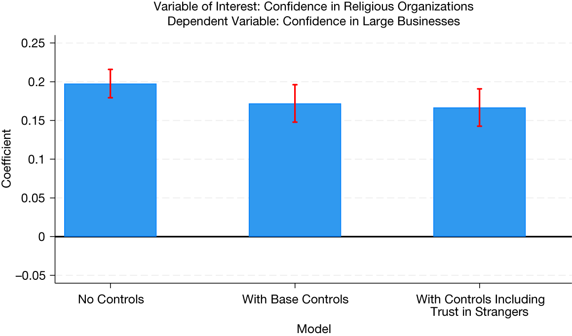


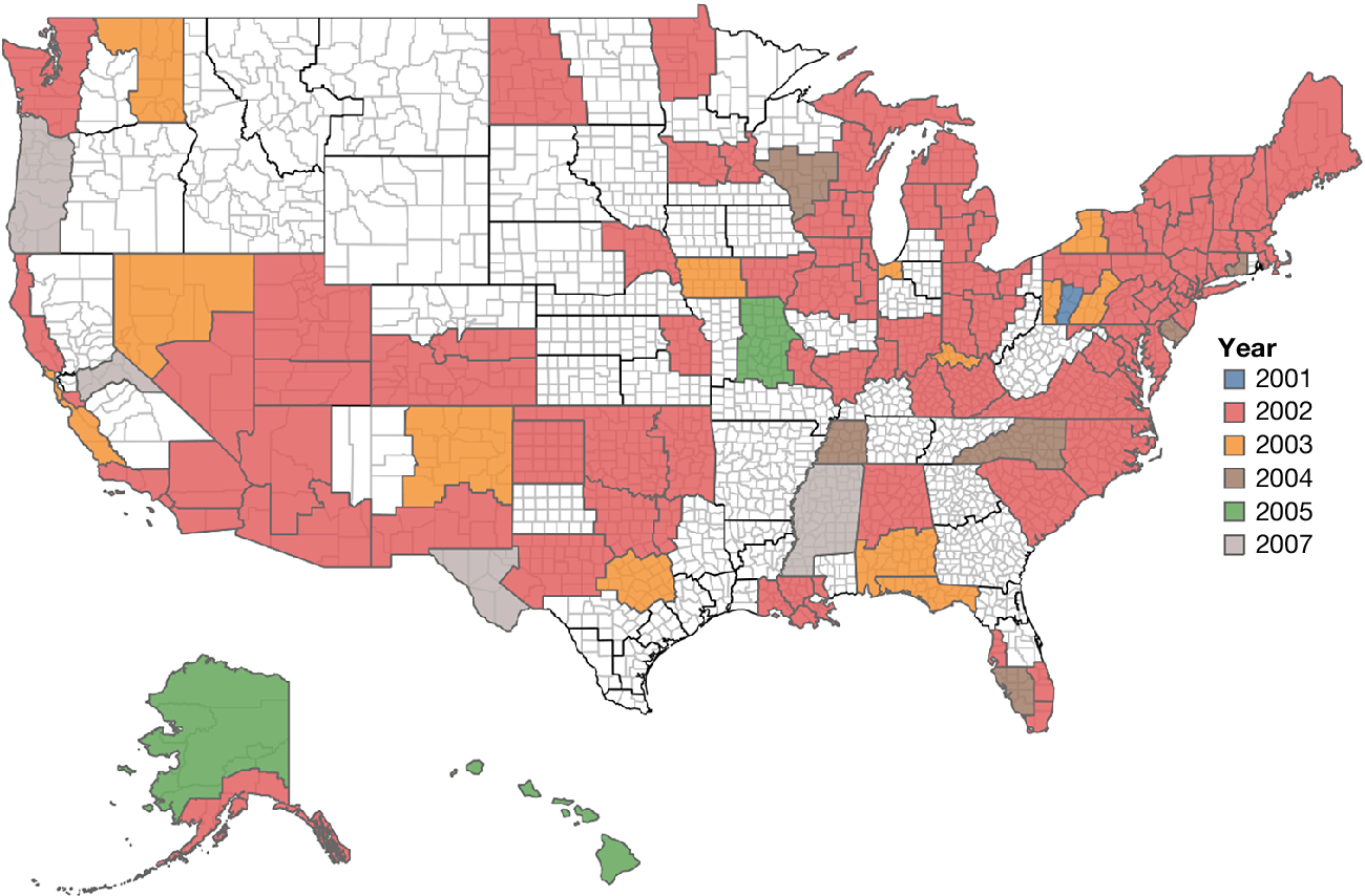
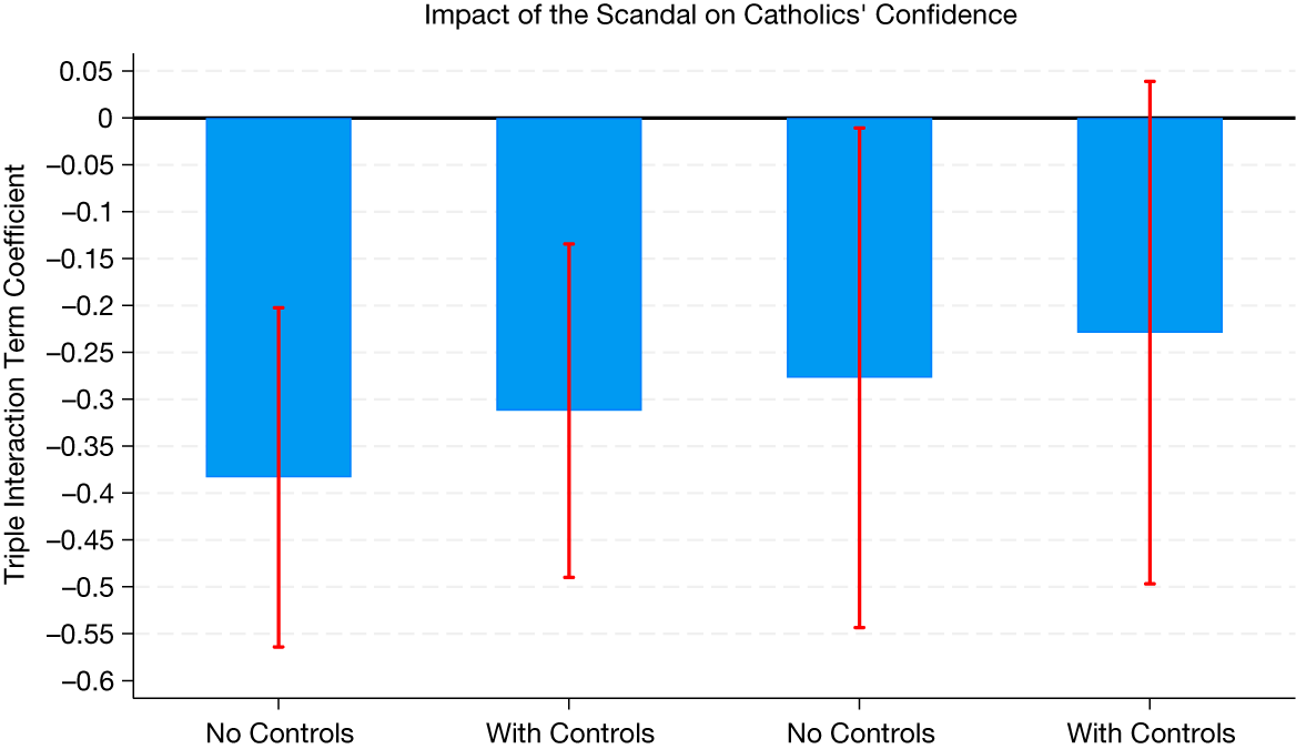


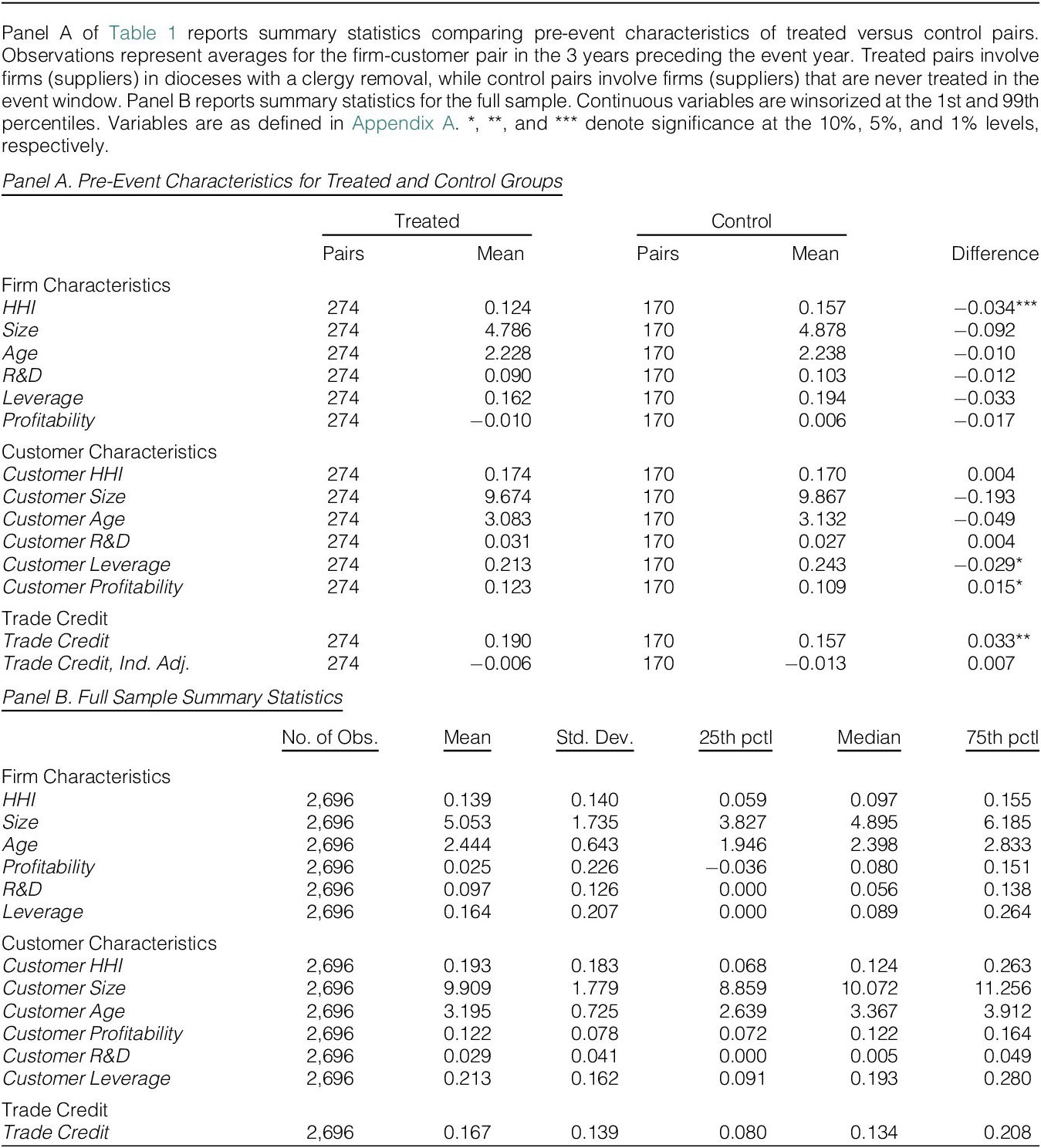
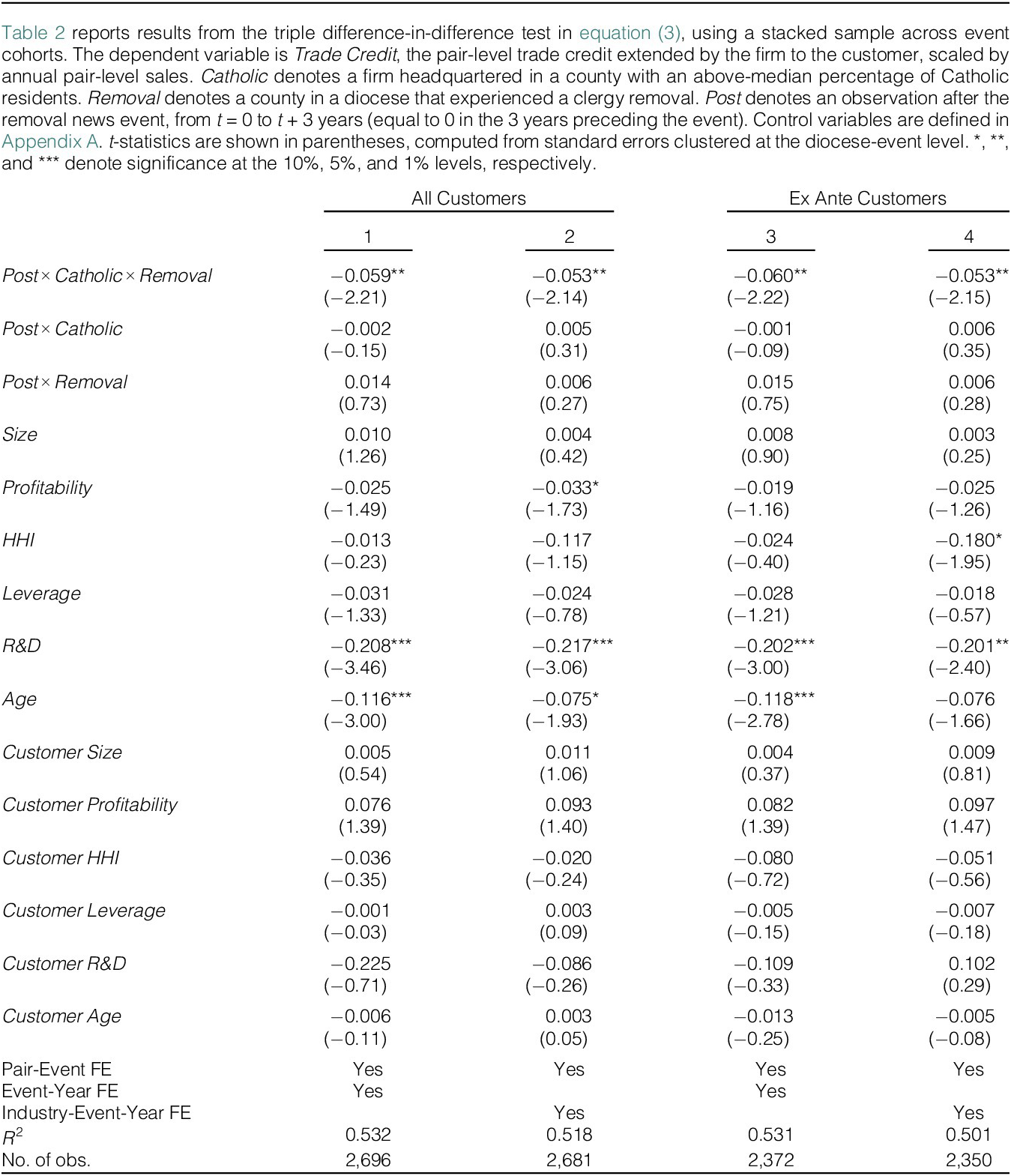
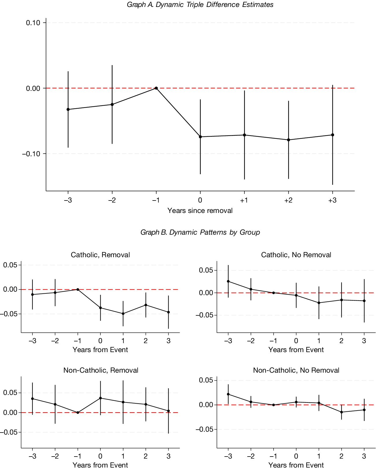
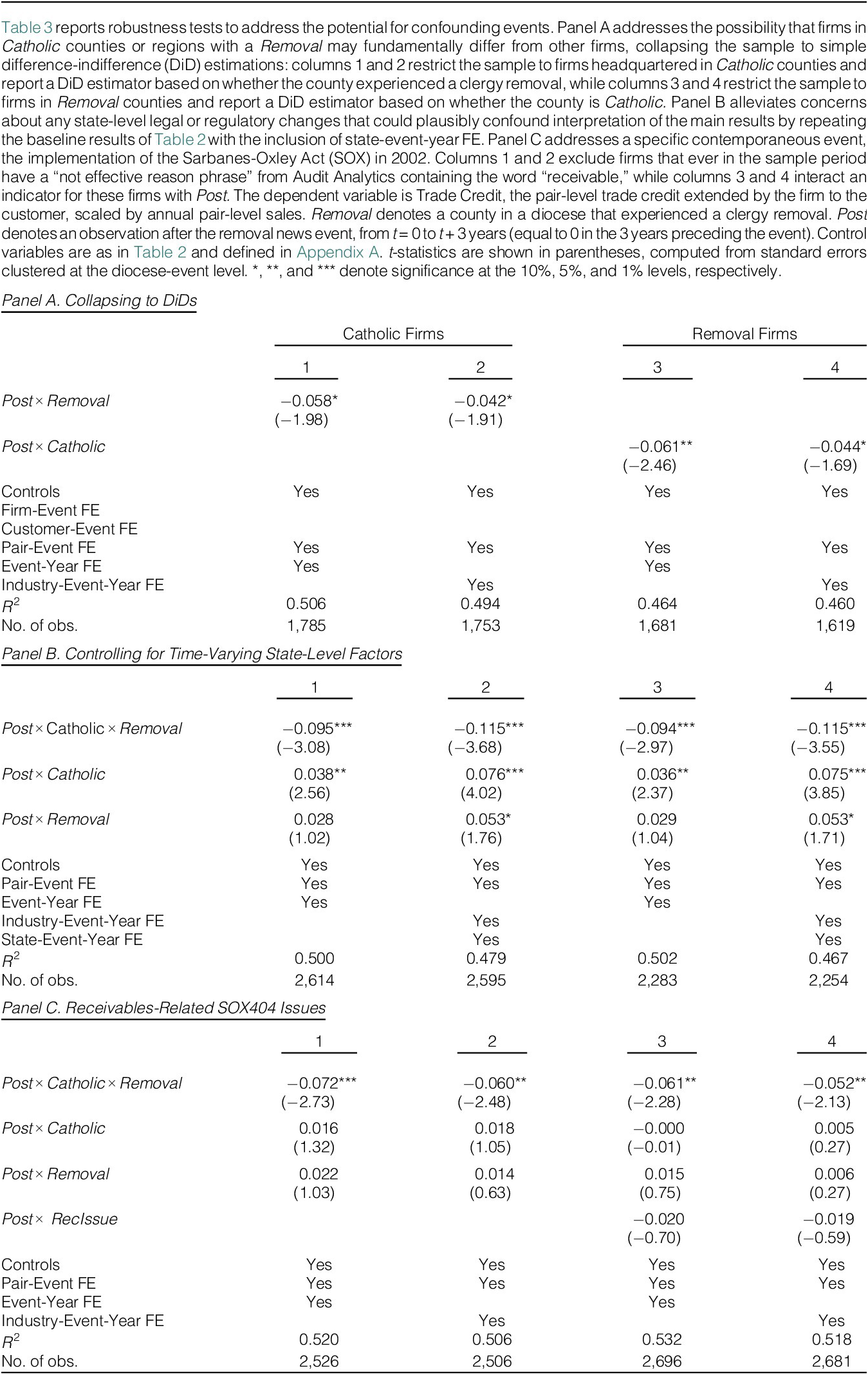
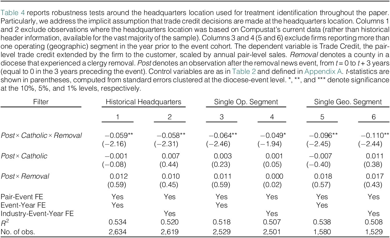
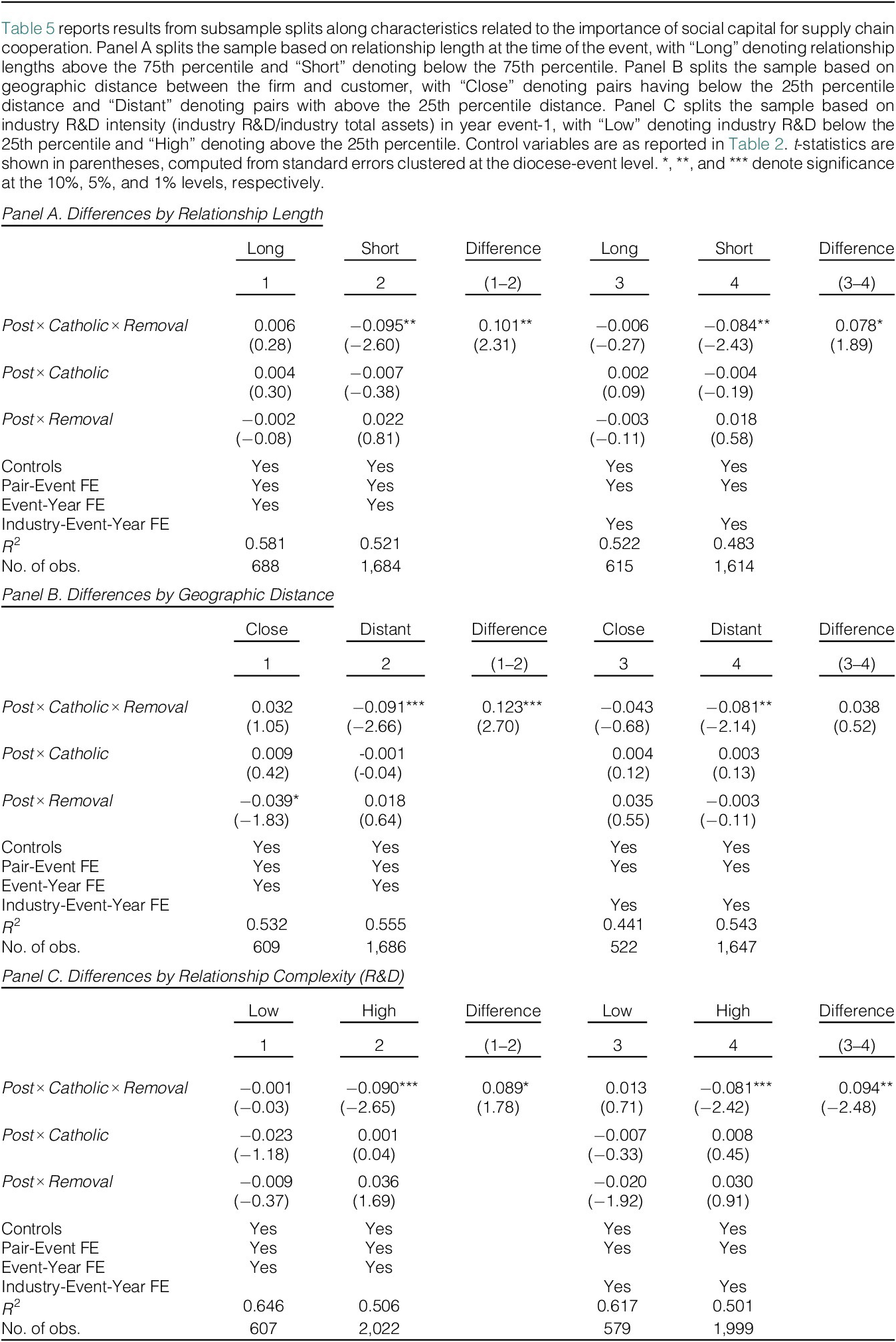
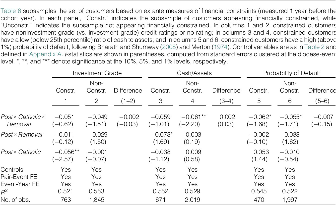
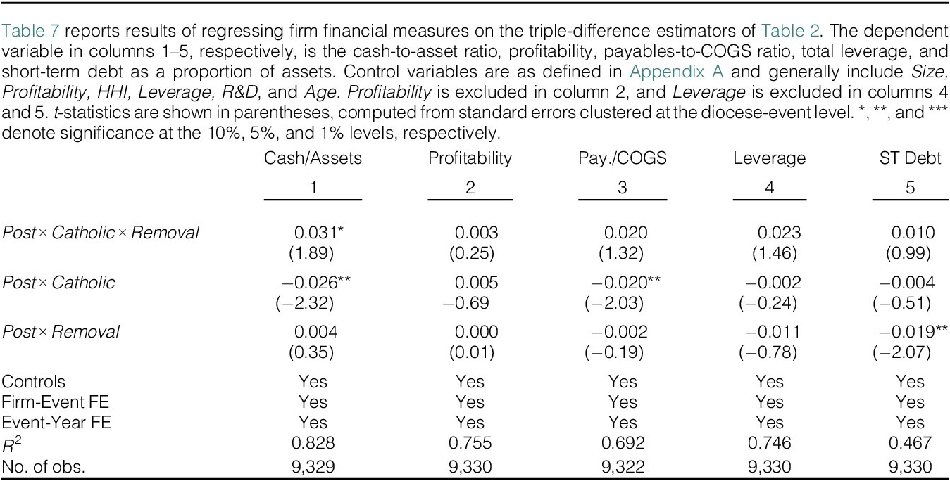
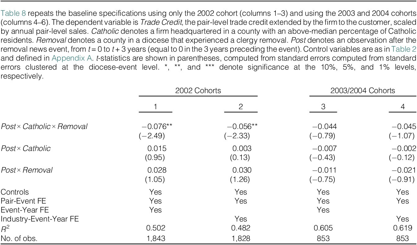
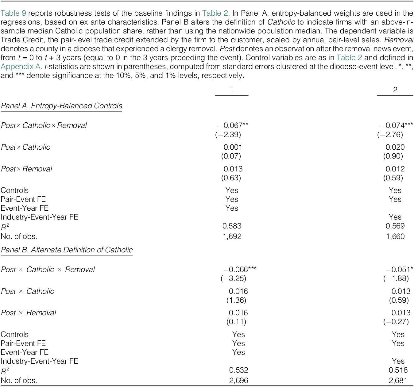
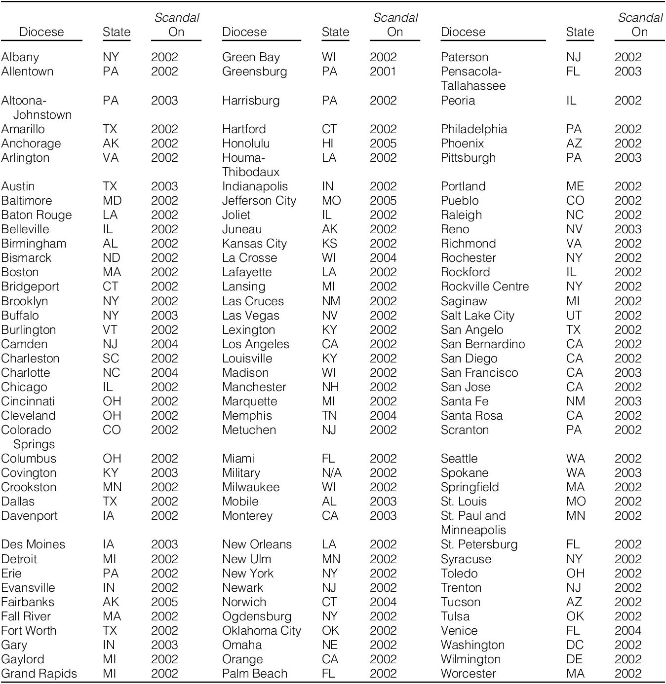
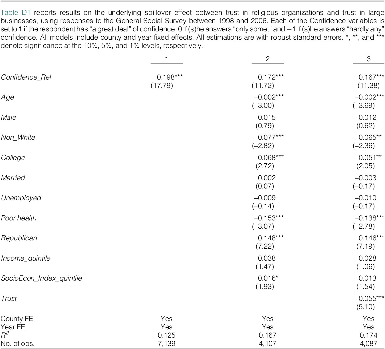
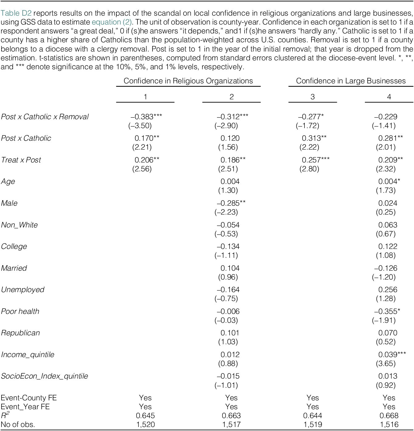
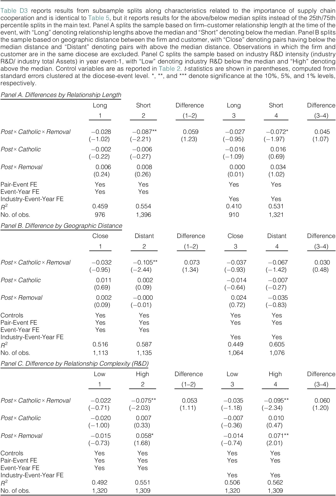
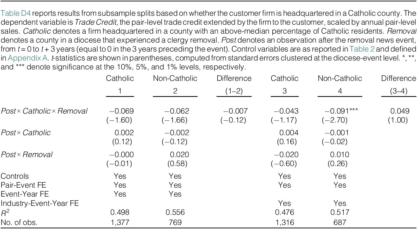
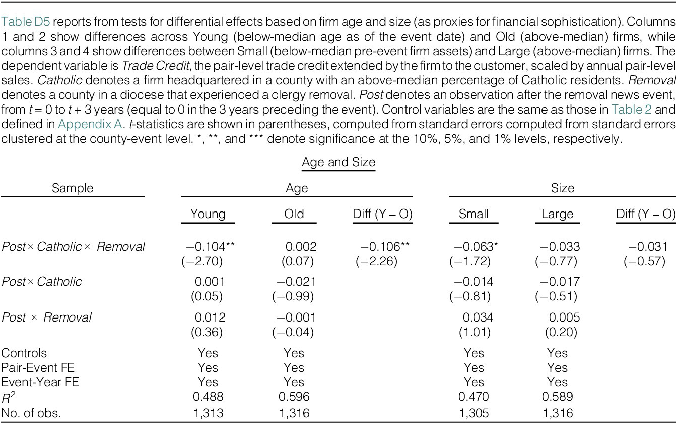
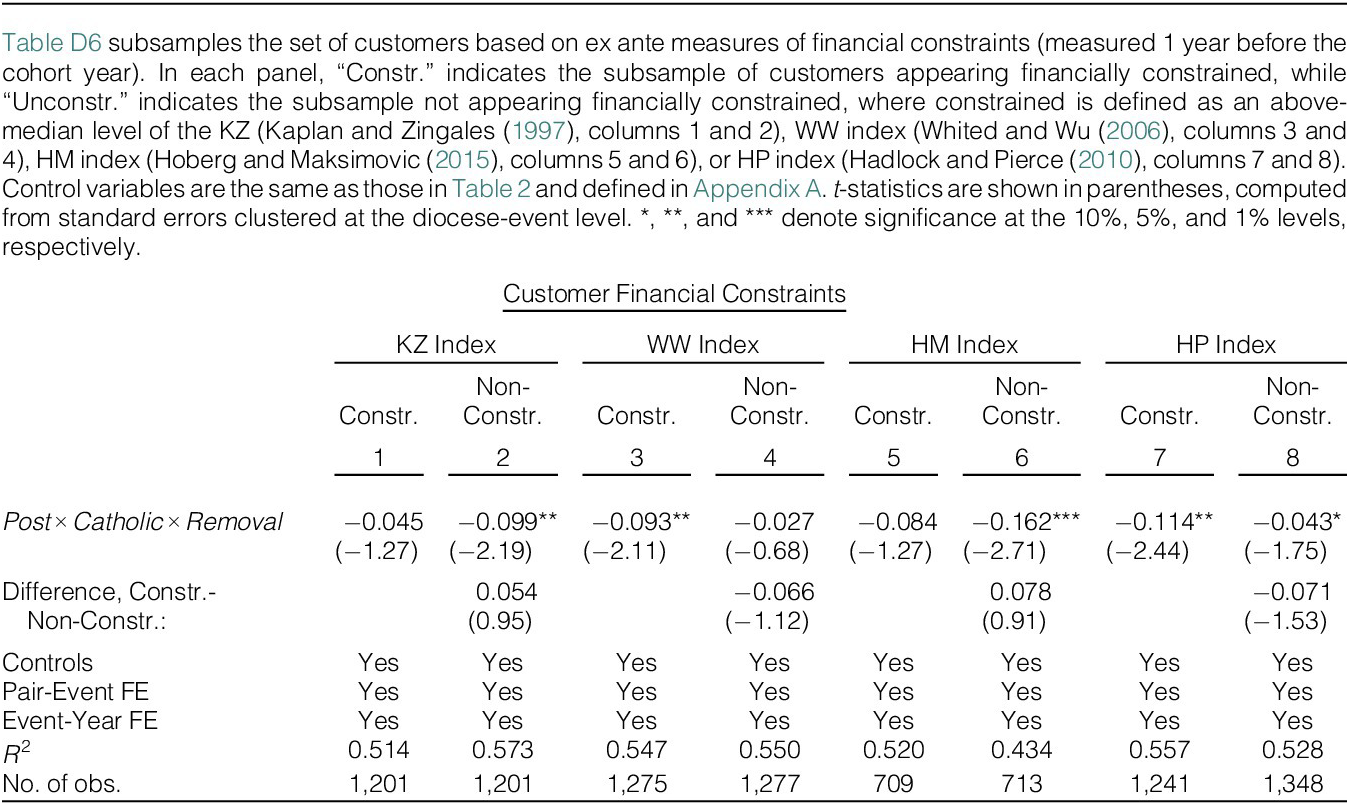

 Open access

