II. PSEUDOPOTENTIALS

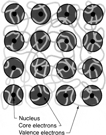
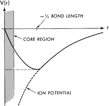
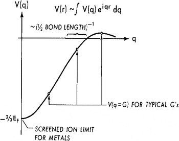
In the 1930s, Fermi,Reference Fermi⁴ Hellmann,Reference Hellman⁵ and others explored the construction of a pseudopotential to give the electron–ion interaction. Over the years, many forms have been introduced and used with success. If one adopts a model of a crystal as a periodic array of pseudoatoms or cores surrounded by a gas of valence electrons as shown in Fig. 1, then in the case of the EPM, all that is needed is an average potential to reproduce the optical data. In the 1950s, Phillips and KleinmanReference Phillips and Kleinman⁶ showed that because the Pauli principle forced valence electrons to stay out of the regions where the core electrons are, this could be represented by a repulsive potential in this region that would cancel part of the attractive potential of the ionic core and produce a weak pseudopotential. A typical pseudopotential V(r) for an ion is shown in Fig. 2. Assuming Fermi–Thomas screening by free electrons, the Fourier transform of V(r), V(q) is shown in Fig. 3. For electronic band structure calculations, we only need the values of V(q = G), where G is a reciprocal lattice vector. This is shown in Fig. 3.

FIG. 1.

Pseudopotential model with cores in a sea of valence electrons.

FIG. 2.

Schematic drawing of a real space pseudopotential.

FIG. 3.

Schematic drawing of a pseudopotential in reciprocal space.

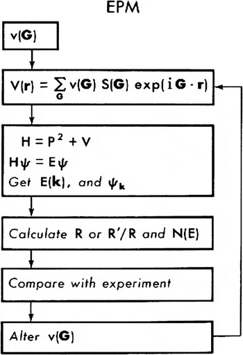
For systems like diamond, Si, and Ge in the diamond structure, only the first three G values for V(G) need to be considered. Hence by fitting just three Fourier coefficients or form factors, it is possible to get a band structure E(k) which is in agreement with the experimental data to within a few tenths of an electron volt over a range of a Rydberg. Not only were the energy levels accurate, the electronic density obtained by squaring the pseudo wave function gave a successful prediction of the x-ray results measuring the valence electron density.Reference Cohen and Chelikowsky¹ So the EPM approach shown in Fig. 4 was highly successful in interpreting many properties of semiconductors and explained the optical properties as explained earlier.

FIG. 4.

Block diagram illustrating the empirical pseudopotential method (EPM) approach.

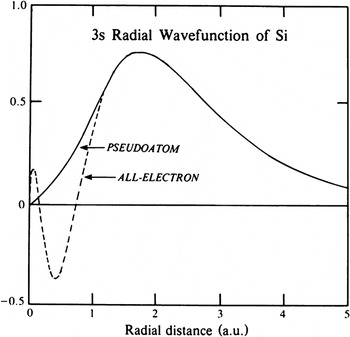
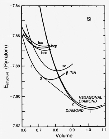
The next advance was to create the potentials from first principles using only the atomic number as input. This was achieved in several ways. The usual approach was to construct a potential which gave the same results as that obtained for an all-electron atomic calculation, but with a smooth nodeless tail in the core regionReference Hamann, Schluter and Chiang^7–Reference Vanderbilt⁹ as shown in Fig. 5. With this potential to express the electron–core interaction, the Coulomb core–core interaction, the Hartree mean field electron–electron interaction, and the electronic exchange–correlation contribution calculated using density functional theory within the local-density approximation (LDA),Reference Kohn and Sham¹⁰ it was possible to calculate the total energy of a solid for a specific crystal structure.Reference Ihm, Zunger and Cohen^11, Reference Cohen¹² This was first applied to study high-pressure phases of Si and Ge.Reference Yin and Cohen¹³ The energy versus volume E(V) for Si calculated using this method is given in Fig. 6.

FIG. 5.

The construction of an ab initio pseudopotential.

FIG. 6.

Calculated total energies as a function of volume for several structures of silicon.

The lattice constants, bulk moduli, and transition volumes and pressures are obtained in these studies. Several of the high-pressure phases of Si were predicted using this approach. By inputting the atomic masses, this total energy approach could be used to calculate phonon spectra and electron–phonon interaction parameters. Hence, many properties of solids could be calculated with only the crystal structure and the atomic numbers and masses as input. The use of the supercell conceptReference Cohen, Schlüter, Chelikowsky and Louie¹⁴ made it possible to deal with complex structures and multiatom systems. It is interesting to note that once the inner workings of the ab initio and EPM are understood, then semiempirical theories can be developed for calculating specific properties. An example is that, it can be shown that the bulk modulus for group IV, III-V, II-VI diamond and zincblende semiconductors is proportional to the bond length to the −3.5 power. Using relationship and a single ionicity parameter for the III-V’s and double that parameter for all the II-VI semiconductors, it is possible to obtain accuracy of less than 2% for these materials.Reference Cohen^15, Reference Cohen¹⁶

Despite the success of the above approach for calculating ground state properties, because the LDA does not give excited state (quasiparticle states) accurately, usually band gaps are underestimated. Hence unlike the EPM, this ab initio method could not give optical spectra in agreement with experiment. Two major improvements in recent years have been based on many-body theory. The first is called the GW approachReference Hybertsen and Louie¹⁷ which is used to obtain quasiparticle energies, and the second involves the use of the Bethe–Salpeter equationReference Rohlfing and Louie¹⁸ to compute the effects arising from the interaction between an electron and a hole produced in an optical transition. With these modifications, band gaps and optical spectra can be computed from first principles.

III. PHOTOVOLTAICS AND WAVE FUNCTION ENGINEERING

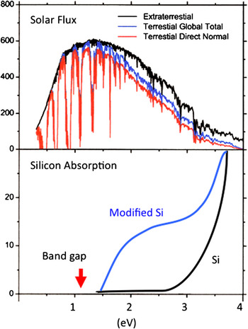
Silicon has been the prototype material for application in photovoltaic devices. Despite the fact that the absorption spectra of other materials can match the solar spectrum more effectively, the well-developed processing techniques and other properties of Si make it a very desirable material for this application. The purpose of this study is to explore the possibility of improving Si so that a better match with the solar flux of photons can be attained using a modified Si material (see Fig. 7). One way to modify Si is to use alloying or doping; another is to consider another structural phase induced by pressure and stabilized at atmospheric pressure. Here, we consider the latter case and focus on the structural phase called the R8 or Si XII phase. This phase can be made by using pressure on the diamond structure phase to induce a transformation to the metallic gray tin phase, and then release the pressure to produce the R8 phase.¹⁹

FIG. 7.

Schematic drawing of the comparison of the absorption spectrum of silicon and modified silicon with the solar spectrum.

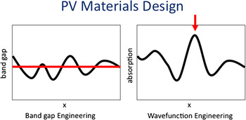
The concept and application of “band gap engineering” proposes that a property of a semiconductor is changed to change its band gap. The most popular example is alloying. The EPM was used to show how alloying various semiconductors would change the gaps and hence their optical responses. This concept is illustrated in Fig. 8, where the desired band gap is represented by a red line, and the changes in the semiconductor band gap by changing a parameter, such as alloy concentration, is represented by x. A possible problem for photovoltaic applications of this approach is that even if the band gap is optimized, the absorption may not be. For example, for Si, several proposals to change Si from an indirect gap material to a direct gap semiconductor suggest moving the minimum conduction band state usually located near the X point of the Brillouin zone to the center of the zone directly above the valence band state. Although this can be achieved, the matrix element for optical transitions does not change much. Calculations show that the wave function corresponding to the conduction band state “remembers” its form after the artificial movement of the k-point of this state. The top valence band state in Si is p-like and it puts electron density in the covalent bond. The minimum conduction band state puts electronic density (if occupied) in the interstitial region and the resulting dipole matrix element between these states is small.

FIG. 8.

Schematic drawing illustrating the band gap engineering and wave function engineering approaches for finding suitable photovoltaic materials.

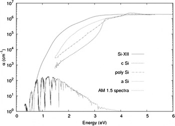
What is needed for photovoltaics is high optical absorption at the desired frequency, and this requires that attention be given to the wave functions of the states involved in the absorption process. Schematically, in Fig. 8, this motivation is illustrated by changing the variable x to give a peak (indicated by the red arrow) in absorption at the desired frequency. This is what is achieved in the schematic drawing for modified Si in Fig. 7. The results for the calculations for R8 (Si XII) are shown in Fig. 9 along with measured results for Si in the diamond structure (c-Si), polycrystalline and amorphous (alpha) Si. This plot clearly shows the increased absorption for R8 near the solar spectrum peak.

FIG. 9.

Comparison of the absorption spectrum of some structural forms of silicon with the solar spectrum.

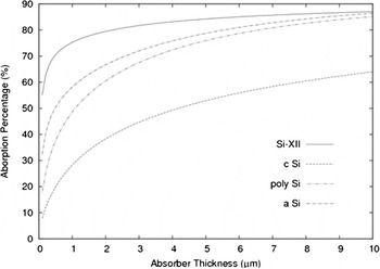
Although a very thick sample will absorb equally for all the above cases, it is desirable to have a sample as thin as possible. If we compute the energy absorbed W as a function of the thickness L for a solar intensity I(E) for samples of different absorption coefficients α(E), we have the expression

By solving this equation for the Si modifications shown in Fig. 9, we have determined the absorption percentage as a function of absorber thickness. As shown in Fig. 10, Si XII can be made thin and absorb as much as much thicker samples of Si in the other modifications. Current research on this material, both experimentalReference Ruffell, Sears, Knights, Bradby and Williams²⁰ and theoretical, is very encouraging. However, even if this modification of Si is not the best choice, this direction of research and development may hold promise for creating better voltaics through wave function engineering.

FIG. 10.

Absorption percentage of the solar flux versus absorber thickness for some structural forms of silicon.

IV. BORON NITRIDE NANOTUBES

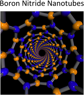
As in the case of the study of the optical properties of semiconductors, the study of boron nitride nanotubes (BNNTs) is another example of how theoretical and experimental research leads to the development of new understandings of nanostructures. Although most studies of nanostructures have focused on carbon materials, novel structures of this kind are not limited to carbon. For BNNTs, one can think of the hexagonal boron nitride (h-BN) sheet as the building block in analogy to graphene for a carbon nanotube (CNT). A rolled up sheet of h-BN is shown in Fig. 11. In fact, many of the interesting properties of h-BN are found in BNNTs, including large electronic band gap, strikingly white color, thermal stability to extreme temperatures in oxidizing environments, and neutron radiation absorption and shielding.

FIG. 11.

Ball and stick model of the structure of a boron nitride nanotube (BNNT).

The possible existence of BNNTs was predicted by theory,Reference Rubio, Corkill and Cohen²¹ and they were synthesizedReference Chopra, Luyken, Cherrey, Crespi, Cohen, Louie and Zettl²² soon afterward. The successes related to the prediction of the existence of these systems and some of their properties gave further credibility to the idea that the calculation techniques discussed above for bulk solids can be used for nanoscale objects. Until recently, because of the difficulties associated with producing large quantities of BNNTs, studies of these systems have been limited. Fortunately, new growth techniquesReference Smith, Jordan, Park, Kim, Lillehei, Crooks and Harrison²³ are yielding larger quantities and research and applications are increasing.

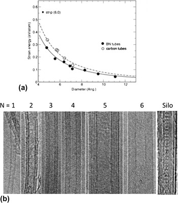
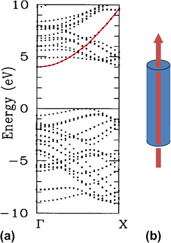
BNNTs are, relative to their planar parent, more stable than CNTs [see Fig. 12(a)], and when they are produced, it is difficult to destroy them. They can be multiwalled like CNTs. Figure 12(b) shows transmission electron microscope images of various BNNTs with wall number N ranging from 1 to 6. In addition, a so-called “silo” tube is shown. This is a multiwalled tube containing C60 molecules. Compared with CNTs, the electronic properties of BNNTs are relatively insensitive to geometrical variations. In fact, the BNNTs in the first six panels of Fig. 12(b) have similar semiconducting electronic structure. This means that the difficult job of separating semiconducting and metallic nanotubes, which is necessary for CNTs, can be avoided. In addition to pseudopotential total energy methods within the LDA and quasiparticle extensions of pseudopotential theory, tight binding models were used to study and predict the structural and electronic properties of BNNTs. The polar nature of the boron nitride bond led to the theoretical prediction that, in contrast to CNTs, BNNTs would, as mentioned above, be semiconductors irrespective of their differing diameters and chiralities.Reference Blasé, Rubio, Louie and Cohen²⁴ The calculated band gap, in the range of 5 eV, is consistent with optics studies. A plot of the band structure E(k) is shown in Fig. 13(a) using the LDA. Hence, the band gap for this calculation is underestimated. The calculations predict that with doping, either within the tube wall or via functionalization, the electronic properties can be changed considerably. As an example, the electronic structure associated with the lowest conduction band of BNNTs is interesting because if the tube is doped n-type to occupy this state, the electronic charge resides inside the tube, not on it, with a maximum value of the charge density occurring about 2 Å in from the wall of the tube. Hence these n-doped tubes should act like pipes filled with “free” electrons as shown schematically in Fig. 13(b). In addition, BNNTs have been shownReference Cumings and Zettl²⁵ to be excellent electron field emission sources, with emission turn-on voltages comparable to those for CNTs. In contrast to CNT field emitters, BNNT field emitters display extremely stable field emission currents.

FIG. 12.

(a) Calculated strain energy versus radius showing the relative stability of BNNT and carbon nanotube. (b) Electron microscopy of multiwalled BNNTs and a silo BNNT containing C60 molecules.

FIG. 13.

(a) The electronic band structure of a BNNT. (b) Schematic drawing illustrating the charge density associated with electrons in the lowest conduction band for a doped BNNT.

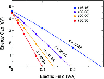
An interesting theoretical prediction is that the band gaps of BNNTs can be externally tuned.Reference Khoo, Mazzoni and Louie²⁶ The minimum band gap of BNNTs can be reduced with sufficiently strong electric fields. This “giant Stark effect” is analogous to the conventional Stark effect for atomic orbitals. The mixing of electronic states in BNNTs in transverse electric fields is enhanced because of the field-induced splitting of the electronic bands with states having their electron and hole densities on opposite sides of the BNNT. The reduced screening, because of the insulating behavior, allows a significant difference in the electric potential seen at the two sides of the tube. Hence states that in the absence of a field would be degenerate with similar wave functions at opposite sides of a tube are now split. The effect depends on tube diameter as shown in Fig. 14. There is experimental confirmation for this effect.Reference Ishigami, Sau, Aloni, Cohen and Zettl²⁷

FIG. 14.

Calculate dependence of the band gap as a function of the strength of an applied electric field transverse to a BNNT.

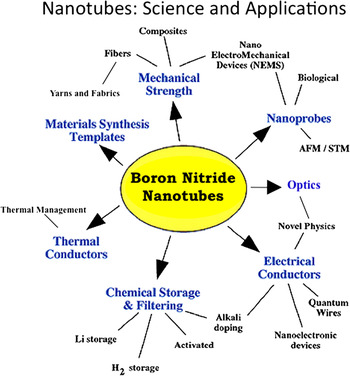
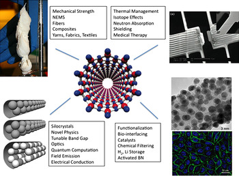
Because of their novel properties, the study of BNNTs may provide an opportunity to study novel physical phenomena and applications.Reference Cohen and Zettl²⁸ Some possibilities are shown in Figs. 15 and 16.

FIG. 15.

Chart of applications and properties of BNNTs.

FIG. 16.

Examples of applications and properties for functionalized BNNTs.

V. SUPERCONDUCTIVITY IN MODIFIED SEMICONDUCTORS AND INSULATORS

It has been 100 years since the discovery of superconductivity in Hg.Reference Onnes²⁹ The theory explaining this discovery came 46 years later with the seminal work of Bardeen, Cooper, and Schrieffer (BCS),Reference Bardeen, Cooper and Schrieffer³⁰ which completely explained the properties of superconductors discovered up to that time. A major early goal was to find superconductors with high transition temperatures. However, the maximum transition temperature for superconductors increased on an average of only 1 °C every 3 years until the late 1980s when superconductivity was discovered in materials based on copper and oxygen.Reference Bednorz and Muller³¹ The highest transition temperature observed in systems of this type is around 165 K,Reference Gao, Xue, Chen, Xiong, Meng, Ramirez and Chu³² and that is the current record.

After the original discovery of superconductivity, many materials were tested. It was quickly found that only metals exhibited superconductivity, so having conduction electrons is crucial. Semiconductors and insulators are therefore not expected to exhibit superconducting properties unless they are doped or modified in other ways to make them conduct at low temperatures. In the 1960s, the possibility of superconductivity in degenerately doped semiconductors using model systemsReference Cohen^33, Reference Cohen and Parks³⁴ motivated experimental searches, and within a short time, superconductivity was found in GeTe,Reference Cohen and Parks³⁴ SnTe,Reference Cohen and Parks³⁴ and SrTiO₃.Reference Schooley, Hosler and Cohen³⁵ These were all doped low carrier density systems, and the transition temperatures were below 1 K. Since this early work, more low carrier density superconductors have been found.

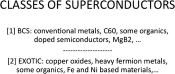
It is useful to separate superconducting materials into two classes 1 and 2 as shown in Fig. 17 to discuss the role that theory has played in explaining and predicting properties and even the existence of new superconductors. Class 1 contains “conventional BCS superconductors” like Al, Sn, Pb, Hg, etc. For these materials there are many experimental tests showing that the BCS theory is applicable. The same can be said for the other members of this class, such as degenerate semiconductors. The BCS theoretical description of their superconducting properties based on electron pairing induced by electron–phonon coupling works extremely well, and it is possible to use the theory to predict new superconductors. In this article, we will restrict ourselves to class 1 materials, since for class 2, as mentioned above, there is no consensus at this time regarding the correct theory to explain their properties. For class 1, it is generally accepted that all experimental data have been explained. In some applications of the theory, such as the calculation of T _c, the precision needed has not been achieved in general. However, this shortcoming is usually attributed to our inability to calculate the needed input to the BCS theory, i.e., the normal state properties, with sufficient precision.

FIG. 17.

Classes of superconductors.

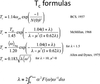
What about the highest T _c’s? The current upper limit record for class 1 is around 40 K for MgB₂. Although this is significantly lower than for materials in class 2, it is still difficult to predict whether the next record breaking T _c will be for a material in class 1 or class 2. The advantage of studying this problem for class 1 is that the theory is well established and to a great extent understood for some materials systems, hence possible paths to higher T _c values can be explored. Just after the publications of the BCS theory, the most commonly used expression for calculating T _c was the BCS expression listed in Fig. 18. This formula for T _c is based on “the BCS Model” which assumed a weak coupling pairing interaction N(0)V, where V is the net attractive pairing potential and N(0) is the density of states at the Fermi energy. The exponential dependence of T _c on N(0) is the reason for the strong focus on this quantity for increasing T _c. The interaction V is composed of an attractive phonon component and the repulsive Coulomb potential. These compete as seen in the following formula for the transition temperature T _c based on the BCS model

FIG. 18.

Formulas for calculating the superconducting transition temperature.

Here, E(phonon) represents an average energy of the phonons such as the Debye temperature, and the net interaction in the exponent is the dimensionless phonon pairing interaction λ and the modified repulsive electron–electron interaction μ*. These are the two components of N(0)V, i.e., N(0)V can be viewed as λ − μ*. Superconductivity is expected when this difference is positive. The Coulomb interaction is modified (hence the asterisk superscript) because of the difference in energy scales between the two pairing potentials.

McMillanReference McMillan³⁶ included the effects of renormalization and of stronger coupling when the electron–phonon parameter λ became larger. This equation (Fig. 18) can be used for values of λ up to about 1.25. The McMillan equation became the T _c equation of choice, and it is still used. However, applications beyond the above limit led to incorrect estimates of the maximum transition temperature. This gave a pessimistic view since the resulting expression for T _c(λ) for the McMillan equation saturates. Later, Allen and DynesReference Allen and Dynes³⁷ (Fig. 18) solved the EliashbergReference Eliashberg³⁸ equations for several model phonon spectra and found that, for large λ, T _c was proportional to λ ^1/2 (Fig. 18) with no saturation.

Modern calculations of T _c are usually done by solving the Eliashberg equations numerically. This approach gives precise estimates when precise normal state properties are used as input. There are model solutions that result in simple formulas (for μ = 0) such as the Kresin–Barbee–Cohen modelReference Kresin^39, Reference Bourne, Zettl, Barbee and Cohen⁴⁰ based on a flat phonon spectrum,

where <ω ²> is an appropriately averaged square of the phonon frequency. This expression gives the correct λ ^1/2 limit at high λ and the exponential BCS model solution for small λ.

Because of these developments, the shift in searching for higher T _c changed from a search for large N(0) materials to looking for large λ’s. The separation into N and V suggested by the NV parameter is not appropriate for most materials since most systems are not modeled well by the BCS model solution. When considering the shift from looking for large N(0) to large λ’s, an important caveat to add is that strong electron–phonon interactions often lead to structural instabilities. Hence, when considering large λ’s, an important caveat is that strong electron–phonon interactions often lead to structural instabilities as described earlier. Therefore, the desired material may not be stable at atmospheric pressure.

As discussed above, successes using ab initio calculations came with the development of the Eliashberg theory and the advances made in calculating normal state properties. To illustrate some of the features of this approach for phonon-mediated pairing, an expression for calculating λ is given in Fig. 18 in terms of the Eliashberg spectral function which can be viewed as the product of the electron–phonon coupling times the phonon density of states,

where N is the density of states per spin at the Fermi level, g_{kk ′} is the electron–phonon matrix element, and is the frequency of the phonon. It is often convenient to solve the Eliashberg equations in the Matsubara representation where

Here, the conventional λ is represented by the average

The first ab initio calculations for semiconductor-based systems were for high-pressure phases of Si.Reference Chang, Dacorogna, Cohen, Mignot, Chouteau and Martinez⁴¹ These calculations dealt with the averaged values for the input to the Eliashberg equations, and the approach used a method that had just been developed for calculating electron–phonon couplings. The application to high-pressure Si was a dramatic example of the power of this approach. Using only the atomic number and atomic mass for Si, the total energies for candidate crystal structures were compared at various pressures. Several new forms of Si were successfully predicted. Two of these, simple (or primitive) hexagonal and hexagonal close-packed Si were studied in detail. The existence of these phases, their stability, lattice constants, mechanical properties, electronic structures, vibrational properties, and electron–phonon coupling were then determined from first-principles calculations. The Coulomb potential μ* could be estimated using the densities of states at the Fermi energy as a scaling parameter. The result was a successful prediction of superconductivity for both phases and an estimate of T _c and its pressure dependence. Considering the limited input and the accurate predictions, it could be said that high-pressure Si became the best-understood superconductor.

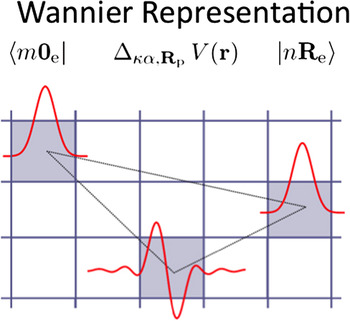
As mentioned earlier, the quest for higher superconducting transition temperatures began in 1911, and although our theoretical understanding of superconductivity has advanced considerably and successful predictions of new superconductors have been made for class 1 superconductors, we still do not have a consensus on a well-defined path for increasing T _c. Fortunately, for strong electron–phonon coupling, the Allen–Dynes limit, which does not saturate, is more optimistic than the McMillan equation, which saturates as the coupling gets stronger. The search for larger electron–phonon couplings also depends on the development of methods capable of calculating the couplings with high precision. The early approach for high-pressure Si was developed to work with a plane wave basis set,Reference Chang, Dacorogna, Cohen, Mignot, Chouteau and Martinez⁴¹ and calculations at many points in reciprocal space were needed to obtain a good estimate of λ. A recent development that has many advantages is based on the use of Wannier functions to evaluate electron–phonon couplings.Reference Giustino, Cohen and Louie⁴² This real space approach is illustrated schematically in Fig. 19 where an electron in one cell is coupled to an electron in another cell via a vibrating atom in a third cell. A typical calculation using this approach can be equivalent to plane wave calculations that would require millions of points in reciprocal space for convergence. In the area we are considering, semiconductors and insulators, we note that applicationsReference Giustino, Cohen and Louie⁴² have been made to explore superconductivity in doped diamond and SiC.Reference Giustino, Cohen and Louie^42–Reference Noffsinger, Giustino, Louie and Cohen⁴⁴

FIG. 19.

Schematic drawing showing the Wannier approach for calculating the interaction between two electrons (in rows 1 and 2) via an atomic vibration (in row 3).

Searching for higher T _c materials has become a search for conditions that will lead to large λ’s either via large densities of states or through large electron–phonon pairing potentials. An interesting alternative viewReference Moussa and Cohen⁴⁵ is to express λ as a dimensionless ratio of electronic and vibrational spring constants

where <I ²> is the square of the displacement-induced electron scattering matrix element averaged over the Fermi surface, <ω ²> is an average of the square of the phonon frequencies, and N(E_F) is the electronic density of states at the Fermi energy. For harmonic systems, the M <ω ²> and λ are roughly independent of M. Perhaps a better view is to look at T _c for large coupling where

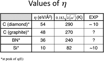
This equation implies that what is needed for higher T _c’s is stronger electronic spring constants and light masses. This can be extended to explore compounds with multiple masses in a unit cell, and estimates can be made using information from molecular fragments.Reference Moussa and Cohen⁴⁶ We note that strong electronic spring constants are expected for strong bonds such as the covalent bonds in diamond. The challenge in the latter case is getting enough mobile carriers. If one considers the energy dependence of the electronic spring constant, then a possible path to higher T _c is to dope into peaks in the energy-dependent electronic spring constant. A theoretical estimateReference Moussa and Cohen⁴⁵ suggests that very high transition temperatures are possible as shown in Fig. 20. Some success has been reported for experiment,Reference Ekimov, Sidorov, Bauer, Mel’nik, Curro, Thompson and Stishov⁴⁷ but the T _c level is still not very high.

FIG. 20.

The peak values of the electron spring constant and the associated transition temperatures (calculated and measured values) for some materials.

It is not clear whether class 1 or class 2 type materials are more promising in the search for higher T _c’s. The known materials of class 2 have the highest T _c’s, but without a descriptive theory, it is difficult to make quantitative predictions. For class 1, it is suggested here that materials with strong bonds and light masses should be studied further. Hence modified semiconductors and insulators appear promising candidates. An encouraging sign is that the transition temperature is expected to increase with the electron–phonon coupling for large values of the coupling. A caveat is that large electron–lattice coupling can result in structural transitions. A possible remedy for this is to choose systems where the integrity of the crystal structure is determined by different bonds than those that couple strongly to the superconducting electrons. This is the case for MgB₂.