INTRODUCTION
Chrysogorgia is a relatively speciose genus, with 62 currently recognized species (Cairns, Reference Cairns2001, Reference Cairns2002, Reference Cairns2007). Presently, only nine species are known from the north-western Atlantic, all of which were described from environments associated with the continental slope and the lee of Caribbean islands, and from relatively shallow waters (over 40% of the observations reported in Cairns, Reference Cairns2001 have an average depth <500 m). Recently, a series of cruises on the New England and Corner Seamounts (north-western Atlantic) revealed a wealth of octocorals (Thoma et al., Reference Thoma, Pante, Brugler and France2009; Shank, Reference Shank2010), including chrysogorgiids (Watling, Reference Watling2007; Mosher & Watling, Reference Mosher and Watling2009; Thoma et al., Reference Thoma, Pante, Brugler and France2009), from much greater depths (for Chrysogorgia: 1533–3860 m). Among the specimens collected during these cruises, colonies of Chrysogorgia are of particular interest as they are large and are characterized by a sinistral spiral, a feature that until now was almost exclusively observed from Pacific specimens. In this paper we describe the material collected on the New England and Corner Seamounts based on genetic and morphological data, and discuss their affinities with previously described species from the Atlantic and Pacific Oceans.
Octocorals are relatively simple animals, with, in some groups, few characters available to taxonomists (e.g. McFadden et al., Reference McFadden, Sánchez and France2010). Unfortunately, recent comparative analyses revealed incongruence between several morphological traits (such as colony branching, polyp and sclerite morphology) and molecular phylogenetic information at multiple taxonomic levels (France, Reference France2007; Dueñas & Sánchez, Reference Dueñas and Sánchez2009; Pante & France, Reference Pante and France2010). These results imply that morphological variation does not necessarily reflect evolutionary history, and it is therefore prudent to combine morphological information with other lines of evidence when describing new octocoral taxa. In Chrysogorgia, as in many other octocoral groups, attention is focused on branching patterns as well as sclerite morphology and arrangement (e.g. Cairns, Reference Cairns2001). No statistical analysis has been conducted in this group to estimate the amount of intra-specific variability, or to validate the phylogenetic usefulness of these characters by comparing them with genetic data. Here, we present a multivariate analysis of the morphological variation among 23 Chrysogorgia colonies, and investigate the correlation between morphology and genetic variation at the mitochondrial locus msh1. We chose this marker because it may be the most variable mitochondrial gene in octocorals (France & Hoover Reference France and Hoover2001; Wirshing et al., Reference Wirshing, Messing, Douady, Reed, Stanhope and Shiuji2005; van der Ham et al., Reference van der Ham, Brugler and France2009; Herrera et al., Reference Herrera, Baco and Sánchez2010; McFadden et al., Reference McFadden, Benayahu, Pante, Thoma, Nevarez and France2011) and was useful in genetically distinguishing morphotypes of some deep-sea octocorals (e.g. France, Reference France2007).
Technological advances and the relative availability of remotely operated vehicles (ROVs) catalysed studies on the community ecology of deep, benthic ecosystems (e.g. Lundsten et al., Reference Lundsten, Barry, Cailliet, Clague, DeVogelaere and Geller2009; McClain et al., Reference McClain, Lundsten, Ream, Barry and DeVogelaere2009), and many research groups now use in situ video footage and photographs to make faunal inventories. In fact, the resolution of the video equipment on ROVs allows researchers to observe individual coral polyps on live colonies, and even see minute details such as pinnules on tentacles. Such capabilities have led researchers to try to identify octocorals colonies to the species level. In this paper we will discuss the limits of using these technologies to identify Chrysogorgia colonies.
MATERIALS AND METHODS
Collection and preservation
Most of the material described here was collected during three expeditions to the New England (NES) and Corner Seamounts (CS). The first two expeditions, conducted in 2003 and 2004, were named Mountains-in-the-Sea I and II, respectively, and the 2005 expedition named Deep Atlantic Stepping Stones. L. Watling was Chief Scientist on all three expeditions and can be contacted for details. Summaries of all expeditions can be found on the website of NOAA's Ocean Exploration Program (currently www.oceanexplorer.noaa.gov), and a map of the area with sampling locations can be found in Thoma et al. (Reference Thoma, Pante, Brugler and France2009). Specimens were obtained by use of the deep submergence vehicle (DSV) ‘Alvin’, in 2003 and the ROV ‘Hercules’, in 2004 and 2005. In all cases, specimens were collected by use of a manipulator equipped with a claw that could break (in the case of ‘Alvin’) or cut off (in the case of ‘Hercules’) pieces of large colonies, or remove entire small colonies from the substrate. All collected colonies or pieces of colonies were put in an insulated collection box on the vehicle for return to the research vessel. On-board, the specimens were kept in cold seawater until they could be fixed and preserved. After removal of colony pieces for genetic and reproductive studies (herein referred to as ‘isolates’), all specimens were fixed in a dilute formalin solution (4%) for 12 hours and then rinsed and stored in 70% ethanol. Specimens for molecular genetic analysis were preserved in 90–100% ethanol or frozen at –80°C. All specimens used for morphological analysis were deposited in the Yale Peabody Museum (YPM).
Microscopy
Polyps from preserved colonies were individually photographed using light microscopy, and one or more polyps per colony were examined for sclerite composition and morphology. Sclerites were dissolved from the surrounding polyp and branch tissue using household bleach. Following several washings in deionized water, individual sclerites from select specimens were mounted on standard scanning electron microscope stubs with blackened double-sided tape. Individual polyps to be examined with scanning electron microscope were removed from a branch, dehydrated to 100% ethanol, and dried using a Samdri Critical Point Dryer (except for the partially digested polyp of NAS201-2, Figure 7E, which was only air-dried). Digital images of sclerites and polyps were obtained using Hitachi S-800, S-3000N, and S-4800 scanning electron microscopes. Sclerite and polyp images were isolated from the original image background, and their contrast and brightness were adjusted in Adobe Photoshop. Images were otherwise unaltered in accordance with current scientific image processing guidelines.
Branching sequence
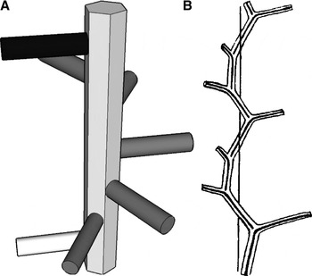
Branching sequence was determined for all colonies based on the following parameters: the direction of the spiral; the number of branches that one needs to travel up the stem to recover the plane of a reference branch; and the number of revolutions necessary to do so (Versluys, Reference Versluys1902; Cairns, Reference Cairns2001, Reference Cairns2002, Reference Cairns2007). Travelling up the stem from the base to the tip of the colony (i.e. direction of colony growth), the spiral can be clockwise (dextral, abbreviated R) or counter-clockwise (sinistral, abbreviated L). A three-dimensional model is presented in Figure 1 to explicitly show how to determine the branching sequence.
On the left: model representing the main stem and some branches of a hypothetical Chrysogorgia colony. To determine branching sequence, one counts the number of branches required to be in the same plane as a reference branch (white). In this example, the 6th branch (black) is in the same plane as the reference branch, and only one revolution is necessary to spiral back to the reference plane. Also, in this case the spiral is clockwise when looking upward (in the direction of colony growth). This hypothetical colony therefore has a 1/6R sequence. On the right: original (figure 21, p. 21 from Versluys, Reference Versluys1902), representing the branching sequence of a 1/3L spiral.

Measurements
Polyp height was measured from the base (on branch) to the mouth. Polyp width was measured at the neck (sensu Bayer et al., Reference Bayer, Grasshoff and Verseveldt1983: plate 2, p. 39). Measurements (e.g. colony height) were taken directly on the preserved colony when possible or from photographs using the program ImageJ (Rasband, Reference Rasband1997–2008; Abramoff et al., Reference Abramoff, Magelhaes and Ram2004) when measuring directly was not practical (e.g. measurement of angles). The orthostiche distance, defined by Versluys (Reference Versluys1902) as the distance separating aligned branches along the axial skeleton (and see Cairns, Reference Cairns2001), was determined using standard calipers. The angle between the stem and the branch was measured so that it is obtuse if the branches are oriented upwards. All measurements of sclerites were done from light microscope imagery using ImageJ. Measurements are reported as mean ± one standard deviation, range and sample size.
Genetic analysis
DNA was extracted from frozen (–80°C) or ethanol-preserved (95%) tissue using a modified CTAB protocol (France et al., Reference France, Rosel, Agenbroad, Mullineaux and Kocher1996) or using the MasterPure DNA purification kit (Epicenter). The first 697 base pairs (bp) of the protein-coding, mitochondrial msh1 gene were amplified and sequenced as described in Thoma et al. (Reference Thoma, Pante, Brugler and France2009). DNA sequences of specimens representing each haplotype, for each seamount peak, were submitted to GenBank. The phylogenetic relationship between the species presented here and other Chrysogorgia species will be presented in a forthcoming publication.
Statistical analysis
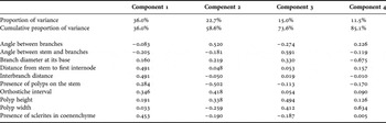
Variation in sclerite length across haplotypes and polyp body compartments was characterized using frequency histograms. The effect of growth on continuous variables related to colony morphology was assessed by plotting ordered measures (taken from the base to the tip of the colony) for the two specimens that were sampled with their holdfast (KEL407-2 and NAS201-2) and a third, tall colony (KEL619-1) that was sampled very close to its base. The interbranch distance is used as an example. Eight continuous and two discrete (presence/absence, coded as 0 and 1) variables were used in a principal components analysis (PCA; characters listed in Table 1). Measures from individual specimens were used, and continuous variables were summarized as means. Specimen LYM201-2 (YPM 38593, haplotype A) from Yakutat Seamount was removed from the analysis as the colony was highly damaged and all characters could not be scored with confidence. All statistical analyses and plotting were done in R (R Development Core Team, 2010).
Proportion of variance and loadings for the first four components of the principal components analysis.

RESULTS
Correspondence between msh1 haplotypes and morphotypes
Four msh1 haplotypes (A, B, C and E) were found among the 23 colonies sampled on the NES and CS. Haplotypes A and B differ by one base pair only. The mutation is unique to A among our samples, and appears to be the derived state, when compared to haplotypes B, C and E, the chrysogorgiid Radicipes gracilis (Verrill, 1884) (GenBank ID DQ297424) and the primnoid Narella dichotoma Versluys, 1906 (GenBank ID EF060048). Haplotypes C and E differ from A by 3 and 7 bp, respectively.
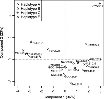
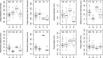
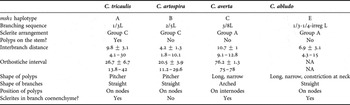
Groupings based on msh1 haplotypes were congruent with the morphological characters measured (Figures 2 & 3). The first two axes of the PCA explained 59% of the overall variance (component loadings: Table 1). Based on the ten characters used in the PCA, haplotypes A and B were most distinguishable from each other based on the presence/absence of polyps on the main stem, the presence/absence of sclerites in the branch coenenchyme, and distances between (1) branches on the stem and (2) stem and first branch internode. Haplotype E fell intermediate between these two groups. Haplotype C, represented by a single specimen, was most distinguishable by its tall polyps, its large orthostiche distance (driven by its unusual 3/8L branching sequence), and the angle between bifurcating branches. This last character was greatly influenced by the arched morphology of branchlets (see description). Each species described below is characterized by a discrete msh1 DNA sequence (haplotype). A list of diagnostic characters for each group is provided in Table 2.
Principal components analysis based on eight continuous and two discrete morphological characters coded as 0/1. The proportion of variance explained by each axis is given in parentheses (cumulative variance: 59%). Specimen identifiers are the genetic isolate names.

Box-and-whisker plots of the eight continuous variables used in the principal components analysis, for each msh1 haplotype. The number of measurements is given above each plot. Black triangles represent mean values for each individual specimen.

Diagnostic morphological and molecular characters for each Chrysogorgia species. Continuous measures are means ± standard deviation and range, in mm.

NA, not applicable.
Effect of growth on continuous morphological characters
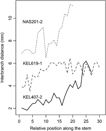
There is a clear increase in measures pertaining to branching morphology along the stem. Moving distally, branches are more widely spaced (Figure 4). The same observation was made for the orthostiche interval and the distance from the stem to the first internode on a branch. This pattern was more or less important, depending on the colony. For KEL407-2, the interbranch distance is about 2 mm toward the base, and between 5 and 6 mm toward the tip. These allometric differences also appeared between the different colonies of haplotype E (Figure 3). Only a juvenile (VER202-1) and an adult (NAS204-1) were successfully sampled for this haplotype (Figure 12, and comments in the Systematics section). All morphological measures (except the angle between branches) were larger for the adult, even the height and width of polyps (Figure 3).
Plot of the distance between branches along the stem, ordered from near the base to near the tip of the colony. NAS201-2 belongs to Chrysogorgia tricaulis sp. nov. (haplotype A). KEL619-1 and KEL407-2 belong to Chrysogorgia artospira sp. nov. (haplotype B).

Sclerite size-distribution
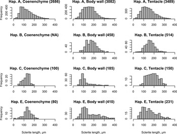
A total of 11,385 sclerites from polyps of all available colonies were measured. The range of sclerite lengths did not vary significantly among the four haplotypes, and among the three polyp body compartments considered (branch coenenchyme, body wall and tentacles). There were some more substantial differences among haplotypes in the mean and skew of the sclerite lengths distributions (Figure 5). Not all haplotypes possessed sclerites in the coenenchyme (see taxonomic description). The distributions were highly right-skewed for sclerites from the polyp body wall in haplotypes C and E. These two haplotypes are characterized by a mix of sclerite types in different proportions: scales are small but abundant, and rods are much larger but scarcer. Despite these differences, there is no indication that sclerite length per se can be used as a diagnostic character.
Distribution of sclerite length (µm) from the coenenchyme, polyp body wall and tentacles of the four msh1 haplotypes (Hap). Sample size is given in parentheses for each group.

There were significant differences between the sclerite length-distributions from different individuals of haplotype A. Some polyps, for example, had smaller sclerites, regardless of the polyp body compartment. Examples are GOO110-2 and MIL101-5. Differences are particularly strong in the coenenchyme. BAL211-1, for instance, is characterized by a bimodal distribution, with a group averaging 80 µm length, and another averaging 190 µm length. While no sclerite >50 µm was measured in the coenenchyme of GOO110-2, LYM310-1 had sclerites as long as 330 µm in this compartment.
Chrysogorgia Duchassaing & Michelotti, 1864: 13 (107). Verrill, 1883: 21; Studer, 1887: 41; Wright & Studer, Reference Wright and Studer1889: xli, 23; Versluys, Reference Versluys1902: 17–33; Nutting, 1908: 588; Kükenthal, 1919: 505–511, 1924: 388–390; Deichmann, 1936: 227–228; Hickson, 1940: 307; Madsen, Reference Madsen1944: 49; Bayer, 1956: F216; Bayer & Stefani, 1988: 259; Williams, 1992: 252; Cairns, Reference Cairns2001: 754, Reference Cairns2007: 512.
Dasygorgia Verrill, 1883: 21; Studer, 1887: 41; Wright & Studer, Reference Wright and Studer1889: xli, 6–9, 278.
TYPE SPECIES
Chrysogorgia desbonni Duchassaing & Michelotti, 1864, by monotypy.
DIAGNOSIS
Colony branching is sympodial, in the form of an ascending spiral (clockwise or counterclockwise), a fan (planar colony), or two fans emerging from a short main stem (biflabellate colony). Axis with a metallic shine, dark to golden in colour. Branches divide dichotomously or pinnately. Most polyps large relative to the size of the branches they sit on. Sclerites in the form of spindles, rods and scales with little ornamentation.
DISCUSSION
Wright & Studer (Reference Wright and Studer1889) proposed to place Chrysogorgia species into two categories based on the zonation of sclerite types (scales and rods/spindles) in the polyp. The ‘Spiculosae’ (also called Group A) consists of species that have rods and or spindles in the polyp body wall and tentacles. The ‘Squamosae typicae’ (Group C) consists of species with scales in the polyp body wall and tentacles. Versluys (Reference Versluys1902) defined the ‘Squamosae aberrantes’, a group intermediate between Groups A and C. This Group B is defined by species with scales in the polyp body wall and rods/spindles in the tentacles. Groups were further divided based on branching sequence.
REMARKS
Cairns (Reference Cairns2001) provided a detailed diagnosis of the genus, and listed the 59 valid species of Chrysogorgia and reviewed the North Atlantic species. He later described one additional species from Antarctica (Cairns, Reference Cairns2002) and two new species from north-eastern Pacific seamounts (Cairns, Reference Cairns2007), with Chrysogorgia pinnata being the first described pinnately-branching species. Pante & France (Reference Pante and France2010) recently described Pseudochrysogorgia, a new chrysogorgiid genus that closely resembles Chrysogorgia morphologically, but is most closely related to Metallogorgia based on a multi-gene phylogeny.
DISTRIBUTION
Known from all ocean basins between 100 and 3375 m depth (Cairns, Reference Cairns2001); the depth limit of Chrysogorgia colonies from this study is 3860 m and extends Cairns' range by almost 500 m. Recently, ROV-based exploration revealed the presence of Chrysogorgia between 4163 and 4492 m depth on Derickson Seamount in the Gulf of Alaska (specimen deposited at the Smithsonian Institution, catalogue number USNM 1081181).
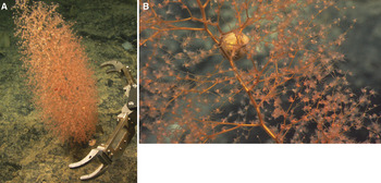
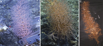
Chrysogorgia tricaulis sp. nov. (haplotype A). In situ photographs of holotype KEL613-1 (A) and paratype GOO108-1 (B) before and during collection, respectively.

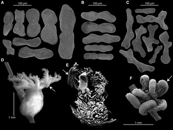
Chrysogorgia tricaulis sp. nov. (haplotype A; A-D: KEL613-1, holotype; E: NAS201-2, paratype; F: GOO108-1, paratype). (A) Sclerites from the polyp body wall; (B) sclerites from the branch coenenchyme; (C) sclerites from tentacles; (D) light microscopy of an entire polyp; (E) scanning electron microscopy (SEM) of a partially digested polyp; (F) SEM of the tentacles and their uncharacterized features (arrows).

TYPE MATERIAL
Holotype: Kelvin Seamount, New England Seamount Chain, Station 613, 38°45.93N 64°05.43W, 2132 m depth, 31 August 2005, YPM 38607, Isolate KEL613-1, GenBank ID GQ180126.
Paratypes: Goode Peak, CS, Station 108, 35°23.58′N 51°16.02'W, 2068 m depth, 21 August 2005, YPM 38590, Isolate GOO108-1, GenBank ID GQ180128; Kelvin Seamount, NES, Station 202, 38°51.59′N 63°54.85'W, 2158 m depth, 16 July 2003, YPM 38609, Isolate KEL202-2; Kükenthal Peak, Corner Seamount, CS, Station 203, 35°33.40′N 51°48.87′W, 1859 m depth, 22 August 2005, YPM 38589, Isolate KUK203-1, GenBank ID GQ180129; Nashville Seamount, NES, Station 201, 34°28.19′N 56°43.77′W, 2529 m depth, 25 August 2005, YPM 38598, Isolate NAS201-2.
COMPARATIVE MATERIAL EXAMINED
Balanus Seamount, NES, Station 211, 39°24.76′N 65°24.48′W, 1689 m depth, 1 September 2005, YPM 38602, Isolate BAL211-1, GenBank ID GQ180125; Bear Seamount, NES, Station 401, 39°57.1′N 67°24.78′W, 1559 m depth, 11 May 2004, YPM 38608, Isolate BEA401-1, GenBank ID GQ180123; Goode Peak, CS, Station 110, 35°23.58′N 51°16.12′W, 2000 m depth, 21 August 2005, YPM 38601, Isolate GOO110-2; Kelvin Seamount, NES, Station 601, 38°45.45′N 64°05.46′W, 2593 m depth, 31 August 2005, YPM 38603, Isolate KEL601-4; Yakutat Seamount, CS, Station 201, 35°11.5N 47°40.3W, 2379 m depth, 14 August 2005, YPM 38593, Isolate LYM201-2, GenBank ID GQ180131; Yakutat Seamount, CS, Station 310, 35°22.16′N 48°09.54′W, 1533 m depth, 15 August 2005, YPM 38595, Isolate LYM310-1; Milne Edwards Peak, Caloosahatchee Seamount, CS, Station 101, 34°49.08′N 50°30.37′W, 1689 m depth, 17 August 2005, YPM 38591, Isolate MIL101-5, GenBank ID GQ180130; Nashville Seamount, NES, Station 103, 34°34.98′N 56°50.59′W, 2250 m depth, 24 August 2005, YPM 38592, Isolate NAS103-2 GenBank ID GQ180127; Nashville Seamount, NES, Station 201, 34°28.19′N 56°43.77′W, 2529 m depth, 25 August 2005, YPM 38597, Isolate NAS201-5; Retriever Seamount, NES, Station 101, only small fragments; 39°45.06′N 66°14.94′W, 3860 m depth, 22 May 2004, Isolate RET101-1, GenBank ID EU268056.
DIAGNOSIS
Wide bottlebrush colony with a 1/3L (counterclockwise) spiral and a large orthostiche interval. Branches stiff and straight. Pitcher-shaped polyps on the main stem and branches, placed on internodes and nodes. Sclerites in the form of scales in the branch coenenchyme (abundant), polyp body wall and tentacles, diagnostic of the Squamosae typicae. msh1 haplotype A.
DESCRIPTION
The holotype is 42 cm tall and 19 cm wide. It was collected from a hard substrate, and cut by the ROV manipulator arm very close to its base. In situ photographs show a white/yellow discoidal holdfast for this specimen. Some colonies (NAS201-2 and GOO108-1) were collected with their discoidal holdfast. The colony consists of a wide 1/3L spiral, and when viewed from below shows three large passageways produced by the regularity of the branching. The stem has a deep golden colour and a metallic lustre. It is stiff and significantly thicker than the base of branches along most of the colony (proximal area: stem at least twice as thick as branches; distal area: stem and branches almost equally thick). Every time it gives off a branch, the stem deviates from the main axis, producing a zigzag pattern typical of Chrysogorgia. On the holotype, the interbranch distance varies between 6 and 15 mm (average 11 mm ± 2; all specimens: 10 ± 3 mm, 4–30 mm, N = 219), and the orthostiche interval is about three times as much (holotype: 30.7 ± 5.6 mm, 16.7–38.9 mm, N = 23; all specimens: 27 ± 7 mm, 14–42 mm, N = 124). Branches are as stiff as the stem at their base (diameter, holotype: 1.1 ± 0.2 mm, 0.8–1.4 mm, N = 12; all specimens: 0.7 ± 0.3 mm, 0.1–1.6 mm, N = 148), and thinner and more flexible toward their tip. They emerge from the main stem at an obtuse angle (holotype: 121.8 ± 11.6°, 106.3–135.9°, N = 12; all specimens: 114 ± 11°, 93–144°, N = 95) at regular intervals. Branches are straight, some (the most distal) having a slight curvature. Branching occurs in multiple planes, and branching order varies along the colony, the middle being the bushier part of the colony (10th order of branching). Among the rest of the specimens, branching order varies between 3 (small colony KEL601-4) and 19 (NAS201-2). Anastomosing of branches was never observed. The angle between subdividing branches is regularly acute (holotype: 76.2 ± 10.2°, 59.3–95.5°, N = 15; all specimens: 77 ± 14°, 47–121°, N = 250). The distance between the stem and first branch node (holotype: 12.1 ± 2.9 mm, 8.6–18.3 mm, N = 11; all specimens: 13 ± 3 mm, 5–21 mm, N = 117) is similar to the interbranch and the internode distances, although the internode distance may slightly decrease toward the tip of the branch. The size of the terminal branchlet directly correlates with the number of polyps that sit on it.
Polyps are orange while alive and turn white in ethanol. All colonies are characterized by axial polyps placed on the interbranch. In most cases, one polyp is placed on branch nodes, and one is placed on branch internodes. The number of polyps per internode most commonly is one, but two or three polyps can be observed, in which case they are equally spaced. Branch tips carry one to four polyps, but most have one or two. On average, polyps are oriented upwards. Most are in the shape of pitchers, and are almost as wide (holotype: 0.8 ± 0.2 mm, 0.5–1.2 mm, N = 15; all specimens: 1 ± 0.3 mm, 0.4–2.4 mm, N = 309) as they are tall (holotype: 1.2 ± 0.2 mm, 1–1.6 mm, N = 17; all specimens: 1.1 ± 0.3 mm, 0.5–2.3 mm, N = 320). Cnidal papillae are present on the polyp body. On some polyps, the back of the tentacles is almost entirely covered by sclerite-free tissue resembling a gland (Figure 7D–F). To date, these features are of unknown origin and function, although they do not appear to be larvae or parasites (Watling & Simpson, unpublished histological examination).
Sclerites of the polyp body are in the form of smooth scales. In the coenenchyme, they are elongated, with a slight constriction in the middle, and run parallel to the branch (all specimens: 126 ± 57 µm, 17–334 µm, N = 2686). Sclerites in the polyp body wall can be rounded on their distal ends with a strong constriction in the middle (e.g. Figure 7, 3rd sclerite of the polyp body wall; all specimens: 154 ± 56 µm, 26–441 µm, N = 3082). They are densely packed and arranged parallel to the branch (as in Madsen's (1944) description of C. campanula). The sclerites are found stacked horizontally in the back of the tentacle (perpendicular to the axis of the tentacle), and tend to be smaller and more longitudinally arranged toward the tip of the tentacle (all specimens: 143 ± 60 µm, 19–352 µm, N = 3489). Sclerites rarely extend into the pinnules, which are otherwise sclerite-free. Tentacle sclerites are smooth, flat scales or idiosyncratic shapes.
ETYMOLOGY
Species epithet is Latin for ‘three passages’ (tri and caulus in combination) in reference to the large passageways visible when the colony is viewed from below.
DISTRIBUTION
This species was found throughout the NES and CS chains, from Bear Seamount (north-western) to Yakutat Seamount (south-eastern), from 1533 m to 3860 m depth. With fifteen colonies, this is the most abundant species collected on the NES and CS.
REMARKS
Paratypes were chosen to cover the range of variation revealed by the PCA. Colony silhouette varies across specimens. While most are tall bottlebrushes, much taller than they are wide, some are as wide as they are tall. For example, NAS201-2 is 27 cm tall and 30 cm wide, while KEL613-1 (holotype) is 42 cm tall and 19 cm wide. Ten of the 14 colonies examined have a very regular 1/3L branching pattern. However, variation was observed in four specimens (GOO108-1, LYM201-2, KEL202-2 and NAS103-2). One of them is particularly noteworthy: 10 cm from the holdfast, the axis of the GOO108-1 shifts by 43°, perhaps indicative of a response to the overall position of the colony relative to environmental conditions such as current flow. Also, most of the branches of LYM201-2 fell off shortly after fixation. The size–frequency of sclerites was variable between polyps from different colonies (see Results section). Multiple colonies were found with egg cases of an unknown ‘dumbo’ octopus (KEL613-1, GOO110-2, BAL211-1 and LYM310-1) and the shrimp Bathypalaemonella serratipalma Pequegnat, 1970 (KEL613-1 and BAL211-1). While fourteen colonies were examined, we obtained a few branch fragments from a fifteenth one (RET101-1), which corresponds to the deepest occurrence of msh1 haplotype A, and is the deepest recorded occurrence of any species in the genus.
COMPARISONS
There are eight species of Squamosae typicae (Group C) with a 1/3L branching sequence, none of which fit the description of Chrysogorgia tricaulis sp. nov. Chrysogorgia axillaris (Wright & Studer, Reference Wright and Studer1889) and C. geniculata (Wright & Studer, Reference Wright and Studer1889) are short, flexible colonies with interbranch and orthostiche distances that are significantly shorter than documented here. According to Versluys (Reference Versluys1902), C. rigida Versluys, Reference Versluys1902 is almost identical to C. geniculata, and these could belong to the same species. Chrysogorgia cavea Kinoshita, Reference Kinoshita1913 is a very robust, short bush. Its mode of colony growth is strikingly different from that of C. tricaulis sp. nov. (photograph in Kinoshita, Reference Kinoshita1913). Chrysogorgia sibogae Versluys, Reference Versluys1902 (described from one specimen) is a short colony with very tightly-spaced branches (1–3 mm), few branch internodes and a significant disparity between the lengths of the proximal and distal branch internodes. Chrysogorgia excavata Kükenthal, 1908 has very particular tentacular sclerites, in the form of elongated, curved needles with a serrated edge (Kükenthal, 1908: figures 45 & 47). The branches of that species are not fully bifurcating, producing a lyrate appearance in places (Kükenthal, 1908: figure 44). The description of C. delicata Nutting, 1908 is very succinct, and based on 5 cm of a single, damaged colony. It differs from C. tricaulis sp. nov. by a short interbranch distance (4 mm), longitudinally arranged sclerites in the polyp body wall, and curved, transversally-arranged tentacular sclerites. Chrysogorgia fruticosa (Studer, 1894) is a short colony with a short interbranch distance, and the mode of branch ramification (‘Cyma helicoidea unipara’) is different from that observed in C. tricaulis sp. nov.
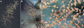
Chrysogorgia artospira sp. nov. (haplotype B). In situ photographs of (A) holotype KEL407-2 and (B) paratype MIL102-3 during collection; (C) paratype KEL619-1 photographed in the laboratory aboard ship.

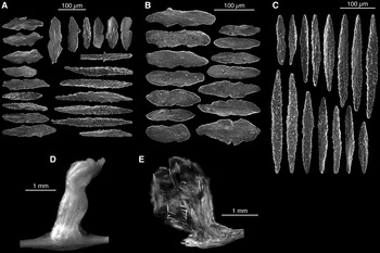
Chrysogorgia artospira sp. nov. (haplotype B; KEL407-2, holotype). (A) Sclerites from the polyp body wall; (B) sclerites from tentacles; (C) light microscopy (LM) of a polyp; (D) scanning electron microscopy of a polyp; (E) ) LM of a polyp cleared with clove oil to reveal the arrangement of sclerites (photograph inverted).

TYPE MATERIAL
Holotype: Kelvin Seamount, NES, Station 407, 38°46.98′N 63°57.77′W, 2253 m depth, 19 May 2004, YPM 38596, Isolate KEL407-2, GenBank ID GQ180132.
Paratypes: Kelvin Seamount, NES, Station 619, 38°46.23′N 64°05.56′W, 1965 m depth, 31 August 2005, YPM 38605, Isolate KEL619-1, GenBank ID GQ868346; Kükenthal Peak, Corner Seamount, CS, Station 205, 35°33.41′N 51°48.89′W, 1846 m depth, 22 August 2005, YPM 38604, Isolate KUK205-1, GenBank ID GQ180133; Milne Edwards Peak, Caloosahatchee Seamount, NES, Station 102, 34°48.99′N 50°30.36′W, 1650 m depth, 17 August 2005, YPM 38599, Isolate MIL102-3, GenBank ID GQ180134.
DIAGNOSIS
Elongated bottlebrush colony with a 2/5L (counterclockwise) spiral and a short orthostiche interval. Branches straight and stiff. Pitcher-shaped polyps on the main stem and branches, placed on internodes and nodes. Sclerites in the form of scales in the polyp body wall and tentacles, diagnostic of the Squamosae typicae. Sclerites rare or absent from the branch coenenchyme. msh1 haplotype B.
DESCRIPTION
The holotype is a narrow bottlebrush colony, 25 cm tall and 11 cm wide. It was collected with its discoidal holdfast. The colony consists of a narrow 2/5L spiral. The stem has a brown-golden colour and the metallic lustre typical of Chrysogorgia. Every time it gives off a branch, the stem deviates from the main axis, producing a zigzag pattern. The stems of older colonies have a darker colour. About 4 cm from the holdfast, a side branch forms a secondary stem, itself characterized by a regular, narrow 2/5L spiral. It is stiff and significantly thicker than the basal branches along most of the colony (proximal area: stem over twice as thick as branches; distal area: stem and branches almost equally thick). The interbranch distance is short (holotype: 3.3 ± 1.3 mm, 1.8–6.2 mm, N = 27; all specimens: 4 ± 1 mm, 2–10 mm, N = 122). Moving distad along the stem, the interbranch distance progressively increases from about 2 mm to almost 6 mm (Figure 5). The orthostiche distance is about five times the interbranch distance (holotype: 18.8 ± 2.4 mm, 15–21 mm, N = 8, all specimens: 20 ± 4 mm, 11–30 mm, N = 74). Branches are as stiff as the stem at their base (diameter, holotype: 0.7 ± 0.2 mm, 0.4–1.2 mm, N = 24; all specimens: 0.7 ± 0.3 mm, 0–1.3 mm, N = 55), and thinner and more flexible toward their tip. They emerge from the main stem at an obtuse angle (holotype: 121 ± 10.8°, 102.7–134.8°, N = 10; all specimens: 121 ± 9°, 97–138°, N = 45) at regular intervals. On average, the internodes are as short as the interbranch distance (distance between the stem and the first internode, holotype: 4.7 ± 1.6 mm, 2.4–6.5 mm, N = 10; all specimens: 6 ± 1 mm, 2–9 mm, N = 56). Branching occurs in multiple planes, and branching order is stable along the colony, varying between the 6th and the 8th order. There is no evidence of anastomosing between the branches of the holotype, but two of the four colonies examined exhibited fused branches (KUK205-1 and MIL102-3). The angle between subdividing branches is regularly acute (holotype: 76.3 ± 10.5°, 60.3–89.4°, N = 7; all specimens: 87 ± 12°, 60–117°, N = 59), and the internode length tends to decrease from the first node on.
Polyps are orange while alive and turn white in ethanol. Axial polyps were observed on none of the colonies examined. There is one polyp per branch node (or just next to the node) on the holotype, and other examined colonies can carry between zero to two polyps on the internode in addition to the polyp situated directly on or next to the node. Branch tips carry one or two polyps. This is the general case, but up to five polyps can be observed on the terminal branchlet. Polyps overall are oriented upward, with many exceptions. They are on average as wide (holotype: 1.1 ± 0.3 mm, 0.6–1.4 mm, N = 20; all specimens: 0.9 ± 0.3 mm, 0.6–1.7 mm, N = 76) as they are tall (holotype: 1.3 ± 0.3 mm, 0.8–1.9 mm, N = 40; all specimens: 1.1 ± 0.3 mm, 0.4–1.9 mm, N = 100), and can be slightly constricted at the neck. No cnidal papillae were observed on the polyp or the branch coenenchyme.
Throughout the polyp body, sclerites are in the form of smooth scales (all specimens: 174 ± 48 µm, 62–338 µm, N = 458). They are absent from the branch coenenchyme. In the polyp body wall, sclerites are densely packed and arranged parallel to the branch in a way that is very similar to what is observed in Chrysogorgia tricaulis sp. nov. They are rounded on their distal ends with a constriction in the middle. Some short rods (some curved) can occasionally be observed (seen in KEL407-2 and KUK205-1). Sclerites are found stacked laterally in the back of the tentacle (perpendicular to the axis of the tentacle; all specimens: 161 ± 42 µm, 40–309 µm, N = 514). These are smooth, flat scales or idiosyncratic shapes. Some rare sclerites partially extend into the pinnules, which are otherwise sclerite-free. These sclerites do not appear any different from the other sclerites found in the tentacles.
ETYMOLOGY
Species epithet is Latin for ‘tight spiral’ (arto and spira combined) in reference to the 2/5 branching sequence, the tightest spiral for any colony of Chrysogorgia observed on the NES and CS.
DISTRIBUTION
Species known from Kelvin Seamount, located approximately in the middle of the NES, as well as Corner and Caloosahatchee Seamounts on the CS. Depth-distribution extends from 1650 to 2253 m.
REMARKS
This species was found in association with egg cases of an unknown ‘dumbo’ octopus (KEL619-1 and MIL102-3), fish eggs (MIL102-3), a comatulid crinoid (MIL102-3), scale worms (KEL407-2, KEL619-1) and a cladorhizid carnivorous sponge (KEL619-1).
COMPARISONS
Based on the list of valid species compiled by Cairns (Reference Cairns2001), only three species of the Squamosae typicae are characterized by a 2/5L spiral: C. acanthella (Wright & Studer, Reference Wright and Studer1889), C. pendula Versluys, Reference Versluys1902 and C. campanula Madsen, Reference Madsen1944. While the first two were described from the south-western Pacific (Kermadec, 1097 m, and Banda Sea, 1595 m), C. campanula was described from Icelandic waters (2448 m), and might therefore be closely related to Chrysogorgia artospira sp. nov. Madsen (Reference Madsen1944) noted that this species seems ‘more closely related to C. acanthella (Wright & Studer), from which it may, however, be distinguished by its larger zooids, the absence of cnidal papillae, and its much closer layer of scales in the coenenchyma.’ The polyps of C. campanula are indeed stout and densely packed with sclerites. They have a ‘trumpet’ shape (the width of the polyp increases from its base upwards) that Chrysogorgia artospira sp. nov. clearly lacks. The tentacles of C. campanula are thicker than those of Chrysogorgia artospira sp. nov. Although the interbranch distances (3–3.5 mm) and internodal distances (2.5–9 mm) reported by Madsen (Reference Madsen1944) are similar to ours, the colony examined by Madsen was 8.5 cm tall, while the specimens we examined were no smaller than 23 cm in height (this height difference may simply reflect an age difference). Both C. campanula and C. acanthella differ from Chrysogorgia artospira sp. nov. by the presence of polyps on the stem and sclerites in the branch coenenchyme. Chrysogorgia acanthella has abundant verrucae in the coenenchyme (giving it a rugged appearance) and an interbranch distance of 1.5 mm. Chrysogorgia pendula was described from part of a highly damaged colony characterized by unusual descending size branches. This species has an abundance of sclerites in the branch coenenchyme.
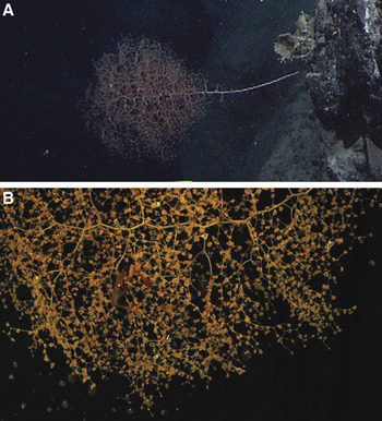
Chrysogorgia averta sp. nov. (haplotype C; LYM201-1, holotype). (A) In situ and laboratory photographs.

Chrysogorgia averta sp. nov. (haplotype C; LYM201-1, holotype). (A) Sclerites from the polyp body wall; (B) sclerites from the branch coenenchyme; (C) sclerites from tentacles; (D) scanning electron microscopy of a mature polyp; (E) light microscopy (LM) of a mature polyp, arrow points to cnidal papillae; (F) LM of a mature polyp treated with clove oil to reveal position of sclerites, arrow points to an egg; (F) LM of an immature polyp treated with clove oil.

TYPE MATERIAL
Holotype: Lyman Peak on Yakutat Seamount, Station 201, 35°11.5N 47°40.3W, 2379 m depth, 14 August 2005, YPM 38594, Isolate LYM201-1, GenBank ID GQ180136.
DIAGNOSIS
Wide bottlebrush colony with a 3/8L (counterclockwise) spiral and a very wide orthostiche interval. Branches slightly curved, forming ‘U’-shaped bifurcations. Polyps long and narrow, placed on the internodes, not on the nodes. Sclerites in the form of flat rods and scales in the branch coenenchyme, rods and scales in polyp body wall, and rods in tentacles (diagnostic of the Spiculosae). msh1 haplotype C.
DESCRIPTION
This species is described from a single specimen. The holotype is 42 cm tall and 25 cm wide. It was collected from a tall colony, the main stem having been cut by the ROV manipulator claw near the base of the colony. Based on extrapolation from laboratory and in situ photographs, the colony was about 45 cm tall. The holdfast is a very small disc, about 1–2 cm diameter. The colony consists of a wide 3/8L spiral. The stem has a golden colour with a faint green tinge and a metallic lustre. Every time it gives off a branch, the stem deviates from the main axis, producing a zigzag pattern. The stem is stiff and significantly thicker than the base of branches along most of the colony (proximal area: stem twice as thick as branches; distal area: stem and branches almost equally thick). The interbranch distance varies between 9 and 13 mm (average 11 ± 1 mm), and the orthostiche interval is particularly long (76 ± 1 mm, 75–78 mm, N = 4). Branches are as stiff as the stem at their base (diameter: 1.1 ± 0.2 mm, 0.8–1.6 mm, N = 14), and thinner and more flexible toward their tip. They emerge from the main stem at an obtuse angle (104 ± 10°, 97–122°, N = 10) at regular intervals. Internodes are characterized by a slight curvature; bifurcations are ‘U’-shaped as a result (this curvature makes the angle between bifurcating branches particularly obtuse: 108 ± 10°, 91–124°, N = 15). Branching occurs in multiple planes, and branching order varies along the colony (base: 6th–8th order, middle: 9th–12th order, top: 10th order). There is no evidence of anastomoses between branches. The distance between the stem and the first branch node is 17 ± 2 mm (13–19 mm, N = 6), and the internodal distance progressively decreases moving distad (size of branchlet: 8 ± 4 mm).
Polyps are yellow/orange while alive and turn white in ethanol. Axial polyps were not observed, and polyp occurrence most often starts on the first branch internode. Most internodes carry zero to two polyps, most commonly one to two. Polyps are equally spaced on the internodes, and are not found on the nodes. Terminal branchlets carry one to three polyps, but most have one. Most polyps are oriented up and outwards. They are on average longer (1.5 ± 0.3 mm, 1.1–1.9 mm, N = 13) than they are wide (0.7 ± 0.1 mm, 0.5–1 mm, N = 20), and are slightly constricted at the neck. Cnidal papillae are present on the polyp body wall and the branch coenenchyme (Figure 11E). Egg-bearing polyps are characterized by two pouches that sit on each side of the branch, as if they were saddle bags (Figure 11D; arrow pointing to an egg: Figure 11F).
The branch coenenchyme contains few, small sclerites in the form of rods (122 ± 30 µm, 43–182 µm, N = 100). The polyp body wall contains scales (most abundant; 96 ± 23 µm, 41–196 µm, N = 150) and rods (more or less blunt-ended; 181 ± 60 µm, 79–334 µm, N = 35). Sclerites are longitudinally arranged in the polyp body. Scales and rods are particularly abundant at the base. Moving distad along the polyp body wall, rods become larger and more aggregated in the grooves between the tentacles. At the oral disc, rows of sclerites from adjacent grooves meet at the tentacle base and form longitudinal rows, four to five sclerites wide, along the back of the tentacle (186 ± 53 µm, 62–301 µm, N = 150). Tentacles contain rods only, and pinnules are free of sclerites.
ETYMOLOGY
Species epithet is Latin for ‘saddle bag’, in reference to the morphology of mature polyps, with their two ‘pockets’, containing eggs and extending below each side of the branch.
DISTRIBUTION
Only known from the north-western Atlantic at the type location, namely Lyman Peak, Yakutat Seamount in the CS chain, 2379 m depth.
REMARKS
The zonation of sclerite types (rods present in the tentacles and polyp body wall) places this species in the Spiculosae (Group A). The holotype was collected with the shrimp Bathypalaemonella serratipalma Pequegnat, 1970.
COMPARISONS
This species represents the first recorded occurrence of the 3/8L branching sequence. Chrysogorgia herdendorfi Cairns, Reference Cairns2001, described from deep waters off the coast of South Carolina, is characterized by a 2-5R–3/8R spiral. This latter species is characterized by significantly shorter interbranch (2.5–3 mm), orthostiche (14–17 mm) and stem-to-first branch node (4–7 mm) distances. Also, the branches of C. herdendorfi emerge from the main stem with a more obtuse angle (i.e. they are more pointed toward the top of the colony), and the colony is significantly more slender than Chrysogorgia averta. Finally, branches are not nearly as stout, and do not arc as do the branches of C. averta. These differences, however, could be attributed to growth, as the maximum height for C. herdendorfi is 22 cm, half the size of C. averta. Other parameters (sclerite composition and number of polyps on first internode) are congruent, and these species may be closely related. Both species were collected from the north-western Atlantic from similar depths, and while C. averta was collected on a seamount (on the upper edge of a wall) C. herdendorfi was collected from a wreck.
Chrysogorgia abludo sp. nov. (haplotype E). Photographs of (A) holotype VER202-1 (laboratory) and (B) paratype NAS204-1 (in situ); (C) close-up of the polyps and associate of NAS204-1.

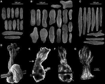
Chrysogorgia abludo sp. nov. (haplotype E; VER202-1, holotype). (A) Sclerites from the polyp body wall; (B) sclerites from the branch coenenchyme; (C) sclerites from tentacles; (D) light microscopy (LM) of polyp; (E) LM of polyp treated with clove oil to reveal position of sclerites.

TYPE MATERIAL
Holotype: Verrill Peak, Caloosahatchee Seamount, CS, Station 202, 34°31.84′N 49°47.39′W, 2110 m depth, 19 August 2005, YPM 38606, Isolate VER202-1, GenBank ID GQ180139. Paratype: Nashville Seamount, NES, Station 204, 34°28.73′N 56°44.04′W, 2121 m depth, 25 August 2005, YPM 38600, Isolate NAS204-1.
COMPARATIVE MATERIAL EXAMINED
Nashville Seamount, NES, Station 102, fragments only; 34°34.97′N 56°50.60′W, 2246 m depth, 24 August 2005, Isolate NAS102-3, GenBank ID GQ180138.
DIAGNOSIS
Wide bottlebrush colony with a 1/3L, 1/4L or irregular (counterclockwise) spiral. Polyps with a strong constriction at the neck, placed on internodes and nodes. Polyps absent from the main stem. Sclerites in the form of scales in the coenenchyme, scales and rods in the polyp body wall, and rods in the tentacles (diagnostic of the Spiculosae). msh1 haplotype E.
DESCRIPTION
The holotype is a small, narrow, sparsely branched colony with a bottlebrush shape. It is 16 cm tall and 7 cm wide. The paratype NAS204-1 is much taller (29 cm) and wider (24 cm), but in very poor condition, most branches having fallen off the stem after fixation of the specimen. It is not bottlebrush-shaped, but rather a bush of branches perched on top of a long stem. From in situ photographs, it can be estimated that the colony was about 50 cm tall, 20 cm wide, and started branching about 20 cm from its base. The holdfast of the holotype is only slightly visible in the in situ photographs, and appears to be a small disc attached to some exposed basalt with a veneer of biogenic sand. In the paratype the holdfast is a small disc about 1 cm diameter. Colonies are golden with a metallic lustre and have a counter-clockwise (L) spiral. The branching sequence is irregular, 1/3 or 1/4 in places. The holotype is slender, but the paratype is stiff, with thick axis (diameter 2.2 mm at the base) and branches (diameter at the base: 0.9–1 mm, N = 2). In both specimens, the axis is thicker than the branches near the base, but gets thinner when moving distad. Towards the tip of the colonies, the stem is as thick as the side branches. Every time it gives off a branch, the stem deviates from the main axis, producing a zigzag pattern typical of Chrysogorgia. The interbranch distance is short on the holotype (5.1 ± 0.6 mm, 4.3–6.8, N = 20) and twice as long on the paratype (10.7 ± 3 mm, 7.5–15, N = 9). Branches emerge from the main stem at an obtuse angle (holotype: 98.4 ± 5.9°, 92.3–109.3°, N = 9; paratype: 112.4 ± 2.7°, 110.5–114.3°, N = 2) at regular intervals. The distance from the stem to the first interbranch is 8.5 ± 2.1 mm (6.1–11 mm, N = 6) on the holotype. This parameter could only be measured in two instances on the paratype, and is about 16 mm in both cases. The angle between subdividing branches is acute (holotype: 92.2 ± 8.5°, 83.3–102.2°, N = 4; paratype: 72.3 ± 11.6°, 54.7–86.3°, N = 10). They bifurcate only once or twice on the holotype. Branching order is much higher in the paratype, although this parameter is hard to assess due to the poor preservation of the specimen. While anastomoses were not observed on the holotype, fused polyps (different polyps attached at their base) were observed on the paratype. On the holotype, internodes bear one or two polyps, one being close to the node. This character cannot be assessed from the paratype. Terminal branchlets bear one to three polyps on the holotype, and one to six polyps on the paratype.
Polyps are orange while alive and turn white in ethanol. Axial polyps were not observed. Polyps are mostly oriented upward. They are on average longer (both specimens: 1.5 ± 0.4 mm, 0.8–2.2 mm, N = 27) than they are wide (both specimens: 0.9 ± 0.2 mm, 0.6–1.4 mm, N = 27), and are strongly constricted at the neck. No cnidal papillae were observed on the polyp or the branch coenenchyme.
The branch coenenchyme bears small, rugged scales (both specimens: 135 ± 40 µm, 19–238 µm, N = 80). In the polyp body wall, sclerites are in the form of rods (both specimens: 227 ± 78 µm, 60–399 µm, N = 160) and smooth, elongated scales of idiosyncratic shapes (both specimens: 120 ± 43 µm, 38–251 µm, N = 250). They are mostly found transversally and longitudinally arranged (i.e. parallel to the polyp axis). The tentacles contain rods exclusively (both specimens: 154 ± 67 µm, 42–356 µm, N = 231), and pinnules are free of sclerites. Rods form longitudinal rows, four to five sclerites wide along the back of the tentacle.
ETYMOLOGY
Species epithet is Latin for ‘dissimilar’, in reference to the different overall morphologies of the colonies examined, including the branching sequence.
DISTRIBUTION
Known from the CS (Caloosahatchee Seamount) and the southern tip of the NES (Nashville Seamount), between 2110 and 2246 m depth.
REMARKS
While VER202-1 is the smallest colony of this species (and the smallest Chrysogorgia collected on the NES and CS), and therefore probably a juvenile colony, it was chosen over NAS204-1 as the holotype for its better preservation. A third colony (NAS102-3) corresponding to haplotype E was collected. However, everything but a few branches was lost during an ROV manoeuvre. Based on in situ photographs, this colony was bottlebrush-shaped, and much taller (about 60 cm) than it was wide (about 13 cm). It had a discoidal holdfast, and was bifurcating about 21 cm from its holdfast, in a manner very similar to what was described for KEL407-2. This colony started branching 15 cm from the holdfast. Both specimens collected were host to the shrimp Bathypalaemonella serratipalma Pequegnat, 1970.
COMPARISONS
Only one species of Spiculosae (group A) was described with an irregular counter-clockwise spiral (Cairns, Reference Cairns2001): C. dichotoma Thomson & Henderson, Reference Thomson and Henderson1906. This specimen, described from the Bay of Bengal at 165 m depth, is among the shallowest Chrysogorgia reported to date. Chrysogorgia abludo sp. nov. differs from this species in its mode of branching (internode distance 10+ mm, and see Plate 6, figure 3 of Thomson & Henderson, Reference Thomson and Henderson1906), polyp arrangement (polyps are aligned, and do not form a spiral) and morphology of polyps (long, narrow with strong constriction; not short and conical). The Spiculosae group does not contain species with a 1/3L spiral. However, it contains 12 1/4L turners (some parts of VER202-1 conform to a 1/4L sequence), all from the Indo-Pacific, mostly from depths much shallower than what was observed for C. abludo (146–1901 m). None of those species conform to the morphology of C. abludo sp. nov.; most are small bushes with a very short interbranch distance (C. cupressa (Wright & Studer, Reference Wright and Studer1889), C. lata Versluys, Reference Versluys1902, C. tetrasticha Versluys, Reference Versluys1902, C. pusilla Versluys, Reference Versluys1902, C. dispersa Kükenthal, 1908, C. minuta Kinoshita, Reference Kinoshita1913 and C. sphaerica Aurivillius, 1931). Others are small bushes with a larger interbranch distance (C. rotunda Kükenthal, 1908, C. okinensis Kinoshita, Reference Kinoshita1913), or have other inconsistent characters (C. pyramidalis Kükenthal, 1908, C. comans Kinoshita, Reference Kinoshita1913: bottlebrush, short interbranch, very long, whip-like branches; C. papillosa Kükenthal, 1908: profusion of papillae).
DISCUSSION
Species delimitation and identification
The four msh1 haplotypes were matched to four, non-overlapping morphotypes (PCA; Figure 2), suggesting that the species described here are true evolutionary units rather than artificial groupings. These results underline the usefulness of msh1 as a barcode for Chrysogorgia on the NES and CS chains. As well, the use of PCA was shown to be particularly useful to assign Chrysogorgia specimens to a particular species. Many of the characters used to separate Chrysogorgia species are continuous, and in many cases, there can be significant overlap between character ranges for different species. For example, interbranch distance was shown to be a useful character to separate haplotypes A and B, as the interbranch distance of A was significantly larger than that of B (Kruskal–Wallis rank sum test: χ2 = 204, df = 1, P < 0.001). However, the two distributions still overlap, as the minimum interbranch distance is 4 mm for Chrysogorgia tricaulis sp. nov., while the maximum distance is 10 mm for Chrysogorgia artospira sp. nov. The PCA might prove particularly valuable to examine such overlap between groups of individuals from different species (i.e. overlap between clouds of points from different species on Figure 3), should intermediate morphotypes or haplotypes be collected.
There was a clear trend towards increasing spacing between branches along the stem in the direction of growth (Figure 5). In the case of KEL407-2, the interbranch distance almost triples from its base to its tip. The effect of growth on colony morphometrics has previously been reported (Kinoshita, Reference Kinoshita1913: description of C. aurea), and has strong implications for species identification. It should be taken into account when diagnosing juvenile or older but fragmentary colonies.
This set of specimens exemplifies the difficulty of identifying colonies to the species-level based on in situ images and videos. There is a rapid increase in the number of studies using remotely operated vehicles to survey deep benthic communities and make faunal inventories (e.g. Lundsten, Reference Lundsten2007; Mortensen et al., Reference Mortensen, Buhl-Mortensen, Gebruk and Krylova2008; Lundsten et al., Reference Lundsten, Barry, Cailliet, Clague, DeVogelaere and Geller2009; McClain et al., Reference McClain, Lundsten, Ream, Barry and DeVogelaere2009; 13 abstracts presented at the 12th Deep-sea Biology Symposium in Reykjavík, Iceland, 2010). While this might be an achievable goal at the genus level (in selected biogeographical regions), is it impracticable at the species level within the Chrysogorgiidae. Chrysogorgia is one of the most speciose of the alcyonacean genera (Cairns, Reference Cairns2002). Groups of species can be distinguished using the zonation of sclerite types within the polyp (Groups A, B & C—Wright & Studer, Reference Wright and Studer1889; Versluys, Reference Versluys1902; Cairns, Reference Cairns2001) and branching sequence. While sclerite zonation is impossible to assess from videos, branching sequence is impractical to assess, because of lack of perspective from videos and the profusion of branches in some species (masking the stem and its branching pattern). Differences between species within a set defined by sclerite zonation and branching sequence are subtle, and include characters such as the number of internodes and placement of polyps on branches, orientation of sclerites on the polyp, presence/absence of specialized sclerites, all of which are impractical or impossible to get from photographs or videos. One tempting solution is to identify specimens based on the known distributional range of a particular species. However, most deep-sea octocorals have very poorly known distributional ranges (except for many pennatulaceans, which have relatively well-established bathymetric ranges—G.C. Williams, personal communication), and our genetics-based studies suggest that many taxa have distributions far wider than previously known. Finally using video for faunal inventories is likely to: (1) severely reduce estimates of diversity, as the rate of species discovery is still very high for this group of organisms; and (2) bias estimates of distributional ranges, as the rate of species misidentification could be high.
The limits of barcoding with msh1
All four msh1 haplotypes were recently found on the Bahama Escarpment during the 2009 Bahamas Deep Coral cruise. While the morphology of specimens (branching sequence and sclerites) from two haplotypes (A and E) conforms well to the morphological profile based on the NES and CS samples, morphology of two other haplotypes (B and C) could not be easily predicted based on msh1. Haplotype B, consistently characterized by a 2/5L and a short interbranch distance on the NES and CS, was represented in the Bahamas by 1/3L–1/4L colonies with a long interbranch interval. These colonies, however, belong to the Squamosae typicae (group C; rods in the polyp body wall and tentacles) as would be expected for haplotype B. Because more extensive genetic sampling suggests that haplotype A is derived from haplotype B we can hypothesize that morphological characters (such as branching sequence), can evolve faster than msh1. As a result, Chrysogorgia specimens with identical msh1 sequences may not necessarily belong to the same species, but rather belong to different, recently-diverged sister species. Indeed, this pattern is not uncommon among octocorals (e.g. McFadden et al., Reference McFadden, Benayahu, Pante, Thoma, Nevarez and France2011). We must caution that only about 700 bp of msh1 were used in this study, and additional sequencing will be required to reliably separate specimens from closely-related species. In addition, morphological analysis of the Bahamas material is preliminary, and a more thorough analysis will be required.
Comparisons with north-western Atlantic Chrysogorgia
There is a sharp contrast between the previously-described north-western Atlantic fauna (reviewed in Cairns, Reference Cairns2001) and the specimens collected on the NES and CS.
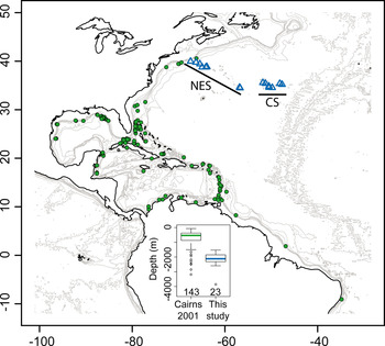
Most species reported by Cairns (Reference Cairns2001) are small (less than 25 cm tall), slender colonies, with closely-spaced branches (interbranch 0.5–6 mm). Three of the nine described species have a rhizoidal holdfast, adapted to soft sediments. Overall, these specimens were sampled from significantly shallower depths, on slope environments (Figure 14). Only 10% of the specimens reported in Cairns (Reference Cairns2001) were collected within the depth-range reported in this study. Those specimens (belonging to C. agassizii, C. elegans, C. fewkesii, C. herdendorfi and C. spiculosa) are all directly associated with the continental slope (from New England to northern Mexico, Columbia and Guyana), and three of the five species represented have a rhizoidal holdfast.
Map of the north-western Atlantic, with the specimens described in Cairns (Reference Cairns2001) and in this study represented by filled circles and open triangles, respectively. The continental slope is made evident by plotting contour lines between 0 and 1000 m depth (200 m intervals). Seamounts are made apparent using contour lines between 1500 and 4000 m depth (1000 m intervals). The depth-distribution of both groups of specimens is presented as an insert (sample size under each boxplot).

In contrast, the specimens presented in this paper were sampled from the summit and flanks of old seamounts of volcanic origin (Sleep, Reference Sleep1990). While the species reported in Cairns (Reference Cairns2001) and the ones described here seem to be sympatrically distributed (Figure 14), they are in fact found in disjunct habitats, as our north-western-most samples were collected on seamounts impinging on the continental margin (e.g. Bear Seamount), and not on the slope itself. In situ photographs confirm that all colonies reported here were sampled directly on hard substrates or lightly sedimented areas, and all four species have encrusting, discoidal holdfasts adapted to attachment to hard surfaces. Previously described north-western Atlantic species may therefore be adapted to different environments, characterized by more sedimented substrates, higher primary productivity and different hydrological regimes.
This hypothesis is supported by our recent observations from the Bahamas Escarpment: all four msh1 haplotypes from the NES and CS were sampled in the Bahamas from deep waters (between 1073 and 2258 m depth) and from hard substrates. The distribution of north-western Atlantic species might, therefore, not be directly affected by the geological origin of the substrate (i.e. continental versus oceanic), but rather its nature (i.e. hard versus soft). Indeed, Metallogorgia melanotrichos (Wright & Studer, Reference Wright and Studer1889), previously thought to be a seamount specialist, was also recently collected from the Bahamas Escarpment.
Finally, sampling strategy might explain why the species described herein were apparently never sampled before. Hard substrates from escarpments and walls were targeted during the NES, CS and Bahamas cruises. These areas, chosen because they are most often associated with accelerated currents preferred by filter-feeding invertebrates such as corals, are difficult or impossible to sample using dredges or trawls.
Atlantic–Pacific connections
All Chrysogorgia colonies collected on the NES and CS have a sinistral (L) spiral. With the exception of C. campanula from the Denmark Strait, off Iceland, all other species from the Atlantic were described with a dextral (R) spiral. Species characterized by a sinistral spiral have been described from the Coral Triangle, Japan, Hawaii and the Gulf of Panama. Two of the four species found on the NES and CS have smooth scales in their polyp body wall and tentacles (Squamosae typicae, Group C). Again, with the exception of C. campanula, this group has previously been described exclusively from Pacific locations. Finally, one species (Chrysogorgia artospira sp. nov.) is represented on the NES and CS by the msh1 haplotype B, which has been sampled twice from Hawaii (e.g. specimen LAD23; Thoma et al., Reference Thoma, Pante, Brugler and France2009). There is no evidence at present that all specimens characterized by haplotype B belong to the same species (see discussion of material from the Bahama Escarpment above). However, these specimens are likely very closely related. These three lines of evidence (direction of the spiral, zonation of sclerite types and msh1 haplotyping) all suggest a faunal connection between the Atlantic and Pacific. This is further supported by the fact that Iridogorgia, Radicipes and Metallogorgia (Chrysogorgiidae) all possess msh1 haplotypes that are shared between Atlantic and Pacific locations (Thoma et al., Reference Thoma, Pante, Brugler and France2009). While the phylogenetic extent and the age of the connection between Atlantic and Pacific will need further investigation, we can hypothesize that this connection was sustained for the major part of the morphological diversification of Chrysogorgia, as all major morphological characters (spiral direction, major branching Groups such as 1/3, 1/4 and 2/5, and sclerite Groups A, B and C) are present in both ocean basins.
ACKNOWLEDGEMENTS
This work was made possible by generous funding provided by the National Oceanic and Atmospheric Administration (NOAA) Ocean Exploration Program (NA66RU0186, NA03OAR4600116, NA05OAR4301001, NA05OAR4601061 and NA08OAR4600756). We would like to thank LW's co-principal investigators, P. Auster, S. France, I. Babb, L. Mullineaux, J. Moore and K. Scanlon for their help in securing the necessary funding to allow us to explore north-western Atlantic seamount communities. The comparative Chrysogorgia material from the Bahamas was recently collected during the NOAA-funded Bahamas Deep Coral cruise (PI S. France). Our sincere thanks to the captains and crew of the RV ‘Atlantis’, the RV ‘Ronald H. Brown’, and the RV ‘F.G. Walton Smith’, who together with the skilful pilots of the DSV ‘Alvin’ and ROVs ‘Hercules’ (north-western Atlantic) and ‘Global Explorer’ (Bahamas) made it possible to collect high quality imagery and specimens from great depths. We are very grateful to S.D. Cairns (Smithsonian Natural History Museum) for sharing his expertise on the taxonomy of Chrysogorgia. O.S. Tendal (Natural History Museum of Denmark) provided comparative material and photographs of Chrysogorgia campanula Madsen Reference Madsen1944. We are also indebted to T. Carvalho (University of Hawaii PBRC Electron Microscope Facility), H. Ylitalo-Ward (University of Hawaii), M. Purpera and T. Pesacreta (Microscopy Center, UL Lafayette) for their assistance with scanning electron microscopy. Members of the France Laboratory at the University of Louisiana at Lafayette (M.R. Brugler, J.N. Thoma, E.N. Heestand, J. van der Ham) provided support and help throughout the study. We warmly thank S. France, who provided assistance and advice in all stages of the study, from material collection to manuscript preparation. Funding for genetic analyses was provided by the US National Science Foundation (OCE-0624601; Cnidarian Tree of Life EF-0531570 and EF-0531779).