1. Introduction
There is a consensus that infinite long-time predictions for turbulent fields are impossible (Lesieur Reference Lesieur1987). Lorenz’s (Reference Lorenz1963) pioneering work demonstrated the extreme sensitivity of nonlinear systems to initial conditions leading to the presence of chaos and strange attractors. This uncertainty also exists in fully developed turbulent flow solutions of the Navier–Stokes equations, characterised by nonlinearity and a vast range of scales (Deissler Reference Deissler1986).
Incompressible Navier–Stokes turbulence is characterised by its time-dependent velocity field. Within the Eulerian framework, the uncertainty on a velocity field
 $\boldsymbol{u}^{(1)}(\boldsymbol{x},t)$
is quantified by the point-to-point velocity difference from another realisation,
 $\boldsymbol{u}^{(2)}(\boldsymbol{x},t)$
, which is initially infinitesimally close to
 $\boldsymbol{u}^{(1)}(\boldsymbol{x},t)$
. This difference defines the uncertainty field
 $\boldsymbol{w}(\boldsymbol{x},t) \equiv \boldsymbol{u}^{(2)}(\boldsymbol{x},t) - \boldsymbol{u}^{(1)}(\boldsymbol{x},t)$
. The average uncertainty is then evaluated based on this field’s average kinetic energy
 $\langle E_{\unicode{x1D6E5}}\rangle \equiv \,\langle \left | \boldsymbol{w} \right |^2 / 2 \rangle $
, where the brackets
 $\langle \,\rangle $
denote a spatial average over
 $\boldsymbol{x}$
. At very early times, when the two realisations are infinitesimally close,
 $\boldsymbol{w}$
contains information from the smallest scales of motion only, given that this is where the small initial uncertainty is introduced. Using the incompressible Navier–Stokes equations, Ge, Rolland & Vassilicos (Reference Ge, Rolland and Vassilicos2023) derived the time-evolution equation for
 $\langle E_{\unicode{x1D6E5} }\rangle $
in the case of homogeneous/periodic incompressible turbulence:
 \begin{equation} \frac { {\rm d}}{\textrm { d}t}\,\langle E_{\unicode{x1D6E5} }\rangle =\,\langle P_{\unicode{x1D6E5} }\rangle -\,\langle \varepsilon _{\unicode{x1D6E5} }\rangle +\,\langle F_{\unicode{x1D6E5} }\rangle . \end{equation}
The average uncertainty energy of homogeneous/periodic turbulence is therefore determined by three mechanisms: internal production of uncertainty (
 $P_{\unicode{x1D6E5} }$
), dissipation of uncertainty (
 $\varepsilon _{\unicode{x1D6E5} }$
) and external input rate of uncertainty (
 $F_{\unicode{x1D6E5} }$
) via external forcing applied to the Navier–Stokes local momentum balance (exact expressions for
 $P_{\unicode{x1D6E5} }$
,
 $\varepsilon _{\unicode{x1D6E5} }$
and
 $F_{\unicode{x1D6E5} }$
can be found in the following section). Ge et al. (Reference Ge, Rolland and Vassilicos2023) proved that the internal production of uncertainty results from local compressions whereas local stretchings reduce uncertainty. Hence, uncertainty grows in Navier–Stokes periodic/homogeneous turbulence because local compressions overwhelm local stretchings in their effects on uncertainty. In fact, uncertainty grows in non-decaying homogeneous/periodic turbulence only after a short initial time dominated by average dissipation
 $\langle \varepsilon _{\unicode{x1D6E5} }\rangle $
during which average production
 $\langle P_{\unicode{x1D6E5} }\rangle $
builds up and soon overwhelms average dissipation. Then, in statistically stationary homogeneous turbulence, the average uncertainty energy
 $\langle E_{\unicode{x1D6E5} }\rangle $
grows exponentially, i.e.
 \begin{equation} \frac { {\rm d}\,}{\textrm { d}t}\,\langle E_{\unicode{x1D6E5} }\rangle \sim \lambda \,\langle E_{\unicode{x1D6E5} }\rangle , \end{equation}
in agreement with the strange attractor concept of maximal Lyapunov exponent
 $\lambda$
in the presence of chaotic dynamics. This chaotic growth ends when the energy spectrum of
 $\boldsymbol{w}(\boldsymbol{x},t)$
grows to eventually equal the sum of energy spectra of the statistically stationary reference and perturbed fields at dissipative range wavenumbers.
Following this chaotic regime, the uncertainty continues to grow because of uncertainty production by local compressions as demonstrated by Ge et al. (Reference Ge, Rolland and Vassilicos2023). As the direct numerical simulations (DNS) of Ge et al. (Reference Ge, Rolland and Vassilicos2023) have demonstrated, the integral length scale
 $l_{\unicode{x1D6E5} }$
of the uncertainty field
 $\boldsymbol{w}(\boldsymbol{x},t)$
grows too. A time is therefore expected when
 $l_{\unicode{x1D6E5} }$
grows above the Taylor length
 $l_{\lambda }^{(1)}$
of the statistically stationary and homogeneous reference field
 $\boldsymbol{u}^{(1)}(\boldsymbol{x},t)$
. From then on, the uncertainty field may be considered to have its own growing range of inertial length scales of eddy motions between
 $l_{\lambda }^{(1)}$
and
 $l_{\unicode{x1D6E5} }$
. This multi-scale nature of the uncertainty field changes the way
 $\boldsymbol{u}^{(1)}(\boldsymbol{x},t)$
and
 $\boldsymbol{u}^{(2)}(\boldsymbol{x},t)$
gradually decorrelate and
 $\langle E_{\unicode{x1D6E5} }\rangle $
and
 $l_{\unicode{x1D6E5} }$
grow in time.
When decorrelation between
 $\boldsymbol{u}^{(1)}$
and
 $\boldsymbol{u}^{(2)}$
occurs within an inertial range, the uncertainty is predominantly due to stochasticity (Lorenz Reference Lorenz1969; Thalabard, Bec & Mailybaev Reference Thalabard, Bec and Mailybaev2020) rather than chaoticity. The aforementioned early-time exponential growth of uncertainty, often associated with the ‘butterfly effect’ as described by Gleick (Reference Gleick2008), is driven by chaoticity. According to (1.2), this chaotic growth can be reduced by sufficiently reducing the initial uncertainty, i.e. the initial difference between
 $\boldsymbol{u}^{(2)}(\boldsymbol{x},t=0)$
and
 $\boldsymbol{u}^{(1)}(\boldsymbol{x},t=0)$
. However, as Lorenz (Reference Lorenz1969) pointed out, the predictability of multi-scale velocity fields cannot be enhanced merely by reducing the amplitude of initial uncertainty. The uncertainty field
 $\boldsymbol{w}$
contains a wide range of scales and progressively contaminates larger scales (Lorenz Reference Lorenz1969; Leith Reference Leith1971). In conditions of infinite-Reynolds-number turbulence, Leith & Kraichnan (Reference Leith and Kraichnan1972) and Métais & Lesieur (Reference Métais and Lesieur1986) used the eddy damped quasi-normal Markovian model to demonstrate strong inverse cascade of uncertainty in both statistically stationary and decaying homogeneous turbulence. As shown by Chen & Vassilicos (Reference Chen and Vassilicos2022), inverse cascades of turbulent energy require predominance of stretching over compressive motions on interscale energy transfers.
Our first aim here is to investigate how the uncertainty production mechanism by local-in-space compressions articulates with inverse uncertainty energy transfers in scale space by local-in-scales stretching motions. We address this question with the same tools used by Chen & Vassilicos (Reference Chen and Vassilicos2022) to relate compression and stretching motions to forward and inverse interscale energy transfers/cascades, respectively. We therefore use the incompressible Navier–Stokes equations to derive the evolution equation for the two-point structure function of the uncertainty field
 $\boldsymbol{w}$
in statistically homogeneous turbulence. This equation parallels the Kármán–Howarth–Monin–Hill (KHMH) equation (Kármán & Howarth Reference Kármán and Howarth1938; Hill Reference Hill2002; Monin & Yaglom Reference Monin and Yaglom2013) which governs the scale-by-scale energy of the velocity field
 $\boldsymbol{u}^{(1)}$
or
 $\boldsymbol{u}^{(2)}$
and which has been widely used to analyse numerical simulation and experimental data for various turbulent flows (Marati, Casciola & Piva Reference Marati, Casciola and Piva2004; Danaila et al. Reference Danaila, Krawczynski, Thiesset and Renou2012; Togni, Cimarelli & De Angelis Reference Togni, Cimarelli and De Angelis2015; Valente & Vassilicos Reference Valente and Vassilicos2015; Cimarelli et al. Reference Cimarelli, Angelis, Jimenez and Casciola2016; Alves Portela, Papadakis & Vassilicos Reference Alves Portela, Papadakis and Vassilicos2017). From the KHMH-like equation that we derive for the uncertainty field, we identify the terms that contribute to the backscatter of uncertainty and how they depend on stretching/compressing motions of the reference field
 $\boldsymbol{u}^{(1)}$
and the uncertainty field
 $\boldsymbol{w}$
. Our second aim is to attempt to relate this backscatter of uncertainty to the growth of
 $l_{\unicode{x1D6E5} }$
and
 $\langle E_{\unicode{x1D6E5} }\rangle $
in the time range where the velocity difference field has a multi-scale structure over a range of scales between the Taylor length
 $l_{\lambda }^{(1)}$
and the uncertainty field’s correlation length
 $l_{\unicode{x1D6E5} }$
.
In the next section we derive a KHMH equation for the uncertainty field and apply it to the case of periodic/homogeneous turbulence. In this § 2 we are led to analyse production and interscale transfers of uncertainty in terms of relative deformation rates of the reference and uncertainty fields at different scales. In § 3 we introduce the equilibrium model of uncertainty growth in the stochastic time regime and derive from it two alternative power-law growths in time for
 $\langle E_{\unicode{x1D6E5} }\rangle $
and
 $l_{\unicode{x1D6E5} }$
based on two alternative uncertainty production and dissipation scalings. In § 4 we present the DNS of stationary periodic turbulence that we use to numerically integrate the reference and uncertainty fields. In § 5 we apply the KHMH equation and relative deformation tensor framework to these fields to study uncertainty interscale transfers and the time evolution of
 $\langle E_{\unicode{x1D6E5} }\rangle $
and
 $l_{\unicode{x1D6E5} }$
. We conclude in § 6.
2. Uncertainty transport in periodic/homogeneous turbulence
In this section we use a two-point framework to study uncertainty transfer through scales and then apply this framework to periodic/homogeneous turbulence. We define the two-point uncertainty half-difference
 $\delta \boldsymbol{w}\equiv (\boldsymbol{w}^{+}-\boldsymbol{w}^{-} )/2$
, where
 $\boldsymbol{w}^{+}\equiv \boldsymbol{w}(\boldsymbol{x}^{+},t)$
and
 $\boldsymbol{w}^{-}\equiv \boldsymbol{w}(\boldsymbol{x}^{-},t)$
are the uncertainty velocities at spatial positions
 $\boldsymbol{x}^{+}=\boldsymbol{X}+\boldsymbol{r}/2$
and
 $\boldsymbol{x}^{-}=\boldsymbol{X}-\boldsymbol{r}/2$
, respectively, and derive a KHMH equation for the uncertainty field
 $\boldsymbol{w}$
, i.e. the transport equation for
 $\left |\delta \boldsymbol{w}\right |^{2}$
. Following Germano (Reference Germano2007) and Beaumard et al. (Reference Beaumard, Bragança, Cuvier, Steiros and Vassilicos2024), we also derive the transport equation for
 $\left |\overline {\boldsymbol{w}}\right |^{2}$
, where
 $\overline {\boldsymbol{w}}$
is the two-point uncertainty half-sum
 $\overline {\boldsymbol{w}}\equiv (\boldsymbol{w}^{+}+\boldsymbol{w}^{-} )/2$
. Evidently,
 $\left |\delta \boldsymbol{w}\right |^{2}$
and
 $|\overline {\boldsymbol{w}}|^{2}$
are complementary since
 $|\delta \boldsymbol{w}|^{2}+|\overline {\boldsymbol{w}}|^{2}=(E_{\unicode{x1D6E5} }^{+}+E_{\unicode{x1D6E5} }^{-})$
, where
 $E_{\unicode{x1D6E5} }^{+}\equiv |\boldsymbol{w}(\boldsymbol{x}^{+},t)|^{2}/2$
and
 $E_{\unicode{x1D6E5} }^{-}\equiv |\boldsymbol{w}(\boldsymbol{x}^{-},t)|^{2}/2$
are instantaneous single-point uncertainty energies at local positions
 $\boldsymbol{x}^{+}$
and
 $\boldsymbol{x}^{-}$
, respectively. Comparing the two transport equations allows us to identify production and transport terms appearing in both equations.
2.1. Transport equation for uncertainty
Both reference flow
 $\boldsymbol{u}^{(1)}(\boldsymbol{x},t)$
and perturbed flow
 $\boldsymbol{u}^{(2)}(\boldsymbol{x},t)$
are governed by the same incompressible Navier–Stokes equation, which is
 \begin{equation} \frac {\partial \,}{\partial t}u^{(m)}_{i}+u^{(m)}_{j}\frac {\partial \,}{\partial x_{j}}u^{(m)}_{i}=-\frac {\partial \,}{\partial x_{i}}p^{(m)}+\nu \frac {\partial ^{2}\,}{\partial x_{j}\partial x_{j}}u^{(m)}_{i}+f^{(m)}_{i},\quad \frac {\partial \,}{\partial x_{i}}u^{(m)}_{i}=0, \end{equation}
where the number
 $m=1$
or
 $2$
in the superscript parentheses indicates reference or perturbed field, respectively,
 $\nu$
is the fluid’s kinematic viscosity,
 $p^{(m)}$
is the pressure field divided by the fluid’s mass density and
 $\boldsymbol{f}$
is the external forcing. Considering (2.1) at points
 $\boldsymbol{x}^{+}\equiv \boldsymbol{X}+\boldsymbol{r}/2$
and
 $\boldsymbol{x}^{-}\equiv \boldsymbol{X}-\boldsymbol{r}/2$
, taking the difference and sum of these equations at these two points and changing variables from
 $\boldsymbol{x}^{+}$
and
 $\boldsymbol{x}^{-}$
to spatial centroid
 $\boldsymbol{X}$
and separation vector
 $\boldsymbol{r}$
, we obtain
 \begin{align} &\frac {\partial \,}{\partial t}\delta u_{i}^{(m)}+\overline {u}^{(m)}_{j}\frac {\partial \,}{\partial X_{j}}\delta u_{i}^{(m)}+2\delta u^{(m)}_{j}\frac {\partial \,}{\partial r_{j}}\delta u_{i}^{(m)}=-\frac {\partial \,}{\partial X_{i}}\delta p^{(m)} +\frac {\nu }{2}\frac {\partial ^{2}\,}{\partial X_{j}\partial X_{j}}\delta u_{i}^{(m)}\notag \\ &\qquad\qquad\qquad\qquad\qquad\qquad\qquad\qquad\qquad\quad\,\,+2\nu \frac {\partial ^{2}\,}{\partial r_{j}\partial r_{j}}\delta u_{i}^{(m)}+\delta f_{i}^{(m)},& \end{align}
 \begin{align} &\quad\frac {\partial \,}{\partial t}\overline {u}_{i}^{(m)}+\overline {u}^{(m)}_{j}\frac {\partial \,}{\partial X_{j}}\overline {u}_{i}^{(m)}+2\delta u_{j}^{(m)}\frac {\partial \,}{\partial r_{j}}\overline {u}_{i}^{(m)}=-\frac {\partial \,}{\partial X_{i}}\overline {p}^{(m)} +\frac {\nu }{2}\frac {\partial ^{2}\,}{\partial X_{j}\partial X_{j}}\overline {u}_{i}^{(m)}\notag \\ &\qquad\qquad\qquad\qquad\qquad\qquad\qquad\qquad\qquad\quad +2\nu \frac {\partial ^{2}\,}{\partial r_{j}\partial r_{j}}\overline {u}_{i}^{(m)}+\overline {f}_{i}^{(m)},& \end{align}
with the incompressibility conditions
 \begin{equation} \begin{aligned} \frac {\partial \,}{\partial X_{i}}\overline {u}_{i}^{(m)}=0,\quad \frac {\partial \,}{\partial r_{i}}\overline {u}_{i}^{(m)}=0,\quad \frac {\partial \,}{\partial X_{i}}\delta u_{i}^{(m)}=0,\quad \frac {\partial \,}{\partial r_{i}}\delta u_{i}^{(m)}=0, \end{aligned} \end{equation}
where terms starting with
 $\delta$
such as
 $\delta u_{i}^{(m)}$
are two-point velocity half-differences and terms with overbars such as
 $\overline {u}_{i}^{(m)}$
are two-point velocity half-sums defined similarly to
 $\delta \boldsymbol{w}$
and
 $\overline {\boldsymbol{w}}$
in the first paragraph of this section. Taking the difference of (2.2) for
 $m=1$
and (2.2) for
 $m=2$
, and using
 $({1}/{2}) (q^{(2)+}\pm q^{(2)-} )-({1}/{2}) (q^{(1)+}\pm q^{(1)-} )=({1}/{2}) (q^{(2)+}-q^{(1)+} )\pm ({1}/{2}) (q^{(2)-}-q^{(1)-} )$
which is valid for any quantity
 $q$
, we now obtain
 \begin{align} &\frac {\partial \,}{\partial t}\delta w_{i}+\overline {u}^{(1)}_{j}\frac {\partial \,}{\partial X_{j}}\delta w_{i}+2\delta u^{(1)}_{j}\frac {\partial \,}{\partial r_{j}}\delta w_{i}+\overline {w}_{j}\frac {\partial \,}{\partial X_{j}}\delta w_{i}+2\delta w_{j}\frac {\partial \,}{\partial r_{j}}\delta w_{i} +\overline {w}_{j}\frac {\partial \,}{\partial X_{j}}\delta u^{(1)}_{i}\notag \\&\quad +2\delta w_{j}\frac {\partial \,}{\partial r_{j}}\delta u^{(1)}_{i} =-\frac {\partial \,}{\partial X_{i}}\delta h +\frac {\nu }{2}\frac {\partial ^{2}\,}{\partial X_{j}\partial X_{j}}\delta w_{i}+2\nu \frac {\partial ^{2}\,}{\partial r_{j}\partial r_{j}}\delta w_{i}+\delta g_{i}, \end{align}
 \begin{align} &\frac {\partial \,}{\partial t}\overline {w}_{i}+\overline {u}^{(1)}_{j}\frac {\partial \,}{\partial X_{j}}\overline {w}_{i}+2\delta u^{(1)}_{j}\frac {\partial \,}{\partial r_{j}}\overline {w}_{i}+\overline {w}_{j}\frac {\partial \,}{\partial X_{j}}\overline {w}_{i}+2\delta w_{j}\frac {\partial \,}{\partial r_{j}}\overline {w}_{i} +\overline {w}_{j}\frac {\partial \,}{\partial X_{j}}\overline {u}^{(1)}_{i}\notag \\& \quad +2\delta w_{j}\frac {\partial \,}{\partial r_{j}}\overline {u}^{(1)}_{i} =-\frac {\partial \,}{\partial X_{i}}\overline {h} +\frac {\nu }{2}\frac {\partial ^{2}\,}{\partial X_{j}\partial X_{j}}\overline {w}_{i}+2\nu \frac {\partial ^{2}\,}{\partial r_{j}\partial r_{j}}\overline {w}_{i}+\overline {g}_{i},& \end{align}
where
 $h\equiv p^{(2)}-p^{(1)}$
is the pressure uncertainty field (divided by the fluid’s mass density) and
 $\boldsymbol{g}\equiv \boldsymbol{f}^{(2)}-\boldsymbol{f}^{(1)}$
is the difference between the forcings applied to the reference and perturbed fields. Similarly, the incompressibility conditions are
 \begin{equation} \begin{aligned} \frac {\partial \,}{\partial X_{i}}\overline {w}_{i}=0,\quad \frac {\partial \,}{\partial r_{i}}\overline {w}_{i}=0,\quad \frac {\partial \,}{\partial X_{i}}\delta w_{i}=0,\quad \frac {\partial \,}{\partial r_{i}}\delta w_{i}=0. \end{aligned} \end{equation}
By taking the scalar product of (2.4a
) with
 $2\delta w_{i}$
and of (2.4b
) with
 $2\overline {w}_{i}$
we arrive at
 \begin{align} \frac {\partial \,}{\partial t}\underbrace {\left |\delta \boldsymbol{w}\right |^{2}}_{\mathcal{A}_{\delta }}&+\underbrace {\frac {\partial \,}{\partial X_{j}}\overline {u}^{(1)}_{j}\left |\delta \boldsymbol{w}\right |^{2}+\frac {\partial \,}{\partial X_{j}}\overline {w}_{j}\left |\delta \boldsymbol{w}\right |^{2}}_{-\mathcal{T}_{\delta }}+\underbrace {2\frac {\partial \,}{\partial r_{j}}\delta u^{(1)}_{j}\left |\delta \boldsymbol{w}\right |^{2}+2\frac {\partial \,}{\partial r_{j}}\delta w_{j}\left |\delta \boldsymbol{w}\right |^{2}}_{-\Pi _{\delta }}\notag &\\&\qquad \qquad \qquad \qquad +\underbrace {2\delta w_{i}\overline {w}_{j}\frac {\partial \,}{\partial X_{j}}\delta u^{(1)}_{i}+4\delta w_{i}\delta w_{j}\frac {\partial \,}{\partial r_{j}}\delta u^{(1)}_{i}}_{-\mathcal{P}_{\delta }}=\notag &\\&\underbrace {-2\frac {\partial \,}{\partial X_{i}}\delta w_{i}\delta h}_{\mathcal{T}_{\delta , p}} +\underbrace {\frac {\nu }{2}\frac {\partial ^{2}\,}{\partial X_{j}\partial X_{j}}\left |\delta \boldsymbol{w}\right |^{2}+2\nu \frac {\partial ^{2}\,}{\partial r_{j}\partial r_{j}}\left |\delta \boldsymbol{w}\right |^{2}}_{\mathcal{D}_{\delta }}-\frac {1}{2}\!\left (\varepsilon _{\unicode{x1D6E5} }^{+}+\varepsilon _{\unicode{x1D6E5} }^{-}\right )+\underbrace {2\delta g_{i}\delta w_{i}}_{\mathcal{F}_{\delta }},& \end{align}
 \begin{align} \notag \\ \frac {\partial \,}{\partial t}\underbrace {\left |\overline {\boldsymbol{w}}\right |^{2}}_{\mathcal{A}_{X}}&+\underbrace {\frac {\partial \,}{\partial X_{j}}\overline {u}^{(1)}_{j}\left |\overline {\boldsymbol{w}}\right |^{2}+\frac {\partial \,}{\partial X_{j}}\overline {w}_{j}\left |\overline {\boldsymbol{w}}\right |^{2}}_{-\mathcal{T}_{X}}+\underbrace {2\frac {\partial \,}{\partial r_{j}}\delta u^{(1)}_{j}\left |\overline {\boldsymbol{w}}\right |^{2}+2\frac {\partial \,}{\partial r_{j}}\delta w_{j}\left |\overline {\boldsymbol{w}}\right |^{2}}_{-\Pi _{X}}\notag &\\&\qquad \qquad \qquad \qquad +\underbrace {2\overline {w}_{i}\overline {w}_{j}\frac {\partial \,}{\partial X_{j}}\overline {u}^{(1)}_{i}+4\overline {w}_{i}\delta w_{j}\frac {\partial \,}{\partial r_{j}}\overline {u}^{(1)}_{i}}_{-\mathcal{P}_{X}}=\notag &\\&\underbrace {-2\frac {\partial \,}{\partial X_{i}}\overline {w}_{i}\overline {h}}_{\mathcal{T}_{X, p}} +\underbrace {\frac {\nu }{2}\frac {\partial ^{2}\,}{\partial X_{j}\partial X_{j}}\left |\overline {\boldsymbol{w}}\right |^{2}+2\nu \frac {\partial ^{2}\,}{\partial r_{j}\partial r_{j}}\left |\overline {\boldsymbol{w}}\right |^{2}}_{\mathcal{D}_{X}}-\frac {1}{2}\left (\varepsilon _{\unicode{x1D6E5} }^{+}+\varepsilon _{\unicode{x1D6E5} }^{-}\right )+\underbrace {2\overline {g}_{i}\overline {w}_{i}}_{\mathcal{F}_{X}},& \end{align}
where
 $\varepsilon _{\unicode{x1D6E5} }=\nu ({\partial w_{i}}/{\partial x_{j}})({\partial w_{i}}/{\partial x_{j}})$
is the single-point uncertainty dissipation rate and the superscripts
 $\pm$
indicate where it is evaluated (
 $\boldsymbol{x}^{+}$
or
 $\boldsymbol{x}^{-}$
). Equations (2.6) describe the interspace and interscale behaviours of uncertainty in
 $\boldsymbol{X}$
and
 $\boldsymbol{r}$
spaces; they consist of the following eight sets of terms:
-
(i) Terms
 $({\partial}/{\partial t})\mathcal{A}_{\delta }$
and
$({\partial}/{\partial t})\mathcal{A}_{X}$
represent the rate of change in time of
$\left |\delta \boldsymbol{w}\right |^{2}$
and
$\left |\overline {\boldsymbol{w}}\right |^{2}$
, respectively.
-
(ii) Terms
$\mathcal{T}_{\delta }$
and
$\mathcal{T}_{X}$
are interspace transport rates of
$\left |\delta \boldsymbol{w}\right |^{2}$
and
$\left |\overline {\boldsymbol{w}}\right |^{2}$
, respectively, as they are conservative terms in
$\boldsymbol{X}$
-space. -
(iii) Terms
$\Pi _{\delta }$
and
$\Pi _{X}$
are interscale transfer rates of
$\left |\delta \boldsymbol{w}\right |^{2}$
and
$\left |\overline {\boldsymbol{w}}\right |^{2}$
, respectively, as they are conservative terms in
$\boldsymbol{r}$
-space. In particular,
$\Pi _{\delta }=\Pi _{\delta ,{\textit{ref}}}+\Pi _{\delta ,{\textit{err}}}$
, where
$\Pi _{\delta ,{\textit{ref}}}\equiv -2({\partial}/{\partial r_{j}})\big(\delta u^{(1)}_{j} |\delta \boldsymbol{w}|^{2}\big)$
represents interscale transfer rate of
$\left |\delta \boldsymbol{w}\right |^{2}$
by the reference field and
$\Pi _{\delta ,{\textit{err}}}\equiv -2({\partial}/{\partial r_{j}})\left(\delta w_{j} |\delta \boldsymbol{w}|^{2}\right)$
represents interscale transfer rate of
$\left |\delta \boldsymbol{w}\right |^{2}$
by itself. -
(iv) Terms
$\mathcal{P}_{\delta }$
and
$\mathcal{P}_{X}$
appear as two-point production rates but consist of one-point production of uncertainty and transfer rates as shown in the following dedicated subsection. -
(v) Terms
$\mathcal{T}_{\delta , p}$
and
$\mathcal{T}_{X, p}$
are the velocity–pressure terms having the form of pressure transport rates through
$\boldsymbol{X}$
-space. -
(vi) Terms
$\mathcal{D}_{\delta }$
and
$\mathcal{D}_{X}$
are viscous diffusion rates of
$\left |\delta \boldsymbol{w}\right |^{2}$
and
$\left |\overline {\boldsymbol{w}}\right |^{2}$
, respectively. -
(vii) Term
$({1}/{2}) (\varepsilon _{\unicode{x1D6E5} }^{+}+\varepsilon _{\unicode{x1D6E5} }^{-} )$
is the average of the single-point dissipation rates at points
$\boldsymbol{x}^{+}$
and
$\boldsymbol{x}^{-}$
and is also the dissipation rate of both
$\left |\delta \boldsymbol{w}\right |^{2}$
and
$\left |\overline {\boldsymbol{w}}\right |^{2}$
. -
(viii) Terms
$\mathcal{F}_{\delta }$
and
$\mathcal{F}_{X}$
are the input/output rates induced by the external forcings.


2.2. Uncertainty production and transfers
In this subsection, we start the analysis of the important terms
 $\mathcal{P}_{\delta }$
in (2.6a
) and
 $\mathcal{P}_{X}$
in (2.6b
). Straightforward manipulations involving changes of variables from
 $\boldsymbol{X}$
and
 $\boldsymbol{r}$
to
 $\boldsymbol{x}^{+}$
and
 $\boldsymbol{x}^{-}$
and incompressibility lead to
 \begin{align} \mathcal{P}_{\delta }&=\frac {1}{2}\left (P_{\unicode{x1D6E5} }^{+}+P_{\unicode{x1D6E5} }^{-}\right ) +\underbrace {\frac {1}{4}\frac {\partial \,}{\partial X_{j}}\Big(w_{i}^{-}w_{j}^{+}u_{i}^{(1)+}+w_{i}^{+}w_{j}^{-}u_{i}^{(1)-}\Big)}_{\mathcal{T}_{\mathcal{P}_{\delta }}}\notag\\&\quad +\underbrace {\frac {1}{2}\frac {\partial \,}{\partial r_{j}}\Big(w_{i}^{-}w_{j}^{+}u_{i}^{(1)+}-w_{i}^{+}w_{j}^{-}u_{i}^{(1)-}\Big)}_{\Pi _{\mathcal{P}_{\delta }}} \end{align}
and
 \begin{align} \mathcal{P}_{X}&=\frac {1}{2}\left (P_{\unicode{x1D6E5} }^{+}+P_{\unicode{x1D6E5} }^{-}\right ) +\underbrace {\frac {1}{4}\frac {\partial \,}{\partial X_{j}}\Big(-w_{i}^{-}w_{j}^{+}u_{i}^{(1)+}-w_{i}^{+}w_{j}^{-}u_{i}^{(1)-}\Big)}_{\mathcal{T}_{\mathcal{P}_{X}}}\notag\\&\quad +\underbrace {\frac {1}{2}\frac {\partial \,}{\partial r_{j}}\Big(-w_{i}^{-}w_{j}^{+}u_{i}^{(1)+}+w_{i}^{+}w_{j}^{-}u_{i}^{(1)-}\Big)}_{\Pi _{\mathcal{P}_{X}}}\!. \end{align}
Note the presence of one-point uncertainty production rates
 $P_{\unicode{x1D6E5} }^{+}=-w_{i}^{+}w_{j}^{+}S_{ij}^{(1)+}$
and
 $P_{\unicode{x1D6E5} }^{-}=-w_{i}^{-}w_{j}^{-}S_{ij}^{(1)-}$
, where
 $S_{ij}=({1}/{2}) ({\partial u_{i}}/{\partial x_{j}}+{\partial u_{j}}/{\partial x_{i}} )$
is the local strain rate. Equations (2.7) and (2.8) show that
 $\mathcal{P}_{\delta }$
and
 $\mathcal{P}_{X}$
are both composed of one-point uncertainty production rates and conservative divergence terms with respect to space (
 $\boldsymbol{X}$
) and scale (
 $\boldsymbol{r}$
). Term
 $P_{\unicode{x1D6E5} }$
is the one-point production rate of uncertainty identified by Ge et al. (Reference Ge, Rolland and Vassilicos2023) who used it to prove that uncertainty is always produced in the local strain rate’s compressive eigenvector direction(s) and always attenuated in the local strain rate’s stretching eigenvector direction(s). It is, of course, significant that this uncertainty production/attenuation mechanism is also present in the two-point scale-by-scale equations (2.6).
The conservative divergence terms contributing to
 $\mathcal{P}_{\delta }$
and
 $\mathcal{P}_{X}$
are such that
 $\mathcal{T}_{\mathcal{P}_{\delta }}=-\mathcal{T}_{\mathcal{P}_{X}}$
and
 $\Pi _{\mathcal{P}_{\delta }}=-\Pi _{\mathcal{P}_{X}}$
, which indicates that
 $\mathcal{T}_{\mathcal{P}_{\delta }}$
and
 $\Pi _{\mathcal{P}_{\delta }}$
appear with opposite signs in (2.6a
) and (2.6b
) and are therefore terms which transfer energy between
 $\left |\delta \boldsymbol{w}\right |^{2}$
and
 $\left |\overline {\boldsymbol{w}}\right |^{2}$
. This is consistent with
 $|\delta \boldsymbol{w}|^{2} +|\overline {\boldsymbol{w}}|^{2} = |\boldsymbol{w}^{+} |^{2} + |\boldsymbol{w}^{-}|^{2}$
and the resulting fact that the sum of (2.6a
) and (2.6b
) collapses to the sum of the one-point equation for
 $|\boldsymbol{w}^{+}|^{2}$
and the one-point equation for
 $|\boldsymbol{w}^{-}|^{2}$
where the production of uncertainty appears as
 $\mathcal{P}_{\delta } + \mathcal{P}_{X} = P_{\unicode{x1D6E5} }^{+} + P_{\unicode{x1D6E5} }^{-}$
.
The transport terms
 $\mathcal{T}_{\mathcal{P}_{\delta }}$
and
 $\Pi _{\mathcal{P}_{\delta }}$
can be rewritten in terms of two-point velocity half-differences and half-sums as follows:
 \begin{equation} \mathcal{T}_{\mathcal{P}_{\delta }}=\frac {1}{2}\frac {\partial \,}{\partial X_{j}}\left (\overline {w}_{j}\overline {w}_{i}\overline {u}_{i}^{(1)}+\delta w_{j}\overline {w}_{i}\delta u_{i}^{(1)}-\overline {w}_{j}\delta w_{i}\delta u_{i}^{(1)}-\delta w_{j}\delta w_{i}\overline {u}_{i}^{(1)}\right ) \end{equation}
and
 \begin{equation} \begin{aligned} \Pi _{\mathcal{P}_{\delta }}&=-\frac {\partial \,}{\partial r_{j}}\left (\overline {w}_{j}\delta w_{i}\overline {u}_{i}^{(1)}-\overline {w}_{j}\overline {w}_{i}\delta u_{i}^{(1)}+\delta w_{j}\delta w_{i}\delta u_{i}^{(1)}-\delta w_{j}\overline {w}_{i}\overline {u}_{i}^{(1)}\right )\\ &=\underbrace {2\frac {\partial \,}{\partial r_{j}}\left (\overline {w}_{j}\overline {w}_{i}\delta {u}_{i}^{(1)}\right )}_{\mathcal{I}_{\delta \uparrow }}\underbrace {-2\frac {\partial \,}{\partial r_{j}}\left (\delta w_{j}\delta w_{i}\delta u_{i}^{(1)}\right )}_{\mathcal{I}_{\delta \downarrow }}-\frac {1}{2}\frac {\partial }{\partial X_{j}}\Big(w_{j}^{-}\overline {w_{i}u_{i}^{(1)}}\Big). \end{aligned} \end{equation}
The important roles of
 $\mathcal{I}_{\delta \uparrow }$
and
 $\mathcal{I}_{\delta \downarrow }$
are discussed in detail in the following subsection.
2.3. Scale-by-scale uncertainty energy balance in homogeneous turbulence
In the present work, the turbulence studied is periodic/homogeneous and the uncertainty velocity field
 $\boldsymbol{w}$
is therefore also periodic/homogeneous. As a result, spatial averages over
 $\boldsymbol{X}$
of divergence terms in
 $\boldsymbol{X}$
-space vanish. By applying the spatial average
 $\langle \,\rangle $
to (2.6a
) and using
 $\Pi _{\delta }=\Pi _{\delta ,{\textit{ref}}}+\Pi _{\delta ,{\textit{err}}}$
, we obtain
 \begin{equation} \frac {\partial \,}{\partial t}\,\langle \mathcal{A}_{\delta }\rangle =\,\langle \Pi _{\delta ,{\textit{ref}}}\rangle + \,\langle \Pi _{\delta ,{\textit{err}}}\rangle + \,\langle \mathcal{I}_{\delta \uparrow }\rangle +\,\langle \mathcal{I}_{\delta \downarrow }\rangle +\,\langle \mathcal{D}_{\delta }\rangle +\,\langle P_{\unicode{x1D6E5} }\rangle -\,\langle \varepsilon _{\unicode{x1D6E5} }\rangle +\,\langle \mathcal{F}_{\delta }\rangle . \end{equation}
Here, we note that the spatial average of the last term in (2.10) is zero by homogeneity/periodicity.
It is instructive to start by addressing the following two limits:
 $\left |\boldsymbol{r}\right |\to \infty$
and
 $\boldsymbol{r}\to \boldsymbol{0}$
. In the limit
 $\left |\boldsymbol{r}\right |\to \infty$
we have
 $\langle \mathcal{A}_{\delta }\rangle \to \,\langle E_{\unicode{x1D6E5} }\rangle $
and all transport terms in (2.11) tend to zero. Therefore, (2.11) reduces to the single-point uncertainty evolution (1.1), where
 $P_{\unicode{x1D6E5} }=-w_{i}w_{j}S^{(1)}_{ij}$
is the internal production rate of uncertainty,
 $\varepsilon _{\unicode{x1D6E5} }=\nu ({\partial w_{i}}/{\partial x_{j}})({\partial w_{i}}/{\partial x_{j}})$
is the dissipation rate of uncertainty and
 $F_{\unicode{x1D6E5} }=w_{i}g_{i}$
is the external input/output rate of uncertainty. In the limit
 $\boldsymbol{r}\to \boldsymbol{0}$
, all two-point terms in (2.11) tend to
 $0$
except for the viscous diffusion term
 $\langle \mathcal{D}_{\delta }\rangle $
which tends to
 $\langle \varepsilon _{\unicode{x1D6E5} }\rangle $
, and
 $\mathcal{I}_{\delta \uparrow }$
which tends to
 $- P_{\unicode{x1D6E5} }$
as can readily be worked out from the definition of
 $\mathcal{I}_{\delta \uparrow }$
in (2.10). This is an important observation. We return to it in this subsection’s penultimate paragraph.
Chen & Vassilicos (Reference Chen and Vassilicos2022) and Apostolidis, Laval & Vassilicos (Reference Apostolidis, Laval and Vassilicos2023) identified the roles of compressions and stretchings in interscale turbulence energy transfers by considering volume averages in
 $\boldsymbol{r}$
-space. We apply their approach to the uncertainty field by applying to each term of (2.11) an additional average over spheres of radius
 $r$
in
 $\boldsymbol{r}$
-space. Hence, by defining
 $Q^{a}(r)\equiv ({3}/{(4\pi r^{3})})\iiint _{\left |\boldsymbol{\rho }\right |\lt r}Q(\boldsymbol{\rho })\textrm { d}\boldsymbol{\rho }$
for any
 $Q(\boldsymbol{\rho })$
, we obtain
 \begin{equation} \frac {\partial }{\partial t}\big\langle \mathcal{A}_{\delta }^{a}\big\rangle =\big\langle \Pi ^{a}_{\delta ,{\textit{ref}}}\big\rangle + \big\langle \Pi ^{a}_{\delta ,{\textit{err}}}\big\rangle + \big\langle \mathcal{I}^{a}_{\delta \uparrow }\big\rangle + \big\langle \mathcal{I}^{a}_{\delta \downarrow }\big\rangle + \big\langle \mathcal{D}^{a}_{\delta }\big\rangle + \langle P_{\unicode{x1D6E5} }\rangle - \langle \varepsilon _{\unicode{x1D6E5} }\rangle + \big\langle \mathcal{F}_{\delta }^{a}\big\rangle . \end{equation}
The time-derivative term on the left-hand side of (2.12) represents the rate of change in time of the uncertainty energy at scales
 $r$
and smaller. It takes the form
 \begin{equation} \frac {\partial \,}{\partial t}\left\langle \mathcal{A}_{\delta }^{a}\right\rangle =\frac {3}{4\pi r^{3}}\frac {\partial \,}{\partial t}\int _{0}^{r}\rho ^{2}\int _{\left |\boldsymbol{\rho }\right |=r} \langle |\delta \boldsymbol{w}|^{2}\rangle\mathrm{d}\Omega \,\mathrm{d}\rho ,\end{equation}
where the integral over
 $\Omega$
is an integral over the solid angle in
 $\boldsymbol{r}$
-space. Note the presence of the average one-point uncertainty production rate on the right-hand side of (2.12) which governs the evolution of the uncertainty energy at scales
 $r$
and smaller. (Note also that we are not using an equation for an uncertainty energy density per unit scale. Whereas such an equation can be derived from the present one, it is not convenient for making the points that follow).
Before addressing the four interscale transfer rates on the right-hand side of this (2.12), we note that by application of the Gauss divergence theorem, the viscous diffusion term becomes
 \begin{equation} \left\langle \mathcal{D}^{a}_{\delta }\right\rangle =\frac {3\nu }{2\pi r}\frac {\partial }{\partial r}\left (\int _{\left |\boldsymbol{\rho }\right |=r} \langle \left |\delta \boldsymbol{w}\right |^{2}\rangle \mathrm{d}\Omega \right )\!. \end{equation}
We start with the interscale transfer term
 $\langle \Pi ^{a}_{\delta ,{\textit{ref}}}\rangle $
. Application of the Gauss divergence theorem yields
 \begin{equation} \big\langle \Pi ^{a}_{\delta ,{\textit{ref}}}\big\rangle =-\frac {3}{2\pi }\int _{\left |\boldsymbol{\rho }\right |=r}\left\langle \frac {\delta \boldsymbol{u}^{(1)}\,\boldsymbol\cdot\, \widetilde {\boldsymbol{r}}}{r}\left |\delta \boldsymbol{w}\right |^{2}\right\rangle \mathrm{d}\Omega , \end{equation}
where
 $\widetilde {\boldsymbol{r}}=\boldsymbol{r}/\left |\boldsymbol{r}\right |$
is the unit vector in
 $\boldsymbol{r}$
-space. It is clear from this expression (2.15) that compression events
 $\widetilde {\boldsymbol{r}}\,\boldsymbol\cdot\, \delta \boldsymbol{u}^{(1)}\lt 0$
in the reference field contribute positively to
 $\langle \Pi ^{a}_{\delta ,{\textit{ref}}}\rangle $
whereas stretching events
 $\widetilde {\boldsymbol{r}}\,\boldsymbol\cdot\, \delta \boldsymbol{u}^{(1)}\gt 0$
in the reference field contribute negatively to
 $\langle \Pi ^{a}_{\delta ,{\textit{ref}}}\rangle $
. These compression and stretching motions are local in
 $\boldsymbol{r}$
-space rather than physical space and are distinct from the compressions and stretchings pertaining to the local strain rate which are local in physical space. Whereas strain rate compressions and stretchings determine the one-point production of uncertainty as shown by Ge et al. (Reference Ge, Rolland and Vassilicos2023), the compressive and stretching motions defined by the sign of
 $\,\widetilde {\boldsymbol{r}}\,\boldsymbol\cdot\, \delta \boldsymbol{u}^{(1)}$
determine the two-point interscale transfer rate
 $\langle \Pi ^{a}_{\delta ,{\textit{ref}}}\rangle $
and whether it is a forward transfer from large to small scales or a backwards transfer from small to large ones (backscatter).
We stress that
 $\langle \Pi ^{a}_{\delta ,{\textit{ref}}}\rangle $
is a linear interscale transfer rate of uncertainty energy at scales
 $r$
by two-point differences at such scales in the reference velocity field. This is in contrast to
 $\langle \Pi ^{a}_{\delta ,{\textit{err}}}\rangle $
which is a nonlinear interscale transfer rate of uncertainty energy at scales
 $r$
by two-point velocity differences at such scales in the uncertainty velocity field itself as one can see from
 \begin{equation} \left\langle \Pi ^{a}_{\delta ,{\textit{err}}}\right\rangle =-\frac {3}{2\pi }\int _{\left |\boldsymbol{\rho }\right |=r}\left\langle \frac {\delta \boldsymbol{w}\,\boldsymbol\cdot\, \widetilde {\boldsymbol{r}}}{r}\left |\delta \boldsymbol{w}\right |^{2}\right\rangle \mathrm{d}\Omega ,\end{equation}
which follows from application of the Gauss divergence theorem to
 $\langle \Pi ^{a}_{\delta ,{\textit{err}}}\rangle $
. Compressive/stretching motions in the uncertainty field itself make forward/inverse contributions to the overall average interscale transfer rate
 $\langle \Pi ^{a}_{\delta ,{\textit{err}}}\rangle $
.
Application of the Gauss divergence theorem to the other two interscale transfer rates
 $\langle \mathcal{I}^{a}_{\delta \uparrow }\rangle $
and
 $\langle \mathcal{I}^{a}_{\delta \downarrow }\rangle $
yields
 \begin{align} &\qquad\big\langle \mathcal{I}^{a}_{\delta \uparrow }\big\rangle =\frac {3}{2\pi }\int _{\left |\boldsymbol{\rho }\right |=r}\left\langle \frac {\delta u^{(1)}_{i}\widetilde {r}_{j}}{r}\overline {w}_{i}\overline {w}_{j}\right\rangle \mathrm{d}\Omega =\frac {3}{2\pi }\int _{\left |\boldsymbol{\rho }\right |=r}\big\langle \Xi ^{(1)}_{ij}\overline {w}_{i}\overline {w}_{j}\big\rangle \mathrm{d}\Omega ,&\\[-9pt]\nonumber \end{align}
 \begin{align} &\big\langle \mathcal{I}^{a}_{\delta \downarrow }\big\rangle =-\frac {3}{2\pi }\int _{\left |\boldsymbol{\rho }\right |=r}\left\langle \frac {\delta u^{(1)}_{i}\widetilde {r}_{j}}{r}\delta {w}_{i}\delta {w}_{j}\right\rangle \mathrm{d}\Omega =-\frac {3}{2\pi }\int _{\left |\boldsymbol{\rho }\right |=r}\big\langle \Xi ^{(1)}_{ij}\delta w_{i}\delta w_{j}\big\rangle \mathrm{d}\Omega ,& \end{align}
where
 $\Xi _{ij}^{(1)}=\left( 1/2 \right) \big( \delta u^{(1)}_i \tilde{r}_j / r + \delta u^{(1)}_j \tilde{r}_i / r \big)$
represents the relative deformation rate for two points
 $\boldsymbol{X}-\boldsymbol{r}/2$
and
 $\boldsymbol{X}+\boldsymbol{r}/2$
in the reference flow. It is observed that (2.17a
) and (2.17b
) have a structural similarity to the expression for the one-point uncertainty production
 $P_{\unicode{x1D6E5} }=-w_{i}w_{j}S^{(1)}_{ij}$
, where the uncertainty is produced through local strain rate of the reference field. Here, the uncertainty energy is transferred through scale
 $r$
by the average deformation rate of the reference field at that scale.
The tensor
 $\boldsymbol{\Xi }^{(1)}$
is symmetric and real and therefore has three real eigenvalues,
 $\Lambda ^{(1)}_1$
,
 $\Lambda ^{(1)}_2$
and
 $\Lambda ^{(1)}_3$
which are functions of
 $\boldsymbol{X}$
,
 $r$
and
 $\widetilde {\boldsymbol{r}}$
. The spatial average of its trace,
 $\langle \Xi _{ii}^{(1)}\rangle = \,\langle \Lambda ^{(1)}_{1} + \Lambda ^{(1)}_{2} + \Lambda ^{(1)}_{3}\rangle $
, vanishes because of statistical homogeneity, i.e.
 $\langle \Xi _{ii}^{(1)}\rangle = \langle \delta \boldsymbol{u}^{(1)} \,\boldsymbol\cdot\, \widetilde {\boldsymbol{r}}/r\rangle = ({1}/{2}) \langle \boldsymbol{u}^{(1)+} \,\boldsymbol\cdot\, \widetilde {\boldsymbol{r}}/r\rangle - ({1}/{2}) \langle \boldsymbol{u}^{(1)-} \,\boldsymbol\cdot\, \widetilde {\boldsymbol{r}}/r\rangle =0$
. Hence,
 $\langle \Lambda ^{(1)}_{1} + \Lambda ^{(1)}_{2} + \Lambda ^{(1)}_{3}\rangle =0$
even though
 $\Lambda ^{(1)}_{1} + \Lambda ^{(1)}_{2} + \Lambda ^{(1)}_{3}$
does not necessarily vanish.
It can also be shown by simple algebraic manipulations that the determinant of
 $\boldsymbol{\Xi }^{(1)}$
is zero, i.e.
 $\det (\boldsymbol{\Xi }^{(1)}) = \Lambda _{1}^{(1)}\Lambda _{2}^{(1)}\Lambda _{3}^{(1)} =0$
. This implies that at least one of the three eigenvalues is zero, say
 $\Lambda ^{(1)}_{2}=0$
. We now show in the following paragraph that
 $\Lambda ^{(1)}_{1}$
and
 $\Lambda ^{(1)}_{3}$
cannot have the same sign.
Using the eigenvectors of
 $\boldsymbol{\Xi }^{(1)}$
as local (in
 $\boldsymbol{X}$
-space) orthonormal reference frame, we can write
 \begin{equation} \Xi ^{(1)}_{ij}\delta u^{(1)}_{i}\delta u^{(1)}_{j}=\Lambda ^{(1)}_{1}\big|\boldsymbol{e}^{(1)}_{1}\,\boldsymbol\cdot\, \delta \boldsymbol{u}^{(1)}\big|^{2}+\Lambda _{3}^{(1)}\big|\boldsymbol{e}^{(1)}_{3}\,\boldsymbol\cdot\, \delta \boldsymbol{u}^{(1)}\big|^{2}, \end{equation}
where
 $\boldsymbol{e}^{(1)}_{1}$
and
 $\boldsymbol{e}^{(1)}_{3}$
are the eigenvectors corresponding to
 $\Lambda ^{(1)}_{1}$
and
 $\Lambda ^{(1)}_{3}$
, respectively. Given that
 $\Xi _{ij}^{(1)}\delta u^{(1)}_{i}\delta u^{(1)}_{j}= (\delta \boldsymbol{u}^{(1)} \,\boldsymbol\cdot\, \widetilde {\boldsymbol{r}}/r )|\delta \boldsymbol{u}^{(1)}|^{2}$
, we obtain
 \begin{equation} \frac {\Lambda _{1}^{(1)}}{\delta \boldsymbol{u}^{(1)} \,\boldsymbol\cdot\, \widetilde {\boldsymbol{r}}/r}\frac {\big(\boldsymbol{e}^{(1)}_{1}\,\boldsymbol\cdot\, \delta \boldsymbol{u}^{(1)}\big)^{2}}{|\delta \boldsymbol{u}^{(1)}|^{2}}+\frac {\Lambda ^{(1)}_{3}}{\delta \boldsymbol{u}^{(1)} \,\boldsymbol\cdot\, \widetilde {\boldsymbol{r}}/r}\frac {\big(\boldsymbol{e}^{(1)}_{3}\,\boldsymbol\cdot\, \delta \boldsymbol{u}^{(1)}\big)^{2}}{|\delta \boldsymbol{u}^{(1)}|^{2}}=1. \end{equation}
Taking into account
 ${(\Lambda ^{(1)}_{1})}/{(\delta \boldsymbol{u}^{(1)}\! \,\boldsymbol\cdot\,\! \widetilde {\boldsymbol{r}}/r)}\!+\! {(\Lambda _{3}^{(1)})}/{(\delta \boldsymbol{u}^{(1)} \,\boldsymbol\cdot\, \widetilde {\boldsymbol{r}}/r)}\!=\!1$
and
 $0\!\leqslant\! {(|\boldsymbol{e}^{(1)}_{1}\!\,\boldsymbol\cdot\,\! \delta \boldsymbol{u}^{(1)}|^{2})}/{(|\delta \boldsymbol{u}^{(1)} |^{2})},{(|\boldsymbol{e}^{(1)}_{3}\,\boldsymbol\cdot\, \delta \boldsymbol{u}^{(1)}|^{2})}/{(|\delta \boldsymbol{u}^{(1)}|^{2})}\leqslant 1$
, the only way that (2.19) can hold is for
 $\Lambda _{1}^{(1)}$
and
 $\Lambda _{3}^{(1)}$
to have opposite signs. The order of eigenvalues is therefore as follows:
 $\Lambda _{1}^{(1)} \leqslant \Lambda _{2}^{(1)} = 0 \leqslant \Lambda _{3}^{(1)}$
. Furthermore,
 $\langle \Lambda ^{(1)}_{1}\rangle = -\,\langle \Lambda ^{(1)}_{3}\rangle $
now follows from
 $\langle \Lambda ^{(1)}_{1} + \Lambda ^{(1)}_{2} + \Lambda ^{(1)}_{3}\rangle =0$
.
We can now rewrite (2.15) as follows:
 \begin{equation} \big\langle \Pi ^{a}_{\delta ,{\textit{ref}}}\big\rangle =-\frac {3}{2\pi }\int _{|\boldsymbol{\rho }|=r}\big\langle \big(\Lambda ^{(1)}_{1} + \Lambda ^{(1)}_{3}\big) \big |\delta \boldsymbol{w}\big |^{2}\big\rangle{\kern1.5pt}\mathrm{d}\Omega , \end{equation}
and we can use the orthonormal reference frame composed of the eigenvectors of
 $\boldsymbol{\Xi }^{(1)}$
to rewrite (2.17a
) and (2.17b
) too:
 \begin{align}&\,\,\,\, \big\langle \mathcal{I}^{a}_{\delta \uparrow }\big\rangle =\frac {3}{2\pi }\int _{|\boldsymbol{\rho }|=r}\big\langle \Lambda _{1}^{(1)}\big |\boldsymbol{e}_{1}^{(1)}\,\boldsymbol\cdot\, \overline {\boldsymbol{w}}\big |^{2}+\Lambda _{3}^{(1)}\big |\boldsymbol{e}_{3}^{(1)}\,\boldsymbol\cdot\, \overline {\boldsymbol{w}}\big |^{2} \big\rangle{\kern1.5pt} \mathrm{d}\Omega ,&\\[-9pt]\nonumber \end{align}
 \begin{align}& \big\langle \mathcal{I}^{a}_{\delta \downarrow }\big\rangle =-\frac {3}{2\pi }\int _{|\boldsymbol{\rho }|=r}\big\langle \Lambda _{1}^{(1)}\big |\boldsymbol{e}_{1}^{(1)}\,\boldsymbol\cdot\, \delta {\boldsymbol{w}}\big |^{2}+\Lambda _{3}^{(1)}\big |\boldsymbol{e}_{3}^{(1)}\,\boldsymbol\cdot\, \delta {\boldsymbol{w}}\big |^{2} \big\rangle{\kern1.5pt} \mathrm{d}\Omega .& \end{align}
All these three average interscale transfer rates of uncertainty across scale
 $r$
depend on the two non-zero eigenvalues of the reference field’s relative deformation tensor
 $\Xi _{ij}^{(1)} = (1/2)(\delta u_i^{(1)}\tilde{r}_j / r + \delta u_j^{(1)}\tilde{r}_i / r)$
and the latter two, i.e.
 $\langle \mathcal{I}^{a}_{\delta \uparrow }\rangle $
and
 $\langle \mathcal{I}^{a}_{\delta \downarrow }\rangle $
, also depend on the alignments of the half-difference and the half-sum of the uncertainty velocity with the two corresponding eigenvectors. The signs of these three average interscale transfer rates of uncertainty depend on whether compressions (alignments with
 $\boldsymbol{e}_{1}^{(1)}$
and values of
 $\Lambda ^{(1)}_{1}$
) or stretchings (alignments with
 $\boldsymbol{e}_{3}^{(1)}$
and values of
 $\Lambda ^{(1)}_{3}$
) overwhelm the integrals defining them:
 $\langle \Pi ^{a}_{\delta ,{\textit{ref}}}\rangle $
and
 $\langle \mathcal{I}^{a}_{\delta \downarrow }\rangle $
are positive (forward interscale uncertainty transfer) if they are dominated by compressions and negative (inverse interscale uncertainty transfer) if they are dominated by stretchings, whereas
 $\langle \mathcal{I}^{a}_{\delta \uparrow }\rangle $
is negative (inverse uncertainty transfer) if it is dominated by compressions and positive (forward interscale uncertainty transfer) if it is dominated by stretchings.
As we have already seen from the definitions of
 $\mathcal{I}_{\delta \uparrow }$
and
 $\mathcal{I}_{\delta \downarrow }$
in (2.10),
 $\mathcal{I}_{\delta \uparrow }\to - P_{\unicode{x1D6E5} }$
and
 $\mathcal{I}_{\delta \downarrow }\to 0$
in the limit
 $\boldsymbol{r}\to \boldsymbol{0}$
. In particular,
 $\langle \mathcal{I}^{a}_{\delta \uparrow }\rangle \to -\,\langle P_{\unicode{x1D6E5} }\rangle $
in that
 $\boldsymbol{r}\to \boldsymbol{0}$
limit, and we know from Ge et al. (Reference Ge, Rolland and Vassilicos2023) that
 $\langle P_{\unicode{x1D6E5} }\rangle $
is positive at all times in statistically homogeneous turbulence. We can therefore expect
 $\langle \mathcal{I}^{a}_{\delta \uparrow }\rangle $
to be negative at small
 $r$
scales which means that it has to be dominated by compressive motions of reference velocity differences and therefore be an inverse interscale transfer of uncertainty at such scales. Uncertainty is therefore produced by the local reference field’s strain rate compressions and is then transferred from small to larger scales by compressive motions of reference velocity differences. If these compressive motions are more generally dominant and therefore also dominate the integrals on the right-hand sides of (2.20) and (2.21b
), then
 $\langle \Pi ^{a}_{\delta ,{\textit{ref}}}\rangle $
and
 $\langle \mathcal{I}^{a}_{\delta \downarrow }\rangle $
will be positive and will therefore represent forward interscale transfer of uncertainty. This scenario is confirmed in § 5 with DNS of statistically stationary periodic Navier–Stokes turbulence.
We end this section with a note on the only one nonlinear interscale transfer rate involved here:
 $\Pi ^{a}_{\delta ,{\textit{err}}}$
. Equation (2.16) can be recast in the form
 \begin{equation} \left\langle \Pi ^{a}_{\delta ,{\textit{err}}}\right\rangle =-\frac {3}{2\pi }\int _{\left |\boldsymbol{\rho }\right |=r}\left\langle \frac {\delta w_{i}\widetilde {r}_{j}}{r} \delta w_{i}\delta w_{j}\right\rangle \mathrm{d}\Omega =-\frac {3}{2\pi }\int _{\left |\boldsymbol{\rho }\right |=r}\left\langle \Xi _{\unicode{x1D6E5} ij}\delta w_{i}\delta w_{j}\right\rangle \mathrm{d}\Omega ,\end{equation}
where
 $\Xi _{\unicode{x1D6E5} ij} = (1/2)(\delta w_i\tilde{r}_j / r + \delta w_j\tilde{r}_i / r)$
represents the relative deformation rate for two points
 $\boldsymbol{X}-\boldsymbol{r}/2$
and
 $\boldsymbol{X}+\boldsymbol{r}/2$
in the uncertainty velocity field. The tensor
 $\boldsymbol{\Xi }_{\unicode{x1D6E5} }$
has the same mathematical properties as
 $\boldsymbol{\Xi }^{(1)}$
, i.e.
 $\det ({\boldsymbol{\Xi }_{\unicode{x1D6E5} }})=0$
,
 $\langle \Xi _{\unicode{x1D6E5} ii}\rangle =0$
and, using equality
 $\Xi _{\unicode{x1D6E5} ij}\delta w_{i}\delta w_{j}= (\delta \boldsymbol{w}\,\boldsymbol\cdot\, \widetilde {\boldsymbol{r}} )\left |\delta \boldsymbol{w}\right |^{2}$
, the eigenvalues of
 $\boldsymbol{\Xi }_{\unicode{x1D6E5} }$
are such that
 $\Lambda _{\unicode{x1D6E5} 1} \leqslant \Lambda _{\unicode{x1D6E5} 2} = 0 \leqslant \Lambda _{\unicode{x1D6E5} 3}$
and
 $\langle \Lambda _{\unicode{x1D6E5} 1} \rangle = -\,\langle \Lambda _{\unicode{x1D6E5} 3} \rangle $
. Using the orthonormal reference frame composed of the eigenvectors of
 $\boldsymbol{\Xi }_{\unicode{x1D6E5} }$
, (2.22) can be rewritten as
 \begin{equation} \left\langle \Pi ^{a}_{\delta ,{\textit{err}}}\right\rangle =\frac {3}{2\pi }\int _{\left |\boldsymbol{\rho }\right |=r}\big\langle \Lambda _{\unicode{x1D6E5} 1}\left |\boldsymbol{e}_{\unicode{x1D6E5} 1}\,\boldsymbol\cdot\, \delta {\boldsymbol{w}}\right |^{2}+\Lambda _{\unicode{x1D6E5} 3}\left |\boldsymbol{e}_{\unicode{x1D6E5} 3}\,\boldsymbol\cdot\, \delta {\boldsymbol{w}}\right |^{2}\! \big\rangle \mathrm{d}\Omega , \end{equation}
where
 $\boldsymbol{e}_{\unicode{x1D6E5} 1}$
and
 $\boldsymbol{e}_{\unicode{x1D6E5} 3}$
are the eigenvectors corresponding to
 $\Lambda _{\unicode{x1D6E5} 1}$
and
 $\Lambda _{\unicode{x1D6E5} 3}$
, respectively. As mentioned under (2.16), compressive (
 $\Lambda _{\unicode{x1D6E5} 1} \lt 0$
and alignments of
 $\delta \boldsymbol{w}$
with
 $\boldsymbol{e}_{\unicode{x1D6E5} 1}$
) and stretching (
 $\Lambda _{\unicode{x1D6E5} 3} \gt 0$
and alignments of
 $\delta \boldsymbol{w}$
with
 $\boldsymbol{e}_{\unicode{x1D6E5} 3}$
) motions in the uncertainty field make, respectively, forward and inverse contributions to the overall average interscale uncertainty transfer rate
 $\langle \Pi ^{a}_{\delta ,{\textit{err}}}\rangle $
.
Note that both fields
 $\boldsymbol{u}^{(1)}$
and
 $\boldsymbol{u}^{(2)}$
can be taken as the reference field (where the velocity-difference field is
 $\boldsymbol{w}$
for
 $\boldsymbol{u}^{(1)}$
and
 $-\boldsymbol{w}$
for
 $\boldsymbol{u}^{(2)}$
) and we therefore must have
 \begin{equation} \begin{aligned} &\big\langle \Pi ^{a}_{\delta ,{\textit{ref}}}\big\rangle + \left\langle \Pi ^{a}_{\delta ,{\textit{err}}}\right\rangle + \big\langle \mathcal{I}^{a}_{\delta \uparrow }\big\rangle +\big\langle \mathcal{I}^{a}_{\delta \downarrow }\big\rangle \\ &\!=-\frac {3}{2\pi }\int _{\left |\boldsymbol{\rho }\right |=r}\left\langle \frac {\delta \boldsymbol{u}^{(1)}\,\boldsymbol\cdot\, \widetilde {\boldsymbol{r}}}{r}\left |\delta \boldsymbol{w}\right |^{2}\right\rangle +\left\langle \frac {\delta \boldsymbol{w}\,\boldsymbol\cdot\, \widetilde {\boldsymbol{r}}}{r}\left |\delta \boldsymbol{w}\right |^{2}\right\rangle -\big\langle \Xi ^{(1)}_{ij}\overline {w}_{i}\overline {w}_{j}\big\rangle +\big\langle \Xi ^{(1)}_{ij}\delta w_{i}\delta w_{j}\big\rangle {\kern1.5pt}\mathrm{d}\Omega \\ &\!=-\frac {3}{2\pi }\int _{\left |\boldsymbol{\rho }\right |=r}\!\left\langle\! \frac {\delta \boldsymbol{u}^{(2)}\,\boldsymbol\cdot\, \widetilde {\boldsymbol{r}}}{r}\left |\delta \boldsymbol{w}\right |^{2}\!\right\rangle +\left\langle\! \frac {(-\delta \boldsymbol{w})\,\boldsymbol\cdot\, \widetilde {\boldsymbol{r}}}{r}\left |\delta \boldsymbol{w}\right |^{2}\!\right\rangle -\big\langle \Xi ^{(2)}_{ij}\overline {w}_{i}\overline {w}_{j}\big\rangle +\big\langle \Xi ^{(2)}_{ij}\delta w_{i}\delta w_{j}\big\rangle{\kern1.5pt} \mathrm{d}\Omega \end{aligned} \end{equation}
in periodic/homogeneous turbulence. Indeed,
 $\delta \boldsymbol{u}^{(1)}\,\boldsymbol\cdot\, \widetilde {\boldsymbol{r}}+\delta \boldsymbol{w}\,\boldsymbol\cdot\, \widetilde {\boldsymbol{r}}=\delta \boldsymbol{u}^{(2)}\,\boldsymbol\cdot\, \widetilde {\boldsymbol{r}}$
and
 $\Xi ^{(1)}_{ij}\delta w_{i}\delta w_{j}=\Xi ^{(2)}_{ij}\delta w_{i}\delta w_{j}-\Xi _{\unicode{x1D6E5} , ij}\delta w_{i}\delta w_{j}$
, where
 $-\Xi _{\unicode{x1D6E5} , ij}\delta w_{i}\delta w_{j}=({((-\delta \boldsymbol{w})\,\boldsymbol\cdot \widetilde {\boldsymbol{r}})}/ {r})\left |\delta \boldsymbol{w}\right |^{2}$
. For
 $\langle \mathcal{I}^{a}_{\delta \uparrow }\rangle $
, we have
 $-\,\langle \Xi ^{(1)}_{ij}\overline {w}_{i}\overline {w}_{j}\rangle =-\,\langle \Xi ^{(2)}_{ij}\overline {w}_{i}\overline {w}_{j}\rangle +\,\langle \Xi _{\unicode{x1D6E5} , ij}\overline {w}_{i}\overline {w}_{j}\rangle $
, where
 $\langle \Xi _{\unicode{x1D6E5} , ij}\overline {w}_{i}\overline {w}_{j}\rangle =\,\langle |\boldsymbol{w}^{+}|^{2}(\overline {\boldsymbol{w}}\,\boldsymbol\cdot\, \widetilde {\boldsymbol{r}}/r)\rangle -\,\langle |\boldsymbol{w}^{-}|^{2}(\overline {\boldsymbol{w}}\,\boldsymbol\cdot\, \widetilde {\boldsymbol{r}}/r)\rangle =0$
because of the homogeneity of the velocity-difference field. Hence, switching the reference field from
 $\boldsymbol{u}^{(1)}$
to
 $\boldsymbol{u}^{(2)}$
cannot change the physical picture that we draw from this section’s equations in the remainder of this paper.
3. Equilibrium model of uncertainty growth in the stochastic time regime
Here, we consider uncertainty growth in a reference flow that is a high-Reynolds-number homogeneous/periodic turbulence with a significant range of excited length scales between its Taylor length
 $l_{\lambda }^{(1)}$
and its integral length scale
 $L^{(1)}$
. More specifically, we consider in that reference flow the stochastic time range where the uncertainty field’s integral length scale
 $l_{\unicode{x1D6E5} }$
has grown above
 $l_{\lambda }^{(1)}$
but still remains below
 $L^{(1)}$
. Looking at (2.12), we may neglect the diffusion term at scales
 $r$
larger than
 $l_{\lambda }^{(1)}$
and we may also neglect large-scale forcing at scales
 $r$
smaller than
 $L^{(1)}$
, so that this equation reduces to
 \begin{equation} \frac {\partial \,}{\partial t}\left\langle \mathcal{A}_{\delta }^{a}\right\rangle \approx \big\langle \Pi ^{a}_{\delta ,{\textit{ref}}}\big\rangle + \big\langle \Pi ^{a}_{\delta ,{\textit{err}}}\big\rangle + \big\langle \mathcal{I}^{a}_{\delta \uparrow }\big\rangle +\big\langle \mathcal{I}^{a}_{\delta \downarrow }\big\rangle +\left\langle P_{\unicode{x1D6E5} }\right\rangle -\left\langle \varepsilon _{\unicode{x1D6E5} }\right\rangle \end{equation}
in the range
 $l_{\lambda }^{(1)}\ll r \ll L^{(1)}$
.
Cartoon model of uncertainty energy in the inertial range (Leith & Kraichnan Reference Leith and Kraichnan1972; Boffetta & Musacchio Reference Boffetta and Musacchio2017) in the form of a log–log plot. Here
 $\hat {E}_{\textit{tot}}(k)\equiv \hat {E}^{(1)}(k)+\hat {E}^{(2)}(k)$
is the total energy spectrum defined as the sum of the energy spectra
 $\hat {E}^{(1)}(k)$
of the reference field
 $\boldsymbol{u}^{(1)}$
and
 $\hat {E}^{(2)}(k)$
of the perturbed field
 $\boldsymbol{u}^{(2)}$
. Spectrum
 $\hat {E}_{tot}(k)$
is represented by the black dashed line which is reasonably modelled as a Kolmogorov
 $k^{-5/3}$
power law for high-Reynolds-number homogeneous turbulence. Spectrum
 $\hat {E}_{\unicode{x1D6E5} }(k)$
is the uncertainty energy spectrum and is represented by the red solid line. The two lines collapse at scales smaller than
 $l_{\unicode{x1D6E5} }$
and this range of collapsed scales increases with time.

We revisit the simplified cartoon model of uncertainty energy evolution considered in previous studies (Leith & Kraichnan Reference Leith and Kraichnan1972; Lesieur Reference Lesieur1987; Boffetta & Musacchio Reference Boffetta and Musacchio2017) and approximately supported by the DNS results of Ge et al. (Reference Ge, Rolland and Vassilicos2023). This model is illustrated in figure 1. According to these studies, most uncertainty energy (all uncertainty energy in the cartoon model) is confined to scales smaller than the the uncertainty field’s integral scale
 $l_{\unicode{x1D6E5} }$
. This scale
 $l_{\unicode{x1D6E5} }$
can be interpreted as the length over which the velocity-difference field is correlated, representing a characteristic length scale of the eddies that contain uncertainty (Ge et al. Reference Ge, Rolland and Vassilicos2023). There is therefore a high degree of decorrelation between the reference and the perturbed flows at scales smaller that
 $l_{\unicode{x1D6E5} }$
; the cartoon model assumes this decorrelation to be complete at scales smaller that
 $l_{\unicode{x1D6E5} }$
and these two flows to be perfectly correlated at scales larger than
 $l_{\unicode{x1D6E5} }$
. Mathematically, we write
 $\langle \left |\delta \boldsymbol{w}\right |^{2}\rangle = 0$
for
 $r \gt l_{\unicode{x1D6E5} }$
and
 \begin{equation} \int _{|\boldsymbol{\rho }|=r}\big\langle \left |\delta \boldsymbol{w}\right |^{2}\big\rangle{\kern1.5pt} \mathrm{d}\Omega =\int _{|\boldsymbol{\rho }|=r}\big\langle|\delta \boldsymbol{u}^{(1)}|^{2}\big\rangle {\kern1.5pt}\mathrm{d}\Omega +\int _{|\boldsymbol{\rho }|=r}\big\langle |\delta \boldsymbol{u}^{(2)}|^{2}\big\rangle{\kern1.5pt} \mathrm{d}\Omega \end{equation}
for
 $r \lt l_{\unicode{x1D6E5} }$
.
The reference and perturbed velocity fields are both forced and statistically stationary in time. It therefore follows from (2.13) and (3.2) that the uncertainty field is in equilibrium at scales
 $r \lt l_{\unicode{x1D6E5} }$
, i.e.
 \begin{equation} \frac {\partial \,}{\partial t}\left\langle \mathcal{A}_{\delta }^{a}\right\rangle \approx 0 \end{equation}
for
 $r \lt l_{\unicode{x1D6E5} }$
. Therefore, (3.1) takes the form
 \begin{equation} \left\langle \varepsilon _{\unicode{x1D6E5} }\right\rangle -\left\langle P_{\unicode{x1D6E5} }\right\rangle \approx \big\langle \Pi ^{a}_{\delta ,{\textit{ref}}}\big\rangle + \big\langle \Pi ^{a}_{\delta ,{\textit{err}}}\big\rangle + \big\langle \mathcal{I}^{a}_{\delta \uparrow }\big\rangle +\big\langle \mathcal{I}^{a}_{\delta \downarrow }\big\rangle \end{equation}
at scales
 $r$
in the range
 $l_{\lambda }^{(1)}\ll r\ll l_{\unicode{x1D6E5} }$
. Whilst the right-hand side of this equation depends in principle on
 $r$
, the left-hand side does not. We therefore have a self-similar equilibrium cascade where the sum of all interscale transfer rates on the right-hand side is independent of
 $r$
(i.e. self-similar) and equal to the difference between uncertainty dissipation and production rates in the range
 $l_{\lambda }^{(1)}\ll r\ll l_{\unicode{x1D6E5} }$
.
3.1. Equilibrium scalings and power-law time dependencies
The self-similar equilibrium (3.4) can be used to predict the time dependencies of
 $l_{\unicode{x1D6E5} }$
and
 $\langle E_{\unicode{x1D6E5} }\rangle $
. The cartoon model we consider here (figure 1) has already been shown to predict the time dependencies of
 $l_{\unicode{x1D6E5} }$
and
 $\langle E_{\unicode{x1D6E5} }\rangle $
in the stochastic time regime (Lorenz Reference Lorenz1969; Leith & Kraichnan Reference Leith and Kraichnan1972; Lesieur Reference Lesieur1987; Aurell et al. Reference Aurell, Boffetta, Crisanti, Paladin and Vulpiani1997; Boffetta & Musacchio Reference Boffetta and Musacchio2017) but, as we attempt to make clear in this subsection, its predictions depend on how
 $\langle P_{\unicode{x1D6E5} }\rangle -\,\langle \varepsilon _{\unicode{x1D6E5} }\rangle $
is evaluated from (3.4) at
 $r=l_{\unicode{x1D6E5} }$
.
The first step is to write
 $\langle E_{\unicode{x1D6E5} }\rangle \approx \int _{1/l_{\unicode{x1D6E5} }}^{\infty } \hat {E}_{tot}(k)$
with
 $\hat {E}_{tot}(k)\sim \varepsilon ^{2/3}k^{-5/3}$
, where
 $\varepsilon$
is the space–time average of the turbulence dissipation rate of the reference field (or the perturbed field equivalently). This leads to the relation
 $\varepsilon l_{\unicode{x1D6E5} } \sim \,\langle E_{\unicode{x1D6E5} }\rangle ^{3/2}$
between
 $l_{\unicode{x1D6E5} } (t)$
and
 $\langle E_{\unicode{x1D6E5} }\rangle (t)$
. The second step, within the present framework, is to consider (1.1) without external forcing as the times considered are too short for large-scale forcing to be significant, i.e.
 ${\textrm{d}}/{\textrm{d}t}\,\langle E_{\unicode{x1D6E5} }\rangle =\,\langle P_{\unicode{x1D6E5} }\rangle -\,\langle \varepsilon _{\unicode{x1D6E5} }\rangle $
. The DNS results of Ge et al. (Reference Ge, Rolland and Vassilicos2023) suggest that
 $\langle P_{\unicode{x1D6E5} }\rangle /\,\langle \varepsilon _{\unicode{x1D6E5} }\rangle $
is about constant and independent of time in the stochastic time regime as also confirmed by the DNS in the present paper’s following sections. Finally, the third step is to evaluate
 $\langle P_{\unicode{x1D6E5} }\rangle -\,\langle \varepsilon _{\unicode{x1D6E5} }\rangle $
from (3.4) at
 $r=l_{\unicode{x1D6E5} }$
. If the right-hand side of this equation is dominated by the interscale transfer rate
 $\langle \Pi ^{a}_{\delta ,{\textit{err}}}\rangle $
which is fully determined by the uncertainty field, then (3.4) may suggest that
 $\langle \Pi ^{a}_{\delta ,{\textit{err}}}\rangle \sim \,\langle E_{\unicode{x1D6E5} }\rangle ^{3/2}/l_{\unicode{x1D6E5} }$
at
 $r\sim l_{\unicode{x1D6E5} }$
, and therefore
 $\langle P_{\unicode{x1D6E5} }\rangle -\,\langle \varepsilon _{\unicode{x1D6E5} }\rangle \sim \,\langle E_{\unicode{x1D6E5} }\rangle ^{3/2}/l_{\unicode{x1D6E5} }$
. Given that
 $\langle P_{\unicode{x1D6E5} }\rangle $
and
 $\langle \varepsilon _{\unicode{x1D6E5} }\rangle $
remain approximately proportional to each other during the stochastic time range, as we confirm by DNS in § 5.1, we may write
 \begin{align} \,\langle P_{\unicode{x1D6E5} }\rangle \sim \,\langle E_{\unicode{x1D6E5} }\rangle ^{3/2}/l_{\unicode{x1D6E5} }, \end{align}
 \begin{align} \,\langle \varepsilon _{\unicode{x1D6E5} }\rangle \sim \,\langle E_{\unicode{x1D6E5} }\rangle ^{3/2}/l_{\unicode{x1D6E5} } . \end{align}
It now follows that
 ${ ({\rm d}}/{\textrm{d}t)}\,\langle E_{\unicode{x1D6E5} }\rangle \sim \,\langle E_{\unicode{x1D6E5} }\rangle ^{3/2}/l_{\unicode{x1D6E5} }$
. With
 $\varepsilon l_{\unicode{x1D6E5} } \sim \,\langle E_{\unicode{x1D6E5} }\rangle ^{3/2}$
we obtain the well-known predictions
 $\langle E_{\unicode{x1D6E5} }\rangle \sim \varepsilon t$
,
 $l_{\unicode{x1D6E5} }\sim \varepsilon ^{1/2} t^{3/2}$
(Lorenz Reference Lorenz1969; Kraichnan Reference Kraichnan1970; Leith & Kraichnan Reference Leith and Kraichnan1972; Lesieur Reference Lesieur1987; Métais & Lesieur Reference Métais and Lesieur1986; Aurell et al. Reference Aurell, Boffetta, Crisanti, Paladin and Vulpiani1997; Boffetta & Musacchio Reference Boffetta and Musacchio2017).
The linear growth of
 $\langle E_{\unicode{x1D6E5} }\rangle $
has been reported in DNS of periodic turbulence (Boffetta & Musacchio Reference Boffetta and Musacchio2017; Berera & Ho Reference Berera and Ho2018). However, recent DNS suggest that this linear growth may depend on the type of forcing (Ge et al. Reference Ge, Rolland and Vassilicos2023), particularly if the Reynolds number is not large enough. No linear growth has been reported in simulations where
 $\boldsymbol{u}^{(1)}$
and
 $\boldsymbol{u}^{(2)}$
are forced by an identical forcing (i.e.
 $\boldsymbol{f}^{(2)}(\boldsymbol{x},t)-\boldsymbol{f}^{(1)}(\boldsymbol{x},t)\equiv 0$
) so that the forcing terms in (1.1) and (3.4) may drop out as required in the previous paragraph’s argument without having to invoke high Reynolds number.
An obvious weakness in the argument leading to the linear growth of
 $\langle E_{\unicode{x1D6E5} }\rangle $
is the assumption that the right-hand side of (3.4) is dominated by the interscale transfer rate
 $\langle \Pi ^{a}_{\delta ,{\textit{err}}}\rangle $
. The alternative assumption is that it should be dominated by the other interscale transfer rates,
 $\langle \Pi ^{a}_{\delta ,{\textit{ref}}}\rangle + \,\langle \mathcal{I}^{a}_{\delta \uparrow }\rangle +\,\langle \mathcal{I}^{a}_{\delta \downarrow }\rangle $
, which are not fully determined by the uncertainty field but also by the reference velocity field. The respective formulae for these interscale transfer rates are (2.15), (2.17a
) and (2.17b
), and we make the bold assumption that the linear contribution of the reference velocity field to these formulae contributes a scaling proportional to the root-mean-square velocity of the reference flow
 $U^{(1)}$
rather than
 $(\varepsilon l_{\unicode{x1D6E5} })^{1/3}$
which is smaller than
 $U^{(1)}\sim (\varepsilon L^{(1)})^{1/3}$
. This enhanced contribution is a simple naive attempt to qualitatively account for significant correlations between the uncertainty and the reference fields. The implication is that all three interscale transfer rates may scale as
 $U^{(1)}\,\langle E_{\unicode{x1D6E5} }\rangle /l_{\unicode{x1D6E5} }$
at
 $r\sim l_{\unicode{x1D6E5} }$
. Hence,
 $\langle P_{\unicode{x1D6E5} }\rangle -\,\langle \varepsilon _{\unicode{x1D6E5} }\rangle \sim U^{(1)}\,\langle E_{\unicode{x1D6E5} }\rangle /l_{\unicode{x1D6E5} }$
, and by virtue of the proportionality of
 $\langle P_{\unicode{x1D6E5} }\rangle $
and
 $\langle \varepsilon _{\unicode{x1D6E5} }\rangle $
in the stochastic time range, we may write
 \begin{align} \,\langle P_{\unicode{x1D6E5} }\rangle \sim U^{(1)}\,\langle E_{\unicode{x1D6E5} }\rangle /l_{\unicode{x1D6E5} }, \end{align}
 \begin{align} \,\langle \varepsilon _{\unicode{x1D6E5} }\rangle \sim U^{(1)}\,\langle E_{\unicode{x1D6E5} }\rangle /l_{\unicode{x1D6E5} } . \end{align}
The resulting alternative predictions are:
 $\langle E_{\unicode{x1D6E5} }\rangle \sim (\varepsilon U^{(1)} t)^{2/3}$
,
 $l_{\unicode{x1D6E5} }\sim U^{(1)} t$
. This alternative prediction implies that contaminated length scales
 $l_{\unicode{x1D6E5} }$
much smaller than
 $L$
can be reached much faster than in the case where
 $l_{\unicode{x1D6E5} }\sim \varepsilon ^{1/2} t^{3/2}$
.
If we had assumed that the linear contribution of the reference velocity field to formulae (2.15), (2.17a
) and (2.17b
) contributes a scaling proportional to
 $(\varepsilon l_{\unicode{x1D6E5} })^{1/3}$
we would have obtained scalings (3.5) once again, but without having to assume that the right-hand side of (3.4) is dominated by the interscale transfer rate
 $\langle \Pi ^{a}_{\delta ,{\textit{err}}}\rangle $
. No alternative time dependencies for
 $\langle E_{\unicode{x1D6E5} }\rangle $
and
 $l_{\unicode{x1D6E5} }$
would have been obtained. The advantage of considering an alternative lies in the certainty that correlations exist between the uncertainty and the reference fields which affect the right hand sides of (2.15), (2.17a
) and (2.17b
) in a way that influences their scalings. Whilst we must leave the task of exploring how these correlations shape scalings for a future study, it is fair to suspect that a naive first guess based on
 $(\varepsilon l_{\unicode{x1D6E5} })^{1/3}$
and leading to (3.5) may not be the right answer in general.
In the following section we describe the DNS used in this paper and in § 5 we present a series of DNS results in relation to the theoretical analyses and predictions in this and the previous sections.
4. Numerical set-up
To study the evolution of average uncertainty energy in periodic/homogeneous turbulence, we use a fully de-aliased pseudo-spectral code to perform DNS of forced incompressible Navier–Stokes turbulence in a periodic box of size
 $\mathcal{L}^{3}=(2\pi )^{3}$
. Time advancement is achieved with a second-order Runge–Kutta scheme, and the time step is calculated by the Courant–Friedrichs–Lewy (CFL) condition with CFL number
 $0.4$
. The code strategy is detailed by Vincent & Meneguzzi (Reference Vincent and Meneguzzi1991). We first generate a statistically stationary reference flow. For the reference flow’s initial condition we use a von Kármán initial energy spectrum with the same coefficients as in Yoffe (Reference Yoffe2013) and random initial Fourier phases. We integrate the reference flow in time until it reaches a statistically steady state and then seed it with a small perturbation at the highest wavenumbers
 $0.9k_{max}$
to
 $k_{max}$
(where
 $k_{max}$
is the highest resolved wavenumber) to create the perturbed flow at a time which we refer to as
 $t_{0}=0$
. The generation of the perturbed flow is the same as in Ge et al. (Reference Ge, Rolland and Vassilicos2023) where it is presented in detail.
The reference flow turbulence is sustained by a negative damping forcing. The forcing function is divergence-free as it depends on the low-wavenumber modes of the velocity in Fourier space as follows:
 \begin{equation} \hat {\boldsymbol{f}}^{(1)}\left (\boldsymbol{k},t\right )=\left \{\! \begin{array}{l@{\quad}l} \dfrac {\varepsilon _{0}}{2E_{f}^{(1)}}\hat {\boldsymbol{u}}^{(1)}\left (\boldsymbol{k},t\right )& \text{if } 0\lt \left |\boldsymbol{k}\right |\leqslant k_{f},\\[10pt] 0& \text{otherwise,} \end{array}\right . \end{equation}
where
 $\hat {\boldsymbol{f}}$
and
 $\hat {\boldsymbol{u}}$
are the Fourier transforms of
 $\boldsymbol{f}$
and
 $\boldsymbol{u}$
, respectively,
 $\varepsilon _{0}$
is the preset average turbulence dissipation rate and
 $E_{f}$
is the kinetic energy contained in the forcing bandwidth
 $0\lt \left |\boldsymbol{k}\right |\leqslant k_{f}$
. This forcing has been widely used to simulate statistically steady homogeneous isotropic turbulence on a computer. It offers the advantage of setting the average turbulence dissipation a priori for statistically steady turbulence. In the present work, we chose
 $k_{f}=2.5$
and
 $\varepsilon _{0}=0.1$
,
 $0.15$
,
 $0.2$
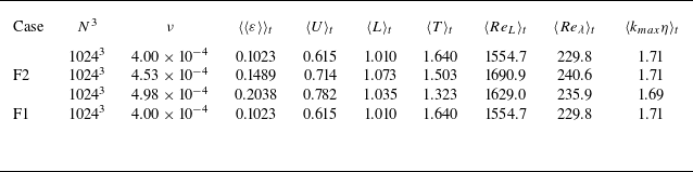
to obtain turbulence with different energy levels. The main parameters characterising the reference flows are given in table 1. All the DNS results presented in this paper are obtained with
 $N=1024$
.
Parameters of the reference flows, where
 $\langle \,\rangle$
represents spatial averaging,
 $\langle \,\rangle _{t}$
represents temporal averaging over the entire simulation time of the reference flow and
 $\langle \langle \, \rangle \rangle _{t}$
represents averaging in both space and time. Parameter
 $N^{3}$
is the number of grid points of the simulations,
 $k_{max }=N/3$
is the maximum resolvable wavenumber,
 $\nu$
is the kinematic viscosity,
 $\varepsilon$
is the dissipation and
 $\eta \equiv (\nu ^{3}/\langle \varepsilon \rangle )^{1/4}$
is the Kolmogorov scale. Velocity
 $U\equiv \sqrt {2\langle E\rangle /3}$
(where
 $E$
is the space–time local kinetic energy in the reference flow) is the root-mean-square velocity and
 $L\equiv (3\pi /4\langle E\rangle )\int k^{-1}\hat {E}(k){\rm d}k$
is the integral length scale. Time
 $T\equiv L/U$
is the large-eddy turnover time,
 ${Re}_{L}\equiv UL/\nu$
is the Reynolds number and
 ${Re}_{\lambda }\equiv Ul_{\lambda }/\nu$
is the turbulent Reynolds number defined with the Taylor length
 $l_{\lambda }\equiv \sqrt {10\langle E\rangle \nu /\langle \varepsilon \rangle }$
.

In the present work, we are mainly interested in the evolution of uncertainty without external input. To avoid external forcing effects on the uncertainty field’s evolution (see the previous section’s penultimate paragraph) we ensure that the reference and the perturbed fields are forced by the exact same forcing, i.e. that
 $\boldsymbol{g}$
vanishes. The forcing in the perturbed field is therefore determined by the velocity in the reference field, i.e.
 \begin{equation} \hat {\boldsymbol{f}}^{(2)}\left (\boldsymbol{k},t\right )=\hat {\boldsymbol{f}}^{(1)}\left (\boldsymbol{k},t\right )=\left \{\! \begin{array}{l@{\quad}l} \dfrac {\varepsilon _{0}}{2E_{f}^{(1)}}\hat {\boldsymbol{u}}^{(1)}\left (\boldsymbol{k},t\right )& \text{if } 0\lt \left |\boldsymbol{k}\right |\leqslant k_{f},\\[10pt] 0& \text{otherwise,} \end{array}\right . \end{equation}
and the uncertainty therefore grows exclusively by internal production. For consistency with our previous work (Ge et al. Reference Ge, Rolland and Vassilicos2023), we refer to this set-up as F2. To reduce statistical fluctuations, we repeat the case
 $\varepsilon _{0}=0.1$
six times, based on exactly the same reference flow (the top case in table 1), but with initial randomly generated perturbations.
To highlight the influence of external forcing on the later-time evolution of uncertainty, we simulate an additional case based on the following forcing set-up:
 \begin{equation} \hat {\boldsymbol{f}}^{(m)}\left (\boldsymbol{k},t\right )=\left \{\! \begin{array}{l@{\quad}l} \dfrac {\varepsilon _{0}}{2E_{f}^{(m)}}\hat {\boldsymbol{u}}^{(m)}\left (\boldsymbol{k},t\right )& \text{if } 0\lt \left |\boldsymbol{k}\right |\leqslant k_{f},\\[10pt] 0& \text{otherwise,} \end{array}\right . \end{equation}
with
 $\varepsilon _{0}=0.1$
and
 $m=1,2$
. In this set-up, which we refer to as F1, the external forcing applied to the reference and perturbed fields depends on the respective fields and therefore eventually grows to be different in the two fields. This case represents the configuration that has widely been applied in previous works (Boffetta & Musacchio Reference Boffetta and Musacchio2017; Mohan, Fitzsimmons & Moser Reference Mohan, Fitzsimmons and Moser2017; Berera & Ho Reference Berera and Ho2018; Ho, Armua & Berera Reference Ho, Armua and Berera2020; Ge et al. Reference Ge, Rolland and Vassilicos2023).
5. Direct numerical simulation results
In this section we present our DNS results starting with the time evolution of single-point uncertainty in § 5.1 followed by the study of the scale-by-scale uncertainty budget in § 5.2. In § 5.3 we summarise the previous subsection’s results and present a dual cascades of uncertainty hypothesis. Finally in § 5.4 we use our DNS to investigate the uncertainty production and dissipation scalings.
5.1. Time evolution of single-point uncertainty
5.1.1. Average uncertainty energy
Time evolutions of average uncertainty energy for F2 cases. For
 $\varepsilon _{0}=0.1$
,
 $\langle E_{\unicode{x1D6E5} }\rangle$
is also averaged over an ensemble of six independent realisations, while for
 $\varepsilon _{0}=0.15$
and
 $0.2$
,
 $\langle E_{\unicode{x1D6E5} }\rangle$
is only taken from a single realisation. The fluctuations of the uncertainty energy for
 $\varepsilon _{0}=0.1$
within one standard deviation from the mean are represented by the shaded area. Subfigure in bottom right: the initial time (
 $\tau \in [0,1.0]$
) growth of average uncertainty energy in semilogarithmic plot. Subfigure in top right: the uncertainty evolution during
 $\tau \in [1.0,5.0]$
, where the exponential of exponential function fit is indicated by a solid black line.

Figure 2 shows the time evolutions of
 $\langle E_{\unicode{x1D6E5} }\rangle $
for each F2 case. For
 $\varepsilon _{0}=0.1$
,
 $\langle E_{\unicode{x1D6E5} }\rangle $
is averaged over an ensemble of six independent realisations, as mentioned in § 4, while for
 $\varepsilon _{0}=0.15$
and
 $0.2$
,
 $\langle E_{\unicode{x1D6E5} }\rangle $
is only taken from a single realisation. Term
 $\langle E_{\unicode{x1D6E5} }\rangle $
decreases immediately after the perturbations are seeded because average dissipation
 $\langle \varepsilon _{\unicode{x1D6E5} }\rangle $
initially overwhelms average production
 $\langle P_{\unicode{x1D6E5} }\rangle $
in (1.1) as already observed and explained in Ge et al. (Reference Ge, Rolland and Vassilicos2023). The initial decrease regime is followed by exponential growth of
 $\langle E_{\unicode{x1D6E5} }\rangle $
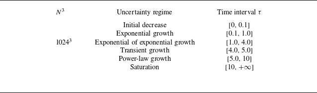
as shown in the bottom right plot of figure 2. This is the self-similar chaotic regime of uncertainty growth studied in detail by Ge et al. (Reference Ge, Rolland and Vassilicos2023). As time proceeds, the exponential growth of uncertainty energy transits into the exponential of exponential growth regime identified in Ge et al. (Reference Ge, Rolland and Vassilicos2023), as shown in the top right plot of figure 2. The time ranges for each one of these regimes are given in table 2 in terms of normalised time
 $\tau \equiv t/\,\langle T^{(1)}\rangle _{t}$
(
 $T^{(1)}$
is
 $T$
in table 1) with origin
 $\tau =0$
when the high-wavenumber small perturbation is introduced into the flow. Note that the time ranges are the same for all three F2 cases even though they have different levels of turbulence dissipation and turbulence intensity. As shown by Ge et al. (Reference Ge, Rolland and Vassilicos2023) these three time ranges are longer (shorter) in terms of normalised time
 $\tau$
for lower (higher) Reynolds numbers.
Time ranges of different uncertainty evolution regimes.

In the present work, we are particularly interested in the growth of uncertainty after the exponential of exponential growth regime which ends at about
 $\tau =4$
and before the saturation time when the uncertainty energy stops growing any further because the reference and perturbed fields have decorrelated as much as they can. It is within this time range that we may find the stochastic time range where
 $\langle E_{\unicode{x1D6E5} }\rangle $
and
 $l_{\unicode{x1D6E5} }$
both grow as power laws of time. We have run three F2 simulations with three different values of
 $\varepsilon _0$
until
 $\tau$
is close to 16 (not shown here) and have established that the saturation time is at about
 $\tau =10$
(see table 2). We therefore run the remaining five F2 simulations for
 $\varepsilon = 0.1$
until
 $\tau =11$
(see left-hand plot in figure 2) and look for power-law behaviours in the time range between
 $\tau = 4.0$
and
 $\tau =10$
. We have two alternative predictions for
 $\langle E_{\unicode{x1D6E5} }\rangle $
:
 $\langle E_{\unicode{x1D6E5} }\rangle \sim \varepsilon t$
on the basis of scalings (3.5a
)–(3.5b
) and
 $\langle E_{\unicode{x1D6E5} }\rangle \sim (\varepsilon U^{(1)} t)^{2/3}$
on the basis of scalings (3.6a
)–(3.6b
). Note that these power-law predictions are equivalent to
 $\langle E_{\unicode{x1D6E5} }\rangle /\,\langle E_{tot}\rangle \sim \tau$
and
 $\langle E_{\unicode{x1D6E5} }\rangle /\,\langle E_{tot}\rangle \sim \tau ^{2/3}$
, respectively, on account of
 $\varepsilon \sim U^{(1)3}/L^{(1)}$
. Therefore, the collapse of the three different curves in figure 2 does not favour any of the two power laws. To evaluate which power-law scaling better describes the uncertainty growth, we apply power-law fits to the time evolution of
 $\langle E_{\unicode{x1D6E5} }\rangle $
and also use finite-size Lyapunov exponent (FSLE) analysis following Boffetta et al. (Reference Boffetta, Cencini, Falcioni and Vulpiani2002).
Taking into account the translation and offset caused by the transition between different growth regimes, the applied curve fitting models are
 $a(\tau -b)+c$
(linear) and
 $a(\tau -b)^{2/3}+c$
(
 $2/3$
power law). As shown by the coefficients of determination in figure 3, a
 $2/3$
power-law fit over the time range
 $\tau _s \leqslant \tau \leqslant 10$
is rather better than a linear fit over this time range for any
 $\tau _s$
between 4 and 5 and for all three F2 cases with different turbulence and intensity levels. However, this conclusion may be contingent on the choice of time range and/or forcing configuration. We therefore now try the F1 forcing set-up and also the FSLE approach.
Coefficients
 $R^{2}$
from curve-fitting models
 $a(\tau -b)+c$
and
 $a(\tau -b)^{2/3}+c$
for the evolution of
 $\langle E_{\unicode{x1D6E5} }\rangle$
in figure 2 over the time interval
 $\tau \in [\tau _{s}, 10]$
.

Figure 4(a) compares the uncertainty energy evolutions for the F1 and F2 set-ups, both with
 $\varepsilon _{0}=0.1$
. Although there is only one single realisation for F1 and six realisations for F2, it is clearly observed that F1 significantly and systematically deviates from F2 starting from
 $\tau$
between
 $4$
and
 $5$
, which corresponds to the start of the power-law growth fitted for F2 in the previous paragraph. Linear growth of uncertainty energy has been reported in previous works for F1 in the stochastic time regime (Leith & Kraichnan Reference Leith and Kraichnan1972; Boffetta & Musacchio Reference Boffetta and Musacchio2017; Ge et al. Reference Ge, Rolland and Vassilicos2023). Therefore, this systematic deviation between F1 and F2 may indicate the critical role of external input and the possibility of a new uncertainty scaling in the stochastic time regime. Indeed, we already made the point in § 3 that different correlations between reference and uncertainty fields can, in principle, lead to different scalings.
For an additional and perhaps less ambiguous quantification of the stochastic time regime’s power law, we now use the FSLE (Boffetta et al. Reference Boffetta, Cencini, Falcioni and Vulpiani2002) defined as
 \begin{equation} \gamma _{E}(\langle E_{\unicode{x1D6E5} }\rangle )=\frac {1}{\,\langle T_{a}\rangle _{e}}\,\left \langle \ln \left (\frac {\,\langle E_{\unicode{x1D6E5} }\rangle (t+T_{a})}{\,\langle E_{\unicode{x1D6E5} }\rangle (t)}\right )\right \rangle _{e}\!, \end{equation}
where
 $\langle \,\boldsymbol\cdot\, \rangle _{e}$
denotes the ensemble average. For case F1, only a single realisation is available, so no ensemble averaging is applied. For case F2, the ensemble average is performed over six independent realisations. Time
 $T_{a}$
is the time required for
 $\langle E_{\unicode{x1D6E5} }\rangle $
to grow by a factor
 $a$
. Here, we set
 $a=2$
for
 $\langle E_{\unicode{x1D6E5} }\rangle /\,\langle E_{tot}\rangle \leqslant 0.2$
, and for larger uncertainty energies we take
 $T_a$
constant and equal to the
 $T_a$
which corresponds to
 $\langle E_{\unicode{x1D6E5} }\rangle /\,\langle E_{tot}\rangle =0.2$
. (Other choices of
 $a$
and
 $T_a$
were also tried without a change in our conclusions.) The two candidate scalings
 $\langle E_{\unicode{x1D6E5} }\rangle \sim \varepsilon t$
and
 $\langle E_{\unicode{x1D6E5} }\rangle \sim (\varepsilon U^{(1)} t)^{2/3}$
lead to
 $\gamma _{E}(\langle E_{\unicode{x1D6E5} }\rangle )\sim \varepsilon \,\langle E_{\unicode{x1D6E5} }\rangle ^{-1}$
and
 $\gamma _{E}(\langle E_{\unicode{x1D6E5} }\rangle )\sim \varepsilon U^{(1)}\,\langle E_{\unicode{x1D6E5} }\rangle ^{-3/2}$
, respectively. Figure 4(b) shows the evolution of
 $\gamma _{E}$
as a function of
 $\langle E_{\unicode{x1D6E5} }\rangle $
in cases F1 with
 $\varepsilon _{0}=0.1$
(average over one realisation) and F2 with
 $\varepsilon _{0}=0.1$
(average over six realisations). The stochastic time range deviation between F1 and F2 appears clearly in the figure, with the former following
 $\gamma _{E}(\langle E_{\unicode{x1D6E5} }\rangle )\sim \,\langle E_{\unicode{x1D6E5} }\rangle ^{-1}$
and the latter following
 $\gamma _{E}(\langle E_{\unicode{x1D6E5} }\rangle )\sim \,\langle E_{\unicode{x1D6E5} }\rangle ^{-3/2}$
.
Both the direct power-law fits of
 $\langle E_{\unicode{x1D6E5} }\rangle (\tau )$
and the FSLE analysis show that 2/3 power law better describes the stochastic time growth of uncertainty without forcing-generated uncertainty. This may also suggest an indirect preference of our F2 data for the uncertainty dissipation scalings (3.6a
)–(3.6b
) rather than (3.5a
)–(3.5b
), a point to which we return in § 5.4.
(a) Evolution of uncertainty energy for cases F1 and F2 with
 $\varepsilon _{0}=0.1$
. (b) Evolution of FSLE for cases F1 and F2 with
 $\varepsilon _{0}=0.1$
.

5.1.2. Characteristic length of uncertainty
Deciding between
 $\langle E_{\unicode{x1D6E5} }\rangle /\,\langle E_{tot}\rangle \sim \tau$
and
 $\langle E_{\unicode{x1D6E5} }\rangle /\,\langle E_{tot}\rangle \sim \tau ^{2/3}$
is more convincing if the data also favour the consistent time dependence of
 $l_{\unicode{x1D6E5} }$
in the same time range, i.e.
 $l_{\unicode{x1D6E5} }\sim \varepsilon ^{1/2} t^{3/2}$
in the case of linear time dependence of
 $\langle E_{\unicode{x1D6E5} }\rangle $
and
 $l_{\unicode{x1D6E5} }\sim U^{(1)} t$
in the case of
 $2/3$
power-law time dependence of
 $\langle E_{\unicode{x1D6E5} }\rangle $
.
Time evolution of
 $l_{\unicode{x1D6E5} }/L^{(1)}$
for F2 cases. Inset: time evolution of
 $l_{\unicode{x1D6E5} }/l_{\lambda }^{(1)}$
. For
 $\varepsilon _{0}=0.1$
,
 $l_{\unicode{x1D6E5} }$
is averaged over an ensemble of six independent realisations, while for
 $\varepsilon _{0}=0.15$
and
 $0.2$
,
 $l_{\unicode{x1D6E5} }$
is only taken from a single realisation. The fluctuations of
 $l_{\unicode{x1D6E5} }$
for
 $\varepsilon _{0}=0.1$
within one standard deviation from the mean are represented by the shaded area. Note that the two power-law predictions for
 $l_{\unicode{x1D6E5} }$
are equivalent to
 $l_{\unicode{x1D6E5} }/l_{\lambda }^{(1)}\sim \tau ^{3/2}\sqrt {U^{(1)}L^{(1)}/\nu }$
and
 $l_{\unicode{x1D6E5} }/l_{\lambda }^{(1)}\sim \tau \sqrt {U^{(1)}L^{(1)}/\nu }$
on account of
 $\varepsilon \sim U^{(1)3}/L^{(1)}$
. The three different F2 cases have more or less the same Reynolds number.

Figure 5 shows the time evolution of
 $l_{\unicode{x1D6E5} }$
for each of the F2 cases. In this figure,
 $l_{\unicode{x1D6E5} }$
is normalised by the reference field’s integral length scale
 $L^{(1)}$
, as well as the Taylor length
 $l_{\lambda }^{(1)}$
of the reference flow in order to easily check whether
 $l_{\unicode{x1D6E5} }$
is sufficiently larger than
 $l_{\lambda }^{(1)}$
during the power-law time range as this is a condition for the validity of the equilibrium model of uncertainty growth on which the power-law predictions are based.
The evolution of
 $l_{\unicode{x1D6E5} }$
, in particular during the early time when the chaoticity dominates the growth of uncertainty, has been already discussed in our previous work (Ge et al. Reference Ge, Rolland and Vassilicos2023): at the very initial times when uncertainty dissipates,
 $l_{\unicode{x1D6E5} }$
is correspondingly increasing until the chaotic regime (from
 $\tau \approx 0.1$
to
 $\tau \approx 1.0$
in the present simulations) where
 $\langle E_{\unicode{x1D6E5} }\rangle $
grows exponentially and
 $l_{\unicode{x1D6E5} }$
reaches a constant plateau as shown by Ge et al. (Reference Ge, Rolland and Vassilicos2023). After the chaotic exponential growth of
 $\langle E_{\unicode{x1D6E5} }\rangle $
,
 $l_{\unicode{x1D6E5} }$
increases again. At
 $\tau \approx 4.0$
, close to the start of the power-law regime according to our previous subsection’s results on
 $\langle E_{\unicode{x1D6E5} }\rangle $
,
 $l_{\unicode{x1D6E5} }/l^{(1)}_{\lambda }$
has reached a value of approximately
 $1.5$
(see figure 5). We may therefore consider that the decorrelation process has entered an inertial-range stochastic regime during which
 $l_{\unicode{x1D6E5} }/l^{(1)}_{\lambda }$
grows even further as a power law to reach about 4.5 at approximate saturation time
 $\tau =10$
after which
 $l_{\unicode{x1D6E5} }/l^{(1)}_{\lambda }$
oscillates around the same value for all three F2 cases. The coefficients of determination in figure 6 suggest that
 $l_{\unicode{x1D6E5} }/L^{(1)}(\tau )$
is marginally better fitted by a linear function of
 $\tau$
than by a 2/3 power law over the time range
 $\tau _s \leqslant \tau \leqslant 10$
, for any
 $\tau _s$
between 4 and 5 and for all three F2 cases in spite of their different turbulence dissipation and intensity levels. Similar to § 5.1.1, the applied curve-fitting models are
 $a(\tau -b)^{2/3}+c$
(
 $2/3$
power law) and
 $a(\tau -b)+c$
(linear) to adapt the translation and offset caused by the transition between different growth regimes.
Figure 7(a
) compares
 $l_{\unicode{x1D6E5} }$
growths and FSLEs for
 $l_{\unicode{x1D6E5} }$
for F1 and F2 with
 $\varepsilon _{0}=0.1$
in both cases. The deviation between F1 and F2 is once again observed to happen at
 $\tau$
between
 $4$
and
 $5$
. We define the FSLE for
 $l_{\unicode{x1D6E5} }$
as
 \begin{equation} \gamma _{l}(l_{\unicode{x1D6E5} })=\frac {1}{\,\langle T_{a}\rangle _{e}}\,\left \langle \ln \left (\frac { l_{\unicode{x1D6E5} }(t+T_{a})}{ l_{\unicode{x1D6E5} }(t)}\right )\right \rangle _{e}\!. \end{equation}
Here
 $a$
is set to be
 $2$
when
 $ l_{\unicode{x1D6E5} }/ l_{\unicode{x1D6E5} }^{(1)}\leqslant 1$
. When
 $l_{\unicode{x1D6E5} }/ l_{\unicode{x1D6E5} }^{(1)}\gt 1$
,
 $T_{a}$
is taken as a constant and equal to the value of
 $T_{a}$
for
 $l_{\unicode{x1D6E5} }/ l_{\unicode{x1D6E5} }^{(1)}=1$
. The two candidate scalings
 $l_{\unicode{x1D6E5} } \sim t^{3/2}$
and
 $l_{\unicode{x1D6E5} } \sim t$
yield
 $\gamma _{l}(l_{\unicode{x1D6E5} })\sim l_{\unicode{x1D6E5} }^{-2/3}$
and
 $\gamma _{l}(l_{\unicode{x1D6E5} })\sim l_{\unicode{x1D6E5} }^{-1}$
, respectively. Figure 7(b) shows the evolution of
 $\gamma _{l}$
as a function of
 $l_{\unicode{x1D6E5} }$
in case F1 (
 $\varepsilon _{0}=0.1$
and average over one realisation) and F2 with
 $\varepsilon _{0}=0.1$
(average over six realisations). The results suggest that
 $l_{\unicode{x1D6E5} }$
follows
 $\gamma _{l}(l_{\unicode{x1D6E5} })\sim l_{\unicode{x1D6E5} }^{-2/3}$
for F1 but follows
 $\gamma _{l}(l_{\unicode{x1D6E5} })\sim l_{\unicode{x1D6E5} }^{-1}$
for F2. A coherent picture of a power-law time range is therefore emerging where
 $l_{\unicode{x1D6E5} } \sim t$
and
 $\langle E_{\unicode{x1D6E5} }\rangle \sim t^{2/3}$
are both better supported by our data than
 $l_{\unicode{x1D6E5} } \sim t^{3/2}$
and
 $\langle E_{\unicode{x1D6E5} }\rangle \sim t$
for the stochastic time regime of uncertainty growth without forcing-generated uncertainty.
Coefficients
 $R^{2}$
from curve-fitting models
 $a(\tau -b)+c$
and
 $a(\tau -b)^{3/2}+c$
for the evolution of
 $l_{\unicode{x1D6E5} }$
in figure 5 over the time interval
 $\tau \in [\tau _{s}, 10]$
.

(a) Evolution of
 $l_{\unicode{x1D6E5} }$
for cases F1 and F2 with
 $\varepsilon _{0}=0.1$
. (b) Evolution of FSLE for cases F1 and F2 with
 $\varepsilon _{0}=0.1$
.

Time evolutions of ratio
 $\langle P_{\unicode{x1D6E5} }\rangle /\langle \varepsilon _{\unicode{x1D6E5} }\rangle$
for F2 cases. For
 $\varepsilon _{0}=0.1$
, ensemble averaging over six realisations is applied, whereas for the other two values of
 $\varepsilon _0$
, the data are taken from one single realisation.

5.1.3. Ratio between uncertainty production and dissipation
We close § 5.1 by addressing the proportionality between
 $\langle P_{\unicode{x1D6E5} }\rangle $
and
 $\langle \varepsilon _{\unicode{x1D6E5} }\rangle $
which is assumed in the argument of § 3. Ge et al. (Reference Ge, Rolland and Vassilicos2023) have shown a quasi-time-constant ratio
 $\langle P_{\unicode{x1D6E5} }\rangle /\,\langle \varepsilon _{\unicode{x1D6E5} }\rangle $
during time ranges which may be interpreted as stochastic time ranges in
 $N=512$
cases. Figure 8 shows the time evolutions of ratio
 $\langle P_{\unicode{x1D6E5} }\rangle /\,\langle \varepsilon _{\unicode{x1D6E5} }\rangle $
for our three F2 cases. It is observed that the ratio oscillates around a certain value, which may be considered statistically steady, in the stochastic time range
 $5\leqslant \tau \leqslant 10$
. For the case where
 $\varepsilon _{0}=0.10$
, this ensemble-averaged value is measured to be
 $1.17\pm 0.08$
, which is more stable than the other cases because of the ensemble average. This may be why the case
 $\varepsilon _{0}=0.10$
returns a better fit to the theoretical predictions than the other two cases. For the cases where
 $\varepsilon _{0}=0.15$
and
 $\varepsilon _{0}=0.20$
, the time average of the ratio during the stochastic time range, as well as its corresponding standard deviation, is
 $1.19\pm 0.16$
and
 $1.15\pm 0.11$
, respectively. Our DNS therefore supports the proportionality between
 $\langle P_{\unicode{x1D6E5} }\rangle $
and
 $\langle \varepsilon _{\unicode{x1D6E5} }\rangle $
in the stochastic time range.
For case F2 and
 $\varepsilon _{0}=0.1$
, the scale evolutions of each sphere-area-averaged term in (2.11) at different times corresponding to different uncertainty growth regimes. The Kolmogorov scale
 $\eta ^{(1)}$
, Taylor scale
 $l_{\lambda }^{(1)}$
and integral length scale
 $L^{(1)}$
are plotted as dash-dotted, dashed and solid lines, respectively. Averaging includes ensemble averaging over six realisations in all statistics plotted here.

5.2. Scale-by-scale uncertainty energy budget
The dependence on scale
 $r$
of each term in (2.11) at different times, including the time derivative of the uncertainty’s second-order structure function
 $\partial \,\langle \mathcal{A}_{\delta }^{a}\rangle /\partial t$
obtained directly from the DNS, is presented in figure 9. All these terms are averaged over the surface of a sphere of radius
 $r= \vert \boldsymbol{r}\vert$
. We have adopted this strategy as it is numerically much cheaper than evaluating every term in (2.12) by integrating over the volume of a sphere of radius
 $r$
for various
 $r$
and times
 $t$
. We only present the ensemble-averaged terms obtained for case F2 with
 $\varepsilon _{0}=0.1$
, but results for the other two F2 cases are qualitatively identical albeit with some quantitative differences which have no bearing on the conclusions and statements made in this subsection and paper in general. We checked that the sphere-area-averaged
 $\partial \,\langle \mathcal{A}_{\delta }\rangle /\partial t$
agrees well with its value obtained from the sphere-area-averaged (2.11) for all F2 cases, all
 $r$
and all times tried; see examples in figure 9. Furthermore, at
 $r=0$
the viscous diffusion term
 $\langle \mathcal{D}_{\delta }\rangle $
equals
 $\langle \varepsilon _{\unicode{x1D6E5} }\rangle $
and the interscale transfer rate
 $\langle \mathcal{I}_{\delta \uparrow }\rangle $
equals
 $-\,\langle P_{\unicode{x1D6E5} }\rangle $
at all times (see figure 9) and in all cases as required by theory (see § 2.3).
Dependence of the spatially averaged eigenvalues of
 $\boldsymbol{\Xi }^{(1)}$
and
 $\boldsymbol{\Xi }_{\unicode{x1D6E5} }$
on scale
 $r$
for three different times at the start, middle and end of the power-law growth regime. For reasons to do with computational expense, here and in figures 11 and 12,
 $\boldsymbol{r}=r \boldsymbol{e}_{x}$
where
 $\boldsymbol{e}_{x}$
is the unit vector of one of the three orthonormal directions of the simulation field.

Figure 9 presents four plots, each one corresponding to a different time: a time within the chaotic exponential growth regime, a time within the exponential of exponential growth regime, an early time and a late time within the stochastic power-law growth regime. The first major observation is that the interscale transfer rate
 $\langle \mathcal{I}_{\delta \uparrow }\rangle $
makes the largest absolute magnitude contribution to the right hand side of the sphere-area-averaged (2.11) at all times for
 $r\lt l_{\unicode{x1D6E5} }$
. It is negative at all scales
 $r$
and therefore, as explained in § 2.3, represents inverse interscale transfer caused by compression overwhelming stretching contributions to
 $\langle \mathcal{I}_{\delta \uparrow }\rangle $
. Whilst the average eigenvalues of the reference field’s relative deformation rate tensor
 $\boldsymbol{\Xi }^{(1)}$
take positive, zero and negative values and sum up to zero at all
 $r$
as predicted in § 2.3 (see figure 10
a), the two-point uncertainty half-sum velocity
 $\overline {\boldsymbol{w}}$
is predominantly aligned with the compressive eigenvector of the reference field’s relative deformation rate tensor (see figure 11
b). This preferential alignment significantly contributes to the negative sign of the sphere-area-averaged
 $\langle \mathcal{I}_{\delta \uparrow }\rangle $
; see (2.21a
). As argued in § 2.3,
 $\langle \mathcal{I}_{\delta \uparrow }\rangle $
represents the principal mechanism whereby uncertainty energy produced locally in
 $\boldsymbol{X}$
-space by compressions of the reference field’s local strain rate tensor is transferred to larger scales, and it does so by compressive motions of the reference field’s relative deformation rate tensor
 $\boldsymbol{\Xi }^{(1)}$
. Note the source of uncertainty energy transfer at
 $r=0$
,
 $\langle \mathcal{I}_{\delta \uparrow }\rangle =-\,\langle P_{\unicode{x1D6E5} }\rangle $
.
The second major observation is that the interscale transfer rates
 $\langle \mathcal{I}_{\delta \downarrow }\rangle $
and
 $\langle \Pi _{\delta ,{\textit{ref}}}\rangle $
are both positive at all times and for all accessible scales
 $r$
(figure 9), except at
 $r=0$
where they vanish. These interscale transfer rates therefore represent forward interscale transfers also caused by compression overwhelming stretching contributions as explained in § 2.3. Compressive motions are therefore responsible for both the inverse transfer by
 $\langle \mathcal{I}_{\delta \uparrow }\rangle $
and the forward transfers by
 $\langle \mathcal{I}_{\delta \downarrow }\rangle $
and
 $\langle \Pi _{\delta ,{\textit{ref}}}\rangle $
. A contributor to the compressive effect on
 $\langle \mathcal{I}_{\delta \downarrow }\rangle $
, as shown by (2.21b
), is the preferential alignment of the two-point uncertainty half-difference velocity
 $\delta {\boldsymbol{w}}$
with the compressive eigenvector of the reference field’s relative deformation tensor
 $\boldsymbol{\Xi }^{(1)}$
, which is marginally the case compared with the alignment with this tensor’s stretching eigenvector as shown in figure 11(a). The forward interscale transfer rates
 $\langle \mathcal{I}_{\delta \downarrow }\rangle $
and
 $\langle \Pi _{\delta ,{\textit{ref}}}\rangle $
are compression-driven primarily (in fact completely in the case of
 $\langle \Pi _{\delta ,{\textit{ref}}}\rangle $
; see (2.20)) because the moduli of
 $\delta {\boldsymbol w}$
and of its projections on the compressive and stretching eigenvectors are preferentially correlated with compressive rather than stretching eigenvalues of the reference field’s relative deformation tensor
 $\boldsymbol{\Xi }^{(1)}$
(see (2.20) and (2.21b
)).
Evolution of the spatially averaged alignment of (a)
 $\delta \boldsymbol{w}$
and (b)
 $\overline {\boldsymbol{w}}$
with
 $\boldsymbol{\Xi }^{(1)}$
, and (c) the spatially averaged alignment of
 $\delta \boldsymbol{w}$
with
 $\boldsymbol{\Xi }_{\unicode{x1D6E5} }$
in scale
 $r$
and time. For the definition of
 $r$
in this plot, see the caption of figure 10.

At the scale
 $r=l_{\unicode{x1D6E5} }$
, the probability distribution function of the alignment coefficient for (a)
 $|\boldsymbol{e}^{(1)}_{i}\,\boldsymbol\cdot\, \delta \boldsymbol{w}|^{2}/|\delta \boldsymbol{w}|^{2}$
, (b)
 $|\boldsymbol{e}^{(1)}_{i}\,\boldsymbol\cdot\, \overline {\boldsymbol{w}}|^{2}/|\overline {\boldsymbol{w}}|^{2}$
and (c)
 $|\boldsymbol{e}_{\unicode{x1D6E5} i}\,\boldsymbol\cdot\, \delta \boldsymbol{w}|^{2}/|\delta \boldsymbol{w}|^{2}$
at different time. For the definition of
 $r$
in this plot, see the caption of figure 10.

The one remaining interscale transfer rate is that for the nonlinear interscale transfer fully within the uncertainty field, i.e.
 $\langle \Pi _{\delta ,{\textit{err}}}\rangle $
. As can be seen in figure 9,
 $\langle \Pi _{\delta ,{\textit{err}}}\rangle $
is negative and is hardly detectable except towards the end of the power-law regime. It therefore corresponds to an inverse nonlinear interscale transfer driven by stretching motions as explained in § 2.3. Equation (2.23) shows that the effects of stretching/compressive motions on
 $\langle \Pi _{\delta ,{\textit{err}}}\rangle $
occur via the eigenvalues of
 $\boldsymbol{\Xi }_{\unicode{x1D6E5} }$
(the uncertainty field’s relative deformation rate) and the alignments of
 $\delta {\boldsymbol w}$
with the eigenvectors of
 $\boldsymbol{\Xi }_{\unicode{x1D6E5} }$
. These alignments are presented in figure 11(c) which shows that all the uncertainty energy aligns with both
 $\boldsymbol{e}_{\unicode{x1D6E5} 1}$
and
 $\boldsymbol{e}_{\unicode{x1D6E5} 3}$
. There is only a very slight preference for alignment with the stretching direction, which is hardly visible in the probability distributions of the alignments of uncertainty energy to
 $\boldsymbol{e}_{\unicode{x1D6E5} 1}$
and
 $\boldsymbol{e}_{\unicode{x1D6E5} 3}$
in figure 12(c), which actually appear to collapse throughout the stochastic time range. This slight preference results in
 $\langle \Pi _{\delta ,{\textit{ref}}}\rangle $
being less than zero, though small, if not negligible, compared with the three other interscale transfer rates.
Looking now at the evolution through the different time regimes in figure 9, we note that
 $\langle \mathcal{I}_{\delta \downarrow }\rangle $
,
 $\langle \Pi _{\delta ,{\textit{ref}}}\rangle $
and
 $-\,\langle \Pi _{\delta ,{\textit{err}}}\rangle $
grow gradually over time. Their contributions are small and may be considered negligible during the chaotic exponential growth regime, so that
 $\langle \mathcal{I}_{\delta \uparrow }\rangle $
dominates interscale transfers at scales
 $r\lt l_{\unicode{x1D6E5} }$
. In this regime,
 $\partial \,\langle \mathcal{A}_{\delta }\rangle /\partial t$
is significantly non-zero at
 $r$
values above the Kolmogorov length. At scales below
 $l_{\unicode{x1D6E5} }$
this time derivative is determined mainly by the competing influences of molecular diffusion minus dissipation
 $\langle \mathcal{D}_{\delta }\rangle - \,\langle \varepsilon _{\unicode{x1D6E5} }\rangle $
which causes
 $\langle \mathcal{A}_{\delta }\rangle $
to decrease and interscale transfer rate plus production
 $\langle \mathcal{I}_{\delta \uparrow }\rangle + \,\langle P_{\unicode{x1D6E5} }\rangle $
which causes it to increase. At scales
 $l_{\unicode{x1D6E5} }$
and larger, molecular diffusion is effectively zero and all interscale transfers are between small and negligible which is consistent with the fact, shown by Ge et al. (Reference Ge, Rolland and Vassilicos2023), that
 $l_{\unicode{x1D6E5} }$
remains approximately constant during the chaotic exponential growth regime.
After the exponential growth of
 $\langle E_{\unicode{x1D6E5} }\rangle $
, the interscale transfer rates
 $\langle \mathcal{I}_{\delta \uparrow }\rangle $
and
 $\langle \mathcal{I}_{\delta \downarrow }\rangle $
are no longer negligible at any
 $r$
between
 $l_{\unicode{x1D6E5} }$
and
 $2l_{\unicode{x1D6E5} }$
, as shown in figure 9(b–d), with
 $|\,\langle \mathcal{I}_{\delta \uparrow }\rangle (l_{\unicode{x1D6E5} }) |\gt |\,\langle \mathcal{I}_{\delta \downarrow }\rangle (l_{\unicode{x1D6E5} })|$
, suggesting that uncertainty energy is transported across
 $l_{\unicode{x1D6E5} }$
to larger scales, thereby resulting in growth of
 $l_{\unicode{x1D6E5} }$
. The time derivative of the uncertainty structure function
 $\langle \mathcal{A}_{\delta }\rangle $
remains non-negligible at all scales during the exponential of exponential growth regime, as shown in figure 9(b).
In the power-law growth regime, however, there appears a clear tendency for
 $\partial \,\langle \mathcal{A}_{\delta }\rangle /\partial t$
to approach zero for all
 $r$
smaller than
 $l_{\unicode{x1D6E5} }$
as time increases (see figure 9
c,d), thereby supporting the equilibrium
 $\partial \,\langle \mathcal{A}_{\delta }\rangle /\partial t\approx 0$
on which the equilibrium model of uncertainty growth is built in § 3. This tendency towards equilibrium at scales
 $r$
below
 $l_{\unicode{x1D6E5} }$
and the fact that viscous diffusion
 $\langle \mathcal{D}_{\delta }\rangle $
is negligible at scales
 $r\gt l_{\lambda }^{(1)}$
(see figure 9
c,d) support the prediction made in § 3 of a self-similar equilibrium cascade in the uncertainty field, and (3.4) in particular, in the range
 $l_{\lambda }^{(1)}\lt r\lt l_{\unicode{x1D6E5} }$
during the power-law growth regime.
We close this subsection with some observations about the eigenvalues/eigenvectors of
 $\boldsymbol{\Xi }^{(1)}$
and
 $\boldsymbol{\Xi }_{\unicode{x1D6E5} }$
. Figure 10 illustrates the dependence on scale and time of the spatially averaged eigenvalues of
 $\boldsymbol{\Xi }^{(1)}$
and
 $\boldsymbol{\Xi }_{\unicode{x1D6E5} }$
normalised by the spatially averaged modulus of the single-point strain rate tensor (only one single realisation of
 $\varepsilon _{0}=0.1$
, but results hold for other realisations and the other F2 cases). In agreement with our analysis in § 2.3, both
 $\boldsymbol{\Xi }^{(1)}$
and
 $\boldsymbol{\Xi }_{\unicode{x1D6E5} }$
have only two non-zero eigenvalues and their spatial averages sum up to zero. Our DNS data reveal that these spatial averages decrease with increasing scale and are approximately statistically stationary in time. Figures 11(a) and 11(b) depict the spatial alignments of
 $\delta \boldsymbol{w}$
and
 $\overline {\boldsymbol{w}}$
with the eigenvectors of
 $\boldsymbol{\Xi }^{(1)}$
for various scales and times (also one single realisation of
 $\varepsilon _{0}=0.1$
). We observe that these spatially averaged alignments remain quasi-constant across scales. A significant portion of the uncertainty energy is consistently aligned with the compression direction across both small and large scales, throughout all observed times. Additionally, figures 12(a) and 12(b) demonstrate that whereas weak alignments of the uncertainty field with the compression and stretching direction of
 $\boldsymbol{\Xi }^{(1)}$
are comparably probable, strong alignments of the uncertainty field with the compression direction of
 $\boldsymbol{\Xi }^{(1)}$
are significantly more probable than strong alignments of the uncertainty field with the stretching direction of
 $\boldsymbol{\Xi }^{(1)}$
.
5.3. Dual-cascades hypothesis
We summarise the main results of the previous subsection. Local one-point compressions of the reference field’s strain rate tensor enhance uncertainty by a production mechanism described by Ge et al. (Reference Ge, Rolland and Vassilicos2023). Then, compressive motions of the reference field’s relative deformation rate tensor generate an inverse cascade based on their interactions with the uncertainty half-sum velocity field which transfers uncertainty energy from zero length scales
 $r$
to larger ones (average interscale transfer rate
 $\langle \mathcal{I}^{a}_{\delta \uparrow }\rangle $
). These compressive motions also interact with the uncertainty half-difference velocity field to generate a forward cascade which transfers energy from large to small scales (average interscale transfer rates
 $\langle \mathcal{I}^{a}_{\delta \downarrow }\rangle $
and
 $\langle \Pi ^{a}_{\delta ,{\textit{ref}}}\rangle $
). This forward-transferred uncertainty energy originates from the forcing input rate, if there is one, and from the uncertainty production-driven inverse cascade. There is also nonlinear interscale transfer which is fully within the uncertainty field and operates independently from the reference field by uncertainty field stretching actions which generate a very slow inverse cascade (very small negative average interscale transfer rate
 $\langle \Pi ^{a}_{\delta ,{\textit{err}}}\rangle $
). In total,
 $\langle \mathcal{I}^{a}_{\delta \uparrow }\rangle $
dominates and the interscale transfer is overall inverse with uncertainty energy going from small to large scales, reflecting the dominance of uncertainty production over uncertainty dissipation. Note that at scales
 $r$
larger than
 $l_{\unicode{x1D6E5} }$
the two weakest interscale transfer rates,
 $\langle \Pi _{\delta ,{\textit{ref}}}\rangle $
and
 $\langle \Pi _{\delta ,{\textit{err}}}\rangle $
, quickly attenuate to near-zero values compared with
 $\langle \mathcal{I}_{\delta \downarrow }\rangle $
and
 $\langle \mathcal{I}_{\delta \uparrow }\rangle $
. This summary is schematically represented in figure 13.
Qualitative schematic plot for the uncertainty transfer in scales.

During the stochastic power-law growth regime, the interscale transfers are in equilibrium at scales
 $r$
smaller than
 $l_{\unicode{x1D6E5} }$
and viscous diffusion is negligible at scales
 $r$
larger than
 $l_{\lambda }^{(1)}$
, giving rise to the self-similar equilibrium cascade represented by the balance (3.4) in the inertial range
 $l_{\lambda }^{(1)} \lt r \lt l_{\unicode{x1D6E5} }$
. It is natural to ask whether this self-similar equilibrium cascade consists of two separate-on-average cascades in this scale range, one forward, driven by uncertainty dissipation and represented by the balance
 \begin{equation} \,\langle \varepsilon _{\unicode{x1D6E5} }\rangle \approx \big\langle \Pi ^{a}_{\delta ,{\textit{ref}}}\big\rangle + \big\langle \mathcal{I}^{a}_{\delta \downarrow }\big\rangle \end{equation}
and one inverse, driven by uncertainty production and represented by
 \begin{equation} -\,\langle P_{\unicode{x1D6E5} }\rangle \approx \left\langle \Pi ^{a}_{\delta ,{\textit{err}}}\right\rangle + \big\langle \mathcal{I}^{a}_{\delta \uparrow }\big\rangle. \end{equation}
This is the dual-cascades hypothesis for the stochastic power-law growth regime. A look at figures 9(c) and 9(d) does not support this hypothesis since both
 $|\,\langle \Pi _{\delta ,{\textit{ref}}}\rangle +\,\langle \mathcal{I}_{\delta \downarrow }\rangle |$
and
 $ |\!\langle \mathcal{I}_{\delta \uparrow }\rangle +\,\langle \Pi _{\delta ,{\textit{err}}}\rangle |$
decrease with increasing scale in the range
 $l_{\lambda }^{(1)}\lt r\lt l_{\unicode{x1D6E5} }$
(as actually also happens in the reference field’s energy cascade; Yasuda & Vassilicos Reference Yasuda and Vassilicos2018). However, it may be that the Reynolds numbers of our DNS are not sufficiently large.
Scale evolutions of
 $\beta /\alpha$
at different times during the power-law growth regime for cases F2 with (a)
 $\varepsilon _{0}=0.1$
, (b)
 $\varepsilon _{0}=0.15$
and (c)
 $\varepsilon _{0}=0.2$
. For
 $\varepsilon _{0}=0.1$
, the data are ensemble-averaged over six realisations, whereas for the other values of
 $\varepsilon _0$
the data are taken from one single realisation. The parts of the curves within the range of
 $l_{\lambda }^{(1)}\lt r\lt l_{\unicode{x1D6E5} }$
are plotted as solid lines whereas the parts before and after this range are dotted lines.

(a) Time evolutions of
 $\langle \beta /\alpha \rangle _{r}$
and (b) its normalised standard deviation
 $\sigma _{\beta /\alpha }/\langle \beta /\alpha \rangle _{r}$
for F2 cases.

Scatter plots for (a)
 $\langle P_{\unicode{x1D6E5} }\rangle$
versus
 $\langle E_{\unicode{x1D6E5} }\rangle ^{3/2}/l_{\unicode{x1D6E5} }$
, (b)
 $\langle \varepsilon _{\unicode{x1D6E5} }\rangle$
versus
 $\langle E_{\unicode{x1D6E5} }\rangle ^{3/2}/l_{\unicode{x1D6E5} }$
, (c)
 $\langle P_{\unicode{x1D6E5} }\rangle$
versus
 $U^{(1)}\langle E_{\unicode{x1D6E5} }\rangle /l_{\unicode{x1D6E5} }$
and (d)
 $\langle \varepsilon _{\unicode{x1D6E5} }\rangle$
versus
 $U^{(1)}\langle E_{\unicode{x1D6E5} }\rangle /l_{\unicode{x1D6E5} }$
during the time range
 $\tau \in [5.0,10]$
for F2 cases, where the linear regression and its
 $R^{2}$
value of the set of points of all six cases are given. For
 $\varepsilon _{0}=0.1$
, the averaging includes ensemble averaging over six realisations, whereas for the other values of
 $\varepsilon _0$
, the data are taken from one single realisation.

We attempt an indirect examination of the dual cascades hypothesis on the basis of a necessary condition for its validity which may be valid even at Reynolds numbers where the dual-cascades hypothesis is not. This necessary but not sufficient condition for the validity of (5.3) and (5.4) in the scale range
 $l_{\lambda }^{(1)}\ll r\ll l_{\unicode{x1D6E5} }$
is that the following equality holds in that range:
 \begin{equation} \frac {\,\langle P_{\unicode{x1D6E5} }\rangle }{\,\langle \varepsilon _{\unicode{x1D6E5} }\rangle }\approx -\frac {\big\langle \Pi ^{a}_{\delta ,{\textit{err}}}\big\rangle +\big\langle \mathcal{I}^{a}_{\delta \uparrow }\big\rangle }{\big\langle \Pi ^{a}_{\delta ,{\textit{ref}}}\big\rangle +\big\langle \mathcal{I}^{a}_{\delta \downarrow }\big\rangle }. \end{equation}
We define
 \begin{equation} \alpha (t)=\,\langle P_{\unicode{x1D6E5} }\rangle /\,\langle \varepsilon _{\unicode{x1D6E5} }\rangle \;\textrm{and}\; \beta (r,t)=- \big(\big\langle \Pi ^{a}_{\delta ,{\textit{err}}}\big\rangle +\big\langle \mathcal{I}^{a}_{\delta \uparrow }\big\rangle \big)/ \big(\big\langle \Pi ^{a}_{\delta ,{\textit{ref}}}\big\rangle +\big\langle \mathcal{I}^{a}_{\delta \downarrow }\big\rangle \big) \end{equation}
and in figure 14 we plot the scale evolution of
 $\beta /\alpha$
at different times for the three F2 cases. In most cases and times, the
 $\beta /\alpha$
curve reaches an approximate constant plateau in the scale range
 $l_{\lambda }^{(1)}\lt r\lt l_{\unicode{x1D6E5} }$
with a value reasonably close to 1. To quantitatively evaluate this value, we define the average of
 $\beta /\alpha$
over the scales
 $r$
in the range
 $1.5l_{\lambda }^{(1)}\lt r\lt 0.7l_{\unicode{x1D6E5} }$
and denote it
 $\langle \beta /\alpha \rangle _{r}$
. We present its time evolution in figure 15(a). In all three F2 DNS cases,
 $\langle \beta /\alpha \rangle _{r}$
appears statistically stationary around a time-average value
 $\langle \,\langle \beta /\alpha \rangle _{r}\rangle _{\tau }=1.05\pm 0.03$
,
 $1.03\pm 0.07$
and
 $1.05\pm 0.05$
for the cases
 $\varepsilon _{0}=0.10$
,
 $0.15$
and
 $0.20$
, respectively (
 $\langle \,\boldsymbol\cdot\, \rangle _{\tau }$
represents the time average within
 $\tau \in [5.0,10.5]$
). The standard deviation of
 $\langle \beta /\alpha \rangle _{r}$
, defined as
 \begin{equation} \sigma _{\beta /\alpha }(\tau )=\sqrt {({1}/{(0.7l_{\unicode{x1D6E5} }-1.5l_{\lambda }^{(1)})})\int _{r=1.5l_{\lambda }^{(1)}}^{0.7l_{\unicode{x1D6E5} }} (\beta /\alpha (r,\tau )-\,\langle \beta /\alpha \rangle _{r}(\tau ) )^{2}{\kern1.5pt}\mathrm{d}r}, \end{equation}
is plotted in figure 15(b), where it can be seen that it is smaller than
 $4\,\%$
of
 $\langle \beta /\alpha \rangle _{r}$
for all three cases and all times. (Note that the
 $\varepsilon _{0}=0.1$
case exhibits the most stable plateau value close to
 $1$
, presumably because it has been ensemble-averaged.) Whereas we are not able with our DNS to validate the dual-cascade hypothesis, our DNS does permit us to validate its necessary condition (5.5).
5.4. Uncertainty production and dissipation scalings
An underpinning of the uncertainty production and dissipation scalings in § 3 is the self-similar equilibrium cascade represented by the balance (3.4). Having found support for the self-similar equilibrium cascade in the range
 $l_{\lambda }^{(1)}\lt r \lt l_{\unicode{x1D6E5} }$
with our DNS data in § 5.2, we now investigate the uncertainty production and dissipation scalings with these data. In § 5.1 we have concluded that our DNS coherently favour
 $l_{\unicode{x1D6E5} } \sim t$
and
 $\langle E_{\unicode{x1D6E5} }\rangle \sim t^{2/3}$
over
 $l_{\unicode{x1D6E5} } \sim t^{3/2}$
and
 $\langle E_{\unicode{x1D6E5} }\rangle \sim t$
in the power-law time range. For the picture to be truly coherent, our DNS should also favour the scalings (3.6) over the scalings (3.5) because the former imply
 $l_{\unicode{x1D6E5} } \sim t$
and
 $\langle E_{\unicode{x1D6E5} }\rangle \sim t^{2/3}$
whereas the latter imply
 $l_{\unicode{x1D6E5} } \sim t^{3/2}$
and
 $\langle E_{\unicode{x1D6E5} }\rangle \sim t$
in the power-law regime.
Figure 16 presents four scatter plots generated with data recording the evolutions in the stochastic time range
 $\tau \in [5.0,10]$
of
 $\langle P_{\unicode{x1D6E5} }\rangle $
,
 $\langle \varepsilon _{\unicode{x1D6E5} }\rangle $
,
 $\langle E_{\unicode{x1D6E5} }\rangle ^{3/2}/l_{\unicode{x1D6E5} }$
and
 $U^{(1)}\,\langle E_{\unicode{x1D6E5} }\rangle /l_{\unicode{x1D6E5} }$
across all three F2 cases. The scatter plot of
 $\langle P_{\unicode{x1D6E5} }\rangle $
and
 $\langle E_{\unicode{x1D6E5} }\rangle ^{3/2}/l_{\unicode{x1D6E5} }$
in figure 16(a) does not support the linear relation between these two quantities advocated by the scalings (3.5). On the other hand, the scatter plot of
 $\langle P_{\unicode{x1D6E5} }\rangle $
and
 $U^{(1)}\,\langle E_{\unicode{x1D6E5} }\rangle /l_{\unicode{x1D6E5} }$
in figure 16(c) does return a much better linear relation and supports the scaling
 $\langle P_{\unicode{x1D6E5} }\rangle \sim U^{(1)}\,\langle E_{\unicode{x1D6E5} }\rangle /l_{\unicode{x1D6E5} }$
in (3.6). Concerning the average uncertainty dissipation scaling, the scatter plot of
 $\langle \varepsilon _{\unicode{x1D6E5} }\rangle $
and
 $U^{(1)}\,\langle E_{\unicode{x1D6E5} }\rangle /l_{\unicode{x1D6E5} }$
in figure 16(d) exhibits a same linear relation as the scatter plot of
 $\langle \varepsilon _{\unicode{x1D6E5} }\rangle $
and
 $\langle E_{\unicode{x1D6E5} }\rangle ^{3/2}/l_{\unicode{x1D6E5} }$
in figure 16(b). All in all, our data return a coherent picture where the uncertainty production and dissipation rates follow the scalings (3.6) and the uncertainty energy and integral length grow as
 $l_{\unicode{x1D6E5} } \sim t$
and
 $\langle E_{\unicode{x1D6E5} }\rangle \sim t^{2/3}$
in the stochastic time range.
6. Conclusion
In this paper we have studied the backward contamination of uncertainty from smaller to larger scales in the inertial range of three-dimensional, incompressible and statistically stationary homogeneous/periodic turbulence where the turbulence cascade is forward. Our focus has been on the growth of uncertainty by stochasticity rather than chaoticity (Lorenz Reference Lorenz1969; Thalabard et al. Reference Thalabard, Bec and Mailybaev2020), and therefore on the power-law growth some time after the chaotic exponential growth of average uncertainty energy
 $\langle E_{\unicode{x1D6E5} }\rangle $
.
At high enough Reynolds number the external large-scale uncertainty input cannot influence the growth of uncertainty in the inertial range (
 $F_{\unicode{x1D6E5} }=0$
). The growth of
 $\langle E_{\unicode{x1D6E5} }\rangle $
is fully controlled by internal production (
 $\langle P_{\unicode{x1D6E5} }\rangle $
) and dissipation (
 $\langle \varepsilon _{\unicode{x1D6E5} }\rangle $
), according to (1.1). To investigate the interscale transport of uncertainty energy, we developed a scale-by-scale uncertainty energy budget (2.11) based on spatially averaged energy of two-point velocity half-differences
 $\langle \left |\delta \boldsymbol{w}\right |^{2}\rangle $
, and we applied it to DNS of statistically stationary periodic turbulence. While the reference turbulence is statistically stationary, the uncertainty field is not until it eventually fully decorrelates from the reference field and reaches total (i.e. maximum) uncertainty. Nevertheless, in the stochastic time range of power-law growth of uncertainty, all uncertainty field length scales between the Taylor length (above which viscous diffusion is negligible) and the uncertainty field’s integral length scale can be considered to be effectively decorrelated from the reference field and therefore statistically stationary. With their periodicity/homogeneity this implies that they are in a self-similar two-point equilibrium where the uncertainty field interscale transfer rates sum up to be independent of length scale and equal to the difference between the average uncertainty dissipation and production rates. This equilibrium cascade of decorrelation is predominantly backward whereby uncertainty produced by local strain rate compressions at zero length scale, as already demonstrated by Ge et al. (Reference Ge, Rolland and Vassilicos2023), is transferred to progressively larger scales by
 $\langle \mathcal{I}_{\delta \uparrow }\rangle $
. This transfer to larger scales happens via compressions of the reference field’s relative deformation tensor (which we can refer to as two-point compressions) and their alignments with the half-sum uncertainty field. These two-point compressions also align with the half-difference uncertainty field giving rise to positive
 $\langle \mathcal{I}_{\delta \downarrow }\rangle $
and also correlate with its local energy giving rise to positive
 $\langle \Pi _{\delta ,{\textit{ref}}}\rangle $
so as to generate a forward transfer of uncertainty from large to small scales fed by large-scale forcing input of uncertainty and/or the predominant inverse uncertainty cascade. There is also a small, negligible for most of the time, interscale transfer (
 $\langle \Pi _{\delta ,{\textit{err}}}\rangle $
) of uncertainty by and within the uncertainty field itself which is from small to large scales. Unlike the other three interscale transfer mechanisms which are linear and dominated by two-point compressions of the reference field, this one is fully nonlinear and dominated by stretching motions of the relative deformation tensor (two-point stretchings) of the uncertainty field itself when significantly non-zero.
To summarise the main points, one-point compressive motions amplify/produce uncertainty and chaoticity locally in physical space as previously demonstrated by Ge et al. (Reference Ge, Rolland and Vassilicos2023); then, during the time range of stochasticity, two-point compressions by the reference field transfer uncertainty from zero to small to larger scales predominantly via a linear inverse interscale transfer/cascade mechanism involving the uncertainty field half-sum (low-pass uncertainty field). A linear forward interscale transfer/cascade occurs concurrently via reference field two-point compressions acting on the uncertainty field half-difference (high-pass uncertainty field) and feeding the non-zero dissipation rate of uncertainty. Compressions are key to both chaoticity and stochasticity.
In the stochastic time range of power-law growth of uncertainty our DNS support the power laws
 $l_{\unicode{x1D6E5} } \sim t$
and
 $\langle E_{\unicode{x1D6E5} }\rangle \sim t^{2/3}$
when there is no forcing-generated uncertainty. These power laws are based on the uncertainty dissipation and production scalings (3.6). The difference between these scalings (3.6) and the more conventional scalings (3.5) (which lead to different power laws for
 $l_{\unicode{x1D6E5} }$
and
 $\langle E_{\unicode{x1D6E5} }\rangle $
) is rooted in a presently naive attempt to account for the effect that correlations between the reference and uncertainty fields have on these scalings. This is an important issue which requires substantial future research.
Acknowledgements
We are grateful for the access to the computing resources supported by the Zeus supercomputers (Mésocentre de Calcul Scientifique Intensif de l’Université de Lille), Cluster Austral (Centre Régional Informatique et d’Applications Numériques de Normandie) and Lantuxinsuan (Chengdu) Technology Co. Ltd. We also thank Dr Y. Ruan from Peking University and Mr X. Ge from BROAD Group for help in obtaining computational resources.
Funding
J.G. acknowledges financial support from the China Scholarship Council.
Declaration of interests
The authors report no conflict of interest.