1 Introduction
The Richtmyer–Meshkov instability (RMI) (Richtmyer Reference Richtmyer1960; Meshkov Reference Meshkov1970) occurs when a shock wave passes through the interface between two fluids of different density. The impulsive acceleration will cause the growth of any perturbations present at the interface, and the development of the resulting instability is governed by the vorticity transport equation,
 $$\begin{eqnarray}\displaystyle & \displaystyle {\displaystyle \frac{\text{D}\unicode[STIX]{x1D74E}}{\text{D}t}}={\displaystyle \frac{1}{\unicode[STIX]{x1D70C}^{2}}}\left(\unicode[STIX]{x1D735}\unicode[STIX]{x1D70C}\times \unicode[STIX]{x1D735}p\right)+\left(\unicode[STIX]{x1D74E}\boldsymbol{\cdot }\unicode[STIX]{x1D735}\right)\boldsymbol{u}-\unicode[STIX]{x1D74E}\left(\unicode[STIX]{x1D735}\boldsymbol{\cdot }\boldsymbol{u}\right)+\unicode[STIX]{x1D708}\unicode[STIX]{x1D6FB}^{2}\unicode[STIX]{x1D74E}, & \displaystyle\end{eqnarray}$$
where
 $\unicode[STIX]{x1D70C}$
is the density,
 $p$
is the pressure,
 $\unicode[STIX]{x1D708}$
is the viscosity,
 $\boldsymbol{u}\equiv (u,v,w)$
is the velocity vector and
 $\unicode[STIX]{x1D74E}\equiv \unicode[STIX]{x1D735}\times \boldsymbol{u}$
is the vorticity. The first term on the right-hand side is called the baroclinic production term, and leads to a production of vorticity when
 $\unicode[STIX]{x1D735}p\times \unicode[STIX]{x1D735}\unicode[STIX]{x1D70C}\neq 0$
. The second term on the right-hand side is the vortex stretching term; it represents the enhancement of vorticity by stretching and is only present in three-dimensional flows. Vortex stretching is the mechanism by which turbulent energy is transferred to smaller scales. The third term on the right-hand side of (1.1) is the expansion term. In an expanding flow,
 $\unicode[STIX]{x1D735}\boldsymbol{\cdot }\boldsymbol{u}>0$
, resulting in a decrease in the magnitude of vorticity, whereas if the fluid is under compression,
 $\unicode[STIX]{x1D735}\boldsymbol{\cdot }\boldsymbol{u}<0$
, and vorticity will increase. Finally, the last term on the right-hand side of the equation is the diffusion term; this term describes the effects of viscous diffusion on the vorticity distribution.
Following passage of the shock wave, the growth of perturbations on the interface is initially linear in time. As the instability develops and the amplitudes of perturbations become large (comparable to the wavelength of the perturbation), their growth becomes nonlinear, and a turbulent mixing zone develops between the two fluids at late times. This instability occurs over a large range of both time and length scales and is responsible for mixing in a wide variety of natural phenomena. At the largest of scales, the RMI presents itself during the supernova explosion of a dying star (Kane, Drake & Remington Reference Kane, Drake and Remington1999) and is responsible for the appearance of stellar core elements at earlier-than-predicted times (Arnett Reference Arnett2000). At the smallest of scales, the RMI manifests itself as a destructive mixing mechanism in inertial confinement fusion (ICF) experiments (Lindl et al. Reference Lindl, Amendt, Berger, Glendinning, Glenzer, Haan, Kauffman, Landen and Suter2004). When maintaining perfect spherical symmetry is of the upmost importance, the RMI wreaks havoc as the mechanism for mixing of the deuterium–tritium (DT) fuel and the outer ablator layer, causing contamination of the fuel source and inhibiting thermonuclear burn. Between the largest and smallest of scales, the RMI could play a crucial role in scramjet engines as this instability may enhance fuel–oxidizer mixing in supersonic combustion applications (Marble, Hendricks & Zukoski Reference Marble, Hendricks and Zukoski1987).
A theoretical prediction for the RMI was first provided in 1960 when Richtmyer (Reference Richtmyer1960) modified work by Sir G. I. Taylor (Reference Taylor1950) to describe the evolution of an impulsively accelerated interface. In particular, he replaced the constant acceleration term in Taylor’s analysis with an impulsive one. In this way, the RMI can be considered the impulsive-acceleration limit of the Rayleigh–Taylor instability (RTI); however, unlike the RTI, the interface will be RMI unstable regardless of the direction of acceleration. Early experiments were conducted by Meshkov (Reference Meshkov1970) in an effort to test if experimental data supported theory. These experiments were conducted on single-mode interfaces in a horizontal shock tube for a variety of Mach numbers as
 $M\sim 1.25{-}1.5$
, and ultimately confirmed Richtmyer’s theory. Later experiments by Andronov et al. (Reference Andronov, Bakhrakh, Meshkov, Mokhov, Nikiforov, Pevnitskii and Tolshmyakov1976) used high-speed schlieren to extend the studies to multimode interfaces using nominally flat membranes with small, random perturbations. Multimode experiments using membranes to separate gas pairs continued for decades, including the influential work of Vetter & Sturtevant (Reference Vetter and Sturtevant1995). In these studies, a nitrocellulose membrane rested on a wire mesh, separating
 $\text{SF}_{6}$
and air. This mesh had 10 mm spacing between wires, allowing for small-scale perturbations of the membrane, as well as an imposed large-scale perturbation on the order of the shock tube width. This allowed for a ‘two-scale perturbation’, that has served as the basis of a number of numerical studies. Cohen et al. (Reference Cohen, Dannevik, Dimits, Eliason, Mirin, Zhou, Porter and Woodward2002) performed numerical simulations of this work, employing simplified piecewise-parabolic method (sPPM) simulations with varying mesh sizes to explore the importance of resolution for computational results. A similar code was used by Grinstein, Gowardhan & Wachtor (Reference Grinstein, Gowardhan and Wachtor2011) at lower resolutions (up to
 $1640\times 4802$
). Hill, Pantano & Pullin (Reference Hill, Pantano and Pullin2006) used large-eddy simulations (LES) techniques with a fifth-order weighted essentially non-oscillatory (WENO) scheme. Finally, Schilling & Latini (Reference Schilling and Latini2010) used a ninth-order WENO scheme. All of these simulations showed agreement with the experimental post-reshock growth rate, which was found to be relatively insensitive to the resolution of the numerical simulations.
Eventually, experiments using membranes and schlieren imaging gave way to membraneless interfaces visualized using planar imaging techniques. These later studies were no longer reliant on integrated diagnostics nor influenced by the presence of a membrane within the flow, and more modern diagnostics used in these studies allowed for the collection of higher fidelity data. Methods used to create a membraneless interface include gas curtains (Prestridge et al. Reference Prestridge, Rightley, Vorobieff, Benjamin and Kurnit2000), retractable plates (Brouillette & Sturtevant Reference Brouillette and Sturtevant1994) and stagnation planes (Jones & Jacobs Reference Jones and Jacobs1997). The current work aims to better understand shock-induced turbulent mixing by performing hydrodynamic experiments characterizing the RMI in a shock-accelerated shear layer, as used by Weber et al. (Reference Weber, Haehn, Oakley, Rothamer and Bonazza2012, Reference Weber, Haehn, Oakley, Rothamer and Bonazza2014). The experiments detailed in the present studies allow for concentration and velocity to be obtained at the initial condition (IC) and four post-shock times (PS1-PS4) using simultaneous planar laser-induced fluorescence (PLIF) and particle image velocimetry (PIV) measurements. This technique has been used previously to extract concentration and velocity from a shocked heavy-gas curtain, and results were used to determine the effect of the initial condition on turbulent mixing (Balasubramanian, Orlicz & Prestridge Reference Balasubramanian, Orlicz and Prestridge2013), the effects of reshock (Balakumar et al. Reference Balakumar, Orlicz, Ristorcelli, Balasubramanian, Prestridge and Tomkins2012) and to give insight into the mixing transition of variable-density flows (Orlicz et al. Reference Orlicz, Balasubramanian, Vorobieff and Prestridge2015). However, while these studies employed simultaneous PIV and PLIF measurements, the aforementioned experiments are inherently different from the present work as the gas-curtain set-up provides a two-interface initial condition, which was accelerated by a shock wave with a lower Mach number than was used in the research outlined in the present work. Recent studies conducted at Georgia Institute of Technology have also utilized simultaneous PIV and PLIF to make measurements of shock-driven, variable-density flows. The work of Mohaghar et al. (Reference Mohaghar, Carter, Musci, Reilly, McFarland and Ranjan2017) focused on both single-mode and multi-mode interfaces at an inclined angle to the shock wave. These studies report many of the same turbulence quantities discussed in the present work, though the experiments at Georgia Tech employ a lower Mach number shock to accelerate the interface, as well as a gas pair yielding a lower Atwood number than was used in the experiments described in this manuscript.
This paper begins with a detailed description of the interface creation and experimental set-up in the next section. Section 3 discusses the data processing techniques used to correct PLIF images to give concentration fields, obtain velocity fields from PIV particle image pairs, match concentration and velocity fields by accounting for scaling, rotation and a two-dimensional translation, as well as decompose fields into mean and fluctuating components. Results and a discussion of field structure and distribution, mixing layer thickness, density self-correlation, energy spectra, Reynolds stresses and Reynolds number are given in § 4. Finally, the research is summarized and conclusions are highlighted in § 5.
2 Experimental set-up
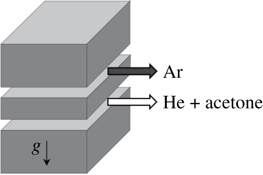
Experiments of once-shocked RMI were conducted in the Wisconsin Shock Tube Laboratory (WiSTL). This facility is equipped with a 9.13 m, vertical shock tube comprised of a circular driver section of 47 cm diameter and a square driven section with 25.4 cm sides (Anderson et al. Reference Anderson, Puranik, Oakley, Brooks and Bonazza2000). The two sections are initially separated by a 16-gauge steel diaphragm, which is burst by over-pressurizing the driver, creating a shock wave. This shock wave travels downward into the driven section where it accelerates a broadband, shear-layer interface. Embedded within the inner walls of the driven section are 12 piezoelectric pressure transducers placed along the length of the tube that are used to collect pressure readings as well as trigger the cameras and lasers used for diagnostics. A schematic of the experimental set-up used for the current studies is shown in figure 1.
Schematic of the vertical shock tube at the Wisconsin Shock Tube Laboratory showing the experimental set-up for simultaneous PIV and PLIF measurements of an impulsively accelerated interface.

Creating the initial condition used in the present work is a multi-step process. First, the driver and driven sections are evacuated to a pressure below 20 kPa in order to remove air and any other gas impurities from the shock tube. The driver section is filled to
 ${\sim}90\,\%$
of the diaphragm rupture pressure while the initial condition is created. A gravitationally stable stagnation plane is then created in the driven section by flowing a light gas (helium seeded with
 ${\sim}$
7 % acetone by volume) from the top of the tube and a heavy gas (pure argon) from the bottom while continuously evacuating excess gas through slots on the tube wall at the interface location. The flow is maintained for several minutes to ensure that all remaining air and impurities have been cleared from the tube. This gas pair has an Atwood number
 $A\equiv (\unicode[STIX]{x1D70C}_{2}-\unicode[STIX]{x1D70C}_{1})/(\unicode[STIX]{x1D70C}_{2}+\unicode[STIX]{x1D70C}_{1})=0.7$
, where
 $\unicode[STIX]{x1D70C}_{1}$
and
 $\unicode[STIX]{x1D70C}_{2}$
are the densities of the two gases. This method of creating a flat, membraneless interface is similar to that developed for the University of Arizona shock tube (Jones & Jacobs Reference Jones and Jacobs1997) and has been previously used in the WiSTL (Motl et al.
Reference Motl, Oakley, Ranjan, Weber, Anderson and Bonazza2009; Weber et al.
Reference Weber, Haehn, Oakley, Rothamer and Bonazza2012, Reference Weber, Haehn, Oakley, Rothamer and Bonazza2014; Reese et al.
Reference Reese, Oakley, Navarro-Nunez, Rothamer, Weber and Bonazza2014).
One side of the shock tube has two slots, each 3.2 mm high and separated by 12.7 mm, spanning the depth of the shock tube to allow two jets of gas to disrupt the stagnation plane. The average velocities of the jets are: argon
 $0.35~\text{m}~\text{s}^{-1}$
and He
 $+$
acetone
 $0.25~\text{m}~\text{s}^{-1}$
. The opposing side of the shock tube has a slot spanning the depth allowing the mixed gases to exit.

After the stagnation plane has stabilized, a statistically repeatable, broadband, shear-layer initial condition is set-up by injecting each gas horizontally through slots located on the shock tube side wall at the interface, 2 m above the bottom of the tube. Gas injection through the slots is sustained for the remainder of the experiment, and excess gas is continually removed by vacuum through a second set of slots on the wall opposite the gas-injection slots to maintain atmospheric pressure inside the shock tube. Details of the slot geometry and flow conditions used to establish the initial condition are given in figure 2. The light gas is flowed from the bottom set of slots while the heavy gas is flowed at a higher rate from the top set of slots; this mismatch of flowrates establishes the shear layer. The unstable density configuration used in creating the initial condition was chosen due to the more broadband generation of scales from the Rayleigh–Taylor unstable nature of the gas injection at the slots. There are a number of important properties of this interface to be considered. First, we note that this method of slot injection from the shock tube side wall creates a three-dimensional shear layer that can never be identically reproduced. However, this initial condition has been shown by Weber (Reference Weber2012) to be statistically repeatable in terms of spectral content. It also provides a reliable method of creating a membraneless interface containing a large range of scales (Weber et al. Reference Weber, Haehn, Oakley, Rothamer and Bonazza2012).
Ultraviolet light (308 nm) from a pulsed XeCl excimer laser (Lambda Physik LPX 210i;
 $430~\text{mJ}~\text{pulse}^{-1}$
) is formed into a sheet and used to excite the acetone present in the helium gas for use in planar laser-induced fluorescence (PLIF) imaging. Fluorescence from the acetone is captured on a thermoelectrically cooled (to 218 K) CCD camera (Andor model DV434-BU2), using a 50-mm Nikon lens (
 $f/1.2$
). Two filters are placed in front of the lens: a bandpass filter centred at 470 nm with a full-width half-max of 271 nm, and an ultrasteep short-pass filter only allowing passage of signal below 524 nm. This combination of filters ensures that only fluorescence signal from PLIF was captured by the Andor sensor.
For the PIV measurements,
 $\text{TiO}_{2}$
particles with a nominal diameter of 300 nm are seeded into both gas cross-flows used to create the initial condition shear interface, and into the regions immediately above and below the interface. These particles allow for the Mie scattering of the second harmonic output (532 nm) of a dual-head, flashlamp-pumped Nd:YAG laser (Ekspla model NL303D;
 $460~\text{mJ}~\text{pulse}^{-1}$
). Using a series of optics, a laser sheet is formed for use in planar laser imaging, and allows for cameras to capture particle images with a
 ${\sim}20\times 25~\text{cm}$
field of view. Post-shock image pairs are captured with a 29 MP interline image transfer camera (TSI Inc. model 630094) using a
 $4~\unicode[STIX]{x03BC}\text{s}$
inter-frame time, while initial condition image pairs are taken with the same camera, but using an inter-frame time of 1 ms. The inter-frame times are chosen to compensate for the vastly different interface velocity fluctuations before and after acceleration by the shock wave. These timings also allow for the final search box used in PIV to be reduced in order to obtain a large number of velocity vectors, yielding finer spatial resolution of velocity while maintaining sufficient displacement of the particles.
Once the shear interface has stabilized and is properly seeded with both acetone and
 $\text{TiO}_{2}$
particles, ten initial condition images are taken and a pair of fast-acting valves (FAVs) allows high pressure gas from a pair of boost tanks to enter the driver section. This driver supply gas is nitrogen for the
 $M=1.6$
case, and helium for the
 $M=2.2$
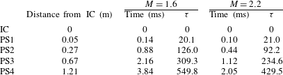
case. The over-pressurized driver causes the diaphragm to rupture, which creates the downward-travelling shock wave. Following shock acceleration of the initial condition, the interface is imaged at four different post-shock times in the development of the RMI. A summary of the post-shock locations and times (as well as non-dimensional times, see (4.4)) is given in table 1. For each Mach number, 20 experiments are conducted at every post-shock time (yielding a total of 160 post-shock data sets) to allow for ensemble averaging of results to obtain converged statistics from concentration and velocity data.
Although it would be desirable to have data at the same non-dimensional time for any
 $M$
, it would require continual optical access which is not possible for structural purposes at the reported shock strengths. Therefore, imaging is performed at discrete locations and the comparison of the two
 $M$
, either in dimensional or non-dimensional time, is not one to one. Comparing the two
 $M$
is still possible when looking at trends that evolve with time, be they integral measures such as mixing layer thickness or fluctuations relevant to turbulence. When discussing results in this paper, the notation PS1-4 will be used even though these more correctly refer to spatial locations in the shock tube relative to the initial interface position. We refer to early time, such as PS1, and late time, such as PS4, and these labels are strictly in the context of this paper and the data presented. Admittedly, particularly for numerical simulations where there is no physical limit to constrain the times when data can be taken, what is referred to in this paper as a late time behaviour (PS4) may still be considered early by other investigators and therefore the times given in table 1 should be used for objective comparison.
Summary of experimental image times and locations.

3 Data processing
3.1 Concentration from PLIF
Prior to processing the PLIF images to reveal mole fraction, the background signal is subtracted from each raw image. The background signal is an ensemble average of 10 images with the same optical setup, including laser pulses, but with no acetone in the field of view. This background image contains both the camera noise and light scattered off the walls of the shock tube. A second background subtraction step is then applied, subtracting the average intensity in the unseeded portion of the flow (i.e. the lower portion of the image). This ensures that the unseeded portion of the flow has an average intensity of zero. Analytically, this procedure is
 $$\begin{eqnarray}\displaystyle S_{i,j}^{f,temp}=I_{i,j}^{raw}-\langle I_{i,j,k}^{bg}\rangle _{k}, & & \displaystyle\end{eqnarray}$$
 $$\begin{eqnarray}\displaystyle S_{i,j}^{f}=S_{i,j}^{f,temp}-\langle S_{i,j}^{f,temp}\rangle _{i,j\in \{unseeded\}}, & & \displaystyle\end{eqnarray}$$
where angle brackets denote averaging over the subscript,
 $k$
is the background image number, unseeded is the rows and columns of the unseeded region of the image and
 $S^{\,f}$
is the final fluorescence signal. Equation (3.1) is an element-wise subtraction of a matrix and (3.2) is a subtraction of a constant value.
Next, the background-subtracted PLIF images are processed to extract the light-gas mole fraction,
 $\unicode[STIX]{x1D709}$
, by correcting for non-uniform laser profile, laser sheet divergence and Beer’s law attenuation. First, the background-subtracted PLIF image is transformed to an
 $r{-}\unicode[STIX]{x1D703}$
coordinate system aligned with the laser beam and is corrected for the signal decrease from laser sheet divergence. Then a region in the top portion of the image is selected where a uniform concentration of pure seeded (light,
 $\unicode[STIX]{x1D709}=1$
) gas exists. The Beer’s law attenuation coefficient is determined from this region, corresponding to the acetone absorption cross-section. The normalized acetone concentration can then be computed (Collins & Jacobs Reference Collins and Jacobs2002) by integrating downward while accounting for the divergence of the laser sheet, such that deviations from Beer’s law attenuation are attributed to mixing of unseeded (heavy) gas or changes in temperature. The equation for this is
 $$\begin{eqnarray}\displaystyle & \displaystyle \unicode[STIX]{x1D709}={\displaystyle \frac{\displaystyle {\displaystyle \frac{T}{T_{1}}}S^{\,f}}{\displaystyle S^{\,f,R}-n_{1}\unicode[STIX]{x1D70E}\unicode[STIX]{x1D719}\int _{r}^{R}{\displaystyle \frac{S^{\,f}}{\unicode[STIX]{x1D719}}}\,\text{d}r}}, & \displaystyle\end{eqnarray}$$
where
 $S^{\,f}$
is the local fluorescence signal,
 $S^{\,f,R}$
is the fluorescence signal at the top of the image where it is assumed
 $\unicode[STIX]{x1D709}=1$
,
 $T/T_{1}$
is the temperature ratio in relation to the pure seeded region,
 $n_{1}\unicode[STIX]{x1D70E}$
is the product of number density and absorption cross-section in the pure seeded gas (this product is measured by the exponential signal variation in the top of the image) and
 $\unicode[STIX]{x1D719}$
is the fluorescence quantum yield. The integral is carried out from the location
 $r$
to the top of the image at location
 $R$
. This process is similar to that used by Weber et al. (Reference Weber, Haehn, Oakley, Rothamer and Bonazza2014). It should be noted that temperature is approximated as
 $$\begin{eqnarray}\displaystyle & \displaystyle T=T_{2}^{\dagger }+(T_{1}^{\ddagger }-T_{2}^{\dagger })\unicode[STIX]{x1D709}, & \displaystyle\end{eqnarray}$$
where daggers (
 $\dagger$
) indicate that a region of gas has been shocked, while double daggers (
 $\ddagger$
) represent twice-shocked gas (by shock and reshock), such that
 $T_{1}^{\ddagger }$
and
 $T_{2}^{\dagger }$
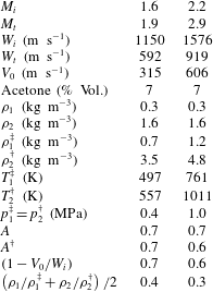
are the post-shock temperatures in the pure light and heavy gases, respectively, calculated from one-dimensional (1-D) gas dynamics. A summary of the properties of the gases used for each Mach number case in the present work is given in table 2.
Gas properties for the two Mach number cases, where daggers denote post-shock quantities. Gas 1 is the light gas (helium seeded with acetone) and gas 2 is the heavy gas (argon).

Once concentration has been determined from fluorescence signal as described in (3.3), the concentration field is then mapped back into the
 $x{-}z$
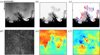
coordinate system. Finally, the 2-D Fourier transform of the corrected image is computed and the spectrum is notch filtered to remove index of refraction artefacts that appear during the image processing procedure (Weber Reference Weber2012). Following the notch filtering, the inverse transform of the corrected spectrum is computed and a final concentration field is obtained for each experiment. A representative raw PLIF image is shown in figure 3(a), and the corresponding processed image showing concentration is shown in figure 3(b). In the corrected PLIF image, white indicates pure light gas, black corresponds to pure heavy fluid and grey regions represent mixed gas of various species concentration.
3.2 Velocity from PIV
The concept behind obtaining velocity from PIV particle image pairs is simple: with a known time between images
 $\unicode[STIX]{x0394}t$
, if a group of particles from image 1 is advected to a different location in image 2 and the spatial displacement of that group of particles
 $\unicode[STIX]{x0394}\boldsymbol{x}(\boldsymbol{x},t)$
can be determined, the velocity
 $\boldsymbol{u}(\boldsymbol{x},t)$
for that small search region is estimated using
 $$\begin{eqnarray}\displaystyle & \displaystyle \boldsymbol{u}(\boldsymbol{x},t)={\displaystyle \frac{\unicode[STIX]{x0394}\boldsymbol{x}(\boldsymbol{x},t)}{\unicode[STIX]{x0394}t}}. & \displaystyle\end{eqnarray}$$
In the present experiments, the most-likely displacement vector of particle groups is determined through spatial correlation analysis of the experimental particle image pairs using the Insight 4G PIV software package from TSI Inc.
Representative data processing results and field matching for PLIF and PIV. (a) Raw fluorescence signal, (b) corrected PLIF image showing concentration with white indicating pure light gas and black corresponding to pure heavy fluid, (c) out-of-plane vorticity,
 $\unicode[STIX]{x1D714}_{y}$
, overlaid on
 $\unicode[STIX]{x1D709}$
field to show field matching, (d) raw PIV particle image, (e) output streamwise velocity with red indicating downward-moving gas and blue corresponding to upward-travelling fluid and (f) output transverse velocity with red indicating rightward-moving gas and blue corresponding to leftward-travelling fluid.

For each of the 20 concentration images obtained at every post-shock time, a corresponding particle image pair is captured by the PIV camera such that each pixel is
 ${\sim}50~\unicode[STIX]{x03BC}\text{m}$
in the focal plane. A single raw particle image is shown in figure 3(d). Similarly to processing PLIF images, the first step in obtaining velocity from PIV image pairs is subtracting the background signal from each raw image. Here the background signal for the first particle image is an ensemble average of 10 first-frame images, while the background signal for the second particle image of the pair is an ensemble average of 10 second-frame images. As with PLIF, all background images use the same optical set-up, including laser pulses, and contain both the camera noise and light scattered off the walls of the shock tube; however, no
 $\text{TiO}_{2}$
particles are present in the field of view for PIV background images. It is this background-subtracted particle image pair that is used as input to the Insight 4G PIV algorithm.
Before conducting cross-correlation, a
 $5\times 5$
Gaussian filter with
 $\unicode[STIX]{x1D70E}=0.5$
is applied to background-subtracted image pairs. Following this pre-processing step, a recursive Nyquist grid is used to break the input images into smaller spots for processing, and the first processing pass computes the vector field at a starting spot size of
 $128\times 128$
pixels with 50 % overlap grid spacing. The results of this first processing pass are then used to optimize the spot offsets for the second pass, where the spot size is reduced by a factor of two. This optimization and spot-size reduction occur once more so that a final spot size of
 $32\times 32$
pixels is achieved. At each pass, a zero pad mask is applied to compute the average pixel intensity of each spot and subtract it from each pixel prior to passing the spots to the correlation engine. This zero pad mask is chosen to increase the signal-to-noise ratio of correlations.
A direct correlator is used to compute the correlation function of the masked spots and return the result as a correlation map. The correlation is computed by first determining the mean intensity in the sample box of image 1,
 $$\begin{eqnarray}\displaystyle & \displaystyle \bar{I_{a}}={\displaystyle \frac{1}{B_{x}B_{y}}}\mathop{\sum }_{k=1}^{B_{x}}\mathop{\sum }_{l=1}^{B_{y}}I_{a}(k,l), & \displaystyle\end{eqnarray}$$
and the mean intensity of the current test box in image 2,
 $$\begin{eqnarray}\displaystyle & \displaystyle \bar{I_{b}}={\displaystyle \frac{1}{B_{x}B_{y}}}\mathop{\sum }_{k=1}^{B_{x}}\mathop{\sum }_{l=1}^{B_{y}}I_{b}(k+i,l+j), & \displaystyle\end{eqnarray}$$
where
 $I_{a}(1,1)$
and
 $I_{b}(1,1)$
represent the pixel intensities at the corner of a pattern box of size
 $B_{x}$
by
 $B_{y}$
, centred at image coordinates (
 $x,y$
), in images 1 and 2, respectively. This spot mean intensity is then subtracted from each pixel, and the product of intensities at each pixel offset is summed to give the correlation map. This correlation map is adjusted by an autocorrelation factor to increase the displacement measurement accuracy, giving the variance normalized correlation, or covariance. The highest peak in this correlation map is used to locate the particle image displacement, and is determined using a Gaussian peak engine. The Gaussian peak engine locates the correlation peak with sub-pixel accuracy by fitting a Gaussian curve to the highest pixel and its four nearest neighbours. Two 3-point fits are done: one in the
 $x$
direction with the peak pixel and the pixels to the left and right of the peak, and one in the
 $z$
direction with the peak pixel and the pixels above and below the peak. The Gaussian peak equation is given by
 $$\begin{eqnarray}\displaystyle & \displaystyle \text{d}x=x+{\displaystyle \frac{\text{log}(l)-\text{log}(r)}{2[\text{log}(l)+\text{log}(r)-2\text{log}(c)]}}-x_{0}, & \displaystyle\end{eqnarray}$$
where
 $l$
,
 $r$
, and
 $c$
are the intensity value for the left, right, and peak pixels in the correlation map,
 $x$
is the integer shift, and
 $x_{0}$
is the zero shift location. The uncertainty of the PIV measurement was quantified using the correlation statistics method (Sciacchitano et al.
Reference Sciacchitano, Neal, Smith, Warner, Vlachos, Wieneke and Scarano2015) and the
 $32\times 32$
box uncertainties in the mixing layer fit a log-normal distribution. Corresponding uncertainties from the lognormal peaks, for the low and high Mach numbers, respectively, are
 $0.62~\text{m}~\text{s}^{-1}$
and
 $0.73~\text{m}~\text{s}^{-1}$
.
With the
 $x$
and
 $z$
displacements determined by Insight, full-field transverse and streamwise velocity can be easily determined using (3.5) with the known inter-frame time between particle images. Velocity results are then post-processed to remove outliers using a global validation and a
 $5\times 5$
pixel local test to replace velocity values outside
 $3\unicode[STIX]{x1D70E}$
with the local median. Typical velocity results for the streamwise and transverse directions are shown in figure 3(e,f), respectively. Figure 3(e) shows streamwise velocity, with downward-travelling regions in red and upward-moving fluid in blue. Comparison with figure 3(b) shows that regions of upward-going gas correspond to spikes and downward-moving regions correspond to bubbles in the interface structure. Figure 3(f) shows transverse velocity, with rightward-travelling gas in red and leftward-moving fluid in blue.
3.3 Field matching
With concentration and velocity fields determined from the raw PLIF and PIV images as described in the previous two sections, the velocity results determined by Insight 4G must now be matched to the corrected
 $\unicode[STIX]{x1D709}$
field coordinate system, so as not to sacrifice the spatial resolution of the PLIF data. This is accomplished using images of a test target taken prior to each experiment by both the PLIF and PIV cameras to determine the transformation matrix
 $\unicode[STIX]{x1D64F}$
that will map the PIV target coordinates
 $(\mathfrak{x},\mathfrak{z})$
to the PLIF target (and
 $\unicode[STIX]{x1D709}$
field) coordinates
 $(x,z)$
as
 $$\begin{eqnarray}\displaystyle [x~~z~~1]=[\mathfrak{x}~~\mathfrak{z}~~1]\unicode[STIX]{x1D64F}. & & \displaystyle\end{eqnarray}$$
Because the lines of sight of both cameras are perpendicular to the imaging plane with an overlapping region of interest, the transformation to map the PIV target image to the concentration field need only include rotation, scaling, and a two-dimensional translation, such that
 $$\begin{eqnarray}\displaystyle \unicode[STIX]{x1D64F}=\left[\begin{array}{@{}ccc@{}}\mathfrak{s}\cos (\unicode[STIX]{x1D6E9}) & -\mathfrak{s}\sin (\unicode[STIX]{x1D6E9}) & 0\\ \mathfrak{ s}\sin (\unicode[STIX]{x1D6E9}) & \mathfrak{s}\cos (\unicode[STIX]{x1D6E9}) & 0\\ T_{x} & T_{z} & 1\end{array}\right], & & \displaystyle\end{eqnarray}$$
where
 $\mathfrak{s}$
is the scale factor,
 $\unicode[STIX]{x1D6E9}$
is the rotation angle,
 $T_{x}$
is the
 $x$
-direction translation and
 $T_{z}$
is the
 $z$
-direction translation. Target images are used to determine the four unknown parameters in (3.10) by selecting control points in the PLIF target image, and then selecting the corresponding points in the PIV target image to determine the geometric transformation
 $\unicode[STIX]{x1D64F}$
.
Before applying the determined transformation to velocity fields, velocity output from Insight 4G must first be resized to match the PIV target image. Since the final search box used to determine velocity from the PIV particle image pair was
 $32\times 32$
pixels with 50 % overlap, this means that for each
 $16\times 16$
pixel region in the PIV target image, there will only be a single data point in the corresponding velocity field. Hence, prior to applying
 $\unicode[STIX]{x1D64F}$
, velocity fields are first up-sampled using a bi-cubic interpolation where the output pixel value is a weighted average of pixels in the nearest
 $4\times 4$
neighbourhood. Finally, because the two cameras’ sensors had different aspect ratios, the transformed velocity field must also be cropped to the same
 $1024\times 1024$
size as the
 $\unicode[STIX]{x1D709}$
field. By cropping the transformed velocity results, each pixel in the
 $u(x,z)$
and
 $w(x,z)$
fields will match directly to a corresponding pixel in the
 $\unicode[STIX]{x1D709}(x,z)$
field.
The effectiveness of this matching technique can be seen by overlaying the transformed velocity results on the concentration field. This is demonstrated by first computing the out-of-plane vorticity (
 $\unicode[STIX]{x1D714}_{y}$
, henceforth referred to simply as
 $\unicode[STIX]{x1D714}$
) using the two known components of the velocity,
 $\unicode[STIX]{x1D74E}\equiv \unicode[STIX]{x1D735}\times \boldsymbol{u}$
, and overlaying vorticity above a certain threshold on the corresponding
 $\unicode[STIX]{x1D709}$
field, as shown in figure 3(c). Here we see that, as expected, the regions of strongest vorticity correspond directly to those locations of concentration that have the strongest gradients. Moreover, by visualizing the vorticity of the gas within the mixing zone, further insight into the effect of velocity on interface structure can be easily obtained.
3.4 Decomposition of fields
The first step in determining velocity fluctuations in the flow is to subtract the field average velocity from each pixel. For the streamwise direction, this subtraction accounts for the post-shock interface velocity, and is near the 1-D gas dynamics value of the flow (
 ${\sim}315~\text{m}~\text{s}^{-1}$
for
 $M=1.6$
, and
 ${\sim}605~\text{m}~\text{s}^{-1}$
for
 $M=2.2$
), such that
 $$\begin{eqnarray}\displaystyle {\hat{w}}=w-w_{avg}, & & \displaystyle\end{eqnarray}$$
where
 $w$
is the measured velocity field,
 $w_{avg}$
is a single value representing a global field average velocity and
 ${\hat{w}}$
is the mean-subtracted velocity field which will be referred to as the global fluctuations. This
 ${\hat{w}}$
field has a velocity distribution centred about
 $0~\text{m}~\text{s}^{-1}$
, and shows the large-scale structure of the streamwise velocity. An example of a mean-subtracted velocity field is shown in figure 4(a). The same process is also carried out for the transverse velocity field, though it should be noted that, unlike
 $w_{avg}$
, the value of
 $u_{avg}$
remains near zero for all experiments.
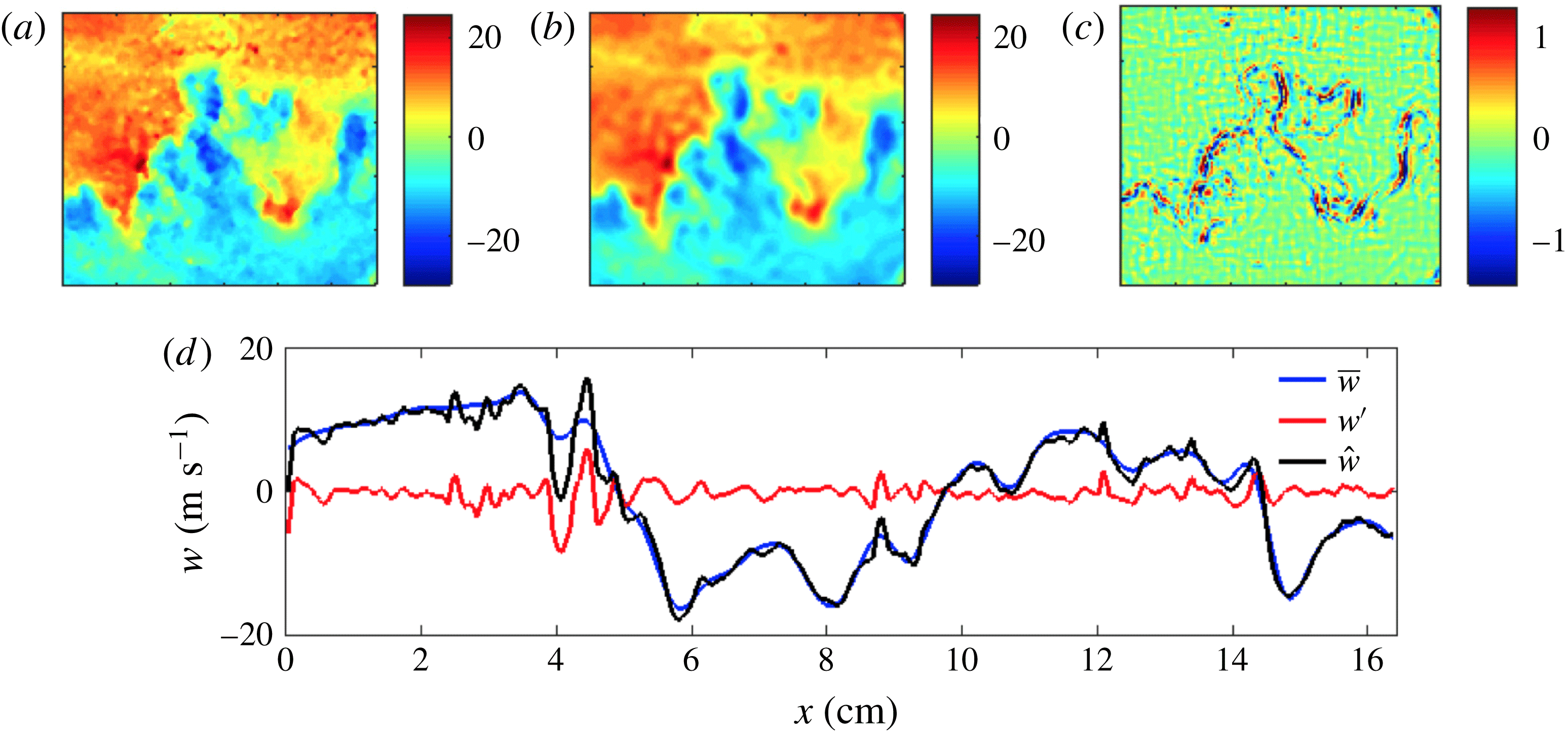
Field decomposition showing the (a) global mean-subtracted field
 ${\hat{w}}$
, (b) mean field
 $\overline{w}$
, (c) fluctuation field
 $w^{\prime }$
, and (d) line plots showing the breakdown into mean and fluctuations through the mixing layer.

With the global fluctuation fields determined from (3.11), the flow can now be further decomposed into a mean field and a local-fluctuation field. Two different methods were applied to achieve this decomposition, and each was applied to both the concentration and velocity fields so that
 $$\begin{eqnarray}\displaystyle \hat{\boldsymbol{u}}=\overline{\boldsymbol{u}}+\boldsymbol{u}^{\prime }\quad \text{and}\quad \unicode[STIX]{x1D709}=\overline{\unicode[STIX]{x1D709}}+\unicode[STIX]{x1D709}^{\prime }, & & \displaystyle\end{eqnarray}$$
where an overbar indicates the mean field and a prime denotes the fluctuating field which will be referred to as the local fluctuations. Ideally, one would ensemble average results over several experiments to obtain a mean flow field; however, the run-to-run variation of the fields proved too great to give meaningful results using this method. Instead, the first technique we will explore to determine this decomposition involves using a two-dimensional moving boxcar average to calculate a mean component of concentration and velocity for each experiment, while the second method utilizes spectral filtering to remove small-wavenumber features from the fields.
The mean flow field was first obtained for each experiment by filtering the concentration and velocity global-fluctuation fields with a 2-D moving boxcar average. Of course, since this method of filtering utilizes a set window size over which averaging occurs, the size of the filtering window should be based on some macroscopic feature of the flow to account for the growth of the mixing layer thickness over time. Here, the filter window size was chosen to be
 $1/20$
of the average height of the
 $0.05<\langle \unicode[STIX]{x1D709}\rangle <0.95$
region of the mixing layer for each post-shock time and Mach number case. In this way, as the number of pixels over which the average is being calculated increases, the boxcar average window grows proportionally. After applying this filter to the concentration and global-fluctuation velocity fields to obtain the mean component of the flow, results were subtracted from the
 $\unicode[STIX]{x1D709}$
and
 $\hat{\boldsymbol{u}}$
fields to yield the local-fluctuation fields.
A spectral method was also used to determine the decomposition of concentration and velocity fields. For this method, a two-dimensional fast Fourier transform (FFT) is performed on the field before applying a Fermi–Dirac soft cutoff filter (Heim, Jesch & Ghandhi Reference Heim, Jesch and Ghandhi2014). The kernel of the soft cutoff filter is calculated as
 $$\begin{eqnarray}\displaystyle & \displaystyle {\displaystyle \frac{1}{1+\exp \left(\displaystyle \frac{k_{xz}-k_{c}}{0.1k_{c}}\right)}}, & \displaystyle\end{eqnarray}$$
where
 $k_{xz}=\sqrt{k_{x}^{2}+k_{z}^{2}}$
is the two-dimensional wavenumber, and
 $k_{c}=(2\unicode[STIX]{x03C0})/L_{c}$
is the cutoff wavenumber with
 $L_{c}$
being the cutoff length scale. The filter gradually sets the Fourier coefficients above
 $k_{c}$
to zero. The Liepmann–Taylor scale,
 $\unicode[STIX]{x1D706}_{L}$
, defined by Grinstein (Reference Grinstein2016) as
 $\unicode[STIX]{x1D706}_{L}=2.17\unicode[STIX]{x1D706}_{T}$
(where
 $\unicode[STIX]{x1D706}_{T}$
is the Taylor microscale), makes a natural cutoff length scale as
 $\unicode[STIX]{x1D706}_{L}$
represents the smallest scale generated by the largest eddies. In other words, the Liepmann–Taylor scale bounds the isotropic region from the energy containing range (i.e. is an upper limit of the inertial range). Finally, the two-dimensional inverse fast Fourier transform (IFFT) is applied to obtain a low-pass (or spatially averaged) field. As with the moving boxcar method, this average field is subtracted from the
 $\unicode[STIX]{x1D709}$
or
 $\hat{\boldsymbol{u}}$
field to obtain the local-fluctuation field. Results using this spectral method showed good agreement with results using the boxcar method.
Field decomposition results are shown in figure 4 for the streamwise component of velocity using the spectral method of filtering. Figure 4(a) shows the
 ${\hat{w}}$
global-fluctuation field, and figures 4(b) and 4(c) show the corresponding mean
 $\overline{w}$
and local-fluctuation field
 $w^{\prime }$
, respectively. We note that figure 4(c) shows large fluctuations embedded in underlying smaller random fluctuations, and that the regions of strongest fluctuations correspond with the regions of highest vorticity, as shown in figure 3(c). A line plot from the centre row is shown in figure 4(d), where the black line shows the global fluctuation, the blue line shows the mean component of velocity, and the red line shows the local fluctuating component of the flow. We note that this methodology for obtaining local fluctuations is an advancement over techniques used in previous work where the field to be analysed is obtained by performing a columnwise subtraction of the spanwise-averaged field profile (Balakumar et al.
Reference Balakumar, Orlicz, Ristorcelli, Balasubramanian, Prestridge and Tomkins2012; Weber et al.
Reference Weber, Haehn, Oakley, Rothamer and Bonazza2014; Gerashchenko & Prestridge Reference Gerashchenko and Prestridge2015).
4 Results and discussion
4.1 Field structure and distribution
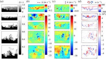
The experimental campaign discussed in this paper yielded planar concentration and two-dimensional, two-component velocity results for nearly 200 shocked interfaces; a representative subset of these fields is shown in figure 5. Figure 5(a) shows concentration results, where white corresponds to pure light gas, black corresponds to areas containing only argon and grey indicates regions of mixed fluid. Figure 5(b) shows the global-fluctuation transverse velocity field, where blue corresponds to leftward-moving gas and red indicates rightward-going fluid. Figure 5(c) shows the global fluctuation streamwise velocity field, with blue indicating upward-moving fluid and downward-travelling gas shown in red. Finally, figure 5(d) shows the vorticity field
 $\unicode[STIX]{x1D714}$
calculated from the curl of the velocity. The broadband, shear-layer initial condition is shown in the top row, and post-shock results (PS1–PS4) are shown in the following four rows. Note the difference in colour bar scaling for velocity and vorticity fields between the initial condition and post-shocked results due to the vastly different velocities within the mixing layer before and after acceleration by the shock wave.
Representative field evolution results for the
 $M=1.6$
case. From top to bottom: IC, PS1, PS2, PS3, PS4. From left to right: concentration
 $\unicode[STIX]{x1D709}$
, global-fluctuation transverse velocity
 $\hat{u}$
, global-fluctuation streamwise velocity
 ${\hat{w}}$
and vorticity
 $\unicode[STIX]{x1D714}$
.

The shear-layer initial condition
 $\unicode[STIX]{x1D709}$
-field is shown in the top row of figure 5(a), while the
 $\hat{u}$
field shows a rightward-moving jet corresponding to the injected gas from the left side of the tube, with recirculation zones developing above and below the injection site on the left side of the velocity field. The
 ${\hat{w}}$
field shows alternating upward and downward traveling gas typical of the Kelvin–Helmholtz and Rayleigh–Taylor instabilities. Due to the horizontal injection of gas used to create the shear layer, vorticity fields for the initial condition show a generally horizontal banding of vorticity across the interface. In the next row down, the PS1
 $\unicode[STIX]{x1D709}$
-field shows compression of the interface following passage of shock wave, while
 $\hat{u}$
shows the beginning of a breakup of the coherent jet seen in the initial condition and
 ${\hat{w}}$
shows an intensifying of the alternating upward and downward velocity. There is a continual breakup of the jet and a development of large-scale spike and bubble structures seen at each successive post-shock time, until coherent spike and bubble structures appear by the latest post-shock time. In the last row of figure 5, the effect of velocity on interface structure is evident as regions of strong upward motion correspond with spike features, and downward-moving gas aligns perfectly with bubbles in the
 $\unicode[STIX]{x1D709}$
-field. Vorticity is shown to be strongest along the regions of largest gradients in the
 $\unicode[STIX]{x1D709}$
-field, and the horizontal banding of
 $\unicode[STIX]{x1D714}$
seen at the initial condition has given way to alternating vertical bands of vorticity aligned with the spike and bubble structures seen at the PS4 time. While fields shown here are for
 $M=1.6$
, results are similar for the higher Mach number case, although there is more turbulent mixing occurring by late times for the
 $M=2.2$
case, as evident by the break down to smaller-scale features and more ‘grey’ mixed gas regions in the
 $\unicode[STIX]{x1D709}$
-fields. This increased mixing at higher Mach number is explored further through probability density functions (PDFs) of concentration, as well as the density self-correlation across the mixing layer as discussed in § 4.4.
The overall composition of the mixing layer (within
 $0.05<\left\langle \unicode[STIX]{x1D709}\right\rangle <0.95$
) is obtained from two-dimensional PDFs of concentration by
 $$\begin{eqnarray}\displaystyle \text{PDF}\left(\unicode[STIX]{x1D709}\right)=\int _{-0.5}^{0.5}\text{PDF}\left(\unicode[STIX]{x1D709},\tilde{z}\right)\,\text{d}\tilde{z}, & & \displaystyle\end{eqnarray}$$
where
 $\tilde{z}$
is the vertical direction scaled by the height of the
 $0.05<\left\langle \unicode[STIX]{x1D709}\right\rangle <0.95$
region of the interface. These PDFs are shown in figure 6 for the (a)
 $M=1.6$
data and (b)
 $M=2.2$
data. Had a region containing the entire interface been considered in the PDF calculation, one would expect to see an initially bimodal distribution (with the modes at
 $\unicode[STIX]{x1D709}=0$
,1) that would grow monotonically at intermediate values as the amount of mixed fluid increases at later times. However, by only considering fluid within the
 $0.05<\left\langle \unicode[STIX]{x1D709}\right\rangle <0.95$
region, the PDFs instead show that a local peak near
 $\unicode[STIX]{x1D709}\sim 0.5$
reduces over time and appears to mix with the lighter (
 $\unicode[STIX]{x1D709}=1$
) fluid. This process occurs more rapidly in the
 $M=2.2$
case and results in an increase in the fluid for
 $\unicode[STIX]{x1D709}>0.5$
. This bias for mixing of the lighter fluids has been noticed elsewhere and is attributed to the greater inertia of the heavy fluid (Livescu & Ristorcelli Reference Livescu and Ristorcelli2008; Weber et al.
Reference Weber, Haehn, Oakley, Rothamer and Bonazza2014). Figures 6(a) and 6(b) also show a nearly monotonic increase of PDF(
 $\unicode[STIX]{x1D709}$
) in time for
 $\unicode[STIX]{x1D709}=0$
and
 $\unicode[STIX]{x1D709}=1$
due to the development of spikes and bubbles in the mixing zone that cause more unmixed fluid to be brought into the
 $0.05<\left\langle \unicode[STIX]{x1D709}\right\rangle <0.95$
region as the interface becomes more distorted at late times. A rapid increase in PDF(
 $\unicode[STIX]{x1D709}$
) near
 $\unicode[STIX]{x1D709}=1$
for the
 $M=1.6$
case indicates that light gas is penetrating into the mixing layer without mixing, while the more gradual increase in PDF(
 $\unicode[STIX]{x1D709}$
) near
 $\unicode[STIX]{x1D709}=1$
for the
 $M=2.2$
case shows that, while there is a larger fraction of light fluid in the mixing layer due to bubble development, this fluid is mixing with the surrounding gas as it penetrates the interface.
Probability density functions of (a)
 $\unicode[STIX]{x1D709}$
for the
 $M=1.6$
case, (b)
 $\unicode[STIX]{x1D709}$
for the
 $M=2.2$
case, (c)
 $\hat{u}$
for the
 $M=1.6$
case, (d)
 $\hat{u}$
for the
 $M=2.2$
case, (e)
 ${\hat{w}}$
for the
 $M=1.6$
case and (f)
 ${\hat{w}}$
for the
 $M=2.2$
case. Units for
 $\hat{u}$
and
 ${\hat{w}}$
are
 $\text{m}~\text{s}^{-1}$
.

This same method of determining PDFs within the 5 %–95 % mixing region is applied to the corresponding transverse and streamwise global velocity fluctuations as well. Global velocity fluctuations in the transverse direction (shown in figures 6(c) and 6(d) for the
 $M=1.6$
and
 $M=2.2$
cases, respectively) show a dual-peaked PDF(
 $\hat{u}$
) for the initial condition. The right peak seen in the initial condition PDFs is due to the positive velocity associated with the rightward-moving injected gas jet used to set-up the shear layer, while the left peak corresponds to the distribution about the stationary
 $u=0$
gas, but has been shifted off zero by the subtraction of
 $u_{avg}$
to obtain the
 $\hat{u}$
field. Following passage of the shock wave, the velocity increases by approximately two orders of magnitude and the two peaks begin moving closer together. This convergence of peaks continues through PS2, until they have combined into a single peak by PS3 for each case. By PS4, transverse velocity again begins to develop a dual-peaked structure, likely due to the outward growth associated with expanding spikes and bubbles that have developed by this latest time.
In the streamwise direction, PDFs show (in figures 6(e) and 6(f) for the low and high Mach number cases, respectively) a nearly Gaussian distribution of velocity at the initial condition that increases by approximately three orders of magnitude following shock acceleration. The PDF distribution peaks at PS3 for the
 $M=1.6$
case and at PS2 for the
 $M=2.2$
case, and this difference could be associated with an earlier transition to turbulence for the higher Mach number case. Further evidence of this transition occurring near PS3 for the
 $M=1.6$
case and near PS2 for the
 $M=2.2$
case is presented through measurements of density self-correlation and Reynolds number in §§ 4.4 and 4.7, respectively. After reaching the peak value near
 ${\hat{w}}=0$
, the PDF(
 ${\hat{w}}$
) distribution takes on a dual-peaked structure due to the development of large-scale spikes and bubbles. This two-peaked structure of the PDFs for streamwise velocity begins sooner and shows greater spread in velocity by the latest time for the high Mach number case, though both cases show a larger peak associated with the upward-moving (
 ${\hat{w}}<0$
) spikes than for the downward-going (
 ${\hat{w}}>0$
) bubbles.
4.2 Spanwise-averaged profiles
Velocity and concentration profiles are investigated here, where the spanwise-averaged mole-fraction field is defined by
 $$\begin{eqnarray}\displaystyle & \displaystyle \left\langle \unicode[STIX]{x1D709}\right\rangle ={\displaystyle \frac{1}{x_{2}-x_{1}}}\int _{x_{1}}^{x_{2}}\unicode[STIX]{x1D709}\,\text{d}x, & \displaystyle\end{eqnarray}$$
where
 $x_{1}$
and
 $x_{2}$
are the first and last spanwise position for which
 $\unicode[STIX]{x1D709}$
measurements were obtained, respectively, such that the integral is performed across the entire width of the field for each experiment to yield a single profile. A similar approach was used for the transverse and streamwise global velocity fluctuations. The vertical coordinate of the profiles from individual experiments are each scaled by the height of the
 $0.05<\left\langle \unicode[STIX]{x1D709}\right\rangle <0.95$
region of the turbulent mixing zone (
 $h_{5{-}95}$
), where the most extreme values of
 $\left\langle \unicode[STIX]{x1D709}\right\rangle =0.05$
and
 $\left\langle \unicode[STIX]{x1D709}\right\rangle =0.95$
were chosen to yield the largest
 $h_{5{-}95}$
. Scaled profiles are then ensemble averaged to create a single profile at each time. Ensemble spanwise-averaged profiles for each post-shock time are shown in figure 7, with results for
 $M=1.6$
experiments on the left, and profiles from the
 $M=2.2$
case on the right.
Spanwise-averaged profiles of concentration and velocity for
 $M=1.6$
(a,c,e) and
 $M=2.2$
(b,d,f). From top to bottom: Concentration, global transverse velocity fluctuations and global streamwise velocity fluctuations.

Figure 7(a,b) shows the spanwise-averaged concentration results. These profiles look very different from previously reported profiles (Weber et al.
Reference Weber, Haehn, Oakley, Rothamer and Bonazza2014) despite the similarities with these earlier studies. The difference comes from the chosen match point for interface height scaling and ensemble averaging. Because each experiment produces an interface of differing thickness, when scaling by the
 $h_{5{-}95}$
and averaging results from individual runs, experiments must be matched at a chosen point. This match point will be the common location where profiles from each time will overlap, by definition. In previous experiments, the
 $\unicode[STIX]{x1D709}=0.05$
(or
 $\unicode[STIX]{x1D709}=0.95$
) locations were used as match points, and profiles showed rough, irregular slopes matched at the corresponding
 $z/h_{5{-}95}=-0.5$
(or 0.5) locations. In the present work however, a central value of
 $\unicode[STIX]{x1D709}=0.5$
was chosen as the match point. As a result, concentration results in figure 7 show more symmetric, ‘S’-shaped spanwise-averaged profiles which are centred on
 $z/h_{5{-}95}=0$
.
The initial condition concentration profile shows a gradual slope with a kink in the profile just below the
 $z/h_{5{-}95}=-1$
location. This kink should be attributed to variability in the exact location of the shear jet used in creating the initial condition interface, which is shown to be located at a similar
 $z/h_{5{-}95}$
height in the transverse velocity profiles in figure 7(c,d). After shock, this gradual slope is shown to steepen in time, with a more rapid increase occurring for the higher Mach number case. This steepening in time is a result of pure (
 $\unicode[STIX]{x1D709}=0$
or
 $\unicode[STIX]{x1D709}=1$
) gas being pushed into the mixing zone with the development of spikes and bubbles at late times. Consequently, bubbles will cause the
 $\langle \unicode[STIX]{x1D709}\rangle$
value to increase ever closer to the interface midpoint above the
 $z/h_{5{-}95}=0$
location, while spikes will drive the
 $\langle \unicode[STIX]{x1D709}\rangle$
value towards zero below the interface.
In figure 7(c,d), spanwise-averaged profiles are shown for the global transverse velocity fluctuations,
 $\hat{u}$
. These profiles show the rightward-moving jet used to establish the shear-layer initial condition occurring near
 $z/h_{5{-}95}=-0.7$
, along with recirculation zones directly above and below the jet region. These features are also clear in the initial condition transverse velocity fields shown in figure 5. Following passage of the shock wave, global transverse velocity profiles for PS1 show compression and a nearly
 $10\times$
increase in spanwise velocity. What was the central jet region is also shown to push downwards from the top of the mixing layer towards the centre of the mixing layer near
 $z/h_{5{-}95}=0$
. At higher
 $M$
acceleration there is greater compression of what was the jet region, which is also pushed deeper into the centre of the mixing layer when compared with the low
 $M$
case. The velocity in the recirculation zone above the jet remnant is accentuated as time progresses such that the entire region above the jet remnant pushes leftward at late time. Alternatively, a monotonic increase in spanwise velocity with time is observed to occur below the interface, corresponding to bulk rightward motion below the interface midpoint. This increase in spanwise-averaged global transverse velocity above and below the interface is roughly
 $3\times$
greater for the higher Mach number case than in the low Mach number experiments.
Finally, spanwise-averaged profiles of the global streamwise velocity fluctuations are shown in figure 7(e,f). While not easily seen in figure 7, the streamwise velocity in the initial condition is found to be positive above the interface and negative below it. This is due to the fact that the light gas is filled from the top of the tube and flows downward (with positive streamwise velocity), while the heavy gas is filled from the bottom of the tube and pushes upwards (with negative streamwise velocity) towards the interface. From the initial condition to PS1, velocities in the streamwise direction are shown to increase by more than two orders of magnitude. Each successive profile shows a general steepening in time, corresponding to an increase in velocity, with regions above the interface moving downwards with ever-increasing speed, and regions below the interface moving upwards increasingly rapidly. This trend is likely due to the development of the large-scale spikes and bubbles in the flow, where the light gas continues to push downwards through the interface, and the heavy gas approaches the mixing zone more readily with the development of penetrating spikes. Similar trends are observed for both the low and high Mach number cases, with slightly higher velocities by the latest time for the
 $M=2.2$
case.
4.3 Mixing-layer thickness
Mixing-layer thickness measurements. (a) Adjusted interface (bottom) eliminates additional height added by large-scale features present in the uncorrected mixing layer (top), and results in better collapse of thickness measurements. (b) Symbols show the average non-dimensional threshold measurements of the
 $0.05<\langle \unicode[STIX]{x1D709}\rangle <0.95$
region in time, error bars show the standard deviation from the 20 experiments and dotted line shows a power-law fit to data.

Threshold measurements of the
 $0.05<\langle \unicode[STIX]{x1D709}\rangle <0.95$
mixing-layer thickness,
 $h_{5{-}95}$
, are made using a spanwise-averaged mole-fraction field similar to results discussed in the previous section, but with an important adjustment made to the interface. Since better collapse of the thickness measurements was obtained by removing large-scale structures from the mixing layer, this interface adjustment is made prior to spanwise averaging the field. This is done by first finding the midpoint location between the
 $\langle \unicode[STIX]{x1D709}\rangle =0.05$
and
 $\langle \unicode[STIX]{x1D709}\rangle =0.95$
rows for each spanwise position, defined as
 $z_{0}$
and shown in figure 8(a) (top) as a red line across the mixing layer. Each spanwise position is then vertically shifted to bring all
 $z_{0}$
to the same height, as shown in figure 8(a) (bottom). If the spanwise position was shifted upwards, the bottom of that location was padded with zeros, while if the spanwise position was moved downwards, the top was filled with ones.
From the adjusted interface, threshold measurements of
 $h_{5{-}95}$
were obtained for each experiment and averaged to give a single thickness measurement at every post-shock time. Results were non-dimensionalized using
 $h_{0}^{\ast }$
– the pre-shock interface thickness scaled by the compression factor
 $(1-V_{0}/W_{i})$
– and the dominant wavenumber,
 $$\begin{eqnarray}\displaystyle \hbar =(h_{5{-}95}-h_{0}^{\ast })k_{0}, & & \displaystyle\end{eqnarray}$$
and time was non-dimensionalized as,
 $$\begin{eqnarray}\displaystyle \unicode[STIX]{x1D70F}=tV_{0}A^{+}h_{0}^{\ast }k_{0}^{2}, & & \displaystyle\end{eqnarray}$$
where
 $t$
is the time,
 $V_{0}$
is the post-shock interface velocity,
 $W_{i}$
is the incident shock-wave speed,
 $A^{+}$
is the post-shock Atwood number and
 $k_{0}$
is the dominant wavenumber. The value for
 $k_{0}$
is determined from the initial conditions as
 $k_{0}=2\unicode[STIX]{x03C0}/\unicode[STIX]{x1D706}_{0}$
, where
 $\unicode[STIX]{x1D706}_{0}$
is the dominant wavelength, similarly to the method used by Weber (Reference Weber2012). These non-dimensional thickness measurements are shown in figure 8(b), where error bars show the standard deviation from the 20 experiments at each time, and the dotted line shows a power-law fit to data such that
 $$\begin{eqnarray}\displaystyle (h_{5{-}95}-h_{0}^{\ast })k_{0}=a(tV_{0}A^{+}h_{0}^{\ast }k_{0}^{2})^{\unicode[STIX]{x1D703}}, & & \displaystyle\end{eqnarray}$$
where
 $a$
is unity and the power-law fits
 $\unicode[STIX]{x1D703}=0.34\pm 0.01$
. This value of
 $\unicode[STIX]{x1D703}$
is similar to previously reported values (
 $0.25\leqslant \unicode[STIX]{x1D703}\leqslant 0.5$
) in the work of Dimonte & Schneider (Reference Dimonte and Schneider1997, Reference Dimonte and Schneider2000), Prasad et al. (Reference Prasad, Rasheed, Kumar and Sturtevant2000), Jacobs et al. (Reference Jacobs, Krivets, Tsiklashvili and Likhachev2013) and Weber et al. (Reference Weber, Haehn, Oakley, Rothamer and Bonazza2014).
Comparison of mixing-layer thickness definitions showing that integral measurements are proportional to threshold measurements of thickness.

A similar measure of the mixing-layer thickness, called the mixing product thickness,
 $h_{p}$
, can be obtained from the adjusted spanwise-averaged profiles. This has been used previously by Cook & Dimotakis (Reference Cook and Dimotakis2001) and Weber et al. (Reference Weber, Haehn, Oakley, Rothamer and Bonazza2014), and is defined as
 $$\begin{eqnarray}\displaystyle & \displaystyle h_{p}=\int _{-\infty }^{\infty }\unicode[STIX]{x1D709}_{p}\left(\left\langle \unicode[STIX]{x1D709}\right\rangle \right)\,\text{d}z, & \displaystyle\end{eqnarray}$$
where
 $$\begin{eqnarray}\displaystyle \unicode[STIX]{x1D709}_{p}(\unicode[STIX]{x1D709})=\left\{\begin{array}{@{}ll@{}}2\unicode[STIX]{x1D709}\quad & \text{for }\unicode[STIX]{x1D709}\leqslant 0.5\\ 2(1-\unicode[STIX]{x1D709})\quad & \text{for }\unicode[STIX]{x1D709}>0.5,\end{array}\right. & & \displaystyle\end{eqnarray}$$
is the mixture composition, and an equimolar mixture has
 $\unicode[STIX]{x1D709}_{p}=1$
. This quantity is shown in figure 9 and these integral measurements of thickness are found to be proportional to the threshold measurement
 $h_{5{-}95}$
value (
 $h_{p}=0.57h_{5{-}95}$
). This proportionality is identical to measurements made by Weber et al. (Reference Weber, Haehn, Oakley, Rothamer and Bonazza2014), despite the different growth exponent
 $\unicode[STIX]{x1D703}$
due to the adjustment used to remove large-scale features from the interface.
The threshold and integral measurements of the mixing-layer thickness explored above do not differentiate between mixed gas and gas that is penetrating the interface but remains unmixed. For this, a definition of ‘mixedness’ will need to be introduced. The relative amount of molecular mixing occurring within the interface can be characterized as a ratio of a mixing length to an entrainment length. Multiple definitions have been proposed, but perhaps the two most commonly referenced global mixing parameters are those by Youngs (Reference Youngs1994):
 $$\begin{eqnarray}\displaystyle & \displaystyle \unicode[STIX]{x1D6E9}={\displaystyle \frac{\displaystyle \int _{-\infty }^{\infty }\langle \unicode[STIX]{x1D709}(1-\unicode[STIX]{x1D709})\rangle \,\text{d}z}{\displaystyle \int _{-\infty }^{\infty }\langle \unicode[STIX]{x1D709}\rangle \langle 1-\unicode[STIX]{x1D709}\rangle \,\text{d}z}}, & \displaystyle\end{eqnarray}$$
and a similar definition by Cook & Dimotakis (Reference Cook and Dimotakis2001):
 $$\begin{eqnarray}\displaystyle & \displaystyle \unicode[STIX]{x1D6EF}={\displaystyle \frac{\displaystyle \int _{-\infty }^{\infty }\langle \unicode[STIX]{x1D709}_{p}\rangle \,\text{d}z}{h_{p}}}. & \displaystyle\end{eqnarray}$$
For both cases, a ratio with a value of 1 corresponds to a fully homogenized fluid without interpenetrating perturbations, while a value of 0 indicates no molecular mixing of the fluids. It should be noted that the terms
 $\unicode[STIX]{x1D709}_{p}$
(in
 $\unicode[STIX]{x1D6EF}$
) and
 $\unicode[STIX]{x1D709}(1-\unicode[STIX]{x1D709})$
(in
 $\unicode[STIX]{x1D6E9}$
) both have the property of being maximal for
 $\unicode[STIX]{x1D709}=0.5$
and decrease monotonically toward
 $\unicode[STIX]{x1D709}=0,1$
. The two definitions of mixedness were compared in Cook, Cabot & Miller (Reference Cook, Cabot and Miller2004) and Mellado, Sarkar & Zhou (Reference Mellado, Sarkar and Zhou2005) and were shown to give very similar results. This similarity between the two definitions of global mixing is also seen in the current studies. The latter definition was used by Weber et al. (Reference Weber, Haehn, Oakley, Rothamer and Bonazza2014), and produced results comparable to those found for
 $\unicode[STIX]{x1D6EF}$
in the present work.
As shown in figure 10, the value of both
 $\unicode[STIX]{x1D6E9}$
and
 $\unicode[STIX]{x1D6EF}$
is found to strictly decrease in time for the low
 $M$
case, and decrease before increasing again for the high
 $M$
case. Youngs’ definition of mixedness is larger than Cook’s definition during compression, while the opposite is true at late times. This is a similar trend to what has been previously reported, where
 $\unicode[STIX]{x1D6E9}$
underpredicts the initial homogenization of fluid and then also underpredicts the ensuing fluid mixing at later times when compared to
 $\unicode[STIX]{x1D6EF}$
values of mixedness. Measurements of
 $\unicode[STIX]{x1D6EF}$
show that for both values of
 $M$
, it reaches a final value near 0.8, which is the asymptotic value reported after the onset of turbulent mixing in Rayleigh–Taylor simulations (Cook et al.
Reference Cook, Cabot and Miller2004), while
 $\unicode[STIX]{x1D6E9}$
approaches a value slightly below 0.8. Simulations have also shown that the cross from
 $\unicode[STIX]{x1D6E9}$
over-predicting to under-predicting the mixed fluid measurement (when compared with
 $\unicode[STIX]{x1D6EF}$
values of mixedness) occurs following the rapid growth of
 $\unicode[STIX]{x1D6E9}$
and
 $\unicode[STIX]{x1D6EF}$
that occurs after reaching the minimum value. This could be used to argue that, like the
 $M=2.2$
case, the
 $M=1.6$
value for
 $\unicode[STIX]{x1D6E9}$
and
 $\unicode[STIX]{x1D6EF}$
could also decrease between PS1 and PS2 before increasing again at later times; however, this effect is not captured at the times the interface was studied in this work.
Comparison of mixing definitions
 $\unicode[STIX]{x1D6EF}$
and
 $\unicode[STIX]{x1D6E9}$
for the low and high Mach number experiments.

4.4 Density self-correlation
The density self-correlation (DSC) is another measure of fluid mixing, where a value of zero indicates perfectly mixed fluid. Density self-correlation is an important quantity for turbulence modelling and appears in the production term of the mass-flux equation. Previous experiments have measured DSC to provide validation for initializing the BHR (Besnard–Harlow–Rauenzahn) RANS (Reynolds-averaged Navier Stokes) model (Orlicz et al. Reference Orlicz, Balasubramanian, Vorobieff and Prestridge2015) for variable density flows. DSC is involved in the conversion of potential energy into kinetic energy, and is defined by
 $$\begin{eqnarray}\displaystyle & \displaystyle b=-\left\langle \unicode[STIX]{x1D70C}^{\prime }\left({\displaystyle \frac{1}{\unicode[STIX]{x1D70C}}}\right)^{\prime }\right\rangle , & \displaystyle\end{eqnarray}$$
where brackets denote spanwise averaging and primes indicate fluctuations. The DSC is determined by first calculating density from the measured concentration field using
 $$\begin{eqnarray}\displaystyle \unicode[STIX]{x1D70C}=\unicode[STIX]{x1D70C}_{2}^{\dagger }+(\unicode[STIX]{x1D70C}_{1}^{\ddagger }-\unicode[STIX]{x1D70C}_{2}^{\dagger })\unicode[STIX]{x1D709}, & & \displaystyle\end{eqnarray}$$
where a single dagger indicates once-shocked gas, a double dagger represents twice-shocked gas (by the incident and reflected shock wave) and
 $\unicode[STIX]{x1D70C}_{1}$
and
 $\unicode[STIX]{x1D70C}_{2}$
are the density of the light and heavy gases, respectively. The fluctuating component of the density field and
 $1/\unicode[STIX]{x1D70C}$
is then determined using the spectral filtering method described in § 3.4. While the correlation is between the density field and its reciprocal, the means and other moments of
 $\unicode[STIX]{x1D70C}$
and
 $1/\unicode[STIX]{x1D70C}$
will generally not be related by reciprocals.
Average density self-correlation measurements for the (a)
 $M=1.6$
case and (b)
 $M=2.2$
case. Example of ensemble averaging over 20 experiments to obtain mean
 $b$
measurements shown in (c), where coloured lines show data from individual experiments and the black line shows the campaign average. Details of the
 $\unicode[STIX]{x1D709}$
field showing evidence of mixing differences at the latest post-shock time for the (d) low Mach number, and (e) high Mach number cases.

The mean value of DSC as a function of height through the mixing layer is shown in figure 11(a) for the
 $M=1.6$
case and in figure 11(b) for the
 $M=2.2$
case. Results were obtained by ensemble averaging the 20 DSC measurements from individual experiments to obtain a mean value for every post-shock time at each Mach number. This averaging technique is shown in figure 11(c), where the coloured lines show density self-correlation measurements for individual experiments, while the thick black line shows the average DSC profile for that post-shock time.
Measurements of the DSC through the mixing layer for the low Mach number case show general growth in time, indicating that the fluid is less mixed at later times. This is likely the result of large spikes and bubbles carrying unmixed fluid into the mixing layer. However, for the high Mach number case, DSC measurements show growth through PS2, before decaying at PS3 and PS4. The turnaround in the DSC trend for the
 $M=2.2$
case is caused by the increased mixing and breakdown to smaller scales associated with a transition to turbulence. This difference in the behaviour of the DSC between the low and high Mach number cases can be better understood by a comparison of the
 $\unicode[STIX]{x1D709}$
(and ultimately
 $\unicode[STIX]{x1D70C}$
) fields at the latest post-shock time. Figure 11(d) shows a bubble and spike that have developed at PS4 for the
 $M=1.6$
case, showing the largely unmixed fluid penetrating the mixing layer leading to an increase in DSC. Conversely, figure 11(e) shows a similar feature for the
 $M=2.2$
case, where the spike and bubble have smaller-scale features and increased mixing (more grey regions within the mixing layer) relative to the low Mach number case, leading to a reduction of the DSC mixing measurement at late times. This evidence of transition to turbulence occurring by PS2 for the
 $M=2.2$
case is further supported by Reynolds number measurements discussed in § 4.7.
4.5 Energy spectra
The scale dependence of concentration and velocity fluctuations is reported here using one-dimensional energy spectra. This approach has been applied previously for variable-density turbulence in the Rayleigh–Taylor instability (Dalziel, Linden & Youngs Reference Dalziel, Linden and Youngs1999; Wilson & Andrews Reference Wilson and Andrews2002; Ramaprabhu & Andrews Reference Ramaprabhu and Andrews2004; Mueschke, Andrews & Schilling Reference Mueschke, Andrews and Schilling2006; Banerjee, Kraft & Andrews Reference Banerjee, Kraft and Andrews2010), as well as shocked gas-curtain experiments (Vorobieff, Rightley & Benjamin Reference Vorobieff, Rightley and Benjamin1998; Vorobieff et al.
Reference Vorobieff, Mohamed, Tomkins, Goodenough, Marr-Lyon and Benjamin2003) and shear-layer interface experiments (Weber et al.
Reference Weber, Haehn, Oakley, Rothamer and Bonazza2014), which have reported the existence of a
 $k^{-5/3}$
inertial range. These experiments showing a
 $k^{-5/3}$
scaling in the inertial range are corroborated by simulations (Miles et al.
Reference Miles, Blue, Edwards, Greenough, Hansen, Robey, Drake, Kuranz and Leibrandt2005; Hill et al.
Reference Hill, Pantano and Pullin2006; Schilling & Latini Reference Schilling and Latini2010), while other simulations found
 $k^{-3/2}$
to fit better at late times (Thornber et al.
Reference Thornber, Drikakis, Youngs and Williams2010), and others still found turbulence spectra that did not scale well with either
 $k^{-5/3}$
or
 $k^{-3/2}$
(Cohen et al.
Reference Cohen, Dannevik, Dimits, Eliason, Mirin, Zhou, Porter and Woodward2002; Grinstein et al.
Reference Grinstein, Gowardhan and Wachtor2011). Zhou (Reference Zhou2001) has suggested that the spectrum of RMI turbulence should scale as
 $k^{-3/2}$
in the inertial range before reducing to the classical Kolmogorov
 $k^{-5/3}$
scaling at late times.
One-dimensional scalar power spectra,
 $E_{\unicode[STIX]{x1D709}}(k_{x})$
, are computed in the self-similar (horizontal) direction within the region
 $0.05<\left\langle \unicode[STIX]{x1D709}\right\rangle <0.95$
and results are averaged over rows from all 20 experiments at each post-shock time. To reduce the influence of noise and extend the spectrum at the highest wavenumbers, an interlacing technique is used (Kaiser & Frank Reference Kaiser and Frank2007; Weber et al.
Reference Weber, Haehn, Oakley, Rothamer and Bonazza2014) where the Fourier coefficient,
 $F(\unicode[STIX]{x1D709}(x))$
, is multiplied by the complex conjugate of the Fourier coefficient of the adjacent row,
 $$\begin{eqnarray}\displaystyle E_{\unicode[STIX]{x1D709}}(k_{x})\approx F(\unicode[STIX]{x1D709}_{j}(x))F^{\ast }(\unicode[STIX]{x1D709}_{j+1}(x)). & & \displaystyle\end{eqnarray}$$
This averaged, interlaced scalar power spectrum is shown in figures 12(a) and 12(b) for the low and high Mach number cases, respectively. All spectra have been normalized by their peak value for a better comparison of relative energy distribution in time. While spectra appear to tend towards a
 $k^{-5/3}$
inertial range by the latest time for both Mach numbers, this slope is only achieved at the lowest wavenumbers near
 $k_{x}\simeq 100~\text{m}^{-1}$
before dropping off at higher wavenumbers. Comparison of figures 12(a) and 12(b) show that, for the high Mach number case, spectra approach their late time form slightly more quickly than for the low Mach number case. The cutoff wavelength for PLIF is based on the laser sheet thickness and corresponds to a cutoff wavenumber of
 $1.8\times 10^{4}~\text{m}^{-1}$
. For PIV, the overlap size of 16 pixels is used as the cutoff wavelength and corresponds to a cutoff wavenumber of
 $1.08\times 10^{4}~\text{m}^{-1}$
.
A similar approach was taken to obtain the turbulent kinetic energy (TKE) spectra. Since only two components of velocity were measured, we will refer to these spectra as planar TKE. Because these flows are variable density, it is necessary to consider both density and velocity when calculating TKE. As with the scalar power spectra, the planar TKE spectrum is calculated using the interlacing method,
 $$\begin{eqnarray}\displaystyle \text{TKE}(k_{x})\approx F({\mathcal{K}}_{j}(x))F^{\ast }({\mathcal{K}}_{j+1}(x)), & & \displaystyle\end{eqnarray}$$
where
 ${\mathcal{K}}$
is the density-weighted planar turbulent kinetic energy defined using the global velocity fluctuations,
 $$\begin{eqnarray}\displaystyle & \displaystyle {\mathcal{K}}={\displaystyle \frac{\unicode[STIX]{x1D70C}}{2}}[\hat{u} ^{2}+{\hat{w}}^{2}]. & \displaystyle\end{eqnarray}$$
These energy spectra have also been normalized by their peak value, and results are shown in figures 12(c) and 12(d) for the low and high Mach number cases, respectively. Planar TKE spectra show the clear development of a
 $k^{-5/3}$
inertial range which spans over roughly a decade of wavenumber space. We also note a monotonic increase in energy at small scales in time, with a more rapid increase occurring for the
 $M=2.2$
experiments. Comparison of the spectra at the latest time is shown in figure 12(e), where late time planar TKE spectra show slightly higher energy at larger wavenumbers, whereas scalar power spectra show good agreement for both the low and high Mach number cases.
Comparison of normalized spectra showing evolution of relative energy. (a) Scalar power spectra for
 $M=1.6$
case, (b) Scalar power spectra for
 $M=2.2$
case, (c) TKE spectra for
 $M=1.6$
case, (d) TKE spectra for
 $M=2.2$
case and (e) comparison of spectra at latest time.

4.6 Reynolds stresses
Turbulent mass-flux velocity measurements across the mixing layer for the initial condition and each post-shock time. (a,c) Show results for the
 $M=1.6$
case, while (b,d) show results for the
 $M=2.2$
case.

Turbulent mass-flux velocity (TMFV) is a primary turbulent source term for mixing, and it appears as a prefactor in the production term for the turbulent kinetic energy evolution equation. Here the density-weighted TMFV is studied, which is defined as
 $$\begin{eqnarray}\displaystyle & \displaystyle a_{i}={\displaystyle \frac{\langle \unicode[STIX]{x1D70C}^{\prime }u_{i}^{\prime }\rangle }{\langle \unicode[STIX]{x1D70C}\rangle }}, & \displaystyle\end{eqnarray}$$
where the brackets denote spanwise averaging, primes indicate fluctuations determined using the spectral method in § 3.4, the index
 $i$
denotes the direction (such that for the streamwise TMFV the
 $w^{\prime }$
field is used, while
 $u^{\prime }$
is used to calculate the transverse TMFV) and (4.11) was used to calculate density from the measured concentration fields. Figure 13 shows how directional TMFV varies across the height of the interface for the initial condition and at each post-shock time for the low and high Mach number cases. Here, a subscript of 1 corresponds to the transverse direction (
 $x$
) while a subscript of 2 corresponds to the streamwise direction (
 $z$
). We see from figure 13 that transverse turbulent mass-flux velocity is generally positive above the interface midpoint and becomes negative below the interface midpoint, while the streamwise turbulent mass-flux velocity is generally negative above the interface and positive below it. The spanwise-averaged streamwise TMFV shows that turbulent mass flux is upward at the top of the mixing zone and downward below it, indicating that the mixing zone is growing; however, the values of TMFV decay in time, indicating that this growth should be slowing down as time progresses. This ‘slowing growth’ of the interface is consistent with the interface thickness measurements of § 4.3. Results from Mohaghar et al. (Reference Mohaghar, Carter, Musci, Reilly, McFarland and Ranjan2017) show similar measurements of the TMFV in that a strictly monotonic distribution is not observed in the multi-mode case and the distribution of the TMFV is changing and shifting.
One explanation for this behaviour is that in Richtmyer–Meshkov flows, unlike Rayleigh–Taylor flows, there is a non-constant (or at least non-impulsive but perhaps time varying) source for generating baroclinic vorticity. The mechanism for the development of the fluctuations begins with the shock-wave deposition of baroclinic vorticity, but there are also nonlinear acoustic effects following the initial shock–interface interaction. Therefore, although the acceleration history of an analogous 1-D interface is purely impulsive, the mixing that occurs in the multimode interface is subject to additional vorticity sources from nonlinear acoustic effects and bubble-spike development. These effects may be responsible for the redistribution of the TMFV – about the centre of the mixing width or the centre of mass (Mohaghar et al. Reference Mohaghar, Carter, Musci, Reilly, McFarland and Ranjan2017) – and also the observed non-monotonic behaviour. Given enough time, such as a much longer shock tube as could be constructed in a numerical simulation, monotonic behaviour would certainly be expected, so relative to that situation, the experimental times here are still in an early stage of development. Outside of the turbulent mixing zone, the TMFV tends towards zero both above and below the interface in each direction. We also note slightly larger values of turbulent mass-flux velocity in both directions for the high Mach number case, indicating greater production of turbulent kinetic energy due to the larger velocities imparted by the stronger shock.
Reynolds stress measurements at the initial condition. (a) Comparison of terms in (4.16) for the transverse component of Reynolds stress. (b) The three measured components of the Reynolds stress across the mixing layer.

Turbulent mass-flux velocity measurements can also be used in calculating Reynolds stresses in the flow. Momentum transport in variable-density turbulence is defined by the Favre Reynolds stresses,
 $$\begin{eqnarray}\displaystyle \unicode[STIX]{x1D619}_{ij}=\langle \unicode[STIX]{x1D70C}u_{i}^{\prime \prime }u_{j}^{\prime \prime }\rangle =\langle \unicode[STIX]{x1D70C}\rangle \langle u_{i}^{\prime }u_{j}^{\prime }\rangle -\langle \unicode[STIX]{x1D70C}\rangle a_{i}a_{j}+\langle \unicode[STIX]{x1D70C}^{\prime }u_{i}^{\prime }u_{j}^{\prime }\rangle , & & \displaystyle\end{eqnarray}$$
where double primes denote Favre-averaged velocity fluctuations (Balakumar et al.
Reference Balakumar, Orlicz, Ristorcelli, Balasubramanian, Prestridge and Tomkins2012; Gerashchenko & Prestridge Reference Gerashchenko and Prestridge2015). The present work will explore each of the three terms on the right-hand side of (4.16) individually, as well as the three (of six) components of Favre Reynolds stress (henceforth referred to simply as Reynolds stress) that have been obtained directly through simultaneous measurements of concentration and velocity. Representative results for each of the three terms on the right-hand side of the streamwise Reynolds stress component in (4.16) are shown individually for the initial condition in figure 14(a). Term 1 (
 $\langle \unicode[STIX]{x1D70C}\rangle \langle u_{i}^{\prime }u_{j}^{\prime }\rangle$
) is the mean density–velocity correlation, and is clearly the dominant term. Term 2 (
 $\langle \unicode[STIX]{x1D70C}\rangle a_{i}a_{j}$
) is the mass-flux term and is approximately 250
 $\times$
smaller than term 1. Term 3 (
 $\langle \unicode[STIX]{x1D70C}^{\prime }u_{i}^{\prime }u_{j}^{\prime }\rangle$
) is the triple correlation term, which is shown to be approximately an order of magnitude smaller than the mean density–velocity correlation term. A similar trend in the importance of term 1 over the other two terms has been seen previously by Balakumar et al. (Reference Balakumar, Orlicz, Ristorcelli, Balasubramanian, Prestridge and Tomkins2012) and Gerashchenko & Prestridge (Reference Gerashchenko and Prestridge2015). The effect of the shear jet used in creating the initial condition is clearly visible in the mass-flux and triple correlation terms, where the large velocity fluctuations within the jet region dominate the stresses near the
 $z/h_{5{-}95}=-0.4$
height.
In addition to viewing individual terms of the Reynolds stress components, the value of the components themselves can be compared as a function of position across the turbulent mixing zone; this is shown for the initial condition in figure 14(b). A comparison of the three measured components of the Reynolds stress tensor shows that the transverse and streamwise components exhibit a tendency toward zero value away from the interface, indicating the greatest forces from turbulent fluctuations are occurring near the centre of the mixing zone. The transverse component (
 $\unicode[STIX]{x1D619}_{11}$
) is shown to dominate at the initial condition due to the horizontal motion of the shear-layer interface. Finally, the cross-term remains near zero throughout much of the mixing layer, with generally negative values in the lower portion of the layer and generally positive values in the top portion. It should be noted that these direct measurements can also be used to help constrain and validate turbulence models.
The evolution of each component of the Reynolds stresses is shown in figure 15. A comparison of the three measured components of the Reynolds stress tensor shows that, following passage of the shock wave, the streamwise component (
 $\unicode[STIX]{x1D619}_{22}$
) is dominant. At early times the interface exhibits a tendency towards zero value away from the mixing zone, indicating the greatest forces from turbulent fluctuations are occurring near the centre of the mixing zone. However, as time progresses, a decay in Reynolds stress is seen at the centre of the mixing layer, while stresses near the top of the layer begin to grow. This same trend is seen for the transverse Reynolds stresses. This bias for growth in
 $\unicode[STIX]{x1D619}_{ii}$
at the top of the mixing layer is likely related to the increase seen in PDFs of
 $\unicode[STIX]{x1D709}$
near
 $\unicode[STIX]{x1D709}=1$
, which is attributed to the greater inertia of the heavy fluid. In other words, more mixing is occurring near the top of the mixing layer, and with this mixing come increased Reynolds stresses. Finally, the cross term decays toward zero throughout much of the mixing layer, with generally positive values in the top portion of the layer and generally negative values in the lower portion.
The three measured components of the Reynolds stress across the mixing layer for the
 $M=1.6$
case (a,c,e) and the
 $M=2.2$
case (b,d,f). From top to bottom: transverse stresses, streamwise stresses, cross-term stresses.

4.7 Reynolds number
Both the Taylor and the outer Reynolds numbers can be estimated from the experiments. For the Taylor Reynolds number, the characteristic length scale is chosen to be the Taylor microscale and the velocity is the root-mean-square velocity, such that
 $$\begin{eqnarray}\displaystyle & \displaystyle Re_{\unicode[STIX]{x1D706}}={\displaystyle \frac{u_{rms}\unicode[STIX]{x1D706}_{T}}{\unicode[STIX]{x1D708}}}, & \displaystyle\end{eqnarray}$$
where
 $u_{rms}=\sqrt{\langle u^{\prime 2}\rangle }$
is the root-mean-square velocity using local velocity fluctuations in the self-similar (transverse) direction,
 $\unicode[STIX]{x1D706}_{T}$
is the Taylor microscale and
 $\unicode[STIX]{x1D708}$
is the kinematic viscosity. To understand the time evolution of the Taylor Reynolds number in the current experiments, we will first look closer into determining
 $\unicode[STIX]{x1D706}_{T}$
and
 $\unicode[STIX]{x1D708}$
in (4.17).
The Taylor microscale is the length scale at which viscosity will begin to significantly affect the flow, and it is found here using two methods. In the first, the Taylor microscale is defined based on the curvature of the velocity autocorrelation. The velocity autocorrelation,
 $$\begin{eqnarray}\displaystyle & \displaystyle R(r)={\displaystyle \frac{\left\langle \hat{u} \left(x\right)\hat{u} \left(x+r\right)\right\rangle }{\left\langle (\hat{u} )^{2}\right\rangle }}, & \displaystyle\end{eqnarray}$$
is an even function, and is therefore symmetric such that
 $R(-r)=R(r)$
. As such, the first terms in the Taylor series are
 $$\begin{eqnarray}\displaystyle \displaystyle R(r) & = & \displaystyle 1+{\displaystyle \frac{1}{2}}{\displaystyle \frac{\text{d}^{2}R(0)}{\text{d}r^{2}}}r^{2}\end{eqnarray}$$
 $$\begin{eqnarray}\displaystyle & = & \displaystyle 1-{\displaystyle \frac{r^{2}}{\unicode[STIX]{x1D706}_{T}^{2}}}.\end{eqnarray}$$
As done by many others (Champagne, Harris & Corrsin Reference Champagne, Harris and Corrsin1970; Ramaprabhu & Andrews Reference Ramaprabhu and Andrews2004; Petersen & Ghandhi Reference Petersen and Ghandhi2011; Weber et al. Reference Weber, Haehn, Oakley, Rothamer and Bonazza2014), the Taylor microscale can then be calculated directly from the curvature of the autocorrelation,
 $$\begin{eqnarray}\displaystyle & \displaystyle \unicode[STIX]{x1D706}_{T}=\left[-{\displaystyle \frac{1}{2}}{\displaystyle \frac{\text{d}^{2}R(0)}{\text{d}r^{2}}}\right]^{-1/2}. & \displaystyle\end{eqnarray}$$
The osculating parabola is fit using the central seven points of the autocorrelation; that is the central
 $r=0$
point, the following three points and the corresponding three points on the
 $-r$
side of the correlation. This is performed for both the streamwise and transverse velocities, such that directional
 $\unicode[STIX]{x1D706}_{T,i}$
are found, and a total Taylor microscale is calculated by
 $\unicode[STIX]{x1D706}_{T}=\sqrt{\unicode[STIX]{x1D706}_{T,x}^{2}+\unicode[STIX]{x1D706}_{T,z}^{2}}$
. The directional Taylor microscales using this method are shown in figure 16(a), where the autocorrelations are the solid lines, the osculating parabolas are the dashed lines, and the directional Taylor microscales are determined by the
 $r$
-intercepts of the dashed lines.
Representative measurements using each of the two methods employed to calculate the Taylor microscale. Results shown for (a) the autocorrelation method, where
 $\unicode[STIX]{x1D706}_{T}$
is determined by the
 $r$
-intercept of the osculating parabola fit to the autocorrelation curve, and (b) the variance method, where the peak of the distribution fit defines
 $\unicode[STIX]{x1D706}_{T}$
.

Equivalently, the Taylor microscale can be calculated from the variance of the velocity and the variance of the first derivative of velocity,
 $$\begin{eqnarray}\displaystyle & \displaystyle \unicode[STIX]{x1D706}_{T,x}=\left[{\displaystyle \frac{2\langle (\hat{u} )^{2}\rangle }{\displaystyle \left\langle \left({\displaystyle \frac{\unicode[STIX]{x2202}\hat{u} }{\unicode[STIX]{x2202}x}}\right)^{2}\right\rangle }}\right]^{1/2},\quad \unicode[STIX]{x1D706}_{T,z}=\left[{\displaystyle \frac{2\langle ({\hat{w}})^{2}\rangle }{\displaystyle \left\langle \left({\displaystyle \frac{\unicode[STIX]{x2202}{\hat{w}}}{\unicode[STIX]{x2202}z}}\right)^{2}\right\rangle }}\right]^{1/2}. & \displaystyle\end{eqnarray}$$
Again, this is calculated in each direction and a single value for the Taylor microscale is calculated from the square root of the sum of the squares. This method is shown in figure 16(b), where the peak of the distribution fit defines the directional Taylor microscale. Results using the autocorrelation method and the variance method are then averaged to give a nominal
 $\unicode[STIX]{x1D706}_{T}$
measurement at the initial condition and at each post-shock time. Measurements showing the evolution of the Taylor microscale are shown in figure 17.
Taylor-scale measurements as a function of time for the low and high Mach number cases.

The final value needed to determine the Taylor Reynolds number is the kinematic viscosity,
 $\unicode[STIX]{x1D708}$
. The kinematic viscosity is computed as
 $\unicode[STIX]{x1D708}(\unicode[STIX]{x1D709})=\unicode[STIX]{x1D707}_{mix}/(\unicode[STIX]{x1D70C}_{2}^{\dagger }+(\unicode[STIX]{x1D70C}_{1}^{\ddagger }-\unicode[STIX]{x1D70C}_{2}^{\dagger })\unicode[STIX]{x1D709})$
and the dynamic viscosity is averaged from the viscosities of each species, weighted by its mole fraction and molecular weight (Reid, Prausnitz & Poling Reference Reid, Prausnitz and Poling1987; Weber et al.
Reference Weber, Haehn, Oakley, Rothamer and Bonazza2014),
 $$\begin{eqnarray}\displaystyle & \displaystyle \unicode[STIX]{x1D707}_{mix}={\displaystyle \frac{\displaystyle \mathop{\sum }_{i}\unicode[STIX]{x1D707}_{i}\unicode[STIX]{x1D709}_{i}\sqrt{MW_{i}}}{\displaystyle \mathop{\sum }_{i}\unicode[STIX]{x1D709}_{i}\sqrt{MW_{i}}}}. & \displaystyle\end{eqnarray}$$
Since the average mole fraction within the mixing layer is
 $\unicode[STIX]{x1D709}\sim 0.5$
,
 $\unicode[STIX]{x1D708}(\unicode[STIX]{x1D709})$
is evaluated at this value, giving
 $1.6\times 10^{-5}~\text{m}^{2}~\text{s}^{-1}$
.
With values determined for each term in the Taylor Reynolds number equation,
 $Re_{\unicode[STIX]{x1D706}}$
can now be determined at each time in the development of the instability using (4.17). The Taylor Reynolds number is shown in figure 18 for the low and high Mach number cases as the dotted lines with circle and square symbols, respectively. Results show a rapid increase in
 $Re_{\unicode[STIX]{x1D706}}$
following passage of the shock wave, with a larger increase in Reynolds number for the high Mach number case. With
 $Re_{\unicode[STIX]{x1D706}}$
determined for each post-shock time, an estimate of the outer-scale Reynolds number can also be found using the relation
 $Re=(3/20)Re_{\unicode[STIX]{x1D706}}^{2}$
, which holds for isotropic turbulence (Pope Reference Pope2000). Outer-scale Reynolds number results are shown also in figure 18 as solid lines. By showing the turbulent transition zone shaded in grey (Dimotakis Reference Dimotakis2000), we note that the flow just barely passes through this zone by PS4 for the low Mach number case; however, the flow has passed this transition zone by PS2 for the high Mach number case. This is consistent with earlier findings in this paper indicating a transition to turbulence occurring near PS2 for the
 $M=2.2$
case, such as DSC profile measurements and streamwise global velocity fluctuation distributions.
Taylor Reynolds number (dashed) and outer-scale Reynolds number (solid) as a function of time. The grey band indicates the threshold for turbulent mixing (Dimotakis Reference Dimotakis2000).

5 Conclusions
Simultaneous PIV and PLIF experiments were conducted in a shock tube to obtain concurrent, full-field concentration and velocity field measurements of a shock-accelerated shear-layer interface. PLIF images were corrected to show mole fraction, while PIV particle image pairs gave corresponding velocity fields. These measurements allowed, for the first time in this regime, calculations of turbulence quantities giving insight into the development of turbulence in a shock-accelerated mixing layer. Results showed evidence of power-law growth of the mixing layer, as
 $\hbar \propto \unicode[STIX]{x1D70F}^{0.34}$
after adjusting the interface to remove thickness added from large-scale features. A comparison of mixing-layer thickness definitions has shown that integral measurements are proportional to threshold measurements of thickness.
The flow is shown to be developing toward turbulence, with more rapid development for the higher Mach number case. Qualitatively, this is first seen in the concentration fields, where small-scale structures begin to develop at late times, along with an increased presence of mixed fluid as demonstrated by more ‘grey’ regions within the turbulent mixing zone. Quantitative evidence of a transition to turbulence occurring by the latest time for the low Mach number case, but as early as PS2 for the high Mach number case was first seen by calculating the density self-correlation across the mixing layer, where an initial increase of DSC due to large-scale spike and bubble growth eventually shows a reversal of DSC, indicating greater mixing throughout the interface due to the development of small-scale flow features.
Transverse velocity fields show the break-up of the rightward-going jet used to establish the initial condition shear layer, while streamwise velocity fields show the amplification of alternating upward and downward-travelling gas, which develops into spike and bubble structures at late times. We find that turbulent mass-flux velocities show very different behaviour depending on the direction considered, and vary greatly depending on position across the turbulent mixing zone. TMFV was also shown to be larger in magnitude by the latest time when accelerated by a stronger shock, indicating a greater production of turbulent kinetic energy, as well as a tendency towards zero value outside of the mixing layer. Reynolds stress calculations showed that the mean density–velocity correlation term is of greatest importance when determining the mean forces per unit area imposed on the mean flow by the turbulent fluctuations, which is in agreement with results from previous work. The streamwise component of the Reynolds stress was shown to be dominant and, like the transverse component, has the largest values in the centre of the interface, indicating that the greatest forces from turbulent fluctuations are occurring near the centre of the mixing zone.
Planar TKE spectra showed a tendency toward a
 $k^{-5/3}$
slope in the inertial range, and a more rapid movement towards this final state for the higher Mach number case, providing further evidence of a flow developing toward turbulence. A monotonic increase in energy was seen at the small scales, and acceleration by a stronger shock has also been shown to increase the relative amount of energy transferred to the small scales by the latest times. The Taylor microscale was calculated using two methods, and was used to determine the Taylor Reynolds number for the flow. Outer-scale Reynolds numbers were obtained from Taylor Reynolds numbers at each time in the development of the instability, and provided further evidence of a transition to turbulence occurring by PS4 for the low Mach number experiments, and by as early as PS2 for the high Mach number case.
Acknowledgements
The authors would like to thank S. Szotkowski for his help in the lab, and J. Herzog for invaluable discussions regarding PIV and data analysis. This work was partially supported by U.S. DOE grant no. DE-FG52-06NA26196.