1. Introduction
A vortex ring is a torus-like region of rotating fluid. When its core contains gas, the structure becomes a toroidal bubble. Unlike spherical bubbles, which rise vertically and disintegrate at free surfaces, toroidal bubbles can travel downwards or sideways. Their persistent rotation maintains the bubble shape and delays break-up, which enables the investigation of interactions between fluid interfaces and vorticity (Walters & Davidson Reference Walters and Davidson1963; Lundgren & Mansour Reference Lundgren and Mansour1991).
Toroidal bubbles occur naturally, for example when dolphins exhale underwater (Marten et al. Reference Marten, Shariff, Psarakos and White1996). In the laboratory, they are produced by impulsive discharge through a nozzle or orifice (Lesage et al. Reference Lesage, Kemiha, Poncin, Midoux and Li2016; Wang et al. Reference Wang2025). Walters & Davidson (Reference Walters and Davidson1963) described the transition from a rising spherical bubble to a toroidal shape, and quantified the associated circulation. Later boundary-integral simulations by Lundgren & Mansour (Reference Lundgren and Mansour1991) reproduced this transition and revealed rapid oscillations of the torus radius. They also noted sensitivity to initial conditions, which Bonometti & Magnaudet (Reference Bonometti and Magnaudet2006) linked to the initial oblateness of the bubble, affecting both its acceleration and the hydrostatic pressure difference between the two poles. Recent theoretical work on cavitation-bubble dynamics further shows that liquid compressibility, phase transition and bubble migration can substantially affect bubble oscillation and energy transfer (Zhang et al. Reference Zhang, Li, Xu, Pei, Li and Liu2024).
Pedley (Reference Pedley1968) noted a limited lifetime with surface tension destabilising the thinning ring while viscosity reduces the circulation that stabilises it. Subsequent studies have sought to quantify how the stability and lifetime depend on dimensionless parameters. Using lattice Boltzmann simulations, Cheng et al. (Reference Cheng, Lou and Lim2013) found that higher Reynolds or Bond numbers accelerate the collapse of the bubble. Experiments by Vasel-Be-Hagh et al. (Reference Vasel-Be-Hagh, Carriveau and Ting2015) extended the Bond number up to 1000 using balloons of different sizes. Their semi-analytical model shows that buoyancy drives ring expansion and that the circulation depends on both the air volume and the release depth. Yan et al. (Reference Yan, Carriveau and Ting2018) classified laminar, transitional and turbulent toroidal bubbles according to the Reynolds, Bond and Weber numbers. Recent experiments and simulations on cavitating vortex rings interacting with a free surface have shown that inertia, gravity and surface tension determine interface penetration and jet formation, with the Weber number playing an important role in small-scale cases (Zhang et al. Reference Zhang, Zhang, Zhang, Long, Han, Liu, Ohl and Li2025).
A few studies have extended the problem to interacting toroidal bubbles. Padilla et al. (Reference Padilla, Chern, Knöppel, Pinkall and Schröder2019) modelled bubble rings as vortex filaments with variable thickness, and numerically reproduced the reconnection of two underwater bubble rings. Xiong et al. (Reference Xiong, Wang, Wang and Zhu2022) used a Clebsch method to compute the reconnection of vortex tubes with a gas phase from an Eulerian perspective, demonstrating the role of vorticity in maintaining bubble structure. However, both approaches rely on fast geometric algorithms, and do not resolve viscous effects at the interface. Experimental realisations have not yet been reported, nor have fully resolved direct numerical simulations (DNS) been performed.
By contrast, the reconnection of single-phase vortex rings has been studied extensively and provides a theoretical reference. Saffman (Reference Saffman1990) and Kida & Takaoka (Reference Kida and Takaoka1994) established the basic laws of vorticity evolution and energy dissipation during reconnection. Fukumoto & Moffatt (Reference Fukumoto and Moffatt2008) provided kinematic variational principles linking propagation speed, ring radius and vorticity distribution. The DNS have since examined singularity formation in viscous reconnection (Yao & Hussain Reference Yao and Hussain2020) and turbulence from repeated ring collisions (Matsuzawa et al. Reference Matsuzawa, Mitchell, Perrard and Irvine2023). Experimental and numerical work has documented the main reconnection morphologies (Chatelain et al. Reference Chatelain, Kivotides and Leonard2003) and clarified the role of reconnection in flow transition and energy transfer (Zhao et al. Reference Zhao, Yang and Chen2016; Yao & Hussain Reference Yao and Hussain2022). A recent study extended these ideas to knotted vortex rings in the presence of viscosity (Harikrishnan et al. Reference Harikrishnan, Lopez and Dubrulle2025).
Unlike single-phase rings, toroidal bubbles have a deformable gas–liquid interface, large density and viscosity contrasts, and surface tension, which modifies the reconnection process. This work addresses how surface tension governs reconnection as the Weber number varies from surface-tension-dominated to inertia-dominated conditions.
We perform DNS of the incompressible two-phase Navier–Stokes equations. The method combines a volume-of-fluid scheme with piecewise linear interface calculation (PLIC) for accurate interface reconstruction (Hirt & Nichols Reference Hirt and Nichols1981; Youngs Reference Youngs1982; Gueyffier et al. Reference Gueyffier, Li, Nadim, Scardovelli and Zaleski1999) and a continuum surface force model for surface tension. Velocity–pressure coupling is treated with a projection method (Chorin Reference Chorin1968), and a donor–acceptor (DA) scheme (Rudman Reference Rudman1997) is also employed to preserve mass conservation. The Reynolds number is set to 2000, the density ratio to 1000, and the viscosity ratio to 100. The Weber number varies from 1.54 in the surface-tension-dominated regime, to 307 in the inertia-dominated regime. The computational domain is discretised using a uniform grid of
 $768^3$
points, with periodic boundary conditions applied in all directions.
Under the present conditions, reconnection proceeds in four stages, namely approach, interfacial reconnection, helicity transport and pinch-off. At low Weber number, interfacial area reduction is more pronounced, leading to efficient reconnection and the formation of daughter bubbles. At high Weber numbers, the interface becomes stretched into thin filaments, leaving behind fragments and secondary vortical structures. In all cases, vorticity starts to rearrange towards the contact region before reconnection actually occurs. Surface tension then modulates the redistribution of vorticity and the degree of interfacial contraction. These results establish a quantitative relation between the Weber number, the interfacial morphology and the resulting reconnection topology.
The paper is structured as follows. Section 2 describes the numerical method, the set-up and the non-dimensionalisation. Section 3 presents the four-stage evolution and visualisations of interfacial reconnection. Section 4 quantifies the effect of the Weber number on geometric quantities. Section 5 examines its influence on physical quantities. Section 6 summarises the main findings and outlines possible future directions.
2. The DNS of two-phase flows
2.1. Mathematical model
The dynamics of the two-phase bubble ring is governed by the incompressible Navier–Stokes equations with variable density and viscosity, including interface-capturing and surface-tension effects, as given by
 \begin{equation} \begin{cases} \rho \left ( \dfrac {\partial \boldsymbol{u}}{\partial t} + \boldsymbol{u} \boldsymbol{\cdot }\boldsymbol{\nabla } \boldsymbol{u} \right ) = - \boldsymbol{\nabla }\! p + \mu\, {\nabla} ^2 \boldsymbol{u} + \boldsymbol{f}_{\!\sigma }, \\[5pt] \boldsymbol{\nabla } \boldsymbol{\cdot }\boldsymbol{u} = 0, \end{cases} \end{equation}
where
 $\boldsymbol{u}$
denotes the velocity,
 $p$
is the pressure,
 $\rho$
is the density,
 $\mu$
is the dynamic viscosity, and
 $\boldsymbol{f}_{\!\sigma }$
is the surface-tension force.
The distribution of the two phases is tracked using a volume fraction field
 $\alpha (\boldsymbol{x}, t)$
, where
 $\alpha = 1$
and
 $\alpha = 0$
denote the liquid and gas phases, respectively. The evolution of
 $\alpha$
is governed by the advection equation
 \begin{equation} \frac {\partial \alpha }{\partial t} + \boldsymbol{\nabla } \boldsymbol{\cdot }(\alpha \boldsymbol{u}) = 0. \end{equation}
The local material properties are obtained by linear interpolation across the interface,
 \begin{equation} \rho (\alpha ) = \alpha \rho _l + (1 - \alpha ) \rho _g, \quad \mu (\alpha ) = \alpha \mu _l + (1 - \alpha ) \mu _g, \end{equation}
where the subscripts
 $l$
and
 $g$
refer to the liquid and gas phases, respectively.
The surface-tension force is modelled using the continuum surface force formulation (Brackbill et al. Reference Brackbill, Kothe and Zemach1992) as
 \begin{equation} \boldsymbol{f}_{\!\sigma } = \sigma \kappa\, \boldsymbol{\nabla } \alpha , \end{equation}
where
 $\sigma$
is the surface-tension coefficient. The interface curvature
 $\kappa$
is defined as
 $\kappa = - \boldsymbol{\nabla } \boldsymbol{\cdot }\boldsymbol{n}$
, where the unit interface normal is given by
 $\boldsymbol{n} = \boldsymbol{\nabla } \alpha / |\boldsymbol{\nabla } \alpha |$
.
2.2. Numerical algorithm
The governing equations (2.1) are solved using the finite-difference method on a staggered grid. The projection method handles the pressure–velocity coupling (Chorin Reference Chorin1968). The computational domain is discretised on a staggered grid where velocity components are stored at the cell faces, and scalars such as pressure and volume fraction are located at the cell centres to prevent numerical oscillations (Harlow & Welch Reference Harlow and Welch1965). Convective terms are discretised using a third-order upwind scheme (Agarwal Reference Agarwal1981), and diffusive terms are approximated by a second-order central-difference scheme. Time integration is performed using the second-order Adams–Bashforth scheme.
Given the flow field at time levels
 $n$
and
 $n-1$
, an intermediate velocity
 $\boldsymbol{u}^{\sharp }$
is first computed from
 \begin{equation} \rho ^{n} \frac {\boldsymbol{u}^{\sharp } - \boldsymbol{u}^n}{\Delta t} = \frac {3}{2} \boldsymbol{R}(\boldsymbol{u}^n) - \frac {1}{2} \boldsymbol{R}(\boldsymbol{u}^{n-1}) + \boldsymbol{f}_{\!\sigma }^n, \end{equation}
where
 $\boldsymbol{R}(\boldsymbol{u})$
denotes the combined convective and diffusive fluxes. The pressure field
 $p^{n+1}$
is then obtained by solving the Poisson equation
 \begin{equation} \boldsymbol{\nabla } \boldsymbol{\cdot }\left ( \frac {1}{\rho ^{n}} \boldsymbol{\nabla }\! p^{n+1} \right ) = \frac {1}{\Delta t} \boldsymbol{\nabla } \boldsymbol{\cdot }\boldsymbol{u}^{\sharp } \end{equation}
via a multigrid method (Vanka Reference Vanka1986) to enhance computational efficiency. The velocity field is corrected to the new time level
 $n+1$
as
 \begin{equation} \boldsymbol{u}^{n+1} = \boldsymbol{u}^{\sharp } - \frac {\Delta t}{\rho ^{n}} \boldsymbol{\nabla }\! p^{n+1}, \end{equation}
ensuring the divergence-free condition
 $\boldsymbol{\nabla } \boldsymbol{\cdot }\boldsymbol{u}^{n+1} = 0$
.
The volume fraction field
 $\alpha$
is advanced using the volume-of-fluid method with PLIC reconstruction (Hirt & Nichols Reference Hirt and Nichols1981; Youngs Reference Youngs1982) combined with the DA method (Rudman Reference Rudman1997). The three-dimensional interface reconstruction follows the method of Kawano (Reference Kawano2016). To maintain mass conservation and maintain a sharp interface, the transport equation is discretised as
 \begin{equation} \alpha ^{n+1} = \alpha ^{n} - \frac {\Delta t}{\Delta V} \sum _f F_{\!f}^n, \end{equation}
where
 $F_{\!f}^n = V_{\textit{int}}/\Delta t$
is the volume fraction flux across face
 $f$
, and
 $V_{\textit{int}}$
represents the geometric intersection volume between the PLIC-reconstructed interface and the volume swept by the face velocity. The fluid properties are updated as
 \begin{equation} \rho ^{n+1} = \alpha ^{n+1} \rho _l + (1 - \alpha ^{n+1}) \rho _g, \quad \mu ^{n+1} = \alpha ^{n+1} \mu _l + (1 - \alpha ^{n+1}) \mu _g. \end{equation}
The time step
 $\Delta t$
is constrained by the Courant–Friedrichs–Lewy (CFL) condition and the capillary wave stability criterion (Brackbill et al. Reference Brackbill, Kothe and Zemach1992)
 \begin{equation} \Delta t \leqslant \min \left ( \frac {C_{\textit{CFL}}\, \Delta x}{|\boldsymbol{u}|_{\textit{max}}}, \ C_{\sigma } \sqrt {\frac {\rho _l\, \Delta x^3}{2\pi \sigma }} \right )\!, \end{equation}
where
 $C_{\textit{CFL}}$
and
 $C_{\sigma }$
are stability coefficients, and
 $ |\boldsymbol{u}|_{\textit{max}}$
represents the maximum velocity magnitude in the flow field.
2.3. Simulation case set-up
We simulate the effect of the Weber number, defined in § 2.4, on interfacial reconnection of bubble rings from surface-tension-dominated to inertia-dominated flows. The computational domain is a periodic cube of side length
 $L$
, discretised by a uniform Cartesian grid of
 $N^3$
nodes. A resolution
 $N=768$
is employed for the production simulations. The comparisons of the normalised kinetic energy evolution and interface morphology at
 $N=256$
,
 $512$
and
 $768$
in Appendix A show reasonable grid convergence at the adopted resolution. The surface-tension model is validated separately in Appendix B.
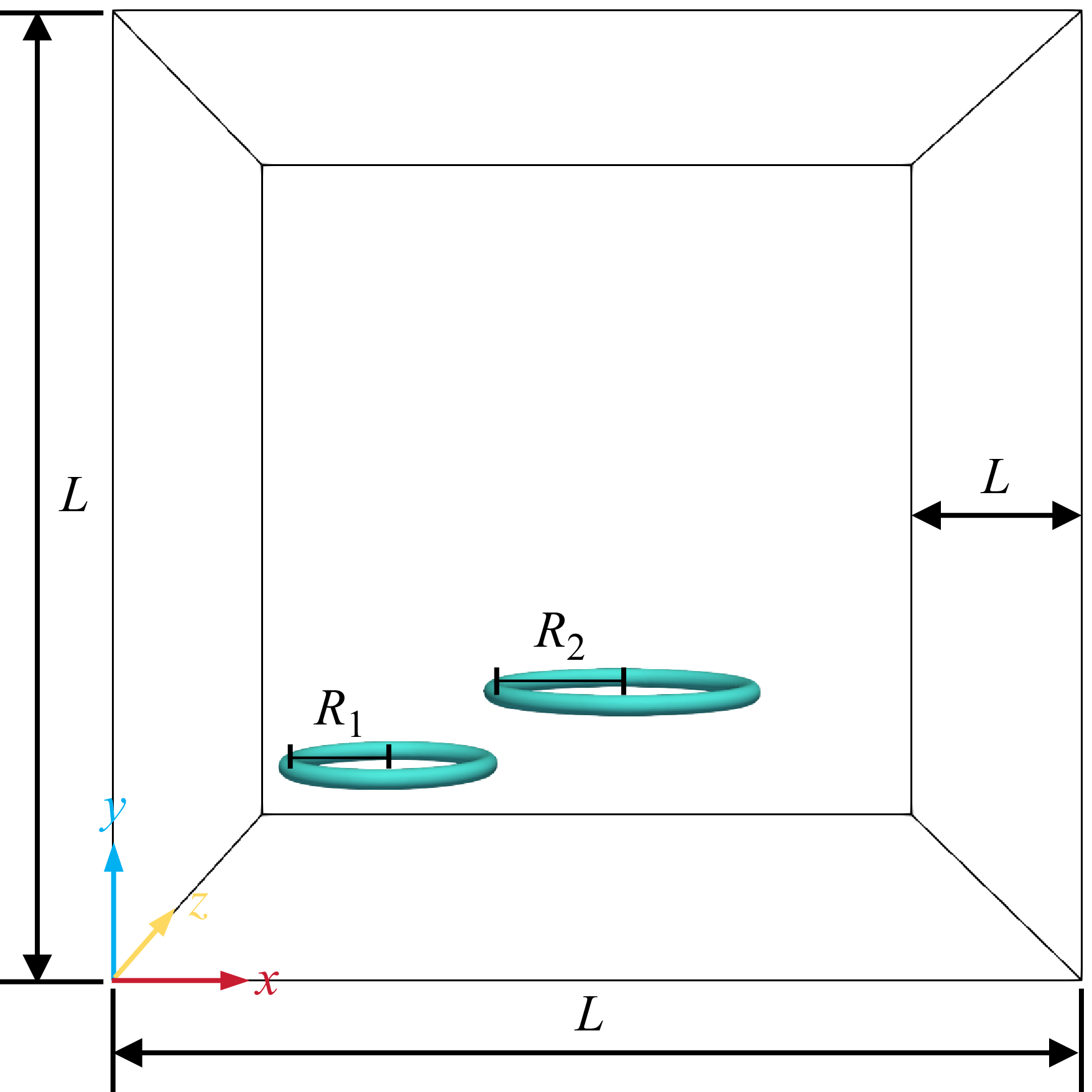
As illustrated in figure 1, the left- and right-hand vortex bubble rings have major radii
 $R_1 = 0.085L$
and
 $R_2 = 0.11L$
, respectively, each approximately one-tenth of the domain size. This keeps the interaction localised, and ensures that the rings stay clear of the domain boundaries during evolution. The difference between
 $R_1$
and
 $R_2$
introduces an asymmetric interaction without altering the basic anti-parallel vortex-ring configuration. The tube radius of each ring is set to
 $r=0.0086L$
to ensure slender toroidal bubbles while maintaining appropriate grid resolution of the tube cross-section. These geometric parameters balance physical representativeness, numerical resolution and computational cost, as larger rings are more affected by domain boundaries during post-reconnection evolution, whereas smaller rings would reduce the number of grid cells across the toroidal interface and vortex core. In this study, all geometric parameters are fixed to isolate the effect of
 $\textit{We}$
.
Schematic of the computational domain and initial configuration for the reconnection of two-phase bubble rings. The domain is a cubic volume of side length
 $L$
. Two toroidal bubbles are initially positioned with major radii
 $R_1 = 0.085L$
and
 $R_2 = 0.11L$
for the left- and right-hand rings, respectively, and with the same tube radius
 $r=0.0086L$
.

The fluid properties represent a typical gas–liquid system, with density and viscosity ratios
 $\rho _l/\rho _g = 1000$
and
 $\mu _l/\mu _g = 100$
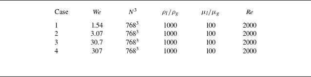
, respectively. As summarised in table 1, the Weber number is varied from
 $1.54$
to
 $307$
to cover the transition from surface-tension-dominated to inertia-dominated interfacial dynamics. The Reynolds number, defined in § 2.4, is fixed at
 $\textit{Re} = 2000$
for all cases.
Parameters for the simulated cases.

Table 1. Long description
A table comparing parameters for simulated cases. The table has four rows and six columns. The columns are labeled Case, We, N cubed, rho l over rho g, mu l over mu g, and Re. The rows are labeled with the following values: Row 1: Case 1, We 1.54, N cubed 768 cubed, rho l over rho g 1000, mu l over mu g 100, Re 2000. Row 2: Case 2, We 3.07, N cubed 768 cubed, rho l over rho g 1000, mu l over mu g 100, Re 2000. Row 3: Case 3, We 30.7, N cubed 768 cubed, rho l over rho g 1000, mu l over mu g 100, Re 2000. Row 4: Case 4, We 307, N cubed 768 cubed, rho l over rho g 1000, mu l over mu g 100, Re 2000.
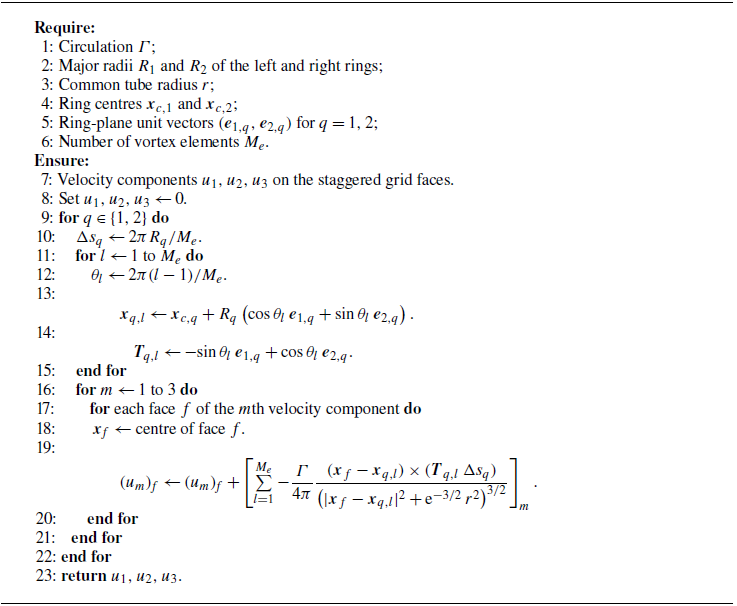
The initial interface of the bubble rings is modelled as a toroidal surface, with the corresponding velocity field generated using the Rosenhead–Moore (RM) vortex filament model (Rosenhead Reference Rosenhead1930; Moore & Saffman Reference Moore and Saffman1972; Saffman Reference Saffman1992)
 \begin{equation} \boldsymbol u(\boldsymbol x, t=0) := \frac {\varGamma }{4\pi } \oint \frac {\boldsymbol \gamma '(s') \times [\boldsymbol x - \boldsymbol \gamma (s')]}{\left [ {\rm e}^{-3/2}\,r^2 + |\boldsymbol x - \boldsymbol \gamma (s')|^2 \right ]^{3/2}} \, \textrm {d}s', \end{equation}
where
 $\varGamma$
denotes the vortex strength,
 $\boldsymbol{\gamma }(s)$
is the parametric equation of the vortex filament, and
 $r$
is the vortex-core regularisation radius, taken to be the same as the initial tube radius of the toroidal bubble. The regularisation term yields a smooth, non-singular initial vorticity field
 $\boldsymbol{\omega } = \boldsymbol{\nabla } \times \boldsymbol{u}$
. As illustrated in figure 1, the two bubble vortex rings are initially positioned with their axes offset in the
 $x$
-direction, forming a non-coaxial arrangement that better reflects the asymmetries encountered in physical realisations. The numerical procedure for the initialisation is detailed in Appendix C.
2.4. Dimensionless parameters
All quantities reported in the following sections are non-dimensionalised using the characteristic scales of the system. The radius of the larger right-hand bubble ring is selected as the characteristic length
 $L_0 = R_2$
, the reference velocity is defined as
 \begin{equation} U_0 = \frac {\varGamma }{2\pi R_2}, \end{equation}
and
 $\varGamma$
is fixed for all cases, so that
 $U_0$
remains constant; the Weber number is varied by adjusting the surface-tension coefficient
 $\sigma$
while keeping the Reynolds number fixed. The characteristic density is chosen as the liquid density,
 $\rho _0 = \rho _l$
.
Based on these characteristic scales, the Reynolds and Weber numbers are defined as
 \begin{equation} \textit{Re} = \frac {\rho _l U_0 L_0}{\mu _l}, \quad \textit{We} = \frac {\rho _l U_0^2 L_0}{\sigma }. \end{equation}
The non-dimensional variables are denoted by a superscript
 $\ast$
. The basic field variables and coordinates are normalised as
 \begin{equation} \boldsymbol{x}^* = \frac {\boldsymbol{x}}{L_0}, \quad \boldsymbol{u}^* = \frac {\boldsymbol{u}}{U_0}, \quad t^* = \frac {t U_0}{L_0}, \quad \kappa ^* = \kappa L_0, \quad \sigma ^* = \frac {\sigma }{\rho _0 U_0^2 L_0} = \frac {1}{\textit{We}}. \end{equation}
The initial offset between the two rings is measured by
 \begin{equation} \chi ^* = \frac {\chi }{L_0}, \end{equation}
where
 $\chi$
denotes the offset between the
 $x$
-projections of the rightmost point of the left-hand ring’s centreline, and the leftmost point of the right-hand ring’s centreline, quantifying the initial relative position.
The computational domain in dimensional coordinates is denoted by
 $V$
, and the corresponding non-dimensional domain is denoted by
 $V^*$
, with
 $\mathrm{d}V^* = \mathrm{d}V / L_0^3$
. The non-dimensional gas volume and bubble centroid are defined as
 \begin{equation} V_g^*(t^*) = \int _{V^*} (1-\alpha )\,\mathrm{d}V^* = \frac {1}{L_0^3}\int _V (1-\alpha )\,\mathrm{d}V \end{equation}
and
 \begin{equation} \boldsymbol{r}_c^*(t^*) = \frac {1}{V_g^*(t^*)} \int _{V^*} \boldsymbol{x}^*(1-\alpha )\,\mathrm{d}V^* . \end{equation}
Here,
 $\boldsymbol{r}_c^*(t^*) = (X^*, Y^*, Z^*)$
denotes the non-dimensional gas-phase centroid, where
 $X^*$
,
 $Y^*$
and
 $Z^*$
are the centroid coordinates in the
 $x$
-,
 $y$
- and
 $z$
-directions, respectively.
The normalised cross-sectional area of the vortex-ring core is defined as
 \begin{equation} A_r^*(t^*) = \frac {A_r(t^*)}{A_{r,0}}, \end{equation}
where
 $A_r$
is the instantaneous cross-sectional area, and
 $A_{r,0}$
is its initial value.
The non-dimensional interfacial area and surface energy are defined as
 \begin{equation} A^*(t^*) = \frac {1}{L_0^2}\int _V |\boldsymbol{\nabla }\alpha |\,\mathrm{d}V, \quad E_\sigma ^*(t^*) = \sigma ^* A^*(t^*). \end{equation}
The total kinetic energy, interfacial kinetic energy, enstrophy and viscous dissipation rate are defined as
 \begin{equation} E_k^*(t^*) = \frac {\displaystyle \int _V \frac {1}{2}\rho\, |\boldsymbol{u}|^2\,\mathrm{d}V} {\rho _0 U_0^2 L_0^3}, \end{equation}
 \begin{equation} E_{ki}^*(t^*) = \frac {\displaystyle \int _V \frac {1}{2}\rho\, |\boldsymbol{u}|^2\, |\boldsymbol{\nabla }\alpha |\,\mathrm{d}V} {\rho _0 U_0^2 L_0^2}, \end{equation}
 \begin{equation} \varOmega ^*(t^*) = \frac {\displaystyle \int _V \frac {1}{2}|\boldsymbol{\omega }|^2\,\mathrm{d}V} {U_0^2 L_0} \end{equation}
and
 \begin{equation} \varepsilon ^*(t^*) = \frac {\displaystyle \int _V 2\mu (\boldsymbol{x})\,\boldsymbol{S}:\boldsymbol{S}\,\mathrm{d}V} {\rho _0 U_0^3 L_0^2}, \end{equation}
where
 $\boldsymbol{S} = [\boldsymbol{\nabla }\boldsymbol{u}+(\boldsymbol{\nabla }\boldsymbol{u})^{\rm T}]/2$
is the strain-rate tensor.
For the helicity analysis, the computational domain is divided into two half-domains by the symmetry plane
 $z = L/2$
:
 \begin{equation} V_+ = \{\boldsymbol{x}\in V \mid z \gt L/2\}, \quad V_- = \{\boldsymbol{x}\in V \mid z \lt L/2\}. \end{equation}
The helicity density and half-domain helicities are non-dimensionalised as
 \begin{equation} h^* = \frac {(\boldsymbol{u}\boldsymbol{\cdot }\boldsymbol{\omega }) L_0}{U_0^2} \end{equation}
and
 \begin{equation} H_+^*(t^*) = \frac {\displaystyle \int _{V_+} \boldsymbol{u}\boldsymbol{\cdot }\boldsymbol{\omega }\,\mathrm{d}V} {U_0^2 L_0^2}, \quad H_-^*(t^*) = \frac {\displaystyle \int _{V_-} \boldsymbol{u}\boldsymbol{\cdot }\boldsymbol{\omega }\,\mathrm{d}V} {U_0^2 L_0^2}. \end{equation}
Finally, the wake retraction velocity used in the pinch-off analysis is defined as
 \begin{equation} u_s^* = \frac {u_s}{U_0}. \end{equation}
Unless otherwise stated, all quantities with superscript
 $\ast$
in the following sections are non-dimensional.
3. Morphological evolution of bubble vortex rings
Spatiotemporal evolution of bubble-ring morphology at different Weber numbers. The gas–liquid interface is shown by the isosurface
 $\alpha =0.5$
. Each column shows a time sequence at
 $t^* = 0, 0.3, 0.6, 0.9, 1.2, 1.5, 1.8$
. Columns correspond to different regimes: (a) inertia-dominated case with
 $\textit{We}=30.7$
, coloured in cyan; (b) transitional case with
 $\textit{We}=3.07$
, coloured in red; (c) surface-tension-dominated case with
 $\textit{We}=1.54$
, coloured in purple.

Figure 2. Long description
Panel A: A sequence of images showing the evolution of a bubble ring in an inertia-dominated case with a Weber number of 30.7. The images are taken at different non-dimensional times (t*) ranging from 0 to 1.8. The bubble ring is colored in cyan. Panel B: A sequence of images showing the evolution of a bubble ring in a transitional case with a Weber number of 3.07. The images are taken at different non-dimensional times (t*) ranging from 0 to 1.8. The bubble ring is colored in red. Panel C: A sequence of images showing the evolution of a bubble ring in a surface-tension-dominated case with a Weber number of 1.54. The images are taken at different non-dimensional times (t*) ranging from 0 to 1.8. The bubble ring is colored in purple.
We investigate the spatiotemporal evolution of bubble vortex rings across different
 $\textit{We}$
using DNS. The gas–liquid interface is identified by the liquid volume fraction isosurface
 $\alpha =0.5$
, as shown in figure 2. The three cases in figure 2 represent a progressive transition from inertia-dominated interfacial stretching to surface-tension-dominated break-up. For the high-
 $\textit{We}$
case
 $\textit{We}=30.7$
, the bubble rings undergo substantial longitudinal stretching, and form elongated interfacial filaments that persist during the simulated evolution. As
 $\textit{We}$
decreases to
 $3.07$
, surface tension increasingly suppresses filament stretching, and localised necking and partial break-up begin to emerge. At the lowest Weber number shown,
 $\textit{We}=1.54$
, the toroidal structure destabilises faster, and fragments into multiple satellite bubbles. The
 $\textit{We}=307$
case is included in the quantitative analyses below but is not shown in this morphology montage because its interface evolution is qualitatively similar to the
 $\textit{We}=30.7$
case over the present time interval. Overall, the interaction of the anti-parallel pair progresses through four characteristic phases: kinematic approach, interfacial reconnection, helicity transport and capillary pinch-off.
3.1. Phase I: initial approach
At
 $t^*=0$
, two bubble vortex rings are arranged anti-parallel, consistent with the high-Reynolds-number configurations of van Rees et al. (Reference van Rees, Hussain and Koumoutsakos2012) and Shen et al. (Reference Shen, Ostilla-Mónico and Zhu2025). The mutual induction between the rings superimposes an additional translational velocity onto their self-induced motion, driving them towards the collision zone.
In the reference configuration with
 $\chi ^*=0$
, the
 $x$
-projection of the rightmost point of the left-hand ring centreline coincides with that of the leftmost point of the right-hand ring centreline. Different offset cases are generated by keeping the left-hand ring fixed and translating only the right-hand ring along the
 $x$
-direction. A positive
 $\chi ^*$
corresponds to translating the right-hand ring in the positive
 $x$
-direction, and a negative
 $\chi ^*$
corresponds to translating it in the negative
 $x$
-direction.
Figure 3 illustrates the definition of the initial
 $x$
-direction offset and the corresponding early-stage interfacial deformation. As the rings approach, the intensified strain-rate field induces stretching and bending of the inner interface. The initial offset controls the relative alignment of the two approaching ring segments, thereby modifying the local deformation near the collision zone. For a small dimensionless offset, e.g.
 $\chi ^*=\pm 0.15$
, the approaching segments remain closely aligned, leading to pronounced local warping and distortion. In contrast, a larger initial offset produces a more asymmetric approach configuration and a smoother interfacial profile near the interaction region. This initial difference in local curvature and interface morphology subsequently affects the location and morphology of the reconnection points. The visualisations in figure 3 confirm that the initial offset modifies the local warping and deformation of the approaching inner interface before reconnection.
Definition of the initial spatial offset and early-stage interfacial deformation of the bubble rings. (a) Schematic illustration of the
 $x$
-direction offset
 $\chi ^*$
. (b) Representative interface morphologies at the initial time
 $t^*=0$
and at the later approach time for different dimensionless offsets.

3.2. Phase II: interfacial reconnection process
Reconnection involves a topological change in the flow as two previously distinct fluid domains merge. The process begins with the drainage and rupture of the intervening liquid film, leading to the formation of a connecting bridge between the bubble rings.
Figure 4(a) shows the evolution of the central reconnection region, where the bridge dynamics is governed by the competition between inertial stretching and capillary retraction. At
 $\textit{We} = 307$
, represented by the pink isosurface, inertial forces dominate the dynamics, stretching the interface into a slender bridge that persists for an extended period, with surface tension remaining too weak to drive rapid contraction. In contrast, for
 $\textit{We} = 3.07$
, represented by the light blue isosurface, surface tension governs the evolution. The high curvature at the neck is associated with enhanced capillary retraction and faster drainage of the intervening liquid film, leading to a more rapid collapse of the bridge. The cross-sectional views in figure 4(b) further confirm that the reconnecting bridge remains elongated for a longer time at high
 $\textit{We}$
, whereas at low
 $\textit{We}$
, surface tension rapidly contracts the interfacial neck and accelerates bridge collapse.
Comparison of interface morphologies and vorticity evolution in the core reconnection region for two Weber numbers. (a) Superposed interface isosurfaces (
 $\alpha = 0.5$
) for
 $\textit{We} = 307$
, denoted in pink, and
 $\textit{We} = 3.07$
, denoted in light blue. (b) Temporal evolution of the cross-section on the symmetry plane
 $z = L/2$
, coloured by vorticity magnitude
 $|\boldsymbol{\omega }|$
.

To distinguish the interfacial topology from the vortical topology, figure 5 compares the phase-fraction interface and the vorticity-magnitude contour for
 $\textit{We}=3.07$
. During the approach and reconnection stages, the
 $|\boldsymbol{\omega }|=2$
contour remains close to the
 $\alpha =0.5$
interface, indicating a close correspondence between the motion of the toroidal bubble and the associated vorticity distribution. At the late pinch-off stage, the gas–liquid interface undergoes a faster topological change, while the vorticity field retains residual structures near the symmetry region. Thus the pinch-off observed from the phase-fraction field is interpreted primarily as an interfacial topological change, rather than as direct evidence of an instantaneous separation of a vortex ring.
Comparison between the bubble-ring interface and the vortex structure at
 $\textit{We}=3.07$
. The orange contours denote the phase-fraction interface
 $\alpha = 0.5$
, and the purple contours denote the vorticity contour
 $|\omega | = 2$
at various times.

Locally magnified views of vortex structures in the reconnection region for two representative Weber numbers at approximately
 $t^* = 0.6$
. The semi-transparent white surfaces are isosurfaces of vorticity magnitude
 $|\boldsymbol{\omega }|=3.5$
, used to visualise the vortex-core regions. The red, green and black curves denote selected vortex lines. The middle images isolate these vortex lines to highlight the coherence and spatial organisation of the vortex-line bundle, and the right-hand images show the vorticity magnitude distribution on the cross-section.

Figure 6. Long description
Panel A: A 3D visualization showing vortex structures in the reconnection region for a Weber number of 307. The semi-transparent white surfaces represent isosurfaces of vorticity magnitude, highlighting the vortex-core regions. The red, green, and black curves denote selected vortex lines. The middle image isolates these vortex lines to emphasize the coherence and spatial organization of the vortex-line bundle. The right-hand image displays the vorticity magnitude distribution on the cross-section, with a color scale ranging from 0 to 5. Panel B: A 3D visualization showing vortex structures in the reconnection region for a Weber number of 1.54. The semi-transparent white surfaces represent isosurfaces of vorticity magnitude, highlighting the vortex-core regions. The red, green, and black curves denote selected vortex lines. The middle image isolates these vortex lines to emphasize the coherence and spatial organization of the vortex-line bundle. The right-hand image displays the vorticity magnitude distribution on the cross-section, with a color scale ranging from 0 to 5.
Figure 6 presents locally magnified views of the vortex structures for two representative Weber numbers, where the vortex cores are identified by the vorticity-magnitude isosurface
 $|\boldsymbol{\omega }| = 3.5$
, while the red, green and black lines visualise the spatial organisation and coherence of the vortex bundle. For the high-
 $\textit{We}$
case in figure 6(a), inertial effects dominate vortex stretching and transport, while the relative influence of surface tension on the vortex structure is weak. The vortex-line bundle remains compact and coherent. Vortex lines seeded from the same local region are approximately aligned with the local vortex-core centreline, and show only weak lateral deformation, with no evident large-amplitude coiling or branching. For the low-
 $\textit{We}$
case in figure 6(b), the vortex-line bundle becomes less coherent. The selected vortex lines wind around the local bundle path with a visibly larger coiling radius, forming loose and large-amplitude coils. In addition, multi-level branching structures develop in the leg region, curving and extending around the main vortex structure, and broadening the reconnection region along the circumferential direction of the vortex ring.
The two-dimensional vorticity insets on the right-hand side of figure 6 further support the correlation between vortex-line organisation and vorticity distribution. Under the low-
 $\textit{We}$
condition, vorticity concentrates in the high-curvature regions associated with large-amplitude coiling and bifurcating branches, forming localised vorticity clusters with pronounced intensity peaks. Under the high-
 $\textit{We}$
condition, the vorticity distribution remains smooth and diffuse, consistent with the compact and coherent vortex structure, as dominant inertial effects preserve coherent vorticity transport, while the relatively weak influence of surface tension suppresses pronounced local distortion or vorticity segregation.
3.3. Phase III: transport of helicity
When originally anti-parallel vortex lines reconnect into an interconnected topological structure, the system dynamics shifts from topological discontinuity to wave propagation, accompanied by strong local twisting and redistribution of vorticity.
As shown in figure 7, the twisting disturbance generated at the reconnection point propagates along the vortex structure towards the undisturbed ends of the vortex rings in the form of Kelvin waves. The propagation velocity, wavelength and morphology of these waves are modulated by surface tension. Under low-
 $\textit{We}$
conditions in figures 7(c,d), the higher surface tension provides a stronger capillary restoring force, supporting Kelvin waves with higher group velocities. Consequently, helical perturbations reach the ends of the vortex rings earlier, causing the entire vortex rings to enter an oscillatory relaxation state more rapidly. Under high-
 $\textit{We}$
conditions shown in figures 7(a,b), the ‘winding’ morphology directly reflects the reconnection-induced torsional effect. This torsional effect redistributes the concentrated energy and angular momentum accumulated in the contact zone during collision throughout the entire vortex-ring structure, thereby establishing the flow-field foundation for the subsequent pinch-off process.
Schematic of the half-sectioned interface along the positive
 $z$
domain illustrating helicity transport. (a,b) For
 $\textit{We} = 30.7$
, coloured in cyan, where (b) is a magnified view of the yellow dashed box in (a). (c,d) For
 $\textit{We} = 3.07$
, coloured in red, where (d) is a magnified view of the purple dashed box in (c).

Schematic of the shedding and pinch-off mechanisms. (a) Comparison of wake morphologies at high and low Weber numbers. The wake encircled by the black box shows a magnified view on the
 $x$
–
 $z$
plane of the overall wake morphology on the
 $x$
–
 $y$
plane. The cyan translucent region represents the wake at
 $\textit{We} = 30.7$
, whereas the red interface corresponds to the wake at
 $\textit{We} = 3.07$
, highlighting that an increasing Weber number suppresses pinch-off and promotes elongated, persistent wake connectivity. (b–e) Wake evolution for different Weber numbers. At low
 $\textit{We}$
, denoted by the pink line, the evolution proceeds from an inertial-dominated phase in (b–d), marked by vortex filament elongation and secondary ring shedding, to a capillary-dominated regime in (e), where rapid surface-tension-driven retraction produces clean pinch-off via the Rayleigh–Plateau instability. In contrast, at high
 $\textit{We}$
, represented by the blue and cyan filaments, weaker surface-tension effects delay the shedding process.

Geometric evolution and motion statistics of bubbles at different
 $\textit{We}$
values, including only bubbles with volumes exceeding
 $1\,\%$
of the initial vortex-ring volume. (a) Temporal evolution of discrete bubble number
 $N_g$
. (b) Bubble centroid trajectories
 $r^*_c(X^*,Y^*)$
.

3.4. Phase IV: pinch-off and break-up
The final phase of evolution involves the break-up of the connecting filament and the shedding of substructures. This process is very sensitive to the Weber number, and follows the classic Rayleigh–Plateau instability mechanism in vortex-dominated multi-phase flows.
Figure 8(a) compares representative wake morphologies for high and low Weber numbers, and figure 8(b–e) schematically illustrate the corresponding shedding and pinch-off mechanisms.
For high-
 $\textit{We}$
conditions, inertial stretching dominates over capillary retraction. As shown by the blue and cyan trajectories in figures 8(b–e), the connecting filament stays elongated for a longer time, and necking is delayed because the surface tension is insufficient to rapidly contract the stretched bridge. This delayed break-up leads to a more persistent wake connection and a more disordered shedding morphology, with satellite fragments and residual filamentary structures, as illustrated in figure 8(a).
For low-
 $\textit{We}$
conditions, capillary-driven necking is more effective. As shown by the pink trajectory in figures 8(b–e), the connecting filament retracts more rapidly after the initial elongation stage, and eventually undergoes clean pinch-off. This process severs the connecting tail, and produces a more compact secondary structure with fewer residual fragments.
4. Geometric characteristics and topological statistics
4.1. Topological evolution of discrete bubbles
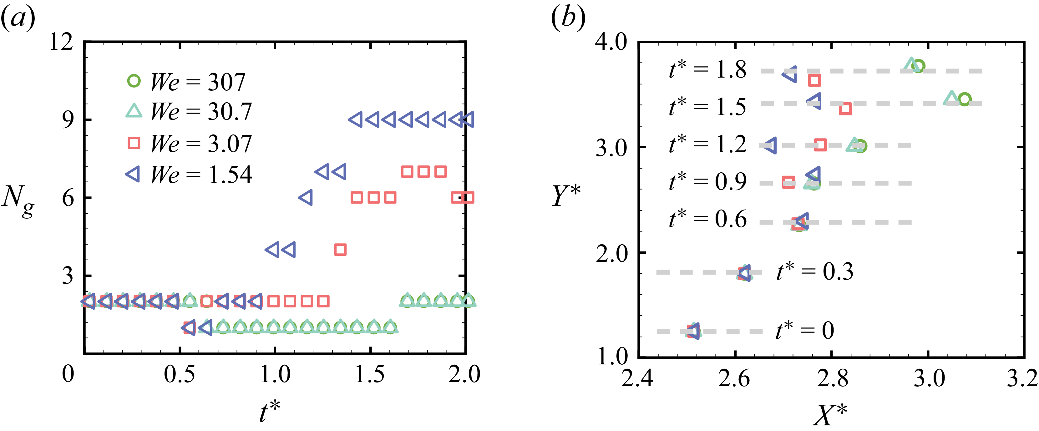
The number of discrete gas bubbles,
 $N_g$
, is introduced to quantify the connectivity of gas–liquid interfaces and the associated topological complexity in the multi-phase flow. Figure 9(a) shows the temporal evolution of
 $N_g$
, where only bubbles with volumes larger than 1 % of the initial bubble-ring volume are included in the counting. Its evolution corresponds to the four-stage morphological dynamics qualitatively described in § 3.
During the initial approach phase with
 $t^* \lt 0.5$
, corresponding to phase I,
 $N_g$
remains at its initial value 2, indicating that bubble-ring interactions are limited to velocity-induced geometrical deformation. The accumulated energy is insufficient to induce interfacial topological transitions or to form medium-to-large bubbles above the statistical threshold. Upon entering the interfacial reconnection phase at
 $t^* \approx 0.6$
, corresponding to phase II,
 $N_g$
abruptly drops to 1, a discrete jump that marks a topological singularity in the flow field. This signifies that the two initially separate bubble rings have overcome the repulsive resistance of the intervening liquid film and merged into a single connected domain. Notably, low-
 $\textit{We}$
cases with
 $\textit{We} = 1.54$
and
 $3.07$
exhibit minor oscillations in
 $N_g$
during the reconnection transition phase. In the subsequent pinch-off and break-up phase for
 $t^* \gt 1.2$
, corresponding to phase IV, the evolution of
 $N_g$
diverges markedly across Weber numbers, directly reflecting differences in the post-reconnection generation and evolution of medium-to-large bubbles.
The analysis reveals a bifurcated influence of the Weber number on the evolution of
 $N_g$
. At low
 $\textit{We}$
, strong surface tension rapidly triggers Rayleigh–Plateau instability (Eggers & Villermaux Reference Eggers and Villermaux2008), breaking stretched ligaments into medium-sized bubbles above the statistical threshold, which leads to significant growth and elevated
 $N_g$
. During the reconnection transition, alternating dominance of surface tension and inertia produces weak oscillations in
 $N_g$
without inducing topological splitting, resembling the capillary- and centrifugal-acceleration-induced interface cycles observed by Lo et al. (Reference Lo, Liu, Alghamdi, Afzaal and Thoroddsen2025). At high
 $\textit{We}$
, the dominance of fluid inertia leads mainly to sub-threshold satellite bubble formation, and suppresses contact–separation cycles, resulting in
 $N_g$
remaining nearly constant with minimal variation. This contrast confirms that strong surface tension at low
 $\textit{We}$
both promotes medium-sized bubble formation and induces interface oscillations, whereas inertia at high
 $\textit{We}$
prevents significant bubble generation and cyclic dynamics, yielding a statistically distinct
 $N_g$
signature.
Figure 9(b) plots the projected gas-phase centroid trajectories on the
 $X^*$
–
 $Y^*$
plane. Trajectory analysis reveals consistent vertical displacement components
 $Y^*$
across all cases, indicating that the upward translational motion is only weakly affected by variations in
 $\textit{We}$
. In contrast, the radial expansion component
 $X^*$
normalised by
 $L_0$
is strongly regulated by surface tension. High-
 $\textit{We}$
cases undergo larger radial expansion and continue propagating outwards over time, whereas low-
 $\textit{We}$
cases display suppressed lateral spreading and even slight contraction at later stages. This behaviour suggests that at low
 $\textit{We}$
, stronger surface-tension effects generate centripetal restoring forces that resist vorticity-induced radial expansion and promote a more compact vortex-ring structure.
4.2. Cross-sectional redistribution during reconnection
Temporal evolution of dimensionless
 $z$
semi-axis cross-sectional area
 $A_r^*$
for two bubble rings at Weber numbers
 $\textit{We} = 3.07$
,
 $30.7$
and
 $307$
. Positions A and D denote the bubble ring ends farthest from the reconnection zone, while positions B and C indicate the reconnection contact regions.

Figure 10 reveals fine-scale gas-phase redistribution during reconnection by tracking dimensionless cross-sectional area evolution at different bubble-ring positions. Positions A and D, representing the bubble ring ends farthest from the reconnection regions, exhibit an anti-correlated response relative to positions B and C, driven by gas-phase compression and redistribution during collision. During the initial approach phase at
 $t^* \lt 0.5$
, all positions show minor fluctuations around initial values, indicating predominant whole-ring translation and mild stretching without significant radial volume redistribution. As evolution enters the interfacial reconnection phase from
 $t^* \approx 0.5$
to
 $t^* \approx 0.8$
, positions B and C experience strong compression from vortex collisions, causing continuous cross-sectional area reduction and flattening. This compression forces gas-phase migration towards ends A and D, synchronously increasing their cross-sectional areas.
The redistribution is strongly regulated by the Weber number. At low
 $\textit{We} = 3.07$
, the cross-sectional areas of positions B and C decrease more sharply and rapidly, while the areas of positions A and D increase correspondingly. Strong surface tension accelerates compression at the reconnection regions, and drives gas-phase migration, followed by rapid post-reconnection reflux at ends A and D that preserves bubble-ring integrity. In contrast, at high
 $\textit{We} = 307$
, inertial forces weaken the compression effect. Area reductions at positions B and C are more gradual, with minima remaining higher, while the growth magnitude and rate at positions A and D are reduced. No significant reflux occurs in the late stages, reflecting lower gas migration efficiency under inertial dominance. These observations confirm that surface tension at low Weber number enhances the efficiency of reconnection-induced redistribution, promoting rapid geometric adjustment and stabilisation of the bubble ring.
4.3. Surface energy and curvature dynamics
The interfacial area
 $A^*$
, surface energy
 $E_\sigma ^*$
, and mean curvature
 $\kappa ^*$
are used to characterise the geometric and energetic response of the gas–liquid interface during reconnection and pinch-off. These quantities are evaluated according to the definitions given in § 2.4. Figure 11 presents their temporal evolution for different Weber numbers.
As shown in figure 11(a), the curve
 $A^*(t^*)$
exhibits two distinct drops, associated respectively with the interfacial reconnection phase and the subsequent pinch-off process. At
 $t^* \approx 0.6$
, corresponding to the reconnection moment, the first decrease occurs as redundant interfaces vanish during bubble-ring fusion, releasing surface energy, with low-
 $\textit{We}$
cases decreasing earlier due to faster capillary wave propagation that accelerates topological adjustment towards minimum-area configurations. During the pinch-off stage at
 $t^* \approx 1.5$
, different Weber numbers produce dramatic divergence. Low
 $\textit{We} = 1.54$
exhibits a steep
 $A^*$
reduction, reflecting intense capillary retraction. Strong surface tension overcomes viscous resistance, driving liquid bridge contraction and break-up to form compact spherical structures with minimal surface energy. In contrast, high
 $\textit{We} = 307$
shows a gradual reduction over longer durations with smaller magnitudes, as inertial dominance sustains interface stretching, resists capillary contraction, and prolongs the existence of elongated ligament structures, delaying surface energy dissipation and minimisation.
Evolution of surface energy and curvature for bubble interfaces at different Weber numbers over time. (a) Normalised surface area
 $A^*$
as a surface energy proxy. (b) Normalised mean curvature
 $\kappa ^*$
.

Curvature divergence corresponds to singular neck formation, where the local radius
 $R \to 0$
would cause the capillary velocity
 $v_\sigma \sim \sqrt {\sigma /\rho R}$
to diverge in the inviscid limit. This extreme capillary velocity dominates local flow, accelerating neck contraction, and leading to rapid bubble detachment accompanied by a pronounced decrease in surface area. Figure 11(b) shows the evolution of the normalised mean curvature
 $\kappa ^*$
, indicating microscopic geometric changes in surface area. Low-
 $\textit{We}$
cases exhibit reduced curvature during the late stages, indicating stronger capillary-driven interface relaxation and contraction, whereas high-
 $\textit{We}$
cases develop pronounced late-time growth in
 $\kappa ^*$
associated with inertia-driven neck stretching prior to pinch-off.
5. Energetics and vorticity dynamics
Energy evolution and dissipation characteristics at different
 $\textit{We}$
. (a) Total kinetic energy
 $E_k^*$
. (b) Interfacial kinetic energy
 $E_{ki}^*$
. (c) Total enstrophy
 $\varOmega ^*$
. (d) Viscous dissipation rate
 $\varepsilon ^*$
.

5.1. Energy cascade and capillary-enhanced dissipation
The total kinetic energy
 $E_k^*$
characterises the global kinetic energy of the two-phase flow, whereas the interfacial kinetic energy
 $E_{ki}^*$
measures the kinetic energy localised near the gas–liquid interface through the weighting factor
 $|\boldsymbol{\nabla }\alpha |$
.
Figure 12(a) presents the temporal decay of the total kinetic energy. Low-
 $\textit{We}$
cases exhibit more rapid energy decay and larger enstrophy and dissipation peaks than high-
 $\textit{We}$
cases. Given that the Reynolds number is fixed, the variation in energy decay is closely associated with capillary effects. Strong surface tension provides a high-frequency restoring force, causing the deformed interface to rebound rapidly, and exciting a series of capillary waves, thereby promoting the transfer of kinetic energy from large-scale advective motion towards smaller interfacial scales. This transfer constitutes a capillary-enhanced energy cascade. Figure 12(b) shows that
 $E_{ki}^*$
decreases rapidly during the early stage of evolution, indicating a continuous reduction of interface-localised kinetic energy as the bubble rings expand and decelerate. After reconnection, the decay rate slows down and the curves gradually separate for different
 $\textit{We}$
. The higher-
 $\textit{We}$
cases retain slightly larger values of
 $E_{ki}^*$
at late times, suggesting more persistent interfacial motion due to weaker capillary restoring effects, whereas lower-
 $\textit{We}$
flows exhibit faster attenuation of interface-region kinetic energy under stronger surface-tension-induced smoothing.
Since the viscous dissipation rate is proportional to the square of the velocity gradient, the accumulation of energy at small scales greatly enhances dissipation efficiency. The viscous dissipation rate
 $\varepsilon ^*$
, defined in § 2.4, quantifies the conversion of kinetic energy into heat through velocity gradients. As shown in figure 12(d), the dependence of
 $\varepsilon ^*$
on
 $\textit{We}$
is stage-dependent. During the reconnection stage at
 $t^* \approx 0.6$
, the intermediate- and high-
 $\textit{We}$
cases exhibit more pronounced dissipation peaks, indicating stronger local velocity-gradient enhancement during the main reconnection event. During the later pinch-off stage at
 $t^* \approx 1.4$
–
 $1.5$
, the lower-
 $\textit{We}$
cases instead show secondary dissipation peaks, corresponding to capillary-driven neck contraction and rapid break-up of the connecting filament. Thus decreasing
 $\textit{We}$
does not uniformly increase the dissipation rate throughout the evolution; rather, it shifts the main dissipation enhancement from the reconnection stage to the subsequent capillary pinch-off stage.
The enstrophy
 $\varOmega ^*$
, defined in § 2.4, measures the global intensity of the vorticity field. As shown in figure 12(c), the enstrophy
 $\varOmega ^*$
exhibits a sharp peak during the reconnection event at
 $t^* \approx 0.6$
, indicating a rapid strengthening and redistribution of vorticity in the reconnection region. This enhancement is associated with the strong interfacial deformation and curvature variation during reconnection, and may reflect the combined effects of interfacial vorticity generation, vorticity advection and vortex stretching (Saffman Reference Saffman1990; Terrington et al. Reference Terrington, Hourigan and Thompson2022).
5.2. Helicity transport and half-domain topological characteristics
In the current colliding bubble-ring system, the initial flow field exhibits mirror symmetry about the plane
 $z = L/2$
. The pseudo-scalar nature of helicity implies that mirror reflection reverses its sign, with the helicity on the two sides of the symmetry plane being approximately equal in magnitude and opposite in sign at any instant. This results in the global net helicity
 $H(t) \approx 0$
being always satisfied (Moffatt Reference Moffatt1969; Wang et al. Reference Wang, Pang, Li, Yan, Kang, Zhang and Xiong2026). However, the zero integral value masks the underlying topological dynamics, where local fluid elements undergo strong torsion and entanglement that are offset by global symmetry.
Mathematical and numerical analyses have demonstrated that for anti-parallel reconnection configurations, the writhe of the centrelines is conserved (Laing et al. Reference Laing, Ricca and Sumners2015). Consequently, the self-helicity of the interacting vortex rings can remain invariant throughout the purely anti-parallel reconnection process, provided that the intrinsic twist is preserved without anomalous injection at the reconnection site (Laing et al. Reference Laing, Ricca and Sumners2015; Zuccher & Ricca Reference Zuccher and Ricca2015). To reveal the hidden evolution of the topological structure, we divide the computational domain into two mirror-related subdomains, denoted by
 $V_+$
and
 $V_-$
, on the two sides of the symmetry plane
 $z = L/2$
, and introduce the non-dimensional half-domain helicities
 $H_+^*$
and
 $H_-^*$
, as defined in § 2.4.
Figure 13(a) shows regions of high helicity density originating from the neck region where reconnection occurs, and propagating along the vortex core, closely matching the spatial distribution of Kelvin waves observed through three-dimensional reconstruction by Minowa et al. (Reference Minowa, Yasui, Nakagawa, Inui, Tsubota and Ashida2025). Figure 13(b) shows the temporal evolution of the half-domain helicity for different Weber numbers. As the system approaches the reconnection critical point at
 $t^* \approx 0.6$
, a topological transition occurs. The helicities in the two mirror-related half-domains,
 $H_+^*$
and
 $H_-^*$
, rapidly diverge in magnitude while maintaining an anti-symmetric distribution, with
 $H_+^* \approx -H_-^*$
. This divergence reflects the breaking of the initial mirror symmetry in the helicity distribution at the reconnection point.
This reconnection event instantaneously introduces a strong torsional component at the reconnection site, namely the ‘elbow’ region, transforming the initially simple ring topology into a locally knotted structure. This is consistent with experimental observations by Stasiak et al. (Reference Stasiak, Xing, Alihosseini, Barenghi, Baggaley, Guo, Galantucci and Krstulovic2025) in superfluid helium, where vortex reconnection acts as a topological singularity that generates complexity through vortex-line breaking and rejoining, accompanied by the excitation of Kelvin waves that transport helicity away from the reconnection site along the vortex core.
Propagation of helicity and anti-symmetric half-domain dynamics. (a) Instantaneous flow visualisation using an isosurface of vorticity magnitude coloured by the local helicity density, illustrating the spatiotemporal pathway of torsional waves triggered by reconnection and propagating outwards along the vortex rings. (b) Evolution of the total helicity in the
 $V_-$
half-domain,
 $H_-^*$
.

Figure 13. Long description
Panel A: This panel shows a series of three-dimensional visualizations of fluid flow at different time points (t* = 0.3, t* = 0.6, t* = 0.9). The visualizations use isosurfaces of vorticity magnitude colored by local helicity density to illustrate the spatiotemporal pathway of torsional waves. The color scale on the left indicates the magnitude of helicity density, ranging from 0 to 50. The visualizations depict the propagation of spiral waves along vortex rings. Panel B: This panel presents a line graph showing the evolution of the total helicity in the half-domain (H*) over time (t*). The x-axis represents the dimensionless time (t*), ranging from 0.6 to 1.4. The y-axis represents the total helicity (H*), ranging from -60 to 180. The graph includes four different lines, each representing a different Weber number (We = 307, We = 30.7, We = 3.07, We = 1.54). The lines show how the total helicity evolves over time for each Weber number, with distinct trends and patterns visible for each case.
The Weber number regulates the stability of topological evolution. For high-
 $\textit{We}$
cases with
 $\textit{We} = 30.7$
and
 $307$
, represented by the green and cyan curves, the system exhibits large-amplitude alternating oscillations. Inertia dominates in this regime, and weak surface tension provides insufficient restoring force to constrain the pronounced geometric deformation of the vortex rings after reconnection. Consequently, the vortex cores undergo significant distortion, stretching and rebound, leading to repeated sign reversals of the half-domain helicity
 $H_{\pm }^{*}$
. The large jumps of the helicity curves between positive and negative values indicate a topologically unsteady state with weak capillary constraint, where violent vortex filament writhing dominates late-stage evolution. For the low-
 $\textit{We}$
case with
 $\textit{We} = 1.54$
, represented by the purple curve, helicity oscillations are strongly suppressed, with only small fluctuations present. In this regime, surface tension minimises the interfacial area and constrains large-scale torsional deformation of the vortex structure. The resulting rapid stabilisation of topological complexity supports small-amplitude Kelvin wave propagation, suppressing inertial topological pulsations, and improving stability.
5.3. Exploration of the critical Weber number in the pinch-off stage
Schematic of the velocity statistical method and wake retraction velocity evolution during the pinch-off stage under different Weber numbers. (a) Representative snapshot at approximately
 $t^* = 1.5$
showing the selection of the wake-tip reference points used to evaluate the wake retraction velocity. (b) Temporal evolution of the wake retraction velocity
 $u_s^*$
under different
 $\textit{We}$
during the pinch-off stage. The dashed vertical line marks
 $t^* = 1.54$
, where the ordering of
 $u_s^*$
among different
 $\textit{We}$
begins to change.

Figure 14. Long description
Panel A: A schematic diagram shows a snapshot of the wake-tip reference points used to evaluate the wake retraction velocity. The diagram includes arrows pointing to different locations along the wake, each labeled with a specific Weber number (We) value. The values range from We = 3.07 to We = 30.7, indicating different conditions under which the measurements were taken. Panel B: A scatter plot illustrates the temporal evolution of the wake retraction velocity under different Weber numbers during the pinch-off stage. The x-axis represents the dimensionless time (t*) ranging from 1.4 to 1.6, and the y-axis represents the dimensionless wake retraction velocity (u_s*) ranging from 0 to 16. Different symbols and colors represent different Weber numbers: triangles for We = 30.7 and We = 12.3, circles for We = 7.68 and We = 6.14, and squares for We = 4.09 and We = 3.07. A dashed vertical line at t* = 1.5 marks the point where the ordering of wake retraction velocities among different Weber numbers begins to change.
To explore the critical Weber number governing the dynamics of the bubble ring during the pinch-off stage, we further subdivide the intermediate Weber number cases between
 $\textit{We} = 3.07$
and
 $\textit{We} = 30.7$
. The wake retraction velocity
 $u_s^*$
, defined in § 2.4, quantifies the capillary-driven retraction of the secondary structure after the onset of pinch-off.
Figure 14(a) presents a representative snapshot at approximately
 $t^* = 1.5$
, illustrating the wake-tip reference points used to evaluate the wake retraction velocity under different Weber numbers, where the reference point is defined as the tip of the wake structure attached to the main vortex ring. As the Weber number increases, the wake structure becomes progressively elongated, indicating that increasing inertial effects suppress capillary-driven necking and delay the liquid-bridge rupture process.
Figure 14(b) shows the temporal evolution of the wake retraction velocity
 $u_s^*$
during the capillary pinch-off stage. At
 $t^* = 1.4$
, for cases with
 $\textit{We} \gt 12.3$
,
 $u_s^*$
is nearly zero, indicating that these inertia-dominated cases have not yet initiated substantial capillary pinch-off. For
 $\textit{We} \lt 12.3$
,
 $u_s^*$
increases monotonically as
 $\textit{We}$
decreases, reflecting enhanced surface-tension-driven pinch-off and faster growth of the Rayleigh–Plateau instability.
The dashed vertical line at
 $t^* = 1.54$
marks a transition in the relative wake-retraction response. Before this time, lower-
 $\textit{We}$
cases generally have larger
 $u_s^*$
because stronger surface tension drives earlier capillary pinch-off. After this time, the low-
 $\textit{We}$
cases have mostly completed the rapid retraction process, while delayed retraction becomes more pronounced in several higher-
 $\textit{We}$
cases, particularly
 $\textit{We}=12.3$
. Thus the early-time monotonic ordering of
 $u_s^*$
with respect to
 $\textit{We}$
is no longer maintained, although the
 $\textit{We}=30.7$
case does not exhibit a strict reversal, and its retraction remains comparatively weak.
6. Conclusions
This work investigates the topological reconnection of two vortex bubble rings in two-phase flow, focusing on how the Weber number governs the competition between surface tension and inertia at fixed Reynolds number. The reconnection dynamics follows four stages, namely kinematic approach, interfacial reconnection, helicity-wave transport and capillary pinch-off. Low
 $\textit{We}$
promotes clean capillary break-up into daughter bubbles via the Rayleigh–Plateau instability, whereas high
 $\textit{We}$
produces fragmented ligaments and secondary vortical structures.
The approach phase is dominated by the mutual induction of anti-parallel vortex rings, with the initial spatial offset governing the pre-reconnection interfacial deformation. Reconnection onset is marked by significant vorticity flux rearrangement towards the contact region, and instantaneous release of surface energy. Decreasing
 $\textit{We}$
advances this onset and produces a larger reduction of interfacial area. In the reconnection phase, strong surface tension promotes liquid-bridge contraction through capillary retraction, suppressing small-scale interfacial wrinkling.
For helicity transport, surface tension suppresses large-amplitude helicity oscillations. Under low-
 $\textit{We}$
conditions, it stabilises Kelvin wave propagation, while high-
 $\textit{We}$
cases exhibit violent anti-symmetric helicity pulsations. In the pinch-off stage, the wake retraction velocity reveals critical Weber number approximately 12.3, separating capillary-driven pinch-off at low Weber numbers from inertia-dominated stretching and delayed break-up at high Weber numbers.
In future work, we may expand the parameter space to include the Reynolds number and gas–liquid density ratio, as well as incorporating realistic boundary conditions such as gravity and wall confinement. Advanced experimental diagnostics would also allow direct validation of the present results.
Funding
The authors acknowledge the support of the National Natural Science Foundation of China (grant nos 12302294, 12432010 and 12402308).
Declaration of interests
The authors report no conflict of interest.
Appendix A. Grid-convergence assessment and boundary-vorticity diagnostic
We perform a two-phase grid-convergence test using the same gas–liquid property ratios as in the main simulations. The test is conducted for
 $\textit{We} = 3.07$
, where surface-tension effects are relatively strong, and the interface undergoes pronounced deformation. All other parameters are kept consistent with the configuration described in § 2.3.
Grid-convergence assessment for the two-phase bubble-ring reconnection case at
 $\textit{We}=3.07$
, with density and viscosity ratios
 $\rho _l/\rho _g=1000$
and
 $\mu _l/\mu _g=100$
. The curves show the temporal evolution of the normalised kinetic energy
 $E_k/E_{k,0}$
at three resolutions,
 $N=256$
,
 $512$
and
 $768$
. Grey vertical lines mark representative times where interface shapes are shown. The interface is represented by the
 $\alpha =0.5$
isosurface. Green, yellow and blue snapshots correspond to
 $N=256$
,
 $512$
and
 $768$
, respectively.

Vorticity profiles
 $|\boldsymbol{\omega }|$
along
 $x$
on the mid-plane
 $z=0.5L$
at selected
 $(y/L, t^*)$
pairs:
 $(0.01,0.0)$
,
 $(0.21,0.6)$
,
 $(0.31,1.2)$
and
 $(0.39,1.8)$
.

Figure 16. Long description
The image contains four line graphs showing vorticity profiles along the mid-plane at selected time points. Each graph represents a different non-dimensional time value, t*, with corresponding y/L values. Panel A: The line graph for t* = 01 shows the vorticity magnitude |ω| on the vertical axis and the normalized position x/L on the horizontal axis. The graph indicates multiple peaks in vorticity at specific positions along x/L. Panel B: The line graph for t* = 0.6 shows the vorticity magnitude |ω| on the vertical axis and the normalized position x/L on the horizontal axis. This graph also displays multiple peaks, but with lower magnitudes compared to Panel A. Panel C: The line graph for t* = 1.2 shows the vorticity magnitude |ω| on the vertical axis and the normalized position x/L on the horizontal axis. This graph has a single prominent peak. Panel D: The line graph for t* = 1.8 shows the vorticity magnitude |ω| on the vertical axis and the normalized position x/L on the horizontal axis. This graph also has a single prominent peak, similar to Panel C but with slightly different characteristics.
Validation of the surface-tension model using the buoyancy-driven rising-bubble benchmark. (a) Three-dimensional interface evolution from the present simulation, shown as cyan semi-transparent isosurfaces at selected dimensionless times. (b) Comparison on the
 $x$
–
 $z$
plane. Cyan shaded profiles are the projected cross-sectional results from the present simulation. Red dashed contours on the left half are the reference solution of Sussman & Smereka (Reference Sussman and Smereka1997), green dashed contours on the right half are that of Ding et al. (Reference Ding, Spelt and Shu2007), and black solid contours are that of Liu et al. (Reference Liu, Ng, Chong, Lohse and Verzicco2021). Profiles are shown at
 $t^* = 0$
,
 $0.8$
,
 $1.2$
and
 $1.6$
; results for Ding et al. (Reference Ding, Spelt and Shu2007) and Liu et al. (Reference Liu, Ng, Chong, Lohse and Verzicco2021) are not available at
 $t^* = 0$
and
 $t^* = 1.2$
.

Simulations are performed at three resolutions,
 $N = 256$
,
 $512$
and
 $768$
, with the CFL number kept below
 $0.4$
. Figure 15 compares the temporal evolution of the normalised kinetic energy
 $E_k/E_{k,0}$
and the corresponding interface morphologies. All three resolutions yield similar energy-decay trends, and results at
 $N = 512$
and
 $N = 768$
are closer to each other than to
 $N = 256$
in both kinetic energy evolution and interface morphologies, with the reconnection and post-reconnection structures consistently captured. These results suggest a tendency towards grid convergence from
 $N = 512$
to
 $N = 768$
. Since the production simulations use
 $N=768$
, the highest resolution examined here, this resolution is considered suitable for the present analysis of interfacial deformation, reconnection and subsequent pinch-off.
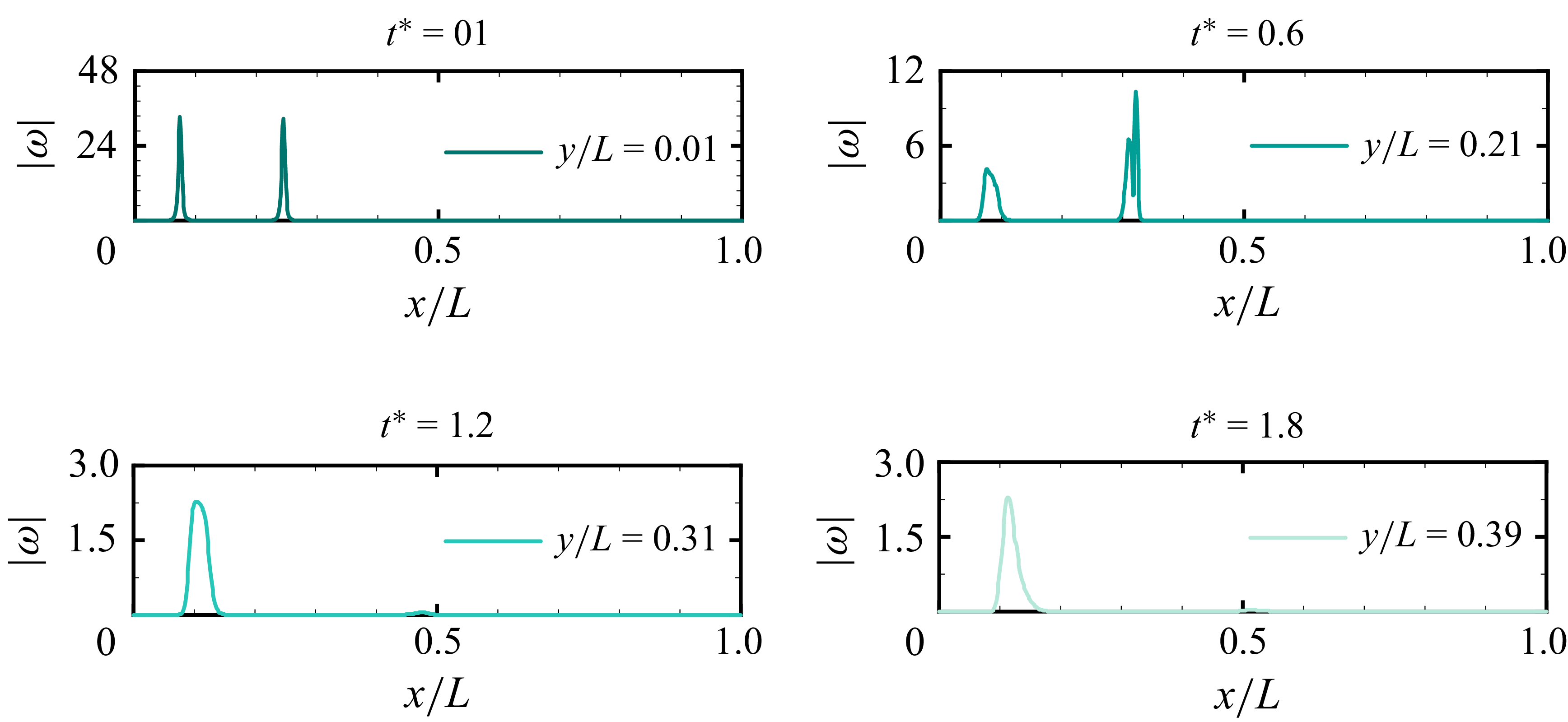
We further examine the spatial extent of the vorticity field near the computational boundaries during the reconnection process. Figure 16 shows profiles of the vorticity magnitude
 $ |\boldsymbol{\omega }|$
sampled along the
 $x$
-direction on the mid-plane
 $z=0.5L$
. The sampling lines are selected at different transverse locations and times, namely
 $y/L=0.01$
at
 $t^*=0.0$
,
 $y/L=0.21$
at
 $t^*=0.6$
,
 $y/L=0.31$
at
 $t^*=1.2$
, and
 $y/L=0.39$
at
 $t^*=1.8$
, to track the distribution of vorticity during the evolution.
The results show that large values of
 $ |\boldsymbol{\omega }|$
appear mainly as localised peaks associated with the vortex cores and interfacial structures. Away from these regions, the vorticity decays rapidly to a low background level. No clear high-vorticity region or vorticity accumulation is observed near the periodic boundaries at the examined stages. These observations indicate that the regions of appreciable vorticity remain localised and well separated from the periodic boundaries over the time interval considered.
Appendix B. Validation of the surface-tension model
To validate the surface-tension model, we compare our results with the reference data reported by Liu et al. (Reference Liu, Ng, Chong, Lohse and Verzicco2021). Figure 17(a) shows the three-dimensional interface evolution from the present simulation. Figure 17(b) compares the projected cross-sectional bubble shape on the
 $x$
–
 $z$
plane with the benchmark results of Sussman & Smereka (Reference Sussman and Smereka1997), Ding et al. (Reference Ding, Spelt and Shu2007) and Liu et al. (Reference Liu, Ng, Chong, Lohse and Verzicco2021). The test case concerns the rise of a single spherical bubble in a quiescent liquid under gravity. The computational domain is a cube of side length
 $8R_b$
, where
 $R_b$
is the initial bubble radius. The bubble centre is initially located at height
 $1.6R_b$
from the bottom boundary.
The density and viscosity ratios are
 $\lambda _{\rho } = \rho _g / \rho _l = 0.001$
and
 $\lambda _{\mu } = \mu _g / \mu _l = 0.01$
. With the characteristic velocity
 $U = \sqrt {gR_b}$
, the Reynolds number is
 $\textit{Re} = \rho _l U R_b / \mu _l = 100$
, and the Bond number is
 $\textit{Bo} = \rho _l g R_b^2 / \sigma = 200$
.
The interface shapes obtained in the present simulations agree well with the reference solutions of Sussman & Smereka (Reference Sussman and Smereka1997), Ding et al. (Reference Ding, Spelt and Shu2007) and Liu et al. (Reference Liu, Ng, Chong, Lohse and Verzicco2021), confirming that the surface-tension model accurately captures the interfacial dynamics of buoyancy-driven bubble motion.
Schematic of the toroidal bubble-ring configuration. Here,
 $R$
is the major radius, and
 $r$
is the minor radius.

Initialisation of the staggered velocity field for the two bubble rings.

Appendix C. Initial conditions for bubble-ring simulations
The initial velocity field for each bubble ring is prescribed using the RM vortex filament model. The toroidal geometry is characterised by the major radius
 $R$
and the tube radius
 $r$
, as illustrated in figure 18. On the Eulerian grid, the continuous RM integral (2.11) is evaluated in discretised form as
 \begin{equation} \boldsymbol{u}(\boldsymbol{x}) = \sum _{l=1}^{M_e} -\frac {\varGamma }{4\pi } \frac {(\boldsymbol{x} - \boldsymbol{x}_l) \times (\boldsymbol{T}_l\, \Delta s)}{\left ( \mathrm{e}^{-3/2}\,r^2 + |\boldsymbol{x} - \boldsymbol{x}_l|^2 \right )^{3/2}}, \end{equation}
where
 $\boldsymbol{x}$
and
 $\boldsymbol{x}_l$
are the positions of the Eulerian face centre and the
 $l$
th vortex element, respectively, and
 $\boldsymbol{T}_l\, \Delta s$
approximates the local tangent vector multiplied by the segment length. The vortex-ring centreline is discretised into
 $M_e = 2000$
Lagrangian elements, and the core desingularisation length scale is set to
 $ r$
, so that the vortex core scale remains comparable to the bubble-ring tube radius.
Initialisation of the liquid volume fraction and material properties.

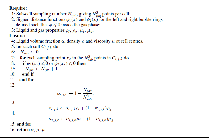
The initial interface is captured using a sub-grid supersampling technique. For each computational cell, the liquid volume fraction
 $\alpha$
is determined by sampling points within the cell. Assuming that the torus is centred at
 $\boldsymbol{x}_c = (x_c, y_c, z_c)$
with its symmetry axis aligned with the
 $y$
-axis, the signed distance function
 $\phi$
for a sampling point
 $\boldsymbol{x}$
is
 \begin{equation} \phi (\boldsymbol{x}) = \sqrt {\left (\sqrt {(x-x_c)^2 + (z-z_c)^2} - R\right )^2 + (y-y_c)^2} - r. \end{equation}
The volume fraction is then calculated as the ratio of sampling points in the gas phase where
 $\phi \leqslant 0$
. The complete initialisation procedure is summarised in algorithms 1 and 2, which describe the initialisation of the staggered velocity field and the cell-centred material fields, respectively.

 L
 R1=0.085L
 R2=0.11L
 r=0.0086L

 α=0.5
 t∗=0,0.3,0.6,0.9,1.2,1.5,1.8
 We=30.7
 We=3.07
 We=1.54

 x
 χ∗
 t∗=0

 α=0.5
 We=307
 We=3.07
 z=L/2
 |ω|

 We=3.07
 α=0.5
 |ω|=2

 t∗=0.6
 |ω|=3.5

 z
 We=30.7
 We=3.07

 x
 z
 x
 y
 We=30.7
 We=3.07
 We
 We
 We
 1%
 Ng
 rc∗(X∗,Y∗)

 z
 Ar∗
 We=3.07
 30.7
 307

 A∗
 κ∗

 We
 Ek∗
 Eki∗
 Ω∗
 ε∗

 V−
 H−∗

 t∗=1.5
 us∗
 We
 t∗=1.54
 us∗
 We

 We=3.07
 ρl/ρg=1000
 μl/μg=100
 Ek/Ek,0
 N=256
 512
 768
 α=0.5
 N=256
 512
 768
 |ω|
 x
 z=0.5L
 (y/L,t∗)
 (0.01,0.0)
 (0.21,0.6)
 (0.31,1.2)
 (0.39,1.8)

 x
 z
 t∗=0
 0.8
 1.2
 1.6
 t∗=0
 t∗=1.2

 R
 r