
1. Introduction
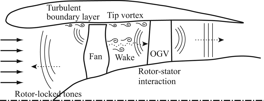
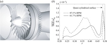
For the current commercial jet airplanes, fan noise becomes one of the major components of the community noise from approach to take-off conditions (Envia Reference Envia2002a; Burley et al. Reference Burley, Rawls, Berton and Marcolini2012; Huff Reference Huff2013; Leylekian, Lebrun & Lempereur Reference Leylekian, Lebrun and Lempereur2014). The fan noise from a turbofan engine consists of several noise-generation mechanisms including the rotor–stator interaction over the entire engine speed, the rotor-locked tones emitted at supersonic fan-tip speeds and other broadband noise sources, such as the interaction between the wall boundary layer and the rotor tip as well as the interaction between the boundary layer over the blade surface and the trailing edge (see figure 1). The rotor–stator interaction itself comprises (i) wakes and tip vortices originated from the rotor, (ii) unsteady stator responses to them and (iii) resultant sound radiated upstream and downstream via sound propagation/reflection/transmission through the duct and the blade rows. The information about the balance of these fan-noise-source contributions is important to strategize the liner design in engine nacelles and to model the noise sources for the fan-noise prediction. However, it is non-trivial to isolate each noise source either computationally or experimentally; accordingly, their relative importance as a function of the engine speed is still controversial.
Schematic diagram illustrating major fan-noise sources.

In recent numerical studies (Pérez Arroyo et al. Reference Pérez Arroyo, Leonard, Sanjose, Moreau and Duchaine2016; Shur et al. Reference Shur, Strelets, Travin, Spalart and Suzuki2018c; Suzuki et al. Reference Suzuki, Spalart, Shur, Strelets and Travin2018; Kholodov, Sanjose & Moreau Reference Kholodov, Sanjose and Moreau2020; Francois, Polacsek & Barrier Reference Francois, Polacsek and Barrier2022), the importance of unsteady motions originated near the fan-blade tip has been paid attention, and their interaction with the outlet guide vanes (OGVs) has been investigated in the context of fan broadband noise. In particular, streamwise vortical structures evolving near the outer wall seem to be related to a substantial part of the rotor–stator interaction noise. In this regard, an axial-velocity deficit in the outer-wall boundary layer behind the rotor should be highlighted. If the flow angle behind the fan is assumed to be aligned with the fan-blade trailing-edge angle  $\beta$, the azimuthal velocity
 $V$ can be related to the axial velocity
 $U$ in the frame moving with the rotor angular speed
 $\varOmega$ as a function of the radius
 $r$ as
 \begin{equation} V \left( r \right) \approx \varOmega r + \tan \left[\beta \left( r \right) - \Delta \beta \right] U \left( r \right) , \end{equation}
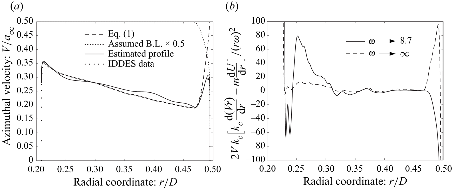
where  $\Delta \beta$ denotes the deviation flow angle from the blade trailing-edge angle. Figure 2(a) compares the estimated azimuthal-velocity profile with the actual simulation profile (Suzuki et al. Reference Suzuki, Shur, Strelets and Travin2022) at a low-speed/approach condition of NASA's high-speed fan rig, called source diagnostic test (SDT) (Hughes et al. Reference Hughes, Jeracki, Woodward and Miller2002) designed by General Electric, by assuming
 $\Delta \beta = 2^{\circ }$. Here, we have averaged the velocity components in time and the azimuthal direction at
 $x/D \approx 0.13$, which is right behind the rotor; subsequently, we have multiplied (1.1) by a turbulent boundary-layer profile on the outer wall (the log-law profile with
 $90\,\%$ reduced friction velocity plus the wake profile by Hinze Reference Hinze1959). The key takeaway is that a sharp peak near the outer wall is inevitably created behind the rotor in the azimuthal-velocity profile.
Mean-flow characteristics in the interstage. Velocity profiles are taken from the IDDES at an approach condition ( $61.7\,\%$ RPM). (a) Comparison of the azimuthal mean-velocity profiles. (b) Stability criterion (6.1) in Heaton & Peake (Reference Heaton and Peake2006) for
 $m = 22$.

Such a pointy mean-velocity profile seems to invoke hydrodynamic instabilities in the interstage region: the combination of the axial- and azimuthal-velocity profiles can break the generalized Rayleigh's stability criterion for a parallel swirling flow proposed by Heaton & Peake (Reference Heaton and Peake2006) from low to mid frequencies. Figure 2(b) plots their metric at a low frequency (corresponding to the peak of the second unstable regime explained below) and at the high-frequency asymptote, which is mostly positive (i.e. stable) except for a very thin layer near the outer wall. Our previous study (Suzuki et al. Reference Suzuki, Shur, Strelets and Travin2022) discovered two types of instabilities using the interstage velocity profile based on incompressible linear stability analysis: the first regime becomes unstable over wide frequencies including the rotor speed, forming wavepacket-like structures above the outer-wall boundary layer. The second unstable regime excites disturbances very close to the outer wall at much lower frequencies with smaller axial wavenumbers. This study has shown that coherent structures extracted from a turbulence-resolved simulation, referred to as improved delayed detached-eddy simulation (IDDES), possess properties similar to those predicted by the linear stability analysis. Our linear stability analysis of a different fan rig, called advanced ducted propulsor (ADP), designed by Pratt & Whitney, has found similar unstable regimes (Suzuki et al. Reference Suzuki, Shur, Strelets and Travin2021). Thus, it is highly possible that such instabilities are commonly excited in the interstage of turbomachinery due to the nature of the velocity field behind the rotor.
In the old days, hydrodynamic instabilities between coaxial cylinders have been investigated as Taylor–Couette flow with axial velocity or lately referred to as spiral Poiseuille flow for many engineering applications (Diprima Reference Diprima1960; Chandrasekhar Reference Chandrasekhar1961; Takeuchi & Jankowski Reference Takeuchi and Jankowski1981; Ng & Turner Reference Ng and Turner1982), and several flow regimes have been discovered at relatively low Reynolds numbers (Kaye & Elgar Reference Kaye and Elgar1958; Lueptow, Docter & Min Reference Lueptow, Docter and Min1992; Murai et al. Reference Murai, Tasaka, Oishi and Takeda2018). More recently, acoustic wave propagation together with spiral annulus-flow instabilities has also been analysed (Golubev & Atassi Reference Golubev and Atassi1998; Tam & Auriault Reference Tam and Auriault1998; Heaton & Peake Reference Heaton and Peake2006). In these studies, however, the velocity profiles are mostly laminar or transient, and at least one of the walls is rotating and driving the swirl velocity. Our focus is the instabilities rather in high-Reynolds-number interstage flows of turbomachinery, in which both walls are mostly stationary. Our previous study (Suzuki et al. Reference Suzuki, Shur, Strelets and Travin2022) numerically investigated such a flow by simulating the SDT fan rig, and successfully extracted coherent structures resembling such instability waves using an approach equivalent to dynamic mode decomposition (DMD, Schmid Reference Schmid2010). A successive study (Suzuki et al. Reference Suzuki, Shur, Strelets and Travin2021) analysed a higher engine-speed condition including ADP fan rig. However, these previous studies covered limited engine speeds and compared with linear stability analysis only for incompressible flow.
As mentioned above, the series of instability analyses on the interstage flow was originally motivated by the fan broadband noise from the inlet, which is predominated by co-rotating azimuthal modes along the inner side of the cut-on line (refer to figure 24 shown later). Such a ‘biased’ modal distribution seems to be collapsed toward the cut-on line with increasing engine speed. This trend can be observed by the mode-ring measurement in the SDT (see figure 4 in Premo & Joppa Reference Premo and Joppa2002) as well as the simulations (Suzuki et al. Reference Suzuki, Spalart, Shur, Strelets and Travin2019) covering a supersonic fan-tip Mach number at a take-off condition ( $100\,\%$ RPM). In fact, analogous stripes along the cut-on line were found in the IDDES at an approach condition (
 $61.7\,\%$ RPM), and a potential noise-generation mechanism associated with the aforementioned instabilities was discussed by Suzuki et al. (Reference Suzuki, Shur, Strelets and Travin2022): in addition to the amplification of vortical disturbances near the outer wall via these hydrodynamic instabilities, additional broadband noise may be generated by the interaction of coherent structures invoked by one of these instabilities with turbulence in the rotor wakes. Now, the interest is how such instability characteristics change over a range of the operating condition, and how they potentially influence the fan noise at transonic fan-tip Mach numbers.
The objective is to expand the investigation on the instability analysis of the turbomachinery interstage flow by focusing on the engine speed and on the relation to the fan broadband noise. In this study, compressible linear stability analysis is applied over a wide range of engine speed: by taking the velocity profiles from NASA's SDT fan rig, the stability characteristics are analysed at approach, cut-back and take-off conditions. Moreover, the past IDDES data solving the SDT geometry are post-processed using an approach equivalent to DMD at the approach and the cut-back conditions, and the characteristics of the extracted coherent structures are compared with those predicted by the linear stability analysis. Since the compressibility is included in this analysis, acoustic modes coexisting with hydrodynamic unstable modes can be identified using realistic velocity profiles. Thus, the relation of these instability waves with the rotor–stator interaction noise can be investigated. Furthermore, mode distributions in the interstage are analysed by focusing on pressure fluctuations on the outer wall. Throughout these analyses, a fan-noise generation mechanism associated with nonlinear interaction between two different types of coherent structures is supported rather than interaction between acoustic and hydrodynamic disturbances.
The rest of the paper is organized as follows. After the introduction, the SDT fan rig and the test conditions are briefly reviewed, and the numerical methods of the IDDES and its database are summarized. The Taylor–Couette-/spiral-Poiseuille-flow instability is then introduced by focusing on compressible flow, and the instability characteristics are compared between compressible and incompressible flows by using a spectral method. Subsequently, the post-processing results using the IDDES database are discussed: (i) hydrodynamic modes and their dispersion relations of velocity disturbances extracted from the IDDES are compared with those derived from the linear stability analysis; (ii) duct acoustic modes are investigated by decomposing the outer-wall pressure fluctuations; and (iii) the potential contributions of such an instability phenomenon to the fan noise are considered. Conclusions are finally summarized, followed by the Appendix providing the comparison of the IDDES results with the experimental data.
2. Testbed: SDT
A series of aerodynamic and aeroacoustic tests using the aforementioned model-scale fan rig, called the SDT, was conducted in the  $9' \times 15'$ low-speed wind tunnel at the NASA Glenn Research Center, and the test results were reported by Hughes et al. (Reference Hughes, Jeracki, Woodward and Miller2002), Woodward et al. (Reference Woodward, Hughes, Jeracki and Miller2002), Heidelberg (Reference Heidelberg2002), Premo & Joppa (Reference Premo and Joppa2002), Envia (Reference Envia2002b) and Podboy et al. (Reference Podboy, Krupar, Hughes and Woodward2002). This fan rig with
 $D = 22''$ (
 $= 0.5588$ m) diameter was equipped with a rotor and a stator in an axisymmetric hard-wall nacelle without a pylon/bifurcation or core flow. The tunnel Mach number was set to be
 $M_{\infty } = 0.1$. Among several tested configurations, the baseline geometry, consisting of
 $22$ fan blades (called R4) and
 $54$ unswept OGVs, is investigated throughout this study. Three engine speeds, one representing an approach condition (
 $61.7\,\%$ RPM, i.e.
 $7,809$ RPM), the other a cut-back condition (
 $87.5\,\%$ RPM, i.e.
 $11\,074$ RPM) and the last a take-off condition (
 $100\,\%$ RPM, i.e.
 $12,657$ RPM) are studied, the corresponding blade-passing frequencies (BPF) being
 $f_{{BPF}} = 2,863$ Hz,
 $4,060$ Hz and
 $4,641$ Hz, respectively. These numbers are summarized in table 1. For the post-processing of the numerical database, the first two engine speeds are investigated.
Operating conditions of different engine speeds for SDT.

3. Summary of the computational fluid dynamics (CFD) method and database
An in-house code, called ‘Numerical Turbulence Simulation’, developed by Shur et al. (Reference Shur, Spalart, Strelets and Travin2008), was designed to predict both fan tones and broadband noise associated with the rotor–stator interaction by simulating the SDT geometry. A series of the aerodynamic and aeroacoustic results has been reported in Shur et al. (Reference Shur, Strelets, Travin, Spalart and Suzuki2018c), Suzuki et al. (Reference Suzuki, Spalart, Shur, Strelets and Travin2018) and Suzuki et al. (Reference Suzuki, Spalart, Shur, Strelets and Travin2019), together with details of the numerical methods including the turbulence treatments, the grid design and the acoustic extraction/projection. The summary of the numerical methods and the points relevant to this study are reviewed below.
The SDT geometry including the entire nacelle was solved using the zonal unsteady Reynolds-averaged Navier–Stokes (URANS) wall-modelled large eddy simulation approach based on IDDES (simply called IDDES hereafter) was taken together with the volume synthetic turbulence generator (VSTG, refer to Shur et al. Reference Shur, Strelets, Travin, Probst, Probst, Schwamborn, Deck, Skillen, Holgate and Revell2018a). This technique was achieved by tailoring spatially distributed unsteady source terms in the momentum and subgrid turbulent-kinetic-energy transport equations. The VSTG was activated in a relatively narrow region right downstream of the fan trailing edge to trigger the scale-resolving capability of the IDDES in the interstage and farther downstream. All the empirical constants and parameters entering the VSTG had been determined by Shur et al. (Reference Shur, Spalart, Strelets and Travin2014) and Shur et al. (Reference Shur, Strelets, Travin, Probst, Probst, Schwamborn, Deck, Skillen, Holgate and Revell2018a) based on the computation of three canonical turbulent shear flows (developed channel flow, zero pressure gradient boundary layer and plane mixing layer), and they have been used in the series of the fan-flow computations with no further adjustment. To properly simulate the modal contents for the stability analysis, the random-number generator used for the synthetic velocity fluctuations in the source terms was specifically tailored: their wavenumber distribution smoothly diminishes beyond the cut-off, which corresponds to  $m \approx \pm 39$ and
 $\pm 57$ at the approach and cut-back conditions, respectively. These active wavenumbers approximately cover the unstable azimuthal-mode range of the second unstable regime, plotted in figure 17 later. Suzuki et al. (Reference Suzuki, Shur, Strelets and Travin2022) documented this upgraded VSTG in details.
The entire SDT geometry including the fan blades, the OGVs, the bypass duct and the nacelle over  $360^{\circ }$ was gridded with multi-block structured meshes of the Chimera type, distributing a total of approximately
 $140$ or
 $170$ million cells at the approach or cut-back condition, respectively. The block including the rotor and its fore- and aft-adjacent blocks were rotated together and communicated with the rest of the stationary blocks with a sliding-interface technique (refer to Shur et al. Reference Shur, Strelets, Travin, Christophe, Kucukcoskun, Schram, Sack and Åbom2018b). The grids in the vicinity of the rotor were aligned with the fan trailing edges and clustered in the wakes (the azimuthal cell count is no less than
 $12$); subsequently, they were smoothly transitioned to a uniform azimuthal distribution (
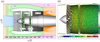
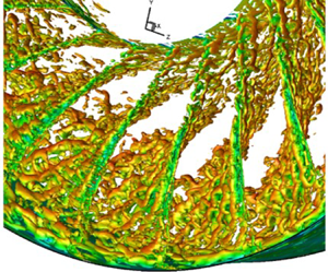
 $36$ cells between the fan-blade passage) in the middle of the interstage and farther downstream. With such a grid design, combined with the weighted fourth-order centred/fifth-order upwind-biased scheme for the inviscid gasdynamic fluxes, turbulence in the interstage was resolved with sufficient accuracy. The computational mesh and an instantaneous vorticity field are displayed in figure 3.
Computational domain of the IDDES. (a) Computational mesh (every other point in  $x$ and
 $y$) and their azimuthal grid counts. (b) Vorticity field at
 $61.7\,\%$ RPM.

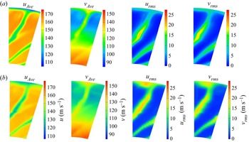
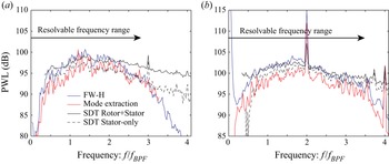
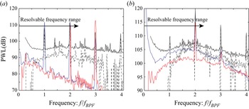
In Shur et al. (Reference Shur, Strelets, Travin, Spalart and Suzuki2018c) and Suzuki et al. (Reference Suzuki, Spalart, Shur, Strelets and Travin2018, Reference Suzuki, Spalart, Shur, Strelets and Travin2019), aerodynamic and aeroacoustic results of the IDDES at the approach and take-off conditions have been validated against the SDT experimental data, and the limitations have also been discussed. In the Appendix, the flow field at the cut-back condition simulated by the IDDES with the upgraded VSTG is similarly validated with the LDV data. The radiated sound-power-level (PWL) spectra in the inlet and the exhaust are also compared with traverse microphone data of the SDT to demonstrate the validity of the IDDES database.
4. Taylor–Couette-/spiral-Poiseuille-flow instability
4.1. Systems of the equations and the spectral method
In this study, linear stability analysis is performed for both incompressible and compressible flows to evaluate the compressibility effects. The procedure for incompressible flows was documented in the aforementioned study (Suzuki et al. Reference Suzuki, Shur, Strelets and Travin2022); accordingly, the procedure for compressible flows is mainly formulated in the rest of this section. For both problems, the approach taken by Takeuchi & Jankowski (Reference Takeuchi and Jankowski1981) is essentially followed: the Navier–Stokes equations are linearized by assuming axisymmetry of the mean flow as well as homogeneity in the axial direction, and eigenvalue problems are solved using a spectral method with the Chebyshev polynomials (Orszag Reference Orszag1971). The axial and azimuthal mean-velocity profiles, expressed as  $U(r)$ and
 $V(r)$ respectively, are taken from the aforementioned IDDES (Suzuki et al. Reference Suzuki, Shur, Strelets and Travin2022) approximately at the middle of the interstage,
 $x/D \approx 0.18$ of the SDT geometry. Here,
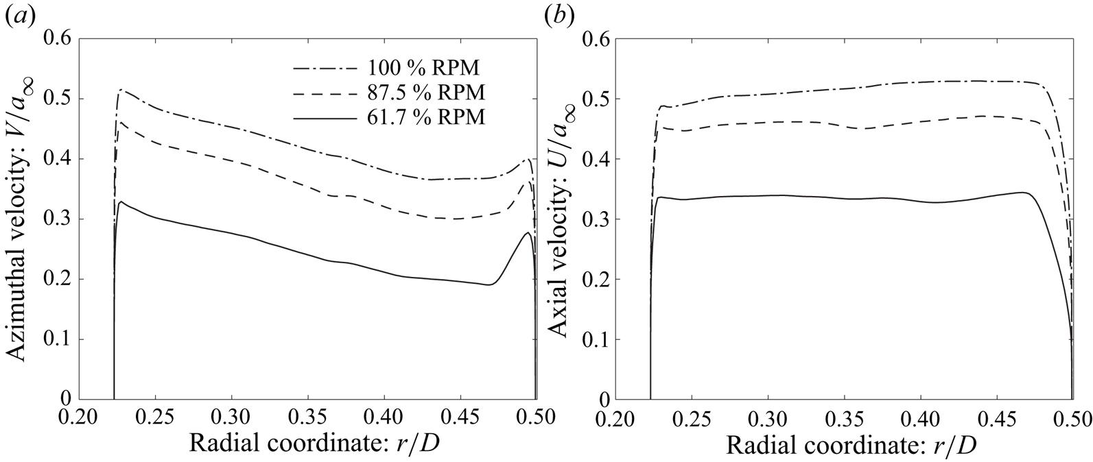
 $x = 0$ is taken at the fan-blade pitch axis, as shown in figure 3. These velocity profiles at three engine speeds are compared in figure 4, highlighting that the azimuthal-velocity peak is most pronounced at the approach condition for the SDT. For compressible flows, the mean density and temperature profiles, expressed as
 $\rho (r)$ and
 $T(r)$ respectively, are additionally taken from the IDDES. Since all these profiles including the thermodynamic quantities are assumed to be invariant in the axial direction, the axial pressure gradient is accordingly neglected; namely, the viscous effect generating the axial pressure gradient is assumed to be much smaller than the radial variation and other terms.
Mean-velocity profiles in the interstage of SDT at three engine speeds (normalized by the ambient speed of sound) at  $x/D \approx 0.18$ computed by the IDDES. (a) Azimuthal velocity. (b) Axial velocity.

4.2. Temporal analysis and neutrally stable boundaries
The compressible Navier–Stokes equations are non-dimensionalized by using the ambient density and speed of sound for the air, expressed as  $\rho _{\infty }$ and
 $a_{\infty } = \sqrt {\gamma R T_{\infty }}$ (
 $= 1.226\,{\rm kg}\,{\rm m}^{-3}$ and
 $340.2\,{\rm m}\,{\rm s}^{-1}$ in this study) respectively, as well as the fan diameter
 $D$ (
 $= 0.5588$ m). By expressing small flow perturbations as
 $\hat {f} ( r ) \exp [ - {\rm i} ( \omega t - k_x x - m \phi ) ]$, where
 $\omega$,
 $k_x$ and
 $m$ respectively denote the angular frequency, the axial wavenumber and the azimuthal-mode number, a system of the non-dimensional linearized equations in the Fourier domain is written in the cylindrical coordinates as (the corresponding system for an incompressible flow can be found in Suzuki et al. Reference Suzuki, Shur, Strelets and Travin2022)
 \begin{align} &{\rm i} k_x \hat{u} + {\rm i} \frac{m}{r} \hat{v} + \left( \frac{\partial}{\partial r} + \frac{1}{r} + \frac{1}{\rho} \frac{\partial \rho}{\partial r} \right) \hat{w} + {\rm i} \frac{1}{\rho} \left( \frac{m V}{r} + k_x U \right) \hat{\rho} = {\rm i} \omega \frac{1}{\rho} {\hat \rho},\\ \end{align}
 \begin{align} &\left[ {\rm i} \left( \frac{m V}{r} + k_x U \right) - \frac{\mu Ma}{\rho Re} \left( \Delta - \frac{k_x^2}{3} + \frac{{\rm d} \mu}{{\rm d} T} \frac{\partial T}{\partial r} \frac{\partial}{\partial r} \right) \right] \hat{u} \nonumber\\ &\qquad + \frac{k_x m \mu Ma}{3 r \rho Re} \hat{v} + \left[ \frac{\partial U}{\partial r} - {\rm i} \frac{k_x \mu Ma}{\rho Re} \left( \frac{1}{3} \frac{\partial }{\partial r} + \frac{1}{3r} + \frac{{\rm d} \mu}{{\rm d} T} \frac{\partial T}{\partial r} \right) \right] \hat{w} \nonumber\\ &\qquad + {\rm i} \frac{k_x T}{\gamma \rho} \hat{\rho} + \left[ {\rm i} \frac{k_x}{\gamma} - \frac{\mu Ma}{\rho Re} \frac{{\rm d} \mu}{{\rm d} T} \left( \frac{\partial U}{\partial r} \frac{\partial}{\partial r} + \frac{\partial^2 U}{\partial r^2} + \frac{1}{r} \frac{\partial U}{\partial r} \right) \right] \hat{T} = {\rm i} \omega \hat{u},\\ \end{align}
 \begin{align} & \frac{k_x m \mu Ma}{3 r \rho Re} \hat{u} \nonumber\\ &\qquad + \left[ {\rm i} \left(\frac{m V}{r} + k_x U\right) - \frac{\mu Ma}{\rho Re} \left\{ \Delta - \frac{1}{r^2} - \frac{m^2}{3 r^2} + \frac{{\rm d} \mu}{{\rm d} T} \frac{\partial T}{\partial r} \left( \frac{\partial}{\partial r} - \frac{1}{r} \right) \right\} \right] \hat{v} \nonumber\\ &\qquad + \left[ \left( \frac{\partial V}{\partial r} + \frac{V}{r} \right) - {\rm i} \frac{m \mu Ma}{r \rho Re} \left( \frac{7}{3r} + \frac{1}{3} \frac{\partial}{\partial r} + \frac{{\rm d} \mu}{{\rm d} T} \frac{\partial T}{\partial r} \right) \right] \hat{w} + {\rm i} \frac{m T}{\gamma \rho r} {\hat \rho} \nonumber\\ &\qquad + \left[ {\rm i} \frac{m}{\gamma r} - \frac{\mu Ma}{\rho Re} \frac{{\rm d} \mu}{{\rm d} T} \left\{ \left( \frac{\partial V}{\partial r} - \frac{V}{r} \right) \frac{\partial}{\partial r} + \left( \frac{\partial^2 V}{\partial r^2} + \frac{1}{r} \frac{\partial V}{\partial r} \right) \right\} \right] \hat{T} = {\rm i} \omega \hat{v},\\ \end{align}
 \begin{align} &- {\rm i} \frac{k_x \mu Ma}{3 \rho Re} \left( \frac{\partial}{\partial r} - 2 \frac{{\rm d} \mu}{{\rm d} T} \frac{\partial T}{\partial r} \right) \hat{u} \nonumber\\ &\qquad - \left[ \frac{2~V}{r} - {\rm i} \frac{m \mu Ma}{3 r \rho Re} \left( \frac{7}{r} - \frac{\partial }{\partial r} + 2 \frac{{\rm d} \mu}{{\rm d} T} \frac{\partial T}{\partial r} \right) \right] \hat{v} \nonumber\\ &\qquad + \left[ {\rm i} \left( \frac{m V}{r} + k_x U \right) \right.\nonumber\\ &\left.\qquad - \frac{\mu Ma}{\rho Re} \left\{ \Delta + \frac{1}{3} \frac{\partial^2}{\partial r^2} + \frac{1}{3r} \frac{\partial}{\partial r} - \frac{4}{3 r^2} + \frac{2}{3} \frac{{\rm d} \mu}{{\rm d} T} \frac{\partial T}{\partial r} \left( 2 \frac{\partial}{\partial r} - \frac{1}{r} \right) \right\} \right] \hat{w} \nonumber\\ &\qquad + \frac{1}{\gamma \rho} \left( T \frac{\partial }{\partial r} + \frac{\partial T }{\partial r} \right) \hat{\rho} \nonumber\\ &\qquad + \left[ \frac{1}{\gamma} \left( \frac{\partial }{\partial r} + \frac{1}{\rho} \frac{\partial \rho}{\partial r} \right) - \frac{\mu Ma}{\rho Re} \frac{{\rm d} \mu}{{\rm d} T} \left\{ {\rm i} \frac{m}{r} \left( \frac{\partial V}{\partial r} - \frac{V}{r} \right) + {\rm i} k_x \frac{\partial U}{\partial r} \right\} \right] \hat{T} = {\rm i} \omega \hat{w},\\ \end{align}
 \begin{align} & -\frac{2 \gamma \mu Ma}{\rho Re} \frac{\partial U}{\partial r} \frac{\partial}{\partial r} \hat{u} - \frac{2 \gamma \mu Ma}{\rho Re} \left( \frac{\partial V}{\partial r} - \frac{V}{r} \right) \left( \frac{\partial }{\partial r} - \frac{1}{r} \right) \hat{v} \nonumber\\ &\qquad + \left[ \frac{1}{\gamma - 1} \frac{\partial T}{\partial r} - \frac{T}{\rho} \frac{\partial \rho}{\partial r} - {\rm i} \frac{2 \gamma \mu Ma}{\rho Re} \left\{ k_x \frac{\partial U}{\partial r} + \frac{m}{r} \left( \frac{\partial V}{\partial r} - \frac{V}{r} \right) \right\} \right] \hat{w} \nonumber\\ &\qquad - {\rm i} \frac{T}{\rho} \left( \frac{m V}{r} + k_x U \right) \hat{\rho} \nonumber\\ &\qquad + \frac{{\rm i}}{\gamma - 1} \left[ \left( \frac{m V}{r} + k_x U \right) + \frac{{\rm i} \gamma \mu Ma}{\rho Re Pr} \left\{ \Delta +\frac{{\rm d} \mu}{{\rm d} T} \left( \frac{\partial^2~T}{\partial r^2} + \frac{1}{r} \frac{\partial T}{\partial r} + 2 \frac{\partial T}{\partial r} \frac{\partial}{\partial r} \right) \right.\right.\nonumber \\ &\left.\left.\qquad + \left( \gamma - 1 \right) Pr \frac{{\rm d} \mu}{{\rm d} T} \left( \left( \frac{\partial U}{\partial r} \right)^2 + \left( \frac{\partial V}{\partial r} - \frac{V}{r} \right)^2 \right) \right\} \right] \hat{T} = {\rm i} \omega \left[ \frac{\hat{T}}{\gamma - 1} - \frac{T}{\rho} \hat{\rho} \right], \end{align}
where  $\hat {u}$,
 $\hat {v}$ and
 $\hat {w}$ denote the axial-, azimuthal- and radial-velocity components of the perturbation, respectively, and
 $\hat {\rho }$ and
 $\hat {T}$ the density and temperature perturbations, respectively. The Reynolds number, the Prandtl number and the Mach number are defined as
 $Re \equiv \rho _{\infty } \bar {U} D / \bar {\mu }$,
 $Pr \equiv \gamma R \bar {\mu } / (\gamma - 1 ) \bar {\kappa } = 0.72$ and
 $Ma \equiv \bar {U} / a_{\infty }$, where the gas constant
 $R$ is assumed to be constant; moreover, the quantities with the top bar are those averaged over the interstage station (refer to table 1 for
 $\bar {U}$ and
 $\bar {T}$ in each condition) only to characterize the Reynolds number. To include the temperature dependence of the dynamic viscosity
 $\mu$ and the heat conductivity
 $\kappa$, the Sutherland formula (Sutherland Reference Sutherland1893) is adopted (the dimensional formula is given below)
 \begin{equation} \mu = \frac{ 0.72 \left( \gamma - 1 \right)}{\gamma R} \kappa \equiv \mu_0 \left( \frac{T}{T_0} \right)^{1.5} \frac{T_0 + C}{T + C} , \end{equation}
where  $\mu _0 = 1.716 \times 10^{-5}$ kg (s m)
 $^{-1}$,
 $T_0 = 273.15$ K,
 $C = 110.5$ K, respectively. The same constants are used for the heat conductivity, as it is related by the Prandtl number defined above. The Laplacian in (4.1) is also defined as
 \begin{equation} \Delta \equiv \frac{\partial^2}{\partial r^2} + \frac{1}{r} \frac{\partial }{\partial r} - \frac{m^2}{r^2} - k_x^2 , \end{equation}
which is different from the notation by Takeuchi & Jankowski (Reference Takeuchi and Jankowski1981). On both sides of the walls, the no-slip boundary conditions are imposed for the three velocity components.
The equations above are cast such that the angular frequency  $\omega$ is linearly placed on the right-hand side and all the other terms on the left-hand side. Accordingly, temporal instability can be solved as a generalized eigenvalue problem using a spectral method developed by Orszag (Reference Orszag1971): using the Chebyshev polynomials, the system of the equation (4.1) is discretized in the radial direction into
 $N_p$ (
 $= 256$ in most cases) cells in a staggered manner (Macaraeg, Streett & Hussaini Reference Macaraeg, Streett and Hussaini1988). Namely, the three velocity components are located at
 $N_p+1$ grid points including the boundary points on the wall, while the density and the temperature are assigned at
 $N_p$ mid points; accordingly,
 $3 \times ( N_p+1 )$ equations for the momentum and
 $2 \times N_p$ equations for continuity and energy are solved in essence. Yet, six equations are sacrificed in the highest orders of these equations for the no-slip boundary conditions on both walls. Consequently, the total of
 $5N_p + 3$ equations are simultaneously solved for a compressible flow, as opposed to
 $4N_p + 3$ equations for an incompressible flow. It should be noted that the incompressible solver has been verified by comparing with the results reported by Takeuchi & Jankowski (Reference Takeuchi and Jankowski1981).
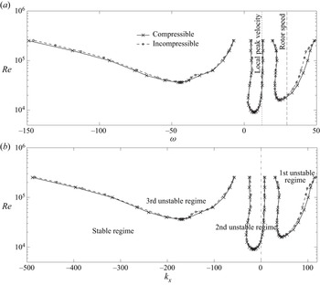
We begin with comparing the neutrally stable boundaries (the lines at which the most unstable growth rate vanishes) for incompressible and compressible solutions by solving this temporal problem (as the boundaries are common to a spatial problem). Figure 5 plots those for  $m = 22$ (which is the same as the fan-blade count as an example) at the approach condition up to the Reynolds number at which the current spectral code can resolve the eigenvalue problem (the Reynolds number of the SDT/IDDES is
 $Re \approx 4 \times 10^6$). The solutions for
 $m = -22$ become the mirror image of these figures (i.e. the signs of
 $\omega$ and
 $k_x$ are flipped). First, the boundaries for incompressible and compressible flows almost overlap each other, indicating negligible compressibility effects. Second, we find three distinct unstable regimes, as labelled in figure 5(b): the first regime becomes unstable over a relatively wide frequency range, and its boundary spreads with the Reynolds number. This mode can destabilize disturbances moving with the rotor speed, indicated by the dashed vertical line in figure 5(a), i.e. the rotating speed of the wakes given by
 $\omega = m \varOmega$. The second regime resides only within a narrow range of small axial wavenumbers at low frequencies, corresponding to the local peak azimuthal velocity or lower near the outer wall, i.e.
 $\omega \approx mV/r$, indicated by the dotted line. These two modes rotate in the direction of the rotor. The third regime becomes unstable at relatively higher Reynolds numbers but spreads its boundary very rapidly. This mode physically appears as a counter-rotating mode (i.e.
 $m = -22$ in this case) with the opposite sign for
 $\omega$ and
 $k_x$; hence, it can still convect downstream. As discussed later, the rotational direction of a disturbance is indistinguishable from snapshots of flow fields in post-processing unless we track the evolution in time.
Neutrally stable boundaries in the interstage of SDT for  $m = 22$ at
 $61.7\,\%$ RPM. (a) Frequency dependence. (b) Wavenumber dependence.

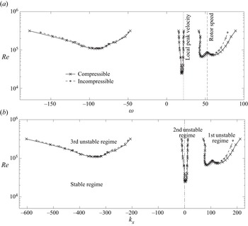
Figure 6 similarly compares the neutrally stable boundaries at the cut-back condition. It is clear that the compressibility is still negligible. We find similar three unstable regimes; to be precise, the second and the third regimes merge at higher Reynolds numbers, and the boundary of the first regime depicts a gentle double-hump shape. More importantly, the first unstable regime spreads over wider frequencies but migrates to a higher-frequency range beyond the rotor speed; in addition, the critical Reynolds number of the first regime becomes noticeably higher than that at the approach. This implies that disturbances in the wakes are less amplified compared with the lower speed. On the other hand, the second unstable regime hardly shifts the frequency range relative to the local azimuthal velocity, but its wavenumber range migrates to the negative side in contrast to the approach condition.
Neutrally stable boundaries in the interstage of SDT for  $m = 22$ at
 $87.5\,\%$ RPM. (a) Frequency dependence. (b) Wavenumber dependence.

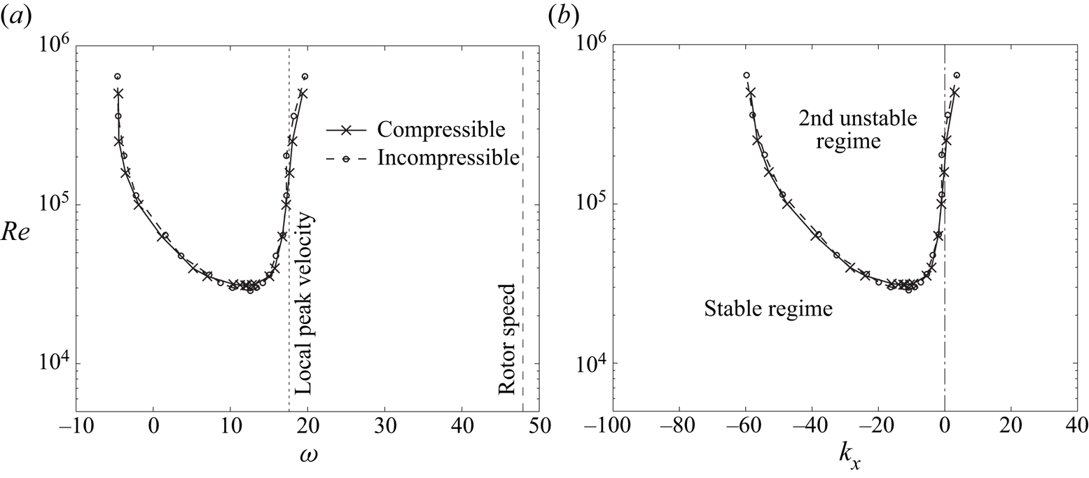
When the engine speed is increased to the take-off speed, the first and third regimes cannot be found up to the Reynolds-number range which this code can handle ( $Re \lesssim 5 \times 10^5$), even though unstable modes are searched over a wider range than the two previous lower engine speeds (i.e.
 $-600 \lesssim k_x \lesssim 500$). Presumably, the critical Reynolds numbers of these two regimes are even higher than the resolvable range, possibly because the peak of the azimuthal velocity is smeared at the take-off speed, as shown in figure 4. Figure 7 shows that the second unstable regime stays almost in the same
 $\omega$ and
 $k_x$ ranges as those at the cut-back condition. We also notice that the boundaries for incompressible and compressible flows still agree very well even at the full take-off speed (the tip Mach number of
 $M_{{ tip}} \approx 1.2$). Therefore, it is safe to conclude that the compressibility effect itself on the hydrodynamic instability is negligible in the interstage, while the velocity profiles, particularly in the azimuthal component, change with the engine speed, and the profile change has a greater impact on the instability characteristics.
Neutrally stable boundaries in the interstage of SDT for  $m = 22$ at
 $100\,\%$ RPM. (a) Frequency dependence. (b) Wavenumber dependence.

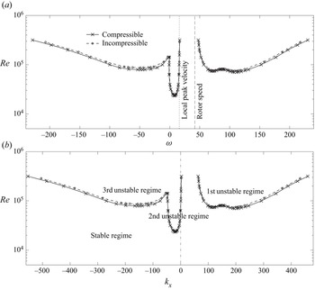
Figure 8 also plots the neutrally stable boundaries for  $m =39$ at the approach condition. This azimuthal-mode number is close to the upper threshold of the stripes associated with the fan broadband noise in this condition (refer to the discussion in Suzuki et al. Reference Suzuki, Shur, Strelets and Travin2022). While the critical Reynolds numbers for
 $m =39$ are higher in all the regimes, the three unstable regimes depict similar patterns to those for
 $m =22$ shown in figure 5 (interestingly, the first unstable regime depicts a clear double-hump shape even though processing the same velocity profiles as
 $m =22$). Thus, we still anticipate that the flow is unstable over the range of azimuthal modes mainly contained in the wake turbulence.
Neutrally stable boundaries in the interstage of SDT for  $m = 39$ at
 $61.7\,\%$ RPM. (a) Frequency dependence. (b) Wavenumber dependence.

We should remark that the second unstable regime stays close to the local peak velocity regardless of the engine speed or the azimuthal mode (refer to the  $\omega - Re$ plots from figures 5–8). This suggests that the pointy velocity profile near the outer wall drives the second unstable mode. On the other hand, the first regime becomes highly unstable at the rotor speed for both
 $m = 22$ and
 $39$, but only at the approach condition. Referring to the wave equation in the cylindrical coordinates (i.e. the Bessel equation), it may be possible to scale
 $\omega$ and
 $k_x$ proportionally with
 $m$ as a limit of a narrow annulus. Namely, the ranges of the unstable frequency and wavenumber shift approximately proportionally; as a result, these unstable ranges stay about the same relative to the rotor speed and the local azimuthal velocity at the approach condition. As the engine speed increases, the dispersion relation of
 $\mbox {Re}[ \omega ] - \mbox {Re}[ k_x ]$ retains the same similarity, but the unstable regime of the first instability shifts to higher frequencies relative to the rotor speed. Thus, the first unstable mode amplifies the wake disturbances less at higher engine speeds. We will closely observe the azimuthal-mode dependence in § 4.4.
4.3. Spatial analysis of instability waves and acoustic waves
Next, a spatial problem is solved to observe the dispersion relations and the eigenfunctions representative of a turbomachinery problem. Here, (4.1) is recast so that the axial wavenumber  $k_x$ is linearly placed on the right-hand side as
 \begin{align} & {\rm i} \frac{m}{r} \hat{v} + \left( \frac{\partial }{\partial r} + \frac{1}{r} + \frac{1}{\rho} \frac{\partial \rho}{\partial r} \right) \hat{w} + {\rm i} \frac{1}{\rho} \left( \frac{m V}{r} - \omega \right) \hat{\rho} ={-} {\rm i} k_x \left[ \hat{u} + \frac{U}{\rho} \hat{\rho} \right], \\\end{align}
 \begin{align} & \left[ {\rm i} \left( \frac{m V}{r} - \omega \right) - \frac{\mu Ma}{\rho Re} \left( \Delta - \frac{k_x^2}{3} + \frac{{\rm d} \mu}{{\rm d} T} \frac{\partial T}{\partial r} \frac{\partial}{\partial r} \right) \right] \hat{u} \nonumber\\ &\qquad + \frac{\partial U}{\partial r} \hat{w} - \frac{\mu Ma}{\rho Re} \frac{{\rm d} \mu}{{\rm d} T} \left( \frac{\partial U}{\partial r} \frac{\partial}{\partial r} + \frac{\partial^2~U}{\partial r^2} + \frac{1}{r} \frac{\partial U}{\partial r} \right) \hat{T} ={-} {\rm i} k_x \nonumber\\ & \left[U \hat{u} - {\rm i} \frac{m \mu Ma}{3 r \rho Re} \hat{v} - \frac{\mu Ma}{\rho Re} \left( \frac{1}{3} \frac{\partial }{\partial r} + \frac{1}{3r} + \frac{{\rm d} \mu}{{\rm d} T} \frac{\partial T}{\partial r} \right) \hat{w} + \frac{T}{\gamma \rho} \hat{\rho} + \frac{1}{\gamma} \hat{T} \right], \\\end{align}
 \begin{align} & \left[ {\rm i} \left( \frac{m V}{r} - \omega \right) - \frac{\mu Ma}{\rho Re} \left\{ \Delta - \frac{1}{r^2} - \frac{m^2}{3 r^2} + \frac{{\rm d} \mu}{{\rm d} T} \frac{\partial T}{\partial r} \left( \frac{\partial}{\partial r} - \frac{1}{r} \right) \right\} \right] \hat{v} \nonumber\\ &\qquad+ \left[ \left( \frac{\partial V}{\partial r} + \frac{V}{r} \right) - \frac{{\rm i} m \mu Ma}{r \rho Re} \left( \frac{7}{3r} + \frac{1}{3} \frac{\partial}{\partial r} + \frac{{\rm d} \mu}{{\rm d} T} \frac{\partial T}{\partial r} \right) \right] \hat{w} + {\rm i} \frac{m T}{\gamma r \rho} {\hat \rho} \nonumber\\ &\qquad+ \left[ {\rm i} \frac{m}{\gamma r} - \frac{\mu Ma}{\rho Re} \frac{{\rm d} \mu}{{\rm d} T} \left\{ \left( \frac{\partial V}{\partial r} - \frac{V}{r} \right) \frac{\partial}{\partial r} + \left( \frac{\partial^2~V}{\partial r^2} + \frac{1}{r} \frac{\partial V}{\partial r} \right) \right\} \right] \hat{T} ={-} {\rm i} k_x \nonumber\\ &\qquad\times \left[ -{\rm i} \frac{m \mu Ma}{3 r \rho Re} \hat{u} + U \hat{v} \right], \\\end{align}
 \begin{align} & - \left[ \frac{2V}{r} - {\rm i} \frac{m \mu Ma}{3 r \rho Re} \left( \frac{7}{r} - \frac{\partial }{\partial r} + 2 \frac{{\rm d} \mu}{{\rm d} T} \frac{\partial T}{\partial r} \right) \right] \hat{v} + \left[ {\rm i} \left( \frac{m V}{r} - \omega \right) \right.\nonumber\\ &\left.\qquad- \frac{\mu Ma}{\rho Re} \left\{ \Delta + \frac{1}{3} \frac{\partial^2}{\partial r^2} + \frac{1}{3r} \frac{\partial}{\partial r} - \frac{4}{3 r^2} + \frac{2}{3} \frac{{\rm d} \mu}{{\rm d} T} \frac{\partial T}{\partial r} \left( 2 \frac{\partial}{\partial r} - \frac{1}{r} \right) \right\} \right] \hat{w} \nonumber\\ &\qquad+ \frac{1}{\gamma \rho} \left( T \frac{\partial }{\partial r} + \frac{\partial T }{\partial r} \right) \hat{\rho} \nonumber\\ &\qquad+ \left[ \frac{1}{\gamma} \left( \frac{\partial }{\partial r} + \frac{1}{\rho} \frac{\partial \rho}{\partial r} \right) - {\rm i} \frac{m \mu Ma}{r \rho Re} \frac{{\rm d} \mu}{{\rm d} T} \left( \frac{\partial V}{\partial r} - \frac{V}{r} \right) \right] \hat{T} ={-} {\rm i} k_x\nonumber\\ &\qquad\times \left[ - \frac{\mu Ma}{3 \rho Re} \left( \frac{\partial}{\partial r} - 2 \frac{{\rm d} \mu}{{\rm d} T} \frac{\partial T}{\partial r} \right) \hat{u} + U \hat{w} - \frac{\mu Ma}{\rho Re} \frac{{\rm d} \mu}{{\rm d} T} \frac{\partial U}{\partial r} \hat{T} \right], \\\end{align}
 \begin{align} & -\frac{2 \gamma \mu Ma}{\rho Re} \frac{\partial U}{\partial r} \frac{\partial}{\partial r} \hat{u} - \frac{2 \gamma \mu Ma}{\rho Re} \left( \frac{\partial V}{\partial r} - \frac{V}{r} \right) \left( \frac{\partial }{\partial r} - \frac{1}{r} \right) \hat{v} \nonumber\\ &\qquad+ \left[ \frac{1}{\gamma - 1} \frac{\partial T}{\partial r} - \frac{T}{\rho} \frac{\partial \rho}{\partial r} - {\rm i} \frac{2 \gamma m \mu Ma}{r \rho Re} \left( \frac{\partial V}{\partial r} - \frac{V}{r} \right) \right] \hat{w} \nonumber\\ &\qquad- {\rm i} \frac{T}{\rho} \left( \frac{m V}{r} - \omega \right) \hat{\rho} + \frac{{\rm i}}{\gamma - 1} \left[ \left( \frac{m V}{r} - \omega \right) \right.\nonumber\\ &\qquad+ {\rm i} \frac{\gamma \mu Ma}{\rho Re Pr} \left\{ \Delta + \frac{{\rm d} \mu}{{\rm d}T} \left( \frac{\partial^2 T}{\partial r^2} + \frac{1}{r} \frac{\partial T}{\partial r} + 2 \frac{\partial T}{\partial r} \frac{\partial}{\partial r} \right) \right. \nonumber\\ &\left.\left.\qquad+ \left( \gamma - 1 \right) Pr \frac{{\rm d} \mu}{{\rm d}T} \left( \left( \frac{\partial U}{\partial r} \right)^2 + \left( \frac{\partial V}{\partial r} - \frac{V}{r} \right)^2 \right) \right\} \right] \hat{T} ={-} {\rm i} k_x \nonumber \\ &\qquad\times \left[ - \frac{2 \gamma \mu Ma}{\rho Re} \frac{\partial U}{\partial r} \hat{w} + \frac{U}{\gamma - 1} \hat{T} - \frac{T U}{\rho} \hat{\rho} \right]. \end{align}
Namely, it is expressed as  ${\boldsymbol A} ( k_x^{n} ) {\boldsymbol u} = k_x^{n+1} {\boldsymbol B} {\boldsymbol u}$, where
 ${\boldsymbol u}$ represents a column vector consisting of the density, temperature and three velocity perturbations, and the superscript
 $n$ for
 $k_x$ denotes the iteration counter. A general eigenvalue problem can then be solved for given
 $\omega$ and
 $m$ by iteratively updating
 $k_x$ for a few times (refer to the numerical technique proposed by Bridges & Morris Reference Bridges and Morris1984). Thus, an eigenvalue
 $k_x$ for only one mode is accurately computed at a time for a spatial problem. The system of equations for an incompressible flow is formulated in (5) of Suzuki et al. (Reference Suzuki, Shur, Strelets and Travin2022).
We should remark that at greater  $|\omega |$, solutions for the system of the compressible equations include acoustic modes. This section also reviews duct acoustic modes for the Euler equations and explores their potential interaction with unstable modes. By assuming the axial mean velocity to be uniform (the azimuthal mean velocity and the thermodynamic mean quantities are still functions of radius), Golubev & Atassi (Reference Golubev and Atassi1998) derived the wave equation in an infinitely extended co-axial cylinder as
 \begin{align} \frac{\partial^2 \hat{\varphi}}{\partial r^2} + \left( \frac{1}{r} + \frac{\partial \log {\rho}}{\partial r} \right) \frac{\partial \hat{\varphi}}{\partial r} + \left[ \left( \frac{\omega - k_x {U} - m {V}/r}{a} \right)^2 - k_x^2 - \frac{m^2}{r^2} \right] \hat{\varphi} ={-} \frac{1}{\rho} \boldsymbol{\nabla} \boldsymbol{\cdot} \left( \rho \hat{\boldsymbol u}_{{ rot}} \right) , \end{align}
where  $\hat {\varphi }$ and
 $\hat {\boldsymbol u}_{{rot}}$ represent the velocity potential function and the rotational part of the velocity perturbation in the Fourier domain, respectively, and
 $a$ denotes the mean speed of sound. Although the density gradient is created in the radial direction due to the swirl velocity, the variation is mostly within
 $\pm$5 % in the interstage even at the cut-back condition; therefore, the mean density gradient in (4.5) is neglected below, and the mean speed of sound is assumed to be constant (
 $= a_{\infty }$) as well.
Since the rotational-velocity perturbation is related to the velocity potential as
 \begin{equation} -{\rm i} \left( \omega - k_x U - \frac{m V}{r} \right) \hat{\boldsymbol u}_{{ rot}} + \hat{\boldsymbol u}_{{ rot}} \boldsymbol{\cdot} \boldsymbol{\nabla} {\boldsymbol U} ={-} \left( \boldsymbol{\nabla} \times {\boldsymbol U} \right) \times \boldsymbol{\nabla} \varphi, \end{equation}
where  ${\boldsymbol U}$ denotes the mean-velocity vector, it can be estimated as
 $\omega | \hat {\boldsymbol u}_{{rot}} | \sim | \partial V / \partial r | | \boldsymbol {\nabla } \varphi |$ by assuming
 $|\omega | \gtrsim | k_x U | + | m V/r | + | \partial V / \partial r |$. In the asymptote of
 $\omega \gg | \partial V / \partial r |$, (4.5) can be simplified as
 \begin{equation} \frac{\partial^2 \hat{\varphi}}{\partial r^2} + \frac{1}{r} \frac{\partial \hat{\varphi}}{\partial r} + \left[ \left( \frac{\omega - k_x {U} - m {V}/r}{a_{\infty}} \right)^2 - k_x^2 - \frac{m^2}{r^2} \right] \hat{\varphi} = 0 . \end{equation}
Golubev & Atassi (Reference Golubev and Atassi1996) derived this equation by assuming that the mean velocity has no vorticity, while Heaton & Peake (Reference Heaton and Peake2005) expanded the right-hand side by assuming rigid-body rotation. In reality, the azimuthal velocity in the interstage is in between them (i.e. the slope is rather flat). If the azimuthal velocity can be further characterized by rigid-body rotation, such as  $V \approx \chi \varOmega r$, (4.7) can be regarded as the Bessel function. For a given frequency, a pair of real-value solutions can be found when
 \begin{equation} \left( \frac{\omega - m \chi \varOmega}{a_{\infty}} \right)^2 - \kappa^2 \left( 1- \frac{U^2}{a_{\infty}^2} \right) \ge 0 ,\quad \therefore \omega \ge \kappa a_{\infty} \sqrt{1- \frac{U^2}{a_{\infty}^2}} + m \chi \varOmega , \end{equation}
where  $\kappa ^2 a_{\infty }^2 \equiv ( \omega - k_x U -m V/r )^2 - k_x^2 a_{\infty }^2$ scales the independent variable
 $r$ of the Bessel function. Thus, (4.8) crudely determines the cut-on boundaries of the duct acoustic modes in the interstage: the first term governs the cut-on duct acoustic modes in a uniform flow, and the second term implies the motion associated with the frame of reference spinning at
 $\chi \varOmega$. We will evaluate this relation in § 5.3 later.
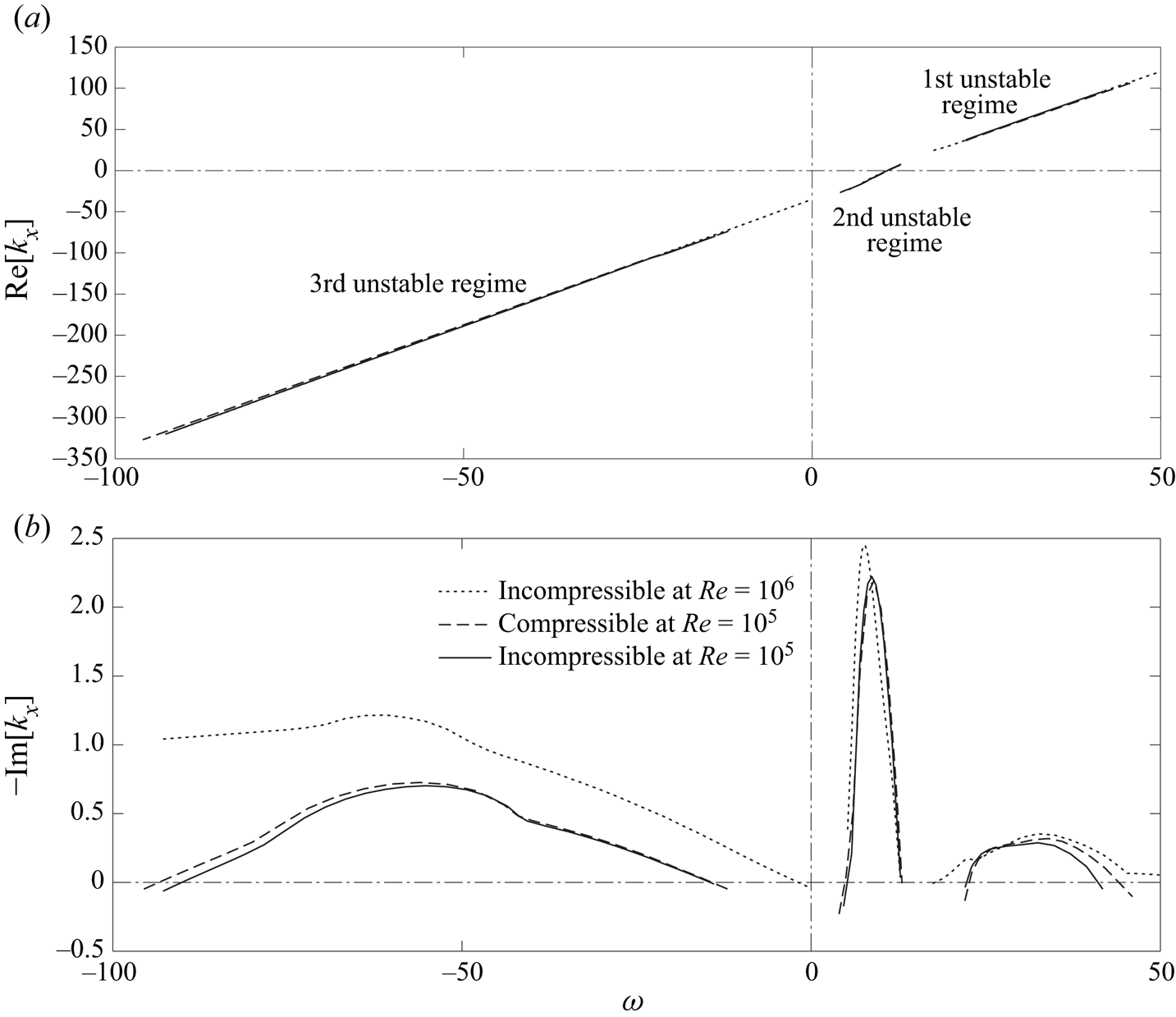
Figure 9 plots the dispersion relations solved as a spatial problem (4.4) near unstable ranges for the same condition as figure 5 (i.e.  $m = 22$ at the approach condition). Here, the figure compares three cases: the incompressible solutions at
 $Re = 10^5$ and
 $Re = 10^6$ and the compressible solution at
 $Re = 10^5$. The three solutions for the phase relation in figure 9(a) virtually overlap, indicating no impacts of the Reynolds number and the compressibility effect. The slope of the second unstable regime is slightly higher than the other two regimes. The growth rates in figure 9(b) somewhat depend on the Reynolds number; namely, the growth rates increase and the unstable ranges spread at the higher Reynolds number, particularly for counter-rotating modes (i.e. the third regime). The second mode always takes the highest growth rate, likely even at the Reynolds number of the real fan rig (
 $Re \approx 4 \times 10^6$).
Dispersion relations as a spatial problem of SDT for  $m = 22$ at
 $61.7\,\%$ RPM. (a) Axial wavenumber. (b) Growth rate.

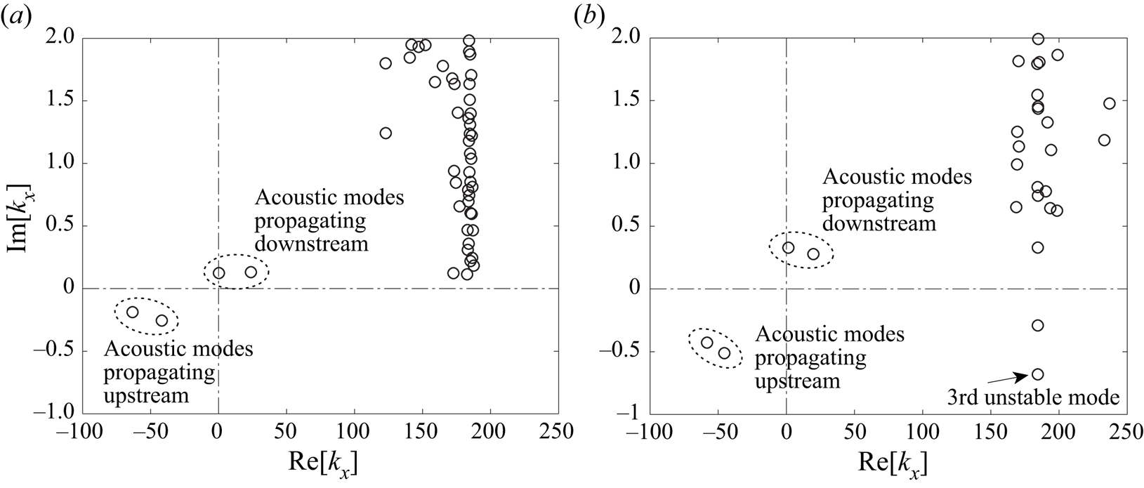
For  $m = 22$, acoustic modes start to branch out as a pair of highly decaying modes, one propagating downstream and the other upstream, somewhere at the non-dimensional angular frequencies of
 $\omega \gtrsim 60$ (
 $\approx 2.03 f_{{ BPF}}$) and
 $\omega \lesssim -40$ (
 $\approx -1.35 f_{{ BPF}}$) at the approach condition. These frequencies act as the threshold cut-on frequencies, which are skewed due to the swirl velocity, as explained in (4.8). As the frequency increases, the second pair of acoustic modes appears, and their decay rates become much less, say
 $\mbox {Im} [ k_x ] < 0.2$, at
 $\omega \gtrsim 72$ (
 $\approx 1.64 f_{{ BPF}}$) and
 $\omega \lesssim -49$ (
 $\approx -1.11 f_{{ BPF}}$). At these two frequencies, the eigenvalue distributions of the compressible analysis are plotted in figure 10 in the low
 $\mbox {Im} [ k_x ]$ range on the complex
 $k_x$ plane: as noted above, because the spatial problem is iteratively solved for a specific
 $k_x$ due to the nonlinear
 $k_x$ terms on the left-hand side of (4.4), values of
 $k_x$ are approximate except for the least-decaying acoustic mode in these plots.
Eigenvalue distribution of  $k_x$ at
 $61.7\,\%$ RPM (
 $Re = 10^5$); (a)
 $m = 22$ at
 $\omega = 72$, (b)
 $m = -22$ at
 $\omega = 49$.

In figure 10(a), there are no modes in the fourth quadrant (i.e. downstream-propagating growing mode) and in the second quadrant (i.e. upstream-propagating growing mode). In general, for co-rotating modes (i.e.  $m > 0$), the hydrodynamic mode is stable or very weakly unstable at such high frequencies; therefore, we expect that no acoustic modes excite hydrodynamic modes significantly at the same frequency and azimuthal mode. For
 $\omega < 0$, figure 10(b) plots
 $k_x$ by setting
 $m = -22$ so that
 $\mbox {Re} [ k_x ]$ takes the opposite sign relative to figure 9. We now find an unstable mode in the fourth quadrant. Namely, for counter-rotating modes (i.e.
 $m < 0$), acoustic modes in both directions can excite the hydrodynamic mode in the third regime, but magnitudes of counter-rotating hydrodynamic disturbances may be insignificant in the interstage.
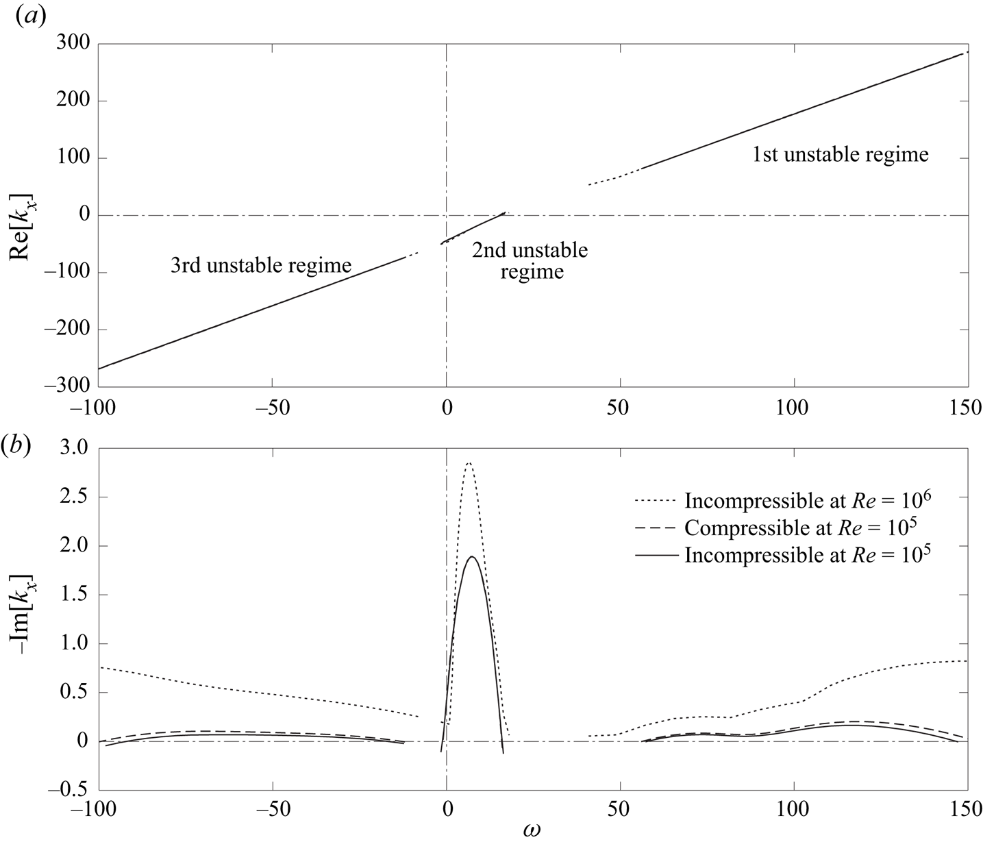
Figure 11(a) compares the dispersion relations at the cut-back condition. The phase relations for the three cases again overlap each other and retain the features found at the approach condition in figure 9(a). The comparison of the growth rates in figure 11(b) reveals that the Reynolds number has a significant impact, while the compressibility effect is still negligible at the cut-back condition. Compared with the approach condition, the first unstable regime spreads over a wider high-frequency range with a double-hump shape, but the peak growth rate at  $Re = 10^5$ becomes lower; in contrast, the other two unstable regimes tend to remain in similar frequency ranges. These trends are consistent with those derived by the temporal analysis shown in figures 5 and 6.
Dispersion relations as a spatial problem of SDT for  $m = 22$ at
 $87.5\,\%$ RPM. (a) Axial wavenumber. (b) Growth rate.

Such a large high-frequency shift of the first unstable regime can keep the hydrodynamic mode unstable beyond the cut-on frequency of the acoustic mode mentioned above. At the cut-back condition, the acoustic modes start to brunch out at  $\omega \gtrsim 65$ (
 $\approx 1.55 f_{{ BPF}}$) as a co-rotating mode of
 $m = 22$, and
 $\omega \lesssim -35$ (
 $\approx -0.84 f_{{ BPF}}$) as a counter-rotating mode of
 $m = -22$. Figure 12 similarly plots the complex
 $k_x$ distributions of both
 $m = \pm 22$ when the second acoustic modes appear on both directions. We confirm from figure 12(a) that the acoustic mode and the unstable hydrodynamic mode in the first regime now coexist with the same
 $m$ at the same
 $\omega$; however, this frequency (
 $\omega \gtrsim 77$) is much greater than the rotor speed (
 $m \varOmega \approx 41.9$). Therefore, it is unlikely that the amplification of hydrodynamic disturbances in the first unstable regime by acoustic modes has an appreciable impact on the rotor-related interaction noise.
Eigenvalue distribution of  $k_x$ at
 $87.5\,\%$ RPM (
 $Re = 10^5$); (a)
 $m = 22$ at
 $\omega = 77$, (b)
 $m = -22$ at
 $\omega = 43$.

At the take-off condition, we are unable to find unstable modes in the first and third regimes up to  $Re = 10^6$ (the first regime may exist beyond
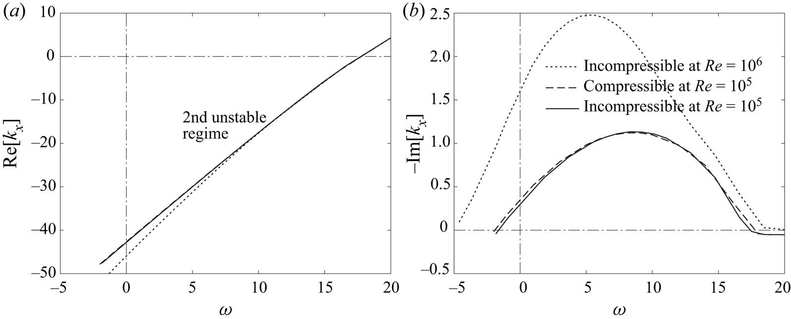
 $\omega > 300$, which is yet unresolvable with the current polynomial order). This is consistent with the observation in figure 7. This suggests that the interaction between the first and second unstable modes becomes weaker at higher engine speed. Accordingly, figure 13 plots the dispersion relations only in the second unstable regime. The growth rate is nearly doubled by increasing the Reynolds number by one order of magnitude. Across the three engine speeds, the peak growth rates of the second mode are found to be comparable at
 $Re = 10^6$, indicating the existence of the second unstable mode regardless of the engine speed (more precisely, the velocity profiles of these engine speeds). On the other hand, the compressibility effect remains to be negligible even at the take-off condition.
Dispersion relations as a spatial problem of SDT for  $m = 22$ at
 $100\,\%$ RPM. (a) Axial wavenumber. (b) Growth rate.

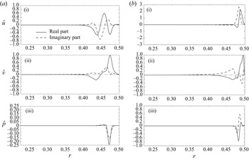
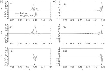
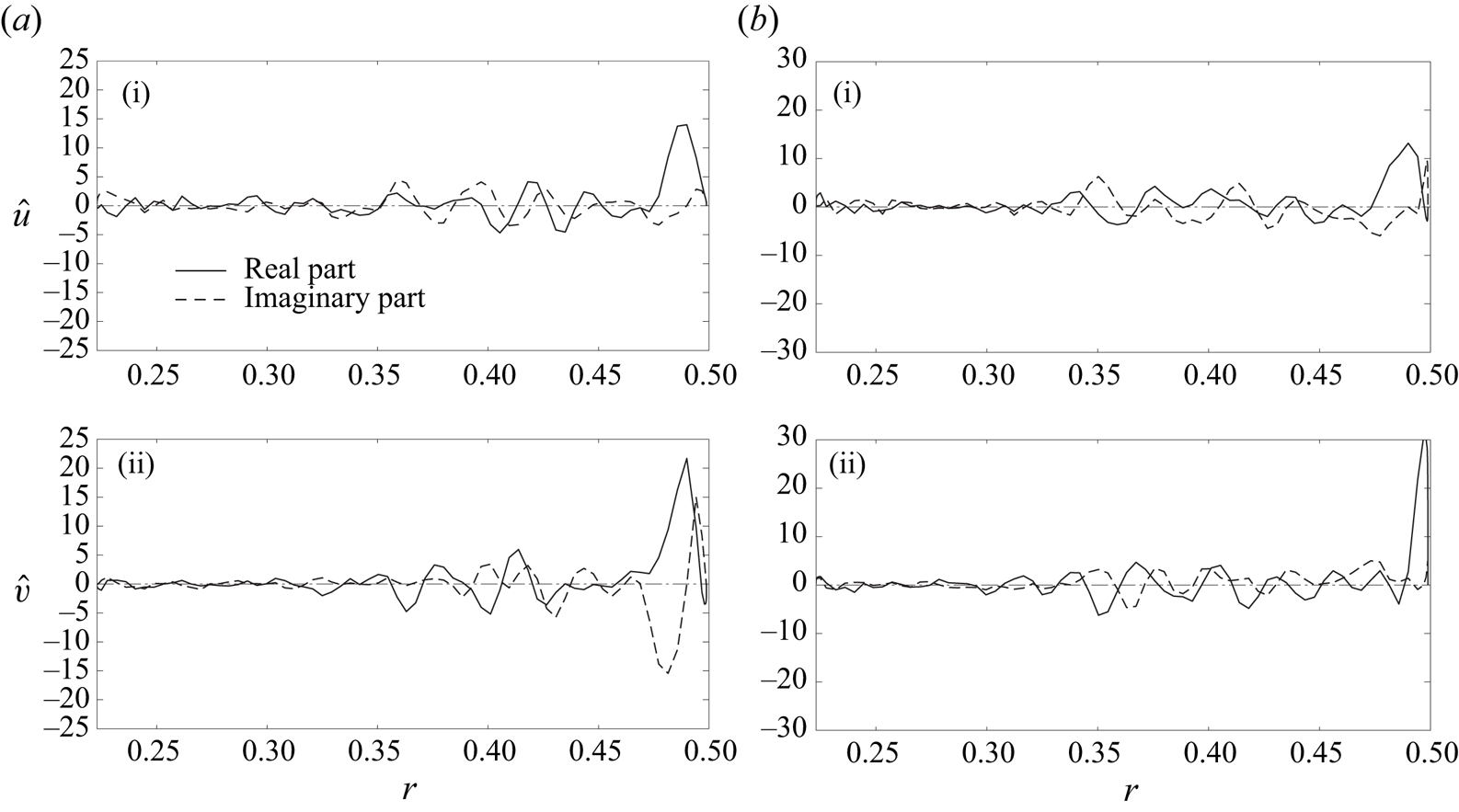
We now observe the eigenfunctions in the radial direction based on the compressible analysis. Figure 14 plots the eigenfunctions of the first and second unstable modes near the most unstable frequency in each regime at the approach condition. Both modes largely fluctuate near the outer wall; to be precise, the first mode forms a peak approximately above the outer-wall boundary layer, while the second mode resides inside of it. In contrast, figure 15, which similarly compares the eigenfunctions at the cut-back condition, reveals that the first mode is peaked away from the outer wall, while the second mode is still confined within the outer-wall boundary layer. These features are consistent with the radial profiles of turbulent kinetic energy in the interstage compared later in figure 18(b). This may also imply that the two modes can readily couple each other at  $61.7\,\%$ RPM, while they can hardly interact at
 $87.5\,\%$ RPM. If the interaction between the two modes contributes to the fan broadband noise, as hypothesized by Suzuki et al. (Reference Suzuki, Shur, Strelets and Travin2022), this noise-generation mechanism would be less important at high engine speeds. This may be one of the reasons why the contribution of the stripe patterns to the broadband noise is diminished in the azimuthal-mode map at higher speeds, as discussed in § 5.4 later, as well as from the mode-ring measurement by Premo & Joppa (Reference Premo and Joppa2002).
Eigenfunctions of the two unstable regimes for  $m = 22$ at
 $61.7\,\%$ RPM (
 $Re = 10^5$). (a) First mode (
 $\omega = 33$ in figure 9). (b) Second mode (
 $\omega = 9$). (i) Axial-velocity fluctuation. (ii) Azimuthal-velocity fluctuation. (iii) Pressure fluctuation.

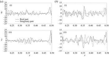
Eigenfunctions of the two unstable regimes for  $m = 22$ at
 $87.5\,\%$ RPM (
 $Re = 10^5$). (a) First mode (
 $\omega = 119$ in figure 11). (b) Second mode (
 $\omega = 7$). (i) Axial-velocity fluctuation. (ii) Azimuthal-velocity fluctuation. (iii) Pressure fluctuation.

4.4. Azimuthal-mode dependence
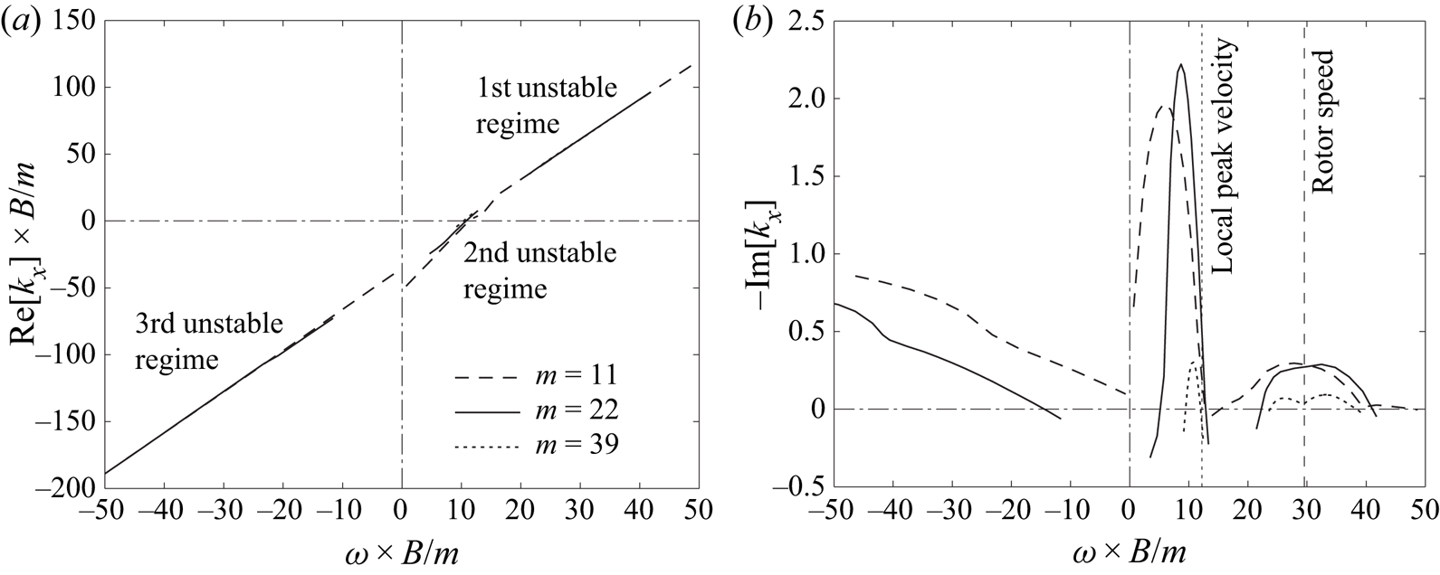
We observe the azimuthal-mode dependence, which clarifies the unstable range relevant to the rotor wakes. Figure 16 compares the dispersion relations of three different azimuthal modes near unstable frequency ranges at the approach condition by solving the incompressible problems at  $Re = 10^5$. As discussed in figure 8,
 $\omega$ and
 $k_x$ should reach the linear dependence on
 $m$ for a large asymptote of
 $m$ in (4.4); accordingly, figure 16 normalizes
 $\omega$ and
 $\mbox {Re} [ k_x ]$ with
 $m$ by taking the reference as the fan-blade count
 $B = 22$, except for
 $-\mbox {Im} [ k_x ]$. The phase relations collapse very well across all three regimes in figure 16(a). The unstable frequency ranges of the first and second regimes tend to align with the rotor speed and the local azimuthal velocity, respectively, in figure 16(b), but the peak growth rates depend on the azimuthal-mode number.
Dispersion relations of different azimuthal modes at  $61.7\,\%$ RPM (
 $Re = 10^5$). (a) Axial wavenumber. (b) Growth rate.

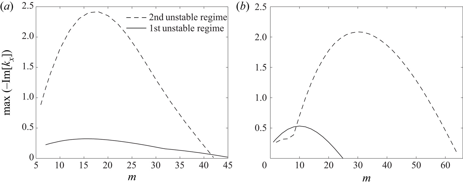
Figure 17 compares the peak growth rates of the first and second unstable regimes as a function of the azimuthal mode at  $Re = 10^5$. At the approach condition, the first and second regimes take the maximum values at similar azimuthal-mode numbers; accordingly, the first mode tends to amplify the wake disturbances in the vicinity of the fan-blade count. Moreover, the peak growth rate vanishes for
 $m \gtrsim 40$, and also other types of modes seem to take a higher peak growth rate for
 $m \lesssim 6$ (not shown) in both regimes. At the cut-back condition, in contrast, the unstable range of the first mode substantially shifts to the lower
 $m$ side, while the that of the second mode extends on the higher
 $m$ side. In fact, the unstable ranges of the second regime at both engine speeds coincide with the bundle of the stripe pattern in the azimuthal-decomposition map, shown later in figures 24, 29 and 30 (we discuss this point in §§ 5.3 and 5.4).
Peak growth rates as a function of the azimuthal mode at  $Re = 10^5$; (a)
 $61.7\,\%$ RPM, (b)
 $87.5\,\%$ RPM.

5. Analysis using the IDDES database
5.1. Post-processing of the IDDES database
To analyse the mode structures in the interstage and minimize artifacts in post-processing of the IDDES data for a limited time duration, the computational time-step was set to be  $\Delta t_{{ CFD}} \equiv 2 {\rm \pi}/ ( 2112 \varOmega )$, and an instantaneous velocity field was recorded in the rotating frame at every
 $16$ and
 $6$ time steps, i.e.
 $\Delta t_{{ DMD}} \equiv 2 {\rm \pi}/ ( 132 \varOmega )$ and
 $2 {\rm \pi}/ ( 352 \varOmega )$, at the approach and cut-back conditions, respectively. During two and one revolutions, a total of
 $N_t = 264$ and
 $352$ frames were recorded, respectively, while the azimuthal grid count in the interstage block was set to be
 $N_{\phi } = 792$. At the approach condition, the flow quantities in the rotating frame can then be projected onto the stationary frame by just clocking the mesh by six grids in the uniform grid region (in the upstream non-uniform grid region, they are interpolated into the same uniform grid), and also the same fan-blade position is repeated at every six recorded frames. At the cut-back condition, the flow quantities can be similarly projected on the stationary mesh by clocking
 $2.25$ grids with interpolation; consequently, the same fan-blade position is repeated at every
 $16$ recorded frames. In this process, the steady-wake component can be subtracted by averaging the flow quantities in the rotating frame, and the fluctuating components can be post-processed in the stationary frame to track their time evolution.
To extract coherent structures and compare them with the eigenfunctions from the linear stability analysis, the velocity fields were recorded on two planes, one plane being on a mid-axial station at  $x/D \approx 0.18$ and the other on a ‘quasi’-cylindrical surface (i.e. along iso-radial grid points) near the peak turbulent kinetic energy above the outer wall, as plotted in figure 18. On each plane, an approach equivalent to DMD formulated by Schmid (Reference Schmid2010) is applied to turbulent kinetic energy, which dictates hydrodynamic disturbances (details of the procedure are given in Suzuki et al. Reference Suzuki, Shur, Strelets and Travin2022): after velocity fluctuations are azimuthally decomposed up to
 $m = 44$ modes (i.e. twice the fan-blade count) on each plane, snapshot proper orthogonal decomposition (POD) modes (Sirovich Reference Sirovich1987) are obtained by optimizing the turbulent kinetic energy, and the time histories of the POD coefficients are then computed. Subsequently, the linear evolution among limited POD coefficients is calculated using a generalized-inverse technique (Perret, Collin & Delville Reference Perret, Collin and Delville2006). If the linear transfer matrix is eigen-decomposed, the sets of the eigenvalue and eigenvector can be regarded as DMD modes except that higher-order POD modes, which are less coherent, have been excluded.
Surfaces on which DMD modes are extracted. (a) Mid-station plane and quasi-cylindrical surface. (b) Position of the quasi-cylindrical surface relative to turbulent kinetic energy at  $x \approx 0.18$.

In addition to the velocity fields, pressure fields on the interstage outer wall are also post-processed mainly to analyse acoustic modes. The wall-pressure fluctuations in the stationary frame are obtained by similarly clocking and interpolating the azimuthal grids, and those at  $x/D \approx 0.18$ are azimuthally decomposed using the full
 $N_{\phi } = 792$ grids over the frequencies. In addition, the snapshot POD analysis is applied to extract coherent modes dominating the wall pressure, and the time histories of the leading POD-mode coefficients are Fourier transformed to calculate their frequency spectra.
5.2. The DMD modes extracted from velocity fields on two planes
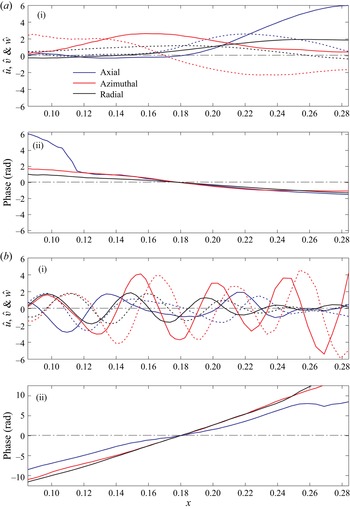
We first observe mode structures on the cylindrical surface near the outer wall by taking  $m = 23$ at the approach condition, which is considered to be the peak of the azimuthal-mode power in figure 31(a) shown later. Figure 19 exhibits the velocity fluctuations of typical DMD modes that represent eigenfunctions in the first and second unstable regimes. In this study, we count the order of DMD modes so that the first mode contains the greatest turbulent kinetic energy. The first unstable mode, which is the fifth DMD mode in this case, changes the phase rapidly due to a high axial wavenumber. In contrast, the second unstable mode, which is the second DMD mode in this case, appears to grow monotonically with a very small negative wavenumber. For
 $m = 23$, the first four DMD modes all belong to the second unstable regime, and many higher modes depict wavepacket structures, growing and decaying weakly in the axial direction, relevant to the first unstable regime, as shown in figure 20(b i) below.
Typical DMD modes near the wall for  $m = 23$ at
 $61.7\,\%$ RPM. Colour schemes are common to all plots. (a) Second DMD mode representing the second unstable regime. (b) Fifth DMD mode representing the first unstable regime. (i) Amplitude. Line patterns are common to all components. (ii) Phase. Negative slope denotes an upstream-propagating mode and vice versa.

Typical DMD modes near the wall for  $m = 18$ at
 $87.5\,\%$ RPM. Colour schemes and line patterns are the same as figure 19. (a) First DMD mode representing the second unstable regime. (b) Third DMD mode representing the first unstable regime. (i) Amplitude. (ii) Phase.

Likewise, figure 20 shows typical DMD modes at the cut-back condition. Here, we take  $m = 18$, which is a local peak in the azimuthally decomposed PWL contour shown later in figure 31(b). The first DMD mode seems to be close to an eigenfunction in the second unstable regime (or a slightly higher frequency/wavenumber). The third DMD mode represents the characteristics of the first unstable regime; in particular, this DMD mode indicates a clear wavepacket structure. Compared with the approach condition, the number of DMD modes in the first regime becomes more dominant than that in the second regime for the cut-back condition, which can be confirmed in figure 21 below.
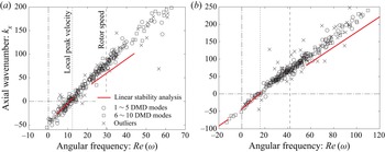
Dispersion relations of the first  $10$ DMD modes overlaid from
 $m = 14$ to
 $41$.
 $\omega$ and
 $k_x$ are multiplied by
 $\times B/m$ (i.e. normalized to
 $m = 22$); (a)
 $61.7\,\%$ RPM, (b)
 $87.5\,\%$ RPM.

Figure 21 overlays the dispersion relations of the first ten DMD modes for each azimuthal mode from  $m = 14$ to
 $41$ extracted from the IDDES at the approach and cut-back conditions. Here, we take the frequency directly from the DMD analysis and calculate the axial wavenumber from the slope of the phase averaged among the three velocity components at
 $x/D = 0.18$. If there is either a discontinuity in the phase over the axial extent or a discrepancy between the three phase slopes, such a DMD mode is declared as an outlier. To also compare them with the dispersion relation predicted by the compressible linear stability analysis in figures 9 and 11,
 $\omega$ and
 $k_x$ are scaled by multiplying them by
 $B/m$. For reference, the local peak of the azimuthal velocity and the rotor speed are also drawn.
Figure 21 reveals that the IDDES data collapse very well at both approach and cut-back conditions. The linear stability analysis predicts the extracted dispersion relations generally well except for outliers, although it slightly under-estimates the wavenumber for the first unstable regime for an unknown reason. For both engine speeds, we can find one cluster in the second unstable regime (i.e. along the straight line near the origin), and another cluster near the rotor speed, which represents modes convecting with the rotor wakes. In particular, the separation between the first and second regimes is discernible in figure 21(a). In figure 21(b), in contrast, the biggest cluster appears between the first and second regimes. We should recall that the eigenfunction for the first regime forms a peak away from the outer wall at  $87.5\,\%$ RPM, as plotted in figure 15(a); hence, the velocity fluctuations on this cylindrical surface may not be exactly representative of the first unstable mode. Nonetheless, figures 20(b) and 21(b) suggest that the first unstable mode carries coherent structures in the rotor wakes without decaying the amplitude.
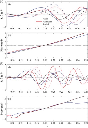
Next, we observe the radial dependence of the coherent structures. Figure 22 plots the velocity fluctuations of typical leading-order DMD modes for  $m = 23$ at the approach condition. In this example, the second and fourth DMD modes take the frequencies corresponding to the first and second unstable regimes, respectively. In both DMD modes, we find large fluctuations near the outer wall, and the difference in the peak radial position is not as clear as that of the eigenfunctions between the first and second modes plotted in figure 14. Since coherent structures between the two unstable regimes seem to interact in the outer-wall boundary layer, separation between them on the same station might be difficult in the post-processing.
Typical DMD modes on the mid-station plane at  $61.7\,\%$ RPM (
 $m = 23$). (a) Second DMD mode (
 $\omega = 31.1$). (b) Fourth DMD mode (
 $\omega = 0.11$). (i) Axial-velocity fluctuation. (ii) Azimuthal-velocity fluctuation.

At the cut-back condition, the coherence becomes weaker than the approach condition; namely the turbulent kinetic energy contained in the leading-order POD modes becomes less, and this makes the extraction of coherent modes challenging. Figure 23 similarly plots the radial profiles of typical DMD modes for  $m = 18$ at the cut-back condition. The second DMD mode takes a frequency in the second unstable regime, while the frequency of the third DMD mode is close to the first unstable regime. The latter mode shows relatively large fluctuations in the mid span, which is consistent with the linear stability analysis in figure 15, but also near the outer wall. In many fast co-rotating DMD modes (i.e. large
 $\omega > 0$), we find similar structures (not shown). In contrast, the former mode forms a peak clearly in the outer-wall boundary layer, as predicted by the linear stability analysis. The number of DMD modes found in the second unstable regime is relatively small at the cut-back condition, while the DMD modes with large fluctuations in the mid span are rather dominant. In fact, figure 18(b) supports this observation.
Typical DMD modes on the mid-station plane at  $87.5\,\%$ RPM (
 $m = 18$). (a) Second DMD mode (
 $\omega = 27.1$). (b) Third DMD mode (
 $\omega = 78.5$). (i) Axial-velocity fluctuation. (ii) Azimuthal-velocity fluctuation.

5.3. Pressure fluctuations on the outer wall
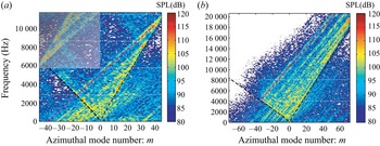
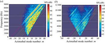
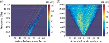
By azimuthally decomposing the wall-pressure fluctuations at the middle of the interstage, we can directly observe the rotor–stator and rotor-related interactions and the cut-on boundaries of the duct acoustic modes. Unlike the inlet/exhaust mode analysis, it is non-trivial to prescribe duct acoustic modes for the mode-extraction method (Ovenden & Rienstra Reference Ovenden and Rienstra2004) due to the swirl velocity, as explained in § 4.3. Thus, we only consider the azimuthal-mode decomposition along a single ring at  $x/D \approx 0.18$, and figure 24 displays the decomposed sound pressure level (SPL) as a function of
 $m$ over the frequencies at the approach and cut-back conditions. The shaded area on the top left corner of figure 24(a) indicates the region in which aliased positive
 $m$ modes are contaminated due to a low sampling rate. Although non-acoustic components are included on the wall-pressure fluctuations, a V-shape cut-on region can be clearly seen for both conditions. Here, the skewed cut-on boundaries are very well predicted by (4.8) by setting
 $\chi = 0.35$. High SPL can be observed along these boundaries, especially on the co-rotating side (i.e.
 $m > 0$), which can also be found in the experiment (Premo & Joppa Reference Premo and Joppa2002). Some SPL can be discerned along the boundary on the counter-rotating side, but these modes are decaying once the cut-on boundaries become symmetric in the inlet or the exhaust.
Azimuthal-mode decomposition of the wall SPL in the interstage. Horizontal white dotted lines denote the BPF and the harmonics. Skewed V-shape black dashed lines represent the cut-on boundaries predicted by (4.8). Inclined magenta dashed line denotes the rotor speed interacting with the threshold  $m_0$; (a)
 $61.7\,\%$ RPM (
 $m_0 = -39$), (b)
 $87.5\,\%$ RPM (
 $m_0 = -57$).

Importantly, fluctuations are noticeable even outside the cut-on zone along multiple lines from the left bottom to the right top with the slope representing the rotor speed. When a disturbance of the azimuthal mode  $n_B$ spinning at the rotor speed
 $\varOmega$ is interacting with a quasi-stationary object of the azimuthal mode
 $m_0$ moving at
 $\varOmega _0$ (
 $\approx 0$), it creates the azimuthal mode of
 $m = n_B + m_0$; hence, the mode line appears in figure 24 along
 \begin{equation} f\, ({\rm Hz}) = \frac{n_B \varOmega - m_0 \varOmega_0}{2 {\rm \pi}} = \frac{\varOmega}{2 {\rm \pi}} \left( m - m_0 \right) - \frac{\varOmega_0}{2 {\rm \pi}} m_0 \approx \frac{\varOmega}{2 {\rm \pi}} \left( m - m_0 \right) . \end{equation}
If multiple quasi-stationary structures of  $m_0$ are moving with different speeds of
 $\varOmega _0$, the second term
 $\varOmega _0 m_0 / ( 2 {\rm \pi})$ becomes obscure, and lines only along the rotor speed remain to be noticeable. Namely, figure 24 suggests that multiple quasi-stationary structures are interacting with broadband motions spinning at the rotor speed. The threshold azimuthal-mode count
 $m_0$ drawn by the magenta dashed line approximately corresponds to the cut-off wavenumber of the VSTG (
 $| m_0 | \lesssim 39$ and
 $\lesssim 57$ at the approach and the cut-back conditions, respectively). When the
 $n-1$th harmonic of the fan-blade count
 $B$ (i.e.
 $n_B = nB$) interacts with the
 $k_n-1$th harmonic of the OGV count
 $V_n$ (i.e.
 $m_0 = k_n V_n$ and
 $\varOmega _0 = 0$), it yields the Tyler & Sofrin (Reference Tyler and Sofrin1962) relation, generating the
 $nB + k_n V_n$ azimuthal mode at the frequency
 $n B \varOmega / ( 2 {\rm \pi})$, where the BPF is given by
 $f_{{ BPF}} \equiv {B \varOmega }/{( 2 {\rm \pi})}$.
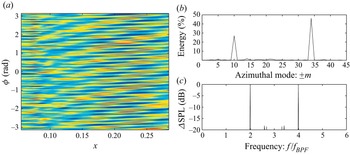
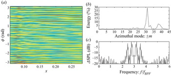
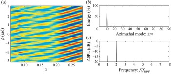
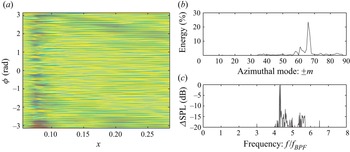
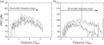
To extract coherent modes among the wall-pressure fluctuations, the snapshot POD method (Sirovich Reference Sirovich1987) is applied in the physical domain. On the  $x - \phi$ domain in the stationary frame, snapshot POD modes on the outer wall are unwrapped, and a few representative modes are displayed from figures 25 to 28. The azimuthal-mode distribution averaged over
 $x$ is also plotted for each POD mode. Moreover, time histories of the POD-mode coefficients are calculated, and a frequency spectrum of each POD mode is given as well. Although the sampling rate was low at the approach condition, it is still meaningful to show it beyond the Nyquist frequency; thus, the spectrum including both sides (i.e. symmetric spectrum across
 $3f_{{ BPF}}$) being depicted in figures 25(c) and 26(c). At the approach condition, the first POD mode captures the rotor–stator interaction tones; namely, 2BPF with
 $m = -10$ and 4BPF with
 $m = 34$. The second POD mode (not shown) is very similar to the first POD mode. The fourth (and sixth, not shown) POD mode has a peak around
 $2.8 f_{{ BPF}}$ in the broadband with the azimuthal peak of
 $m = 31$. We can find the corresponding spot along a stripe of the broadband noise in figure 24(a), suggesting that the aforementioned stripes have strong coherency.
First snapshot POD mode of the wall-pressure fluctuation at  $61.7\,\%$ RPM. (a) Unwrapped pressure contour. (b) Azimuthal-mode distribution averaged over
 $x$. (c) Frequency spectrum of the POD-mode coefficient.

Fourth snapshot POD mode of the wall-pressure fluctuation at  $61.7\,\%$ RPM. Same layout as figure 25.

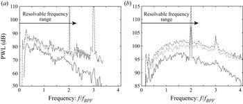
Third snapshot POD mode of the wall-pressure fluctuation at  $87.5\,\%$ RPM. (a) Unwrapped pressure contour. (b) Azimuthal-mode distribution averaged over
 $x$. (c) Frequency spectrum of the POD-mode coefficient.

Fifth snapshot POD mode of the wall-pressure fluctuation at  $87.5\,\%$ RPM. Same layout as figure 27.

Likewise, figures 27 and 28 show representative snapshot POD modes at the cut-back condition. Unlike the approach condition, the sampling rate was high enough so that each figure (c) plots one side of the spectrum. The third (and fourth, not shown) POD mode captures the 2BPF tone with  $m = -10$ in figure 27 (although not shown, the first two POD modes take the BPF tone with
 $m = -32$). Compared with the approach condition, these tone intensities are clearly higher downstream, indicating the conventional rotor–stator interaction. In contrast, the fifth (and sixth, not shown) POD mode represents broadband noise around
 $4.2 f_{{BPF}}$ with
 $m \approx 66$ in figure 28. This peak appears as a strong SPL spot in figure 24(b) along a stripe. We should remark that when the POD mode is found close to the cut-on boundary, i.e. non-dimensional wavenumber of
 $k_x \ll 1$ so that the unwrapped pressure contour depicts almost horizontal stripes regardless of tones or broadband noise. In this sense, the wavenumber structures of these acoustic modes are somewhat similar to the aforementioned second unstable modes. Yet, because of the difference in the frequency range, these POD modes can be confirmed as the acoustic modes (note that the pressure field in the aforementioned quasi-cylindrical surface is dominated by these acoustic modes).
The results above suggest that the wall-pressure fluctuations in the interstage are largely influenced by the rotor–stator interaction tones satisfying the Tyler–Sofrin relation (Tyler & Sofrin Reference Tyler and Sofrin1962) as well as the interaction between disturbances moving with the rotor speed and those generated downstream of the rotor (likely spinning slowly). The latter disturbances may be governed by the instability in the second regime, which is found to dominate coherent hydrodynamic structures near the outer wall. Within the skewed cut-on boundaries of the interstage flow, strong coherent acoustic modes can be found in the broadband noise as a result of such an interaction. Although it has been revealed by Golubev & Atassi (Reference Golubev and Atassi1998) that acoustic modes possess a vortical component and hydrodynamic modes possess pressure fluctuations under swirl velocity, which has been confirmed in figures 10 and 12, such couplings do not seem to be the dominant interaction mechanism. These broadband noise generation seems to be rather caused by the nonlinear product of two different types of non-acoustic disturbances.
5.4. Contribution to fan broadband noise
Finally, we relate the stripe patterns with the sound properties radiating from the inlet and the exhaust. Figures 29 and 30 display the azimuthal-mode decomposition of the inlet/exhaust duct acoustic-mode PWL at the approach and cut-back conditions, respectively. Suzuki et al. (Reference Suzuki, Spalart, Shur, Strelets and Travin2019) described the procedure of the mode-extraction method (Ovenden & Rienstra Reference Ovenden and Rienstra2004) specifically tailored for the fan-noise simulations. In general, these IDDES results are consistent with the azimuthal-mode decomposition of the wall-pressure fluctuations measured by Premo & Joppa (Reference Premo and Joppa2002). A particular interest here is the stripe patterns drawn by the inclined lines: as explained in § 5.3, the slope of these lines represents the rotor speed, and the azimuthal-mode numbers at the root of the lines (i.e. at  $0$ Hz) indicate the mode counts of the quasi-stationary structures. The magenta line corresponds to the threshold wavenumber of the VSTG, introduced in § 3 and figure 24 (
 $| m_0 | \le 39$ and
 $\le 57$ at the approach and cut-back conditions, respectively). The yellow lines represent the local azimuthal peaks of the inlet/exhaust PWL spectra identified in figure 31 below.


Azimuthal-mode decomposition of the duct-mode PWL at  $87.5\,\%$ RPM. (a) Inlet. (b) Exhaust.

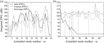
Integrated PWL along the inclined lines on the azimuthal PWL contours in the inlet and the exhaust (scaled by dB on the left axis). Integrated SPL of the azimuthal SPL contours in the interstage is also plotted (offset by  $25$ dB); (a)
 $61.7\,\%$ RPM, (b)
 $87.5\,\%$ RPM.

By integrating the PWL along these inclined lines, the radiating sound power can be calculated as a function of the azimuthal-mode number associated with the potentially stationary structures (i.e.  $m$ values at
 $0$ Hz). In figure 31, such PWLs are compared between the inlet and the exhaust together with the SPL on the interstage wall similarly integrated along the inclined lines in figure 24 (the interstage SPL is offset by
 $25$ dB). Here, similar azimuthal-mode patterns are depicted between the inlet and the exhaust as well as the interstage, particularly at the approach condition. At the cut-back condition, the PWL is rapidly decreased toward greater
 $-m$ in the inlet due to the transonic rotor speed, while the PWL is spread over a wide azimuthal-mode range in the exhaust and the interstage. More importantly, many common peaks, indicated by the vertical dotted lines, can be identified among the three regions, but they are smeared in the inlet and the exhaust at the cut-back condition. This suggests an existence of a broadband noise-generation mechanism at both approach and cut-back conditions, and it contributes commonly to the inlet and exhaust PWL spectra. This noise-generation mechanism appears to play a major role in the fan broadband noise at the approach condition but the relative importance becomes less at the cut-back condition, particularly in the inlet. By comparing figures 29(a) with 30(a), it is clear that the noise directly related to the transonically spinning rotor, which is distributed along the cut-on line on the co-rotating side, is significantly increased at the cut-back condition.
To crudely assess the magnitude of the PWL contained in the stripes of the IDDES results, the following steps are taken (for a detailed procedure, refer to Suzuki et al. Reference Suzuki, Shur, Strelets and Travin2022, particularly figure 10): first, the azimuthally decomposed PWL along the inclined lines in figure 29 or 30 is filtered using the five-point smoothing (Savitzky & Golay Reference Savitzky and Golay1964) in frequency. Second, troughs are identified in the azimuthal distribution of the PWL within the azimuthal bundle confined by the aforementioned threshold  $m_0$ of the VSTG. By linearly connecting the troughs together with the PWL distribution outside the azimuthal range, the background PWL is then defined, and the logarithmic difference between the total and the background PWLs is eventually treated as the segregated PWL in the stripes. Thus, the extra contribution in the stripes is graphically extracted.
Figure 32 plots the breakdown of the spectra from the mode extraction at the approach condition by summing the background and segregated PWL over the azimuthal modes. Fluctuations in the PWL spectra are somewhat high even in the total spectra due to a narrow bandwidth to compare with the test spectra in the series of this study; however, these figures capture the trends of the PWL in the stripes. In the inlet, the segregated spectrum in the stripes appears to have comparable PWL to the rest of the background PWL, which should characterize the conventional rotor–stator interaction noise. In the exhaust, the PWL in the stripes steeply declines at higher frequencies, partially because of the greater total PWL in the exhaust at higher frequencies. As visually observed, the contribution from the stripes seems to be more relevant to the inlet broadband noise.
Breakdown of the PWL spectra at  $61.7\,\%$ RPM assessed by the steps given by Suzuki et al. (Reference Suzuki, Shur, Strelets and Travin2022). Line patterns:
 $-~-~-$, total;
 $\cdot \cdot \cdot \cdot \cdot$, background; —–, segregated. (a) Inlet. (b) Exhaust.

Likewise, figure 33 plots the breakdown at the cut-back condition. The contribution from the segregated spectrum relative to the total PWL spreads over wide frequencies, but it is typically lower by  $6$ dB or more; hence the relative contribution of this noise-generation mechanism seems to be weaker at
 $87.5\,\%$ RPM than
 $61.7\,\%$ RPM, which can be observed by comparing figures 29 and 30. Although the procedure of this breakdown is nothing but a pattern recognition, these results suggest that such a noise-generation mechanism appreciably contributes to the fan broadband noise at the approach condition, but becomes less important at the cut-back condition.
Breakdown of the PWL spectra at  $87.5\,\%$ RPM assessed by the steps given by Suzuki et al. (Reference Suzuki, Shur, Strelets and Travin2022). Line patterns are the same as figure 32. (a) Inlet. (b) Exhaust.

6. Conclusions
Unstable modes in an interstage flow between the rotor and the stator in turbomachinery have been analysed, and their impact on the fan noise has been investigated. By viewing the interstage flow as Taylor–Couette flow with the axial component or as spiral Poiseuille flow, compressible and incompressible linear stability analyses have been performed with velocity profiles taken from the IDDES simulation of a high-speed turbofan rig, called SDT. From this CFD database, which solved an entire rotor–stator system with a hard-wall nacelle, coherent hydrodynamic modes have been successfully extracted in the interstage using an approach equivalent to DMD, and these DMD modes have been compared with eigenfunctions of the linear stability analysis. The outer-wall pressure fluctuations have also been Fourier decomposed in the interstage, and the relation between these hydrodynamic instabilities and duct acoustic modes has been explored. Eventually, possible impacts of these instabilities on the fan broadband noise associated with the rotor-related interaction have been considered.
The viscous linear stability analysis has included the compressibility effect and assumed an infinitely extended annulus by ignoring the eddy viscosity and the steady-wake pattern. A spectral method using the Chebyshev polynomials can solve a temporal or spatial eigenvalue problem up to approximately  $Re \approx 3 \times 10^5$. The analysis has revealed three distinct unstable regimes: the first mode can excite disturbances above the outer-wall boundary layer over a wide frequency range including the rotor speed. This mode has higher axial wavenumbers and relatively low growth rates at low Reynolds numbers. The growth rate diminishes downstream with increasing thickness of the azimuthal-velocity peak, forming wavepacket-like structures above the outer-wall boundary layer. The second mode evolves approximately with the local azimuthal velocity and stays closer to the outer wall. The growth rate depends less on the Reynolds number and the velocity profile variation. This mode fluctuates at lower frequencies with much smaller axial wavenumbers, potentially acting like quasi-stationary structures over the outer wall. The third mode rotates in the opposite direction (i.e. a counter-rotating mode) and possesses characteristics similar to the first unstable regime. This study confirmed that the compressibility effect is negligible even at the take-off condition; however, the resultant velocity profile has a significant impact so that only the second unstable regime survives at the take-off condition.
By post-processing the IDDES database, the analysis equivalent to DMD supports the existence of these instabilities in the interstage even at  $Re \approx 4 \times 10^6$: typical DMD modes capture the dispersion relations and the radial shapes of the eigenfunctions predicted by the linear stability analysis in spite of its idealizations. Thus, these unstable modes dictate coherent structures of the velocity fluctuations in the interstage. At the approach condition, the first and second unstable modes can strongly interact near the outer wall. At the cut-back condition, however, fluctuations associated with the first unstable regime seem to migrate away from the outer wall, so that the interaction between the first and second modes may become weaker. Decomposition of the outer-wall-pressure fluctuations has demonstrated that duct acoustic modes characterized in a uniform flow with rigid-body rotation govern the pressure field in the interstage, and the azimuthally decomposed SPL contours depict a stripe pattern similarly to the inlet and exhaust PWL contours. We can relate primary POD modes of the interstage pressure fluctuations not only to the Tyler–Sofrin tones but also to high SPL spots along the stripes on these contours.
The series of the analyses in this study implies the impact of the interstage instabilities on the fan broadband noise as follows: from the frequency and azimuthal-mode ranges of the first unstable regime and the DMD of the IDDES data, it becomes clear that the first unstable mode enhances coherent structures in the rotor wakes. The wall-pressure decomposition in the interstage has revealed that these coherent structures moving with the rotor wakes nonlinearly interact with quasi-stationary structures and generate duct acoustic modes, causing a stripe pattern in the fan broadband noise at both approach and cut-back conditions. A candidate of such a structure is the second unstable mode near the outer wall, which has been confirmed through the DMD analysis. This interaction noise seems to be radiated to both inlet and exhaust with similar azimuthal-mode distributions. This mechanism is different from the fan broadband noise sources considered in the past, and may occupy a good fraction of it, particularly at low speeds. At higher engine speeds, however, the relative importance of this noise source decreases because the broadband noise originated from the fan blades becomes stronger beyond the cut-back condition.
Acknowledgments
The author would like to express deep appreciation to Professor M.L. Shur, Professor M.K. Strelets and Professor A.K. Travin, who provided the IDDES database in the past and agreed to use it for this study. The author would also like to thank Professor S.K. Lele for advice on a spectral method and Professor Y. Murai for an insight into the Taylor–Couette instability. The author also greatly appreciates Dr E. Envia, who kindly shared the SDT database, Dr Gonzalez-Martino and Dr D. Casalino, who also shared their CFD result, as well as Dr P.R. Spalart, who provided critical comments.
Declaration of interests
The author reports no conflict of interest.
Appendix. Comparison of IDDES results with SDT test data
In figure 34, the phase-locked axial- and azimuthal-velocity components in the interstage at the cut-back condition are compared between the IDDES result and the LDV measurement by G. Podboy. The time-averaged velocity field is very well predicted by the IDDES, as observed at the approach and take-off conditions in Shur et al. (Reference Shur, Strelets, Travin, Spalart and Suzuki2018c). The velocity fluctuations are also captured well, except for the thin outer-wall region. A high root-mean-square (r.m.s.) spot, which probably represents a tip vortex from a fan blade, is clearly found in the LDV result, while it is less emphasized in the IDDES partly because the wall boundary layers were solved as the Reynolds-averaged Navier–Stokes (RANS) mode. Nonetheless, two separated high fluctuation regions, one near the outer wall and the other in the middle of the span, are identified in the IDDES, which can also be confirmed in figure 18(b).
Comparison of the phase-locked velocity components at  $87.5\,\%$ RPM. Time-averaged and r.m.s. axial and azimuthal components at
 $x \approx 0.18$ are displayed. (a) IDDES. (b) LDV (figure is taken from Gonzalez-Martino & Casalino (Reference Gonzalez-Martino and Casalino2018) with permission).

The PWL spectra calculated from the IDDES are compared with the SDT data taken by a traverse microphone by Woodward et al. (Reference Woodward, Hughes, Jeracki and Miller2002) at the approach and cut-back conditions in figures 35 and 36, respectively. The PWL of the IDDES was obtained in two ways: one was to integrate the SPL computed by the Ffowcs-Williams & Hawkings technique (Ffowcs Williams & Hawkings Reference Ffowcs Williams and Hawkings1969) from  $0^{\circ }$ to
 $180^{\circ }$ along the traverse-microphone line. The control surfaces were designed to separately enclose the inlet and the exhaust including the fan-stream jet (refer to figure 3(b) in Suzuki et al. Reference Suzuki, Spalart, Shur, Strelets and Travin2019). The other was to sum all cut-on duct acoustic modes, which were extracted with the method developed by Ovenden & Rienstra (Reference Ovenden and Rienstra2004) by fitting pressure and axial-velocity fluctuations on four planes. Correspondingly, the spectra of the complete rotor–stator configuration and the spectra associated only with the stator are plotted from the SDT experimental data.
Comparison of PWL spectra between the IDDES and the SDT data at  $61.7\,\%$ RPM. (a) Inlet. (b) Exhaust.

Comparison of PWL spectra between the IDDES and the SDT data at  $87.5\,\%$ RPM. Line patterns are the same as figure 35. (a) Inlet. (b) Exhaust.

At the approach condition, very good agreement is found in both inlet and exhaust spectra up to the resolvable frequency ranges in figure 35. The low-frequency noise of the SDT data in the exhaust may be caused by the interaction of the fan-stream jet with the downstream strut, which was not modelled in the CFD. At the cut-back condition, in contrast, the broadband level is significantly under-predicted by the IDDES, particularly in the inlet in figure 36(a) (here, the assumed averaged Mach number in the inlet needs to be additionally increased by  $10\,\%$ for the mode-extraction method to make the rotor-locked tones cut-on). In Suzuki et al. (Reference Suzuki, Spalart, Shur, Strelets and Travin2019), very similar trends were reported at the take-off condition.
It should be recalled that unsteady turbulence was not resolved in the boundary layers on the inlet walls as well as on the fan blades, and the broadband noise sources associated with these components were not included in the IDDES. From these results, it may be deduced that the broadband noise mechanisms at low-speed conditions are captured by the rotor–stator interaction, while at high speeds, additional mechanisms, such as the interaction between the wall boundary layer and the rotor tip as well as the interaction between the boundary layer over the blade surface and the fan trailing edge, are probably more important. It should also be noted that the mechanical engine speed at the cut-back condition in the test appears to be higher than the reported/corrected speed ( $11\,074$ RPM) by approximately
 $1.6\,\%$ based on the BPF tones. This might substantially broaden the cut-on region such that the BPF is clearly cut-on in the SDT, while the BPF tone of the IDDES is buried underneath the broadband in figure 36(b). In fact, Suzuki et al. (Reference Suzuki, Spalart, Shur, Strelets and Travin2018) demonstrated that the IDDES predicts the cut-on tone PWL relatively well even at the take-off condition.