

Introduction
Usually soils exhibit important spatial variability because of many physical, biological and chemical processess acting simultaneously with different intensities. Consequently, uniform management of fields does not take into account the spatial variability, not the most effective management strategy. Identification of homogeneous regions, with similar characteristics, such as texture, topography, nutrient levels, etc., within the field is the first step to implement site-specific management, but this is not an easy task due to the complex interactions of all factors that could affect crop yield. However, it is known that the physical and chemical properties of the soil are one of the factors most affecting crop yields (e.g. Ortega et al., Reference Ortega, Westfall, Gangloff and Peterson1999), so they must be taken into account to delimit homogeneous zones. These are referred to as management zones (MZ), that is, subfields of similar production potential.
Significant research effort has been directed towards evaluating different techniques to define stratified within-field MZ. These approaches, with varying degrees of success, include, for instance, electrical conductivity sensors (Johnson et al., Reference Johnson, Mortensen, Wienhold, Shanahan and Doran2003), yield maps (Diker et al., Reference Diker, Heermann and Brodahl2004), and the consideration of farmer´s knowledge (Fleming et al., Reference Fleming, Heermann and Westfall2004). During recent years, different algorithms have been used to integrate the main variables: the utilisation of the coefficient of variation of each data layer (Ortega and Santibañez, Reference Ortega and Santibáñez2007), the use of a cluster procedure using the fuzzy c-means methods (e.g. Moral et al., Reference Moral, Terrón and Marques da Silva2010), or the use of principal component analysis, alone or in combination with the cluster method (e.g. Morari et al., Reference Morari, Castrignanò and Pagliarin2009).
A first attempt to properly integrate the data from some soil variables based on the use of the Rasch model (Rasch, Reference Rasch1980) was proposed by Moral et al. (Reference Moral, Terrón and Rebollo2011). Despite this probabilistic approach having been used successfully in some environmental applications (e.g. Moral et al., Reference Moral, Álvarez and Canito2006; Moral et al., Reference Moral, Rebollo, Paniagua, García and Honorio2016), as a far we know, it has not been used in agricultural issues. However, the Rasch model generates much useful information about the data, specially from an agronomic point of view and to be used when MZ have to be delimited.
The objectives of this study were to: (1) use the Rasch model to obtain soil data that summarize all main soil variables which could influence soil production potential; and (2) utilise the Rasch measures to generate management zones, particularly in new hedgerow olive orchards.
Materials and methods
Site description and data collection
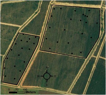
This research was carried out at a farm called El Carrascal (38°49'27.15''N, 6°46'18.39''O, 232 m. a.s.l, Datum WGS84), located near Badajoz (southwestern Spain). The area of study is 16 ha approximately and the field is divided into two separate hedgerow olive orchards (Figure 1). The climate of this area is characterised by a variation in both temperature and precipitation, typical of a Mediterranean climate. Precipitation averages less than 500 mm annually and temperature ranges between 0°C, minimum in winter, and more than 40°C, maximum in summer.
Experimental olive orchards. Soil sampling points (bigger dots) are shown.

The soil is classified as Rhodoxeralf (USDA-NRCS, 1998) and in the substrate, limestones predominate over intrusive acidic rocks. The topography is dominated by gentle hills.
Forty soil samples were collected in November 2015. Samples (Figure 1) were taken from the top layer (0–30 cm), following a stratified random sampling scheme, and their coordinates were determined with a submeter precision using a Mesa-Geode positioning system (Juniper systems, Utah, USA). Using standard procedures (Moral et al., Reference Moral, Terrón and Marques da Silva2010) the following were measured: soil apparent electrical conductivity (EC), clay, sand, and silt content, organic matter (OM), total nitrogen (TN), available phosphorous (AP) and potassium (AK), and cation exchange capacity (CEC).
The Rasch model
The probabilistic and objective Rasch model has the capacity to consolidate data, sometimes in several scale metrics, into a uniform analytical framework. In this case study, the purpose of this approach is to transcend several heterogeneous measures of nine soil properties and consolidate them into an overall variable that simplifies interpretation of soil production potential.
A key characteristic of the Rasch model is the transformation of raw data (continuous variables) to linear units (categorical variables) that operationally define a latent variable or theoretical construct. By describing soil properties in terms of uniform rating categories, unrelated properties and dimensions acquire common ordinality. Through this numerical manipulation, independent scale quantities can be expressed as common ratings ranging from low to high. The reason for changing several continuous measures to ordered rating categories is the conviction that these measures are related to an overall construct, making easier to understand their interrelations on this construct.
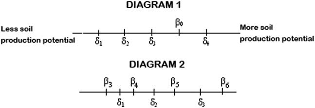
The latent variable is defined as Xni, soil production potential; βn (n=1, 2, …, 40) referring to the 40 sampling locations and δi (i=0, 1, 2, 3, 4, 5, 6, 7, 8 or 9) referring to the 9 soil properties. Xni can be regarded as a straight line along which soil properties, δi, and sample locations, βn, are located. The line ranges from less to more production potential for any sample location and is operationally defined by the 9 soil properties. The further to the right a sample point is located, the greater its production potential. The numerical gradient for this scale is called a logit (log odds) and established by estimating ordered category threshold parameters for ratings of soil properties measures that are collected at sampled locations. To estimate soil property and sample location positions, this approach was formally implemented in a Rasch model for rating scales (Andrich, Reference Andrich1988). Figure 2 shows the influence of the soil properties on soil fertility at any sampling location.
Representation of the latent variable, soil production potential, as a straight line. Diagram 1 illustrates the case of a location β0 which is influenced by the soil properties δ1, δ2, δ3, but not by δ4. Diagram 2 shows a generalization for some locations and soil properties; β3 is not influenced by any soil property; β4 is influenced by the soil property δ1; β5 is influenced by the soil properties δ1 and δ2; β6 is influenced by all soil properties, δ1, δ2 and δ3.

With the aim of analysing the raw data, different software packages were utilised. Winsteps 3.69 computer program was employed to conduct the formulation of the Rasch model. Later, the geostatistical analysis were carried out with the extension Geostatistical Analyst of the GIS software ArcGIS (version 10.3, ESRI Inc, Redlands, California, USA).
Results and discussion
Determination of soil production potential at sample points. Analysis of the Rasch measure
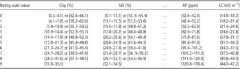
Figure 3 shows the stages to formulate the Rasch model with the aim of obtaining a measure of soil production potential at each sampling location, taking into account the different contribution of the 9 soil properties considered. Firstly, raw data were transformed to a common scale. Thus, each location was rated on a scale (0–9) for each soil property. It was assumed that the ideal percentage of each texture class was about a third of the total; consequently, the maximum categorical value (9) was assigned for an interval around 33% of clay, sand or silt content. Other rating scale values were assigned to classes with similar amplitude for each soil texture property, and the categorical values were established to correspond the highest ones with those classes that also contained the highest measures of the considered property. Table 1 presents the assignment of categorical values across properties measures (only some of them are shown). Their sum, raw score, is used to calculate the Rasch measure value (with the Winsteps program) using an unconditional maximum likelihood procedure (Linacre, Reference Linacre2000).
Stages involved in the formulation of the Rasch model.

Assignment of categorical values to some soil properties

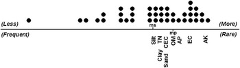
One of the main output of the Rasch model is the overall observation for all samples and soil properties displayed in tandem, in the same scale (Figure 4). In this case study, silt, clay, and TN are the most influential properties on soil production potential since they got the highest raw score and, consequently, the lowest measure. Unlike these soil properties, AK is the property with a lowest raw score and the highest measure; its influence on soil production potential is very low. Figure 4 also shows the distribution of soil samples. Although many soil samples, located to the right, have adequate propensity for production potential, others are on the left in the continuum, indicating a very low production potential (very low score). Consequently, a ranking of all soil samples according to their production potential (Rasch measure) was obtained. In this case study, no sample reached the maximum score of 90. One sample obtained 59 and ten samples reached more than 45, denoting good conditions to be potentially very fertile productive (high Rasch measure); the minimum score was only 3 points, indicating an area in which productivity shoud be very low. The establishment of a ranking according to properties of the soil samples is fundamental to find the zones in a field where the most suitable conditions of soil productivity can be expected. The fact that the mean Rasch measure for soil properties is more to the right than the mean Rasch measure for the samples indicates the existence of many locations where soil productivity potential is not optimum (Figure 4).
Soil samples and properties in the same scale. The straight line represents the latent variable: soil production potential. Distribution of soil samples (points) is above the line: to the right those more potentially productive; to the left less those less potentially productive. Soil properties are below the line: to the right less common (rare) properties, with lower influence on soil production; to the left more common (frequent) properties, with higher influence on soil production; ms and mp are the mean values of the Rasch measure for soil samples and properties respectively.

The Rasch model can provide more information through a misfiting analysis, detecting the samples which do not follow the general pattern or do not reach the expected values, known as misfits. When soil properties were considered, some misfits were found in AP. Four of these misfits are positive, denoting higher level of that soil nutrient than expected , and other three are negative, indicating lower level than expected according to the position of the sample in the ranking. Three positive misfits were also found in AK and one in EC. It is important to denote that these misfits are very scarce, due to the fact that the data fit the model reasonably, as the reliability statistics is close to 1 (0.88 and 0.84 for soil samples and properties, respectively) and the Infit and Outfit statistics are near 1 (Sekaran, Reference Sekaran2000) for both, soil samples and properties.
When the soil samples were taking into account, 14 samples displayed misfit but most of them only in one soil property. The worst case was a location with two misfits, for clay content, with a negative residual, and EC, with a positive residual. It is a location in which the expected pattern (lower clay content corresponds with lower EC) is not followed. Most of the sample misfits are related to macronutrients, mainly positive residuals, denoting higher contents than expected according to the model. The misfit analysis is a useful tool to find zones in the field where an anomaly exists, as the main deficiencies of any soil property which could affect soil production potential. Moreover, comparisons between soil samples, and so between different locations, and also site-specific amendments of any soil property can be carried out.
Spatial distribution maps of soil production potential and delineation of management zones
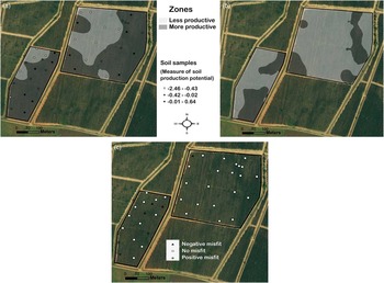
Soil production potential, characterised as the Rasch measure, at any unsampled location can be estimated with a geostatistical approach. After verifying the normality of data, a structural analysis was conducted assuming isotropy conditions as the anisotropy ratio was very low, around 1.22. A spherical theoretical variogram (range = 90.2 m; sill = 0.51; nugget effect = 0.04) was fitted to the experimental variogram. The ratio of nugget to sill (7.84%) denoted that the spatial dependence of the variable was strong (Cambardella et al., Reference Cambardella, Moorman, Novak, Parkin, Karlen, Turco and Konopka1994), which is an additional reason to apply kriging as the optimum interpolation technique. The spatial correlation described with the variograms was included in the ordinary kriging algorithm. Consequently, the kriged map from the estimated values shows the spatial distribution of the soil productivity potential in the field. If, for instance, two different MZ should be delineated, the equal-size classification technique can be utilised, resulting in the spatial distribution of the soil production potential shown in Figure 5 (more productive zones have a measure of soil production potential higher than −0.47).
a) Management zones map based on the kriged map of soil production potential. Values of the measure at the sampling locations are also indicated. b) Management zones map based on the probability map of soil production potential, considering 0.75 as the probability to exceed the measure of −0.34. c) Misfits for available phosphorous.

Probability maps can also be generated with the application of the geostatistical techniques. These maps could be used to produce MZ. For instance, a probability map of soil production potential above −0.34 (the mean value of the Rasch measure for all samples) was generated and zones with probability above 0.75 can be regarded as very productive (Figure 5). A measurement of confidence for hazard assessment of soil production potential is provided by the probabilities in this map.
The locations where misfits exist can also be visualised in a GIS. In consequence, their spatial distribution could be analysed and, additionally, site-specific amendments of any soil property can be conducted, leading to higher soil production potential. For instance, Figure 5 shows the locations where AP misfits are apparent. The positive and negative misfits denote where there is an excess or a shortage of this nutrient with respect to the optimum level to reach a higher soil production potential.
Conclusions
The application of the Rasch model with the aim of defining a measure of soil production potential, integrating different measurements of soil properties, with different units, constitutes a rational way to obtain a necessary information to delineate homogeneous zones in hedgerow olive orchards. In addition, this method can detect the influence of each soil property on the production potential for each sampling location. A classification of all soil samples according to their soil production potential was also obtained, which can provide an initial visualisation of the locations where higher or lower production potential is expected. Other useful results are the misfits, which can be utilised to detect anomalies, such as deficiencies of any soil property which could affect soil production potential.
A kriged map, showing the spatial distribution of soil production potential throughout the field, was the basis for delineating management zones. Moreover, a probability map was produced, providing information for hazard assessment of soil production potential or also for determining management zones. The combination of the Rasch model and geostatistical techniques is a powerful tool to developing an objective strategy to define site-specific management zones, the first necessary stage to implement precision farming.
Acknowledgements
This research was co-financed by the Junta de Extremadura and the European Regional Development Fund (ERDF) through the projects GR15050 (Research Group TIC008) and GR15112 (Research Group AGA001), and the projects RTA2012-00018-C02 and RTA2013-00045-C04 financed by INIA.