1 Introduction
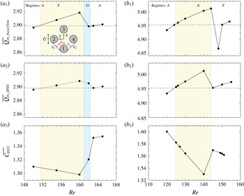
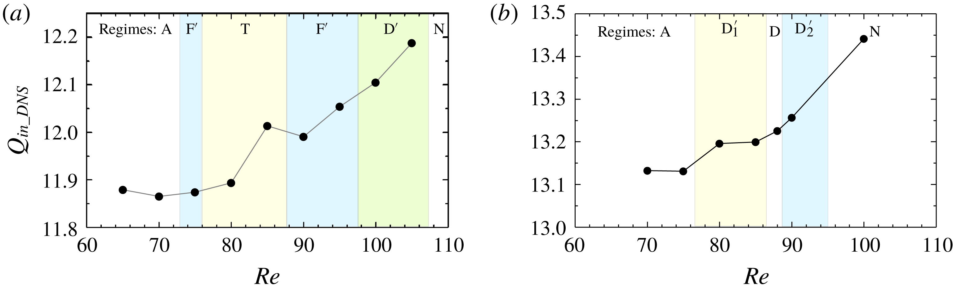
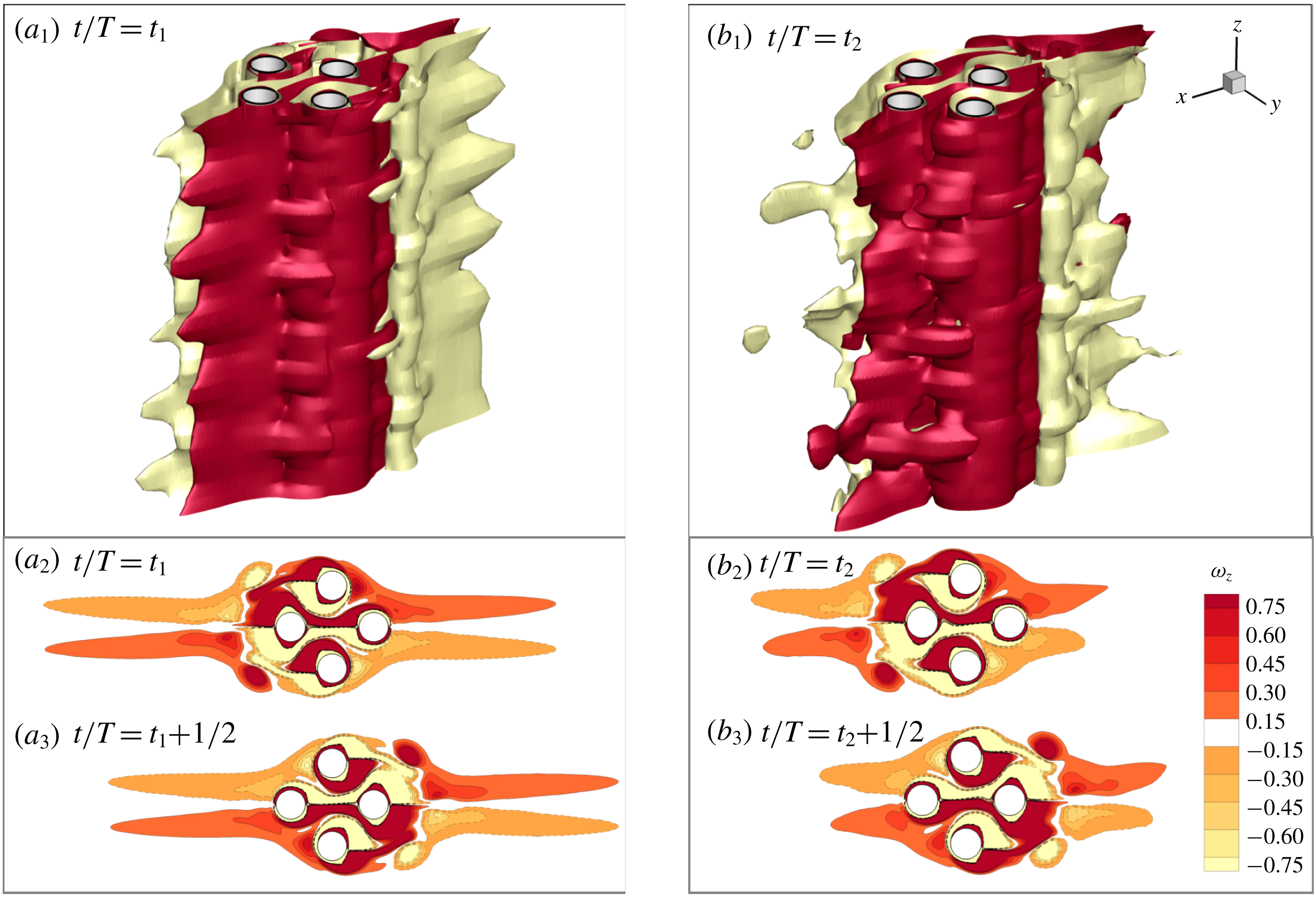
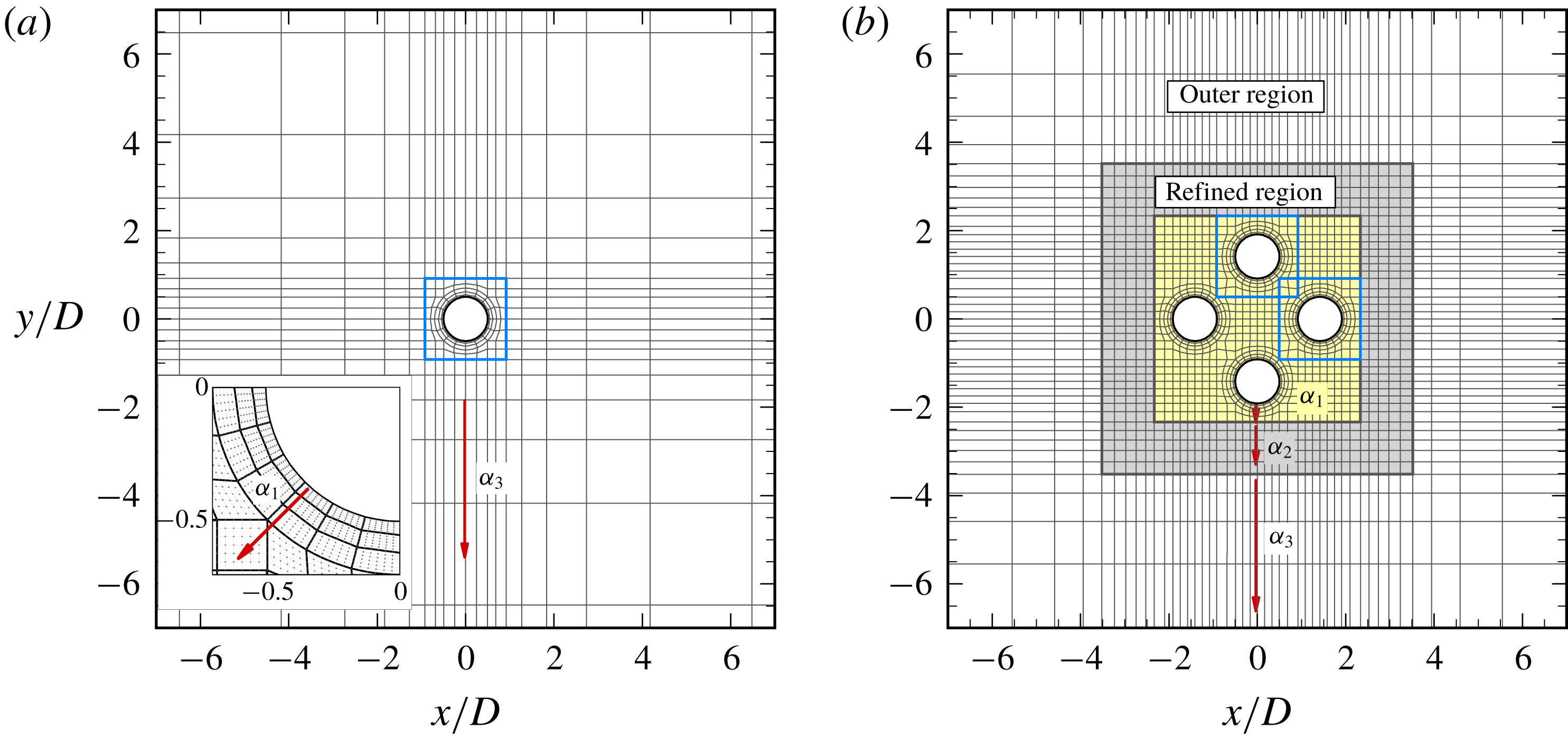
Oscillatory flow past a cluster of four cylinders has been the topic of some recent studies due to its relevance in practical engineering applications. For instance, in offshore engineering, the semi-submersible columns of floating platforms and piles of fixed platforms are normally arranged to be close to each other. Semi-submersible platforms and tension leg platforms (TLP) often have four columns that are spaced at approximately three or four diameters apart. The platforms are constantly subjected to oscillatory flow induced by surface waves (e.g. Liu et al. Reference Liu, Li, Yi and Chen2016) and prone to fatigue damages induced by cyclic wave forces. Another example is that tube heat exchangers in thermoacoustic engineering are often placed in close proximity with different arrangements, according to the availability of space (Berbish Reference Berbish2011). The flow and temperature fields around heat exchangers may be more complex under oscillatory flow conditions than that in steady flows, which are crucial in the design of the heat exchangers in marine environments (Kamsanam Reference Kamsanam2014). The flow characteristics of the present problem are not only dependent on the Keulegan–Carpenter number (KC) and the Reynolds number (Re), but also on the gap ratio (G) between the cylinders, which are defined as
 $$\begin{eqnarray}KC=\frac{U_{m}T}{D},\quad Re=\frac{U_{m}D}{\unicode[STIX]{x1D708}},\quad G=\frac{L}{D},\end{eqnarray}$$
where
 $U_{m}$
and T are the amplitude and period of the oscillatory velocity, respectively; D is the diameter of the cylinder;
 $\unicode[STIX]{x1D708}$
is the kinematic viscosity of the fluid; and L is gap distance (see figure 1). The ratio of Re and KC, known as the Stokes number, is written as
 $\unicode[STIX]{x1D6FD}=Re/\mathit{KC}=D^{2}/T\unicode[STIX]{x1D708}$
. The flow incident direction (
 $\unicode[STIX]{x1D6FC}$
) to the cylinder cluster is also significant to the flow formation. A cluster of four cylinders of equal distance in a square arrangement is one of the simplest structural arrangements, considering wake and proximity interferences and flow incident direction (Zdravkovich Reference Zdravkovich2003, pp. 995 & 1078).
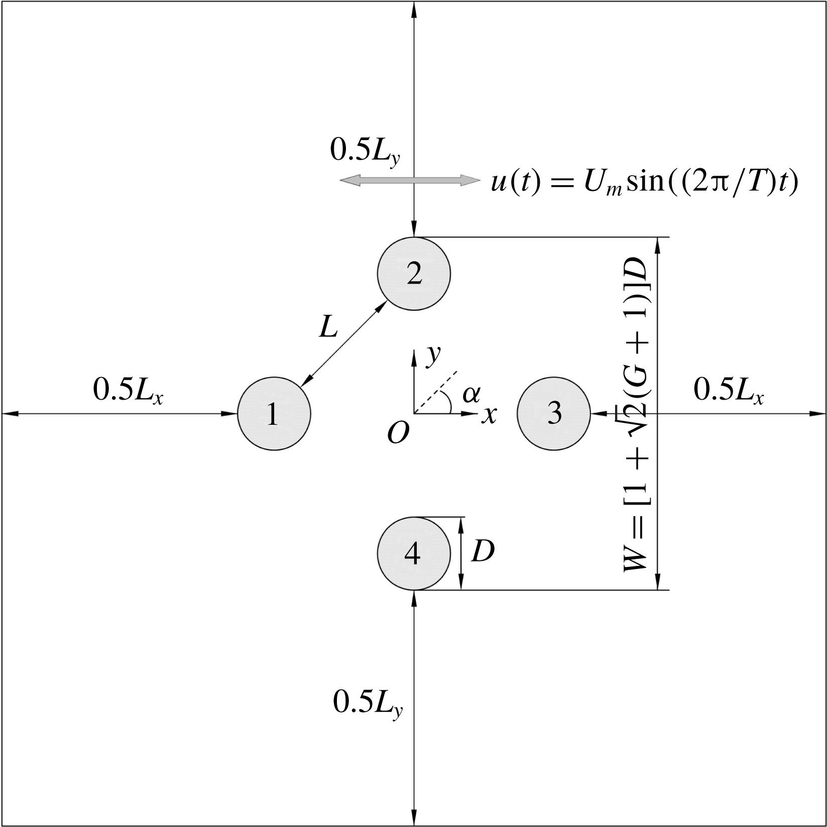
Sketch of oscillatory flow around a four-cylinder cluster in the diamond arrangement at
 $G=2$
. The cylinders are represented by four circles, i.e. C1–C4 in a clockwise direction.

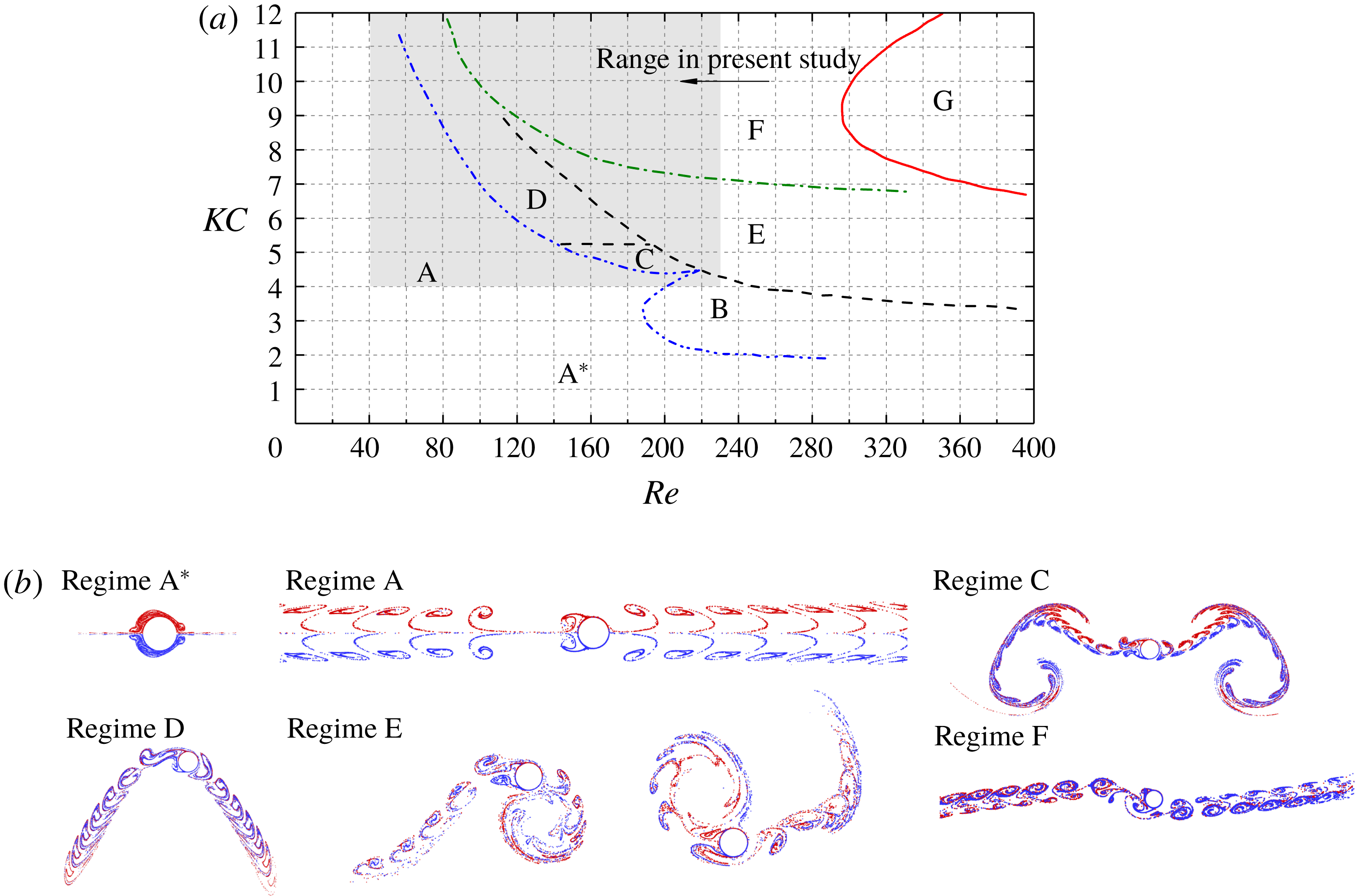
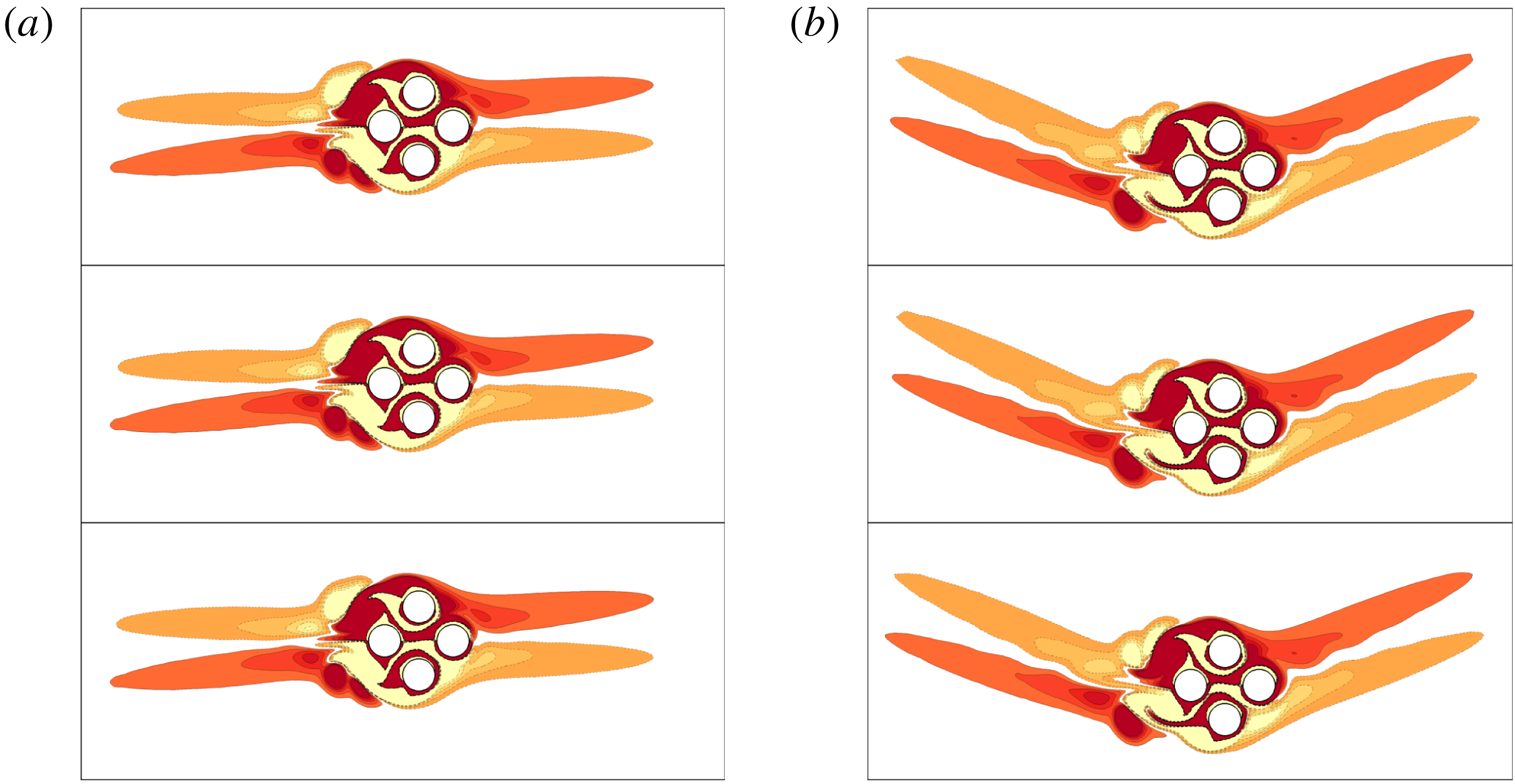
(a) Flow regime map for an isolated cylinder reproduced from Tatsuno & Bearman (Reference Tatsuno and Bearman1990) and Tong et al. (Reference Tong, Cheng, Zhao and An2015) and (b) flow features presented by streaklines by Xiong et al. (Reference Xiong, Cheng, Tong and An2018a
) for regime
 $\text{A}^{\ast }$
at
 $(KC,Re)=(3.14,165.8)$
; regime A at (11, 81.4); regime C at (5, 180); regime D at (6.28, 138.8); regime E at (6.28, 160.8); and regime F at (8.16, 220.3). The particles released from the upper and lower surfaces of the cylinder are dyed red and blue, respectively. The oscillatory flow is in the horizontal direction.

A brief review about oscillatory flow around a single cylinder is offered to facilitate further discussions on flow interactions with multiple cylinders, although more detailed reviews can be found in a number of recent studies (e.g. Elston, Blackburn & Sheridan Reference Elston, Blackburn and Sheridan2006; Deng & Caulfield Reference Deng and Caulfield2015; Tong et al.
Reference Tong, Cheng, Xiong, Draper, An and Lou2017; Xiong et al.
Reference Xiong, Cheng, Tong and An2018a
). At relatively low Re (
 ${\leqslant}$
1200) and KC (
 ${\leqslant}$
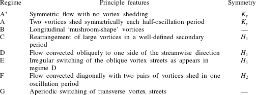
15), the flow exhibits a number of distinct features. Tatsuno & Bearman (Reference Tatsuno and Bearman1990) classified these flow features into eight regimes (regimes
 $\text{A}^{\ast }$
and A to G) in a parameter space of
 $KC=1.6$
–15 and
 $\unicode[STIX]{x1D6FD}=5$
–160 (
 $Re\leqslant 1200$
), which are briefly listed in table 1. The flow regime map in the range of
 $KC\leqslant 12$
and
 $Re\leqslant 400$
and the flow visualization through streaklines are reproduced in figure 2 based on Tong et al. (Reference Tong, Cheng, Zhao and An2015) and Xiong et al. (Reference Xiong, Cheng, Tong and An2018a
), respectively. The two-dimensional (2-D) states of symmetry of the cross-sectional flows, as summarized by Elston, Sheridan & Blackburn (Reference Elston, Sheridan and Blackburn2004), are listed below.
 $$\begin{eqnarray}\displaystyle \mathit{Reflection}~\mathit{symmetry}~K_{y}:\quad & & \displaystyle \unicode[STIX]{x1D714}_{z}(x,y,t)=-\unicode[STIX]{x1D714}_{z}(x,-y,t),\end{eqnarray}$$
 $$\begin{eqnarray}\displaystyle \mathit{Spatio}\text{-}\mathit{temporal}~\mathit{symmetry}~H_{1}:\quad & & \displaystyle \unicode[STIX]{x1D714}_{z}(x,y,t)=-\unicode[STIX]{x1D714}_{z}(-x,y,t+T/2),\end{eqnarray}$$
 $$\begin{eqnarray}\displaystyle \mathit{Spatio}\text{-}\mathit{temporal}~\mathit{symmetry}~H_{2}:\quad & & \displaystyle \unicode[STIX]{x1D714}_{z}(x,y,t)=\unicode[STIX]{x1D714}_{z}(-x,-y,t+T/2),\end{eqnarray}$$
where x and y are Cartesian coordinates with x being the direction of flow oscillations, and vorticity
 $\unicode[STIX]{x1D714}_{z}$
is the curl of the 2-D velocity components
 $U=(u,v)$
,
 $$\begin{eqnarray}\displaystyle \unicode[STIX]{x1D714}_{z}=\frac{\unicode[STIX]{x2202}v}{\unicode[STIX]{x2202}x}-\frac{\unicode[STIX]{x2202}u}{\unicode[STIX]{x2202}y}. & & \displaystyle\end{eqnarray}$$
Rich flow features are also discovered in oscillatory flow around a cluster of multiple cylinders, although the relevant studies are less extensive. Williamson (Reference Williamson1985) carried out an experimental study of flow around two sinusoidally oscillating cylinders in still water and found that the flow regimes as identified in table 1 may change due to the interaction between cylinders. Flow regimes around two cylinders of side-by-side, tandem and staggered arrangements relative to the direction of flow oscillation have been studied numerically (Chern et al.
Reference Chern, Kanna, Lu, Cheng and Chang2010; Yang et al.
Reference Yang, Cheng, An, Bassom and Zhao2013; Zhao & Cheng Reference Zhao and Cheng2014). Zhao & Cheng (Reference Zhao and Cheng2014) employed 2-D direct numerical simulation (DNS) to investigate oscillatory flow past a two-cylinder system with both tandem and side-by-side arrangements at
 $Re=100$
and 150 with
 $G=0.5$
–5 and
 $KC=1$
–12. A number of flow regimes, including those named using combinations of the existing flow regimes for a single cylinder and newly found regimes such as the gap vortex shedding (GVS) regime, are mapped out in the KC–
 $\unicode[STIX]{x1D6FD}$
plane. The occurrence of the new flow regimes is dependent on G.
Flow features of eight flow regimes for a single circular cylinder (Tatsuno & Bearman Reference Tatsuno and Bearman1990; Honji Reference Honji2006).

Oscillatory flow around a cluster of four cylinders has not been extensively studied. Anagnostopoulos & Dikarou (Reference Anagnostopoulos and Dikarou2011, Reference Anagnostopoulos and Dikarou2012) analysed the links between the appearance of periodic and aperiodic hydrodynamic forces and flow structures through simulating oscillatory flow past four circular cylinders in a square arrangement at
 $\unicode[STIX]{x1D6FD}=50$
and
 $KC=0.2$
–10 with
 $G=1.5$
and 1.75. Chern, Shiu & Horng (Reference Chern, Shiu and Horng2013) employed 2-D immersed boundary modelling method for oscillatory flow past a cluster of four cylinders with flow inclined angle (
 $\unicode[STIX]{x1D6FC}$
) at
 $0^{\circ }$
and
 $45^{\circ }$
(square and diamond arrangements, respectively) and
 $G=1$
–4. The results showed that the in-line force coefficient is less sensitive than the lift coefficient to
 $\unicode[STIX]{x1D6FC}$
and G. Tong et al. (Reference Tong, Cheng, Zhao and An2015) classified flow regimes of oscillatory flow around four cylinders in a square arrangement over the parameter ranges
 $KC=1$
–12 and
 $Re=20$
–200. Six types of flow regimes with symmetries (specified by (1.2) to (1.4)) and a series of symmetry-breaking regimes are mapped out in the KC–Re plane. Tong et al. (Reference Tong, Cheng, Zhao and An2015) found that the reflection symmetry flow dominates the regime maps, especially at small gap ratios (
 $G=0.5$
and 1) owing to the stabilization effect induced by the jet-like flow passing through the gap between two pairs of tandem cylinders. It was found that the cylinder cluster behaves in a similar manner to a single porous body at small gap ratios, and therefore the flow fields resemble those around a single cylinder. Interactions of local vortices around each cylinder have strong influence on the global flow structures at
 $G=2$
and become weak at
 $G=4$
.
Oscillatory flow around a cluster of cylinders is also dependent on the flow incident direction relative to the cylinder cluster. Tong, Cheng & Zhou (Reference Tong, Cheng and Zhou2014b
) investigated flow features and the variation of forces for oscillatory flow around four cylinders in a diamond arrangement (
 $\unicode[STIX]{x1D6FC}=45^{\circ }$
) at
 $Re=150$
over the parameter ranges of
 $KC=4$
–9 and
 $G=1$
–3. A few flow features were demonstrated through streaklines and interpreted through temporal variations of lift coefficient on one of the side cylinders. In general, they found, through the temporal variations of the lift coefficient, that oscillatory flow around four cylinders in a diamond arrangement is more chaotic than the corresponding flow around a square arrangement due to the influences of asymmetric vortex shedding from individual cylinders and the interactions of the shed vortices. Since only a single
 $Re=150$
was investigated in Tong et al. (Reference Tong, Cheng and Zhou2014b
), no flow regime maps were provided. In addition, no attempts were made to investigate the physical mechanisms of a number of interesting (quasi-periodic and chaotic) features displayed by the temporal variations of lift and their intrinsic links with detailed flow features, due to the limit on the length of the paper.
The present paper can be considered as an extension to the study reported by Tong et al. (Reference Tong, Cheng and Zhou2014b ). We are particularly interested in exploring (i) the flow features and physical mechanisms that are responsible for the quasi-periodic and chaotic features of the temporal variations of lift reported in Tong et al. (Reference Tong, Cheng and Zhou2014b ), (ii) the similarity and difference (influence of flow incident angle) between oscillatory flows around four cylinders in square and diamond arrangements and (iii) the influence of Re and KC on the flow in a parameter space comparable to that reported by Tong et al. (Reference Tong, Cheng, Zhao and An2015) for a square arrangement.
The remainder of the paper is organized in the following manner. In § 2, the governing equations, numerical model, linear Floquet stability analysis and concepts of phase dynamics are introduced. In § 3, the regime maps are presented, together with detailed flow and force features in the respective regimes. A brief discussion on the so called ‘holes’ in the regime maps and major differences between a square arrangement and a diamond arrangement is offered in § 4, along with a brief discussion on three-dimensionality effect. Finally, major conclusions are drawn in § 5.
2 Numerical approach
2.1 Numerical method
Figure 1 shows a sketch of the cylinder cluster investigated in the present study. A reference Cartesian coordinate system
 $(x,y)$
is defined with its origin being placed at the centre of the cylinder cluster. The governing equations for the flow are the non-dimensional continuity and incompressible Navier–Stokes (N–S) equations,
 $$\begin{eqnarray}\displaystyle & \displaystyle \frac{\unicode[STIX]{x2202}u_{i}}{\unicode[STIX]{x2202}x_{i}}=0, & \displaystyle\end{eqnarray}$$
 $$\begin{eqnarray}\displaystyle & \displaystyle \frac{\unicode[STIX]{x2202}u_{i}}{\unicode[STIX]{x2202}t}+u_{j}\frac{\unicode[STIX]{x2202}u_{i}}{\unicode[STIX]{x2202}x_{j}}=-\frac{1}{\unicode[STIX]{x1D70C}}\frac{\unicode[STIX]{x2202}p}{\unicode[STIX]{x2202}x_{i}}+\frac{1}{Re}\frac{\unicode[STIX]{x2202}^{2}u_{i}}{\unicode[STIX]{x2202}{x_{j}}^{2}},\quad (i,j=1,2), & \displaystyle\end{eqnarray}$$
 $(x_{1},x_{2})=(x,y)$
,
 $u_{i}$
is the velocity component corresponding to
 $x_{i}$
,
 $t$
is time,
 $p$
is pressure and
 $\unicode[STIX]{x1D70C}$
is fluid density. The diameter of cylinder
 $D$
and the amplitude of oscillatory velocity
 $U_{m}$
are used to normalize the above equations.
The governing equations are solved by using a spectral/hp element method that is embedded in an open-source software package Nektar++ (Cantwell et al.
Reference Cantwell, Moxey, Comerford, Bolis, Rocco, Mengaldo, De Grazia, Yakovlev, Lombard and Ekelschot2015). The total mesh resolution in Nektar++ is determined by the distribution of h-type elements and the interpolation order
 $N_{p}$
for the p-type refinement. In the present study, sixth-order Lagrange polynomials are used on Gauss–Lobatto–Legendre quadrature points. A second-order time integration method, a velocity correction scheme and a Galerkin formulation are employed for all the present simulations. Further details can be found in Karniadakis, Israeli & Orszag (Reference Karniadakis, Israeli and Orszag1991), Guermond & Shen (Reference Guermond and Shen2003), Blackburn & Sherwin (Reference Blackburn and Sherwin2004) and Vos et al. (Reference Vos, Eskilsson, Bolis, Chun, Kirby and Sherwin2011).
2.2 Computational domain and boundary conditions
As shown in figure 1, a square computational domain of size
 $(L_{x}+W)\times (L_{y}+W)$
is adopted for the simulations, where
 $L_{x}=L_{y}=100D$
are the lengths of the outer domain in the x- and y-directions, respectively, and
 $W=[1+\sqrt{2}(G+1)]D$
is the projected width of the cylinder cluster perpendicular to the flow direction. The size of a square computational domain changes from 103.12D to 108.07D for the G values investigated in the present study. This setting leads to a blockage ratio ranging from 2.78 to 2.91 % for different gap ratios, which is similar to those reported in previous studies for oscillatory flows, e.g. 1.67 % and 3.33 % for two circular cylinders (Zhao & Cheng Reference Zhao and Cheng2014) and 2 % for a cluster of four cylinders (Tong et al.
Reference Tong, Cheng, Zhao and An2015).
The boundary conditions of the outer boundaries of the domain are specified as
 $u_{\infty }(t)=U_{m}\sin (\unicode[STIX]{x1D714}t)$
and
 $v_{\infty }=0$
, where
 $\unicode[STIX]{x1D714}=2\unicode[STIX]{x03C0}f_{u}$
with
 $f_{u}$
being the frequency of flow oscillation (
 $=1/T$
). The no-slip boundary condition is defined on the surface of the cylinders. A high-order Neumann boundary condition for pressure field, as suggested by Karniadakis et al. (Reference Karniadakis, Israeli and Orszag1991) and Blackburn & Sherwin (Reference Blackburn and Sherwin2004), is specified on all the boundaries involved in this simulation. It should be noted that in Nektar++ one degree of freedom is pinned to zero to avoid singular pressure-Poison problem (Bolis Reference Bolis2013). Zero initial conditions for velocities and pressure are specified.
The time-step size
 $\unicode[STIX]{x0394}t$
for each case is chosen to be
 $\unicode[STIX]{x0394}t=0.001$
, based on the Courant–Friedrichs–Lewy (CFL) stability criterion, which is defined as
 $$\begin{eqnarray}\text{CFL}=\frac{|U|\unicode[STIX]{x0394}t}{\unicode[STIX]{x0394}l},\end{eqnarray}$$
where
 $|U|$
is the magnitude of the velocity in a cell and
 $\unicode[STIX]{x0394}l$
is the cell size in the direction of the velocity. The maximum value of CFL is kept below 0.5 for all the simulations conducted in the present study.
The details of a mesh dependence check are presented in appendix A.
2.3 Linear (Floquet) stability analysis
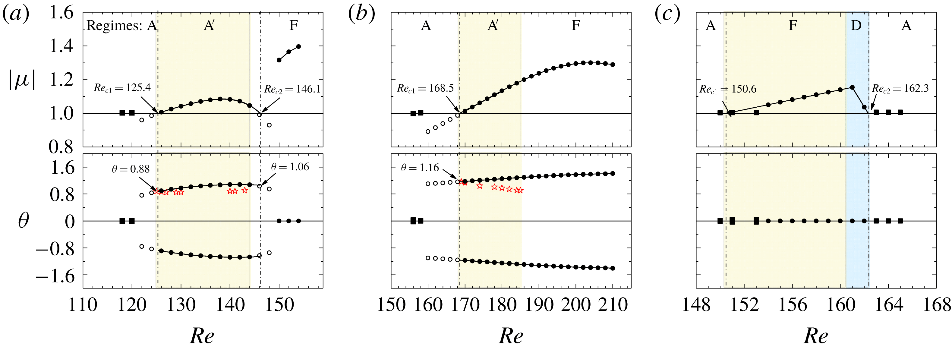
Linear (Floquet) stability analysis is conducted to ascertain an observation that certain synchronous or quasi-periodic flows occur at unexpected locations in the KC–Re space.
Floquet stability analysis examines the evolution of velocity and pressure perturbations
 $u_{i}^{\prime }(x,y,t)$
and
 $p_{i}^{\prime }(x,y,t)$
to a T-periodic base flow
 $u_{i}(x,y,t)$
by solving the linearized continuity and N–S equations for velocity and pressure perturbations
 $$\begin{eqnarray}\displaystyle & \displaystyle \frac{\unicode[STIX]{x2202}u_{i}^{\prime }}{\unicode[STIX]{x2202}x_{i}}=0, & \displaystyle\end{eqnarray}$$
 $$\begin{eqnarray}\displaystyle & \displaystyle \frac{\unicode[STIX]{x2202}u_{i}^{\prime }}{\unicode[STIX]{x2202}t}=-u_{j}\frac{\unicode[STIX]{x2202}u_{i}^{\prime }}{\unicode[STIX]{x2202}x_{j}}-u_{j}^{\prime }\frac{\unicode[STIX]{x2202}u_{i}}{\unicode[STIX]{x2202}x_{j}}-\frac{1}{\unicode[STIX]{x1D70C}}\frac{\unicode[STIX]{x2202}p^{\prime }}{\unicode[STIX]{x2202}x_{i}}+\frac{1}{Re}\frac{\unicode[STIX]{x2202}^{2}u_{i}^{\prime }}{\unicode[STIX]{x2202}{x_{j}}^{2}},\quad (i,j=1,2). & \displaystyle\end{eqnarray}$$
The right-hand side of (2.3b
) is T-periodic with respect to the base flow because of the linearized advection term, and therefore can be solved numerically by iterating on the T-periodic base flow (Barkley & Henderson Reference Barkley and Henderson1996; Elston et al.
Reference Elston, Sheridan and Blackburn2004, Reference Elston, Blackburn and Sheridan2006). The solutions of
 $u_{i}^{\prime }(x,y,t)$
can be written as a sum of components
 $u_{i}^{\prime }(x,y,t)=\tilde{u} _{i}(x,y,t)\exp (\unicode[STIX]{x1D70E}t)$
, where
 $\tilde{u} _{i}(x,y,t)$
is also a T-periodic Floquet eigenfunction and the complex number
 $\unicode[STIX]{x1D70E}$
is the Floquet exponent (Barkley & Henderson Reference Barkley and Henderson1996). The flow becomes unstable if the Floquet multiplier,
 $\unicode[STIX]{x1D707}\equiv \exp (\unicode[STIX]{x1D70E}T)$
, crosses the unit circle (i.e.
 $|\unicode[STIX]{x1D707}|>1$
). As discussed by Elston et al. (Reference Elston, Sheridan and Blackburn2004), the flow becomes quasi-periodic if
 $\unicode[STIX]{x1D707}=\exp (\pm \text{i}\unicode[STIX]{x1D703})$
is a complex-conjugate pair. The relationship between the phase angle
 $\unicode[STIX]{x1D703}$
and the secondary period
 $T_{s}$
is given as
 $T_{s}\approx 2\unicode[STIX]{x03C0}/\unicode[STIX]{x1D703}$
. To examine the breaking of
 $K_{y}$
symmetry, the periodic base flow is obtained by solving (2.1) in the upper half of the computational domain
 $(y\geqslant 0)$
with symmetry boundary conditions on the
 $y=0$
boundary (Elston et al.
Reference Elston, Sheridan and Blackburn2004, Reference Elston, Blackburn and Sheridan2006). Other boundary conditions and the mesh resolution used in the Floquet analysis are identical to those employed in DNS. The base flow is calculated for at least 200T to obtain a fully developed periodic solution. After that, this base flow is projected onto the full computational domain according to the reflection symmetry condition in (1.2) and 64 equi-spaced time slices over a flow oscillation period are used for the Floquet analysis. This analysis method is identical to the method employed by Elston et al. (Reference Elston, Sheridan and Blackburn2004, Reference Elston, Blackburn and Sheridan2006).
2.4 Quantitative identification of the flow regimes
For each G, flow regimes are mapped out based on the temporal and spatial features of the flow field (including vorticity contours and streaklines), temporal variations of the total lift coefficient, the Lissajous phase diagram of the total in-line and lift coefficients, spectra of total lift coefficient and the phase dynamics between the total lift coefficient and the far-field flow velocity.
The total in-line and lift coefficients,
 $C_{x}$
and
 $C_{y}$
respectively, are defined as
 $$\begin{eqnarray}\displaystyle C_{x}=\frac{F_{x}}{\frac{1}{2}\unicode[STIX]{x1D70C}{U_{m}}^{2}D},\quad C_{y}=\frac{F_{y}}{\frac{1}{2}\unicode[STIX]{x1D70C}{U_{m}}^{2}D}, & & \displaystyle\end{eqnarray}$$
 $$\begin{eqnarray}\displaystyle F_{x}=\frac{1}{4}\mathop{\sum }_{i=1}^{4}F_{xi},\quad F_{y}=\frac{1}{4}\mathop{\sum }_{i=1}^{4}F_{yi}, & & \displaystyle\end{eqnarray}$$
where
 $F_{xi}$
and
 $F_{yi}$
are the in-line and transverse forces on a single cylinder (i denotes the cylinder number), which are obtained by integrating the pressure and shear stress along the cylinder surface.
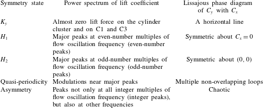
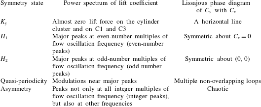
Classification of symmetric states through power spectrum and phase diagram.
The root-mean-square (r.m.s.) in-line coefficient
 $C_{xi}^{\prime }$
and lift coefficient
 $C_{yi}^{\prime }$
for a single cylinder are defined as
 $$\begin{eqnarray}C_{xi}^{\prime }=\sqrt{\frac{1}{M}\mathop{\sum }_{m=1}^{M}{C_{xi}}^{2}},\quad C_{yi}^{\prime }=\sqrt{\frac{1}{M}\mathop{\sum }_{m=1}^{M}{C_{yi}}^{2}},\end{eqnarray}$$
where
 $M$
is the sampling size of the statistics,
 $C_{xi}$
and
 $C_{yi}$
are the individual in-line and lift coefficients on each cylinder in the same manner as defined in (2.4). The r.m.s. lift and in-line coefficients on C1 and C3 (in-line) and C2 and C4 (side) cylinder pairs, denoted as
 $\overline{C_{y13}^{\prime }}$
and
 $\overline{C_{y24}^{\prime }}$
, and
 $\overline{C_{x13}^{\prime }}$
and
 $\overline{C_{x24}^{\prime }}$
correspondingly, are determined by averaging the r.m.s. force coefficients on individual cylinders in the pairs to obtain representative r.m.s. lift and in-line coefficients on the pairs. The
 $C_{x}^{\prime }$
and
 $C_{y}^{\prime }$
are the r.m.s. values of
 $C_{x}$
and
 $C_{y}$
through the same manner as that defined in (2.6). Flow symmetry states are identified through both Lissajous phase diagram of
 $C_{y}$
with
 $C_{x}$
and the occurrence of dominant peaks in the
 $C_{y}$
spectrum. The characteristics of the symmetry states and the power spectra of
 $C_{y}$
are listed in table 2 for reference (Tong et al.
Reference Tong, Cheng, Xiong, Draper, An and Lou2017; Xiong et al.
Reference Xiong, Cheng, Tong and An2018a
). Detailed features will be interpreted in § 3.
The streaklines are generated by releasing massless particles at 80 equi-spaced points around the circle perimeter at a distance of 0.01D from the cylinder surface and a time interval of
 $1/8$
times of the flow oscillation period (where the integration time step is
 $KC/8$
) lasting for at least 10T. The massless particles released from different cylinders are set to different colours (orange, red, green and blue for C1–C4, respectively) to visualize the mixing of particles as a consequence of flow interactions. It has been checked (results not shown here) that further reduction of the releasing time interval from
 $KC/8$
to
 $KC/32$
has little influence on the streakline patterns.
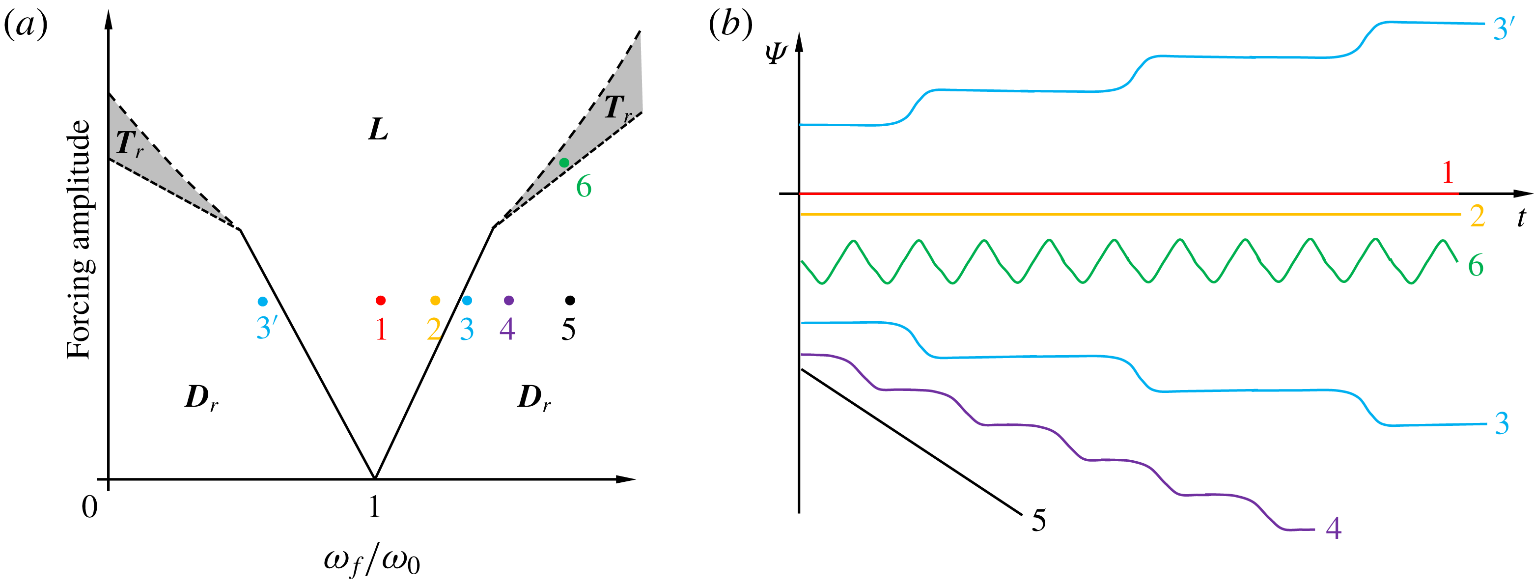
(a) Phase dynamics for a forced van der Pol oscillator, on the plane of forcing amplitude against the normalized forcing frequency (
 $\unicode[STIX]{x1D714}_{f}/\unicode[STIX]{x1D714}_{0}$
). The phase differences between the response of the oscillator and the external forcing are shown in (b); these values are indicated in (a) by points 1–6 in the three regions, namely
 $\boldsymbol{L}$
,
 $\boldsymbol{T}_{\boldsymbol{r}}$
and
 $\boldsymbol{D}_{\boldsymbol{r}}$
. The bifurcation map in (a) is reproduced from figure 1 in Li & Juniper (Reference Li and Juniper2013) and the time traces of phase dynamics in (b) are reproduced from figure 3.8 in Pikovsky, Rosenblum & Kurths (Reference Pikovsky, Rosenblum and Kurths2003).

2.5 Phase dynamics
Quasi-periodic flows have been widely observed in the steady/oscillatory flow around a fixed bluff body (e.g. Elston et al. Reference Elston, Blackburn and Sheridan2006; Burattini & Agrawal Reference Burattini and Agrawal2013; Deng & Caulfield Reference Deng and Caulfield2015) and in the flow around bluff bodies under forced oscillation (e.g. Leontini, Lo Jacono & Thompson Reference Leontini, Lo Jacono and Thompson2011; Tang et al. Reference Tang, Cheng, Tong, Lu and Zhao2017). However, the synchronization mechanism between the quasi-periodic behaviour and ambient flows has not been fully investigated. Previous investigations of quasi-periodic phenomena in a self-excited jet (Li & Juniper Reference Li and Juniper2013) and thermoacoustic system (Kashinath, Li & Juniper Reference Kashinath, Li and Juniper2018) are demonstrated through the use of synchronization theory. Some of the quasi-periodic flow characteristics observed in the present study are interpreted in detail through the existing synchronization theory of a forced self-sustained oscillator, which is adopted for the first time in bluff-body flows, to the best knowledge of the authors. The incoming oscillatory flow constitutes the external forcing and the flow formed around the cylinder cluster (or the resulting lift force on the cylinder cluster or individual cylinders) is considered as the response to the external forcing.
According to Pikovsky et al. (Reference Pikovsky, Rosenblum and Kurths2003), the synchronization state of a forced oscillator is dependent on the amplitude of external forcing and the difference between the natural frequency and the frequency of external forcing, which is termed frequency detuning in the literature. The three synchronization states:
 $\boldsymbol{L}$
for phase locking,
 $\boldsymbol{T}_{\boldsymbol{r}}$
for phase trapping,
 $\boldsymbol{D}_{\boldsymbol{r}}$
for phase drifting (including phase slipping), and the corresponding phase dynamics in the response of a forced van der Pol oscillator are illustrated in figure 3 (Li & Juniper Reference Li and Juniper2013), where
 $\unicode[STIX]{x1D714}_{0}$
and
 $\unicode[STIX]{x1D714}_{f}$
denote the natural angular frequency of the system and the angular frequency of external forcing, respectively, and
 $\unicode[STIX]{x1D6F9}$
is the phase difference between the response of the oscillator and the external forcing. In the perfect synchronization regions
 $\boldsymbol{L}$
(points 1 and 2),
 $\unicode[STIX]{x1D6F9}$
is locked to a constant value. This behaviour is referred to as phase locking. The phase dynamics of points 3 and 4 near boundaries of
 $\boldsymbol{L}$
and
 $\boldsymbol{D}_{\boldsymbol{r}}$
is characterized by phase drifting and slipping where
 $\unicode[STIX]{x1D6F9}$
remains nearly constant (a near synchronization state) over a long period of time, followed by a sudden change of
 $\unicode[STIX]{x1D6F9}$
. While further away from the boundaries (point 5), no phase slip is observed in the time traces of
 $\unicode[STIX]{x1D6F9}$
. In the phase trapping region
 $\boldsymbol{T}_{\boldsymbol{r}}$
(between
 $\boldsymbol{L}$
and
 $\boldsymbol{D}_{\boldsymbol{r}}$
at large forcing amplitude) (point 6),
 $\unicode[STIX]{x1D6F9}$
oscillates around a constant value with the mean time derivative of the phase difference
 $\langle \dot{\unicode[STIX]{x1D6F9}}\rangle =0$
(line 6), where
 $\langle \cdot \rangle$
denotes a time-averaged quantity and the dot accent denotes the time derivative hereafter.
2.5.1 Phase analysis
In the present study, several frequencies of flow responses are defined to interpret the phase states of different flow regimes:
(i)
 $f_{y}$
, the response frequency, is the frequency of overall flow response and is identified as the frequency corresponding to the dominant peak component in the
$C_{y}$
spectrum. The corresponding period of
$f_{y}$
is defined as
$T_{y}$
.
(ii)
$f_{l}$
, the fundamental lift frequency, is a frequency employed in the phase analysis of quasi-periodic flows and is obtained by rounding
$f_{y}$
to the nearest integer. The
$f_{l}$
of quasi-periodic flows is actually the fundamental lift frequency of corresponding synchronous flows as defined by Williamson (Reference Williamson1985). The corresponding period of
$f_{l}$
is defined as
$T_{l}$
. The flow related to
$f_{l}$
is defined as local flow in the following discussions.(iii)
$f_{s}$
, the secondary frequency, is inherent in quasi-periodic flows and represents the frequency of a slow flow process (termed secondary flow hereafter) in the overall flow response. The corresponding period and angular frequency of
$f_{s}$
are defined as
$T_{s}$
and
$\unicode[STIX]{x1D714}_{s}$
, respectively. The secondary flow is considered as a disturbance to the local flow response by default in the following analysis.


The flow mechanisms associated with the behaviours observed in quasi-periodic flows are investigated with the aid of the phase dynamics between the flow response
 $(C_{y}(t))$
and external forcing
 $(u_{\infty }(t))$
. The phase difference is defined as
 $$\begin{eqnarray}\displaystyle \unicode[STIX]{x1D6F9}(t)=\unicode[STIX]{x1D6F9}_{y}(t)-\unicode[STIX]{x1D6F9}_{u}(t), & & \displaystyle\end{eqnarray}$$
where
 $\unicode[STIX]{x1D6F9}_{y}(t)$
is the instantaneous phase of
 $C_{y}(t)$
determined from the Hilbert transform (Pikovsky et al.
Reference Pikovsky, Rosenblum and Kurths2003). Assuming periodic variations of
 $C_{y}(t)$
with a period of
 $T_{y}$
, we have
 $$\begin{eqnarray}\displaystyle \unicode[STIX]{x1D6F9}_{y}(t)=2\unicode[STIX]{x03C0}f_{y}t+\unicode[STIX]{x1D719}_{i}(t), & & \displaystyle\end{eqnarray}$$
where
 $\unicode[STIX]{x1D719}_{i}(t)$
represents all other frequency contents of
 $C_{y}(t)$
.
 $\unicode[STIX]{x1D6F9}_{u}(t)$
represents the instantaneous phase of external forcing and is given as
 $$\begin{eqnarray}\displaystyle \unicode[STIX]{x1D6F9}_{u}(t)=2\unicode[STIX]{x03C0}f_{l}t. & & \displaystyle\end{eqnarray}$$
A running time average of
 $\unicode[STIX]{x1D6F9}(t)$
over a period of time
 $T_{a}$
is defined as
 $$\begin{eqnarray}\displaystyle \overline{\unicode[STIX]{x1D6F9}_{T_{a}}}=\langle \unicode[STIX]{x1D6F9}(t^{\prime })\rangle _{T_{a}}=\frac{1}{T_{a}}\int _{t_{0}}^{t_{0}+T_{a}}\unicode[STIX]{x1D6F9}(t)\,\text{d}t, & & \displaystyle\end{eqnarray}$$
where
 $\langle \cdot \rangle _{T_{a}}$
denotes the time-averaged results over a period
 $T_{a}$
.
2.5.2 The circle maps
We are particularly interested in the interaction of the local and secondary flow responses observed in quasi-periodic flows. The secondary flow is a slow process in comparison with the local flow and
 $T_{s}$
is normally much larger than
 $T_{l}$
. The period of local flow is of the same order of magnitude as the period of incoming flow through
 $T=nT_{l}$
, where
 $n$
is an integer (Williamson Reference Williamson1985; Sumer & Fredsøe Reference Sumer and Fredsøe1997). If the quotient
 $T_{s}/T_{l}$
is rational, the slow process is periodic with period
 $T_{l}$
, which locates in the region
 $\boldsymbol{L}$
or
 $\boldsymbol{T}_{\boldsymbol{r}}$
. Otherwise it is quasi-periodic in region
 $\boldsymbol{D}_{\boldsymbol{r}}$
.
Two methods of observation are employed to investigate the interaction process in the present study. The first method observes the response of secondary flow process by undertaking a stroboscopic mapping of the slow process through time interval
 $T$
, which is equivalent to considering the local flow as the external forcing. The second method is a reversal of the first method, i.e. observing the response of local flow process by considering the secondary flow as the external forcing. The second method is implemented by taking a stroboscopic mapping of the local flow process through time interval
 $T_{s}$
. The phase equations for both methods of observation are outlined below. Following the first method, the phase equation of the secondary flow in the vicinity of the synchronization can be written as (Pikovsky et al.
Reference Pikovsky, Rosenblum and Kurths2003, pp. 201)
 $$\begin{eqnarray}\frac{\text{d}\unicode[STIX]{x1D719}_{s}}{\text{d}t}=\unicode[STIX]{x1D714}_{s}+\unicode[STIX]{x1D700}Q(\unicode[STIX]{x1D719}_{s},t),\end{eqnarray}$$
where
 $\unicode[STIX]{x1D719}_{s}$
is the phase of the secondary flow process,
 $\unicode[STIX]{x1D700}$
is a small parameter, and
 $Q(\unicode[STIX]{x1D719}_{s},t)$
represents a
 $2\unicode[STIX]{x03C0}$
-periodic forcing function of
 $\unicode[STIX]{x1D719}_{s}$
and a
 $T$
-periodic function of
 $t$
. Thus, the phase space represented by (2.11) is a two-dimensional torus
 $0\leqslant \unicode[STIX]{x1D719}_{s}\leqslant 2\unicode[STIX]{x03C0}$
,
 $0\leqslant t\leqslant T$
, which can be reduced to a one-dimensional mapping explicitly. For a fixed time
 $t=t_{0}$
, a smooth invertible circle map is defined (Pikovsky et al.
Reference Pikovsky, Rosenblum and Kurths2003, pp. 201):
 $$\begin{eqnarray}\displaystyle \unicode[STIX]{x1D719}_{s}^{N+1}=\unicode[STIX]{x1D719}_{s}^{N}+2\unicode[STIX]{x03C0}T/T_{s}+\unicode[STIX]{x1D700}F(\unicode[STIX]{x1D719}_{s}^{N}), & & \displaystyle\end{eqnarray}$$
where
 $\unicode[STIX]{x1D719}_{s}^{N}$
refers to the phase of secondary flow in
 $N$
th flow oscillation period. Following the same method of mapping, the circle map for the second method of observation can be written as
 $$\begin{eqnarray}\unicode[STIX]{x1D719}^{N+1}=\unicode[STIX]{x1D719}^{N}+2\unicode[STIX]{x03C0}T_{s}/T_{l}+\unicode[STIX]{x1D700}G(\unicode[STIX]{x1D719}^{N}),\end{eqnarray}$$
where
 $F(\unicode[STIX]{x1D719}_{s}^{N})$
and
 $G(\unicode[STIX]{x1D719}^{N})$
represent the corresponding external forcing. As pointed out by Pikovsky et al. (Reference Pikovsky, Rosenblum and Kurths2003), although the circle map depends on the choice of
 $t_{0}$
, all maps for different choices of
 $t_{0}$
are equivalent if a smooth transformation
 $\unicode[STIX]{x1D719}_{s}(t_{0})\rightarrow \unicode[STIX]{x1D719}_{s}(t_{0}^{\prime })$
is carried out through the solutions of (2.11). The circle map represented by (2.12) depends also on the amplitude and the angular frequency of the external forcing. For
 $\unicode[STIX]{x1D700}=0$
, equation (2.12) represents a stroboscopic observation of the phase motion on the limit cycle. The stroboscopic observation of the system specified in (2.12) can also be implemented with
 $T_{l}$
rather than
 $T$
and the results are expected to be identical.
3 Results
A total of 14 flow regimes are identified over the parameter ranges of
 $4\leqslant KC\leqslant 12$
and
 $40\leqslant Re\leqslant 230$
for
 $G=0.5$
, 1, 2 and 4. The formation of different flow regimes is influenced by two characteristic length scales, i.e. the cylinder diameter (D) and the projected width (W) of the cluster perpendicular to the flow direction.
The force coefficients and power spectra in this study are calculated based on the fully developed flow. The calculation period for synchronous flows is 100T, while a relatively long calculation period (e.g. 3000T in regime
 $\text{D}_{3}^{\prime }$
flow at
 $(G,KC,Re)=(2,10,100)$
) is required to achieve a fully developed flow in quasi-periodic and desynchronized flows. After the flow has become fully developed, the calculation is continued for at least 200T to acquire data for statistical analysis. The
 $f_{s}T$
and
 $C_{y}^{\prime }$
values calculated from the second half of the sampling period are within 0.005 of the corresponding values calculated from the whole sampling period.
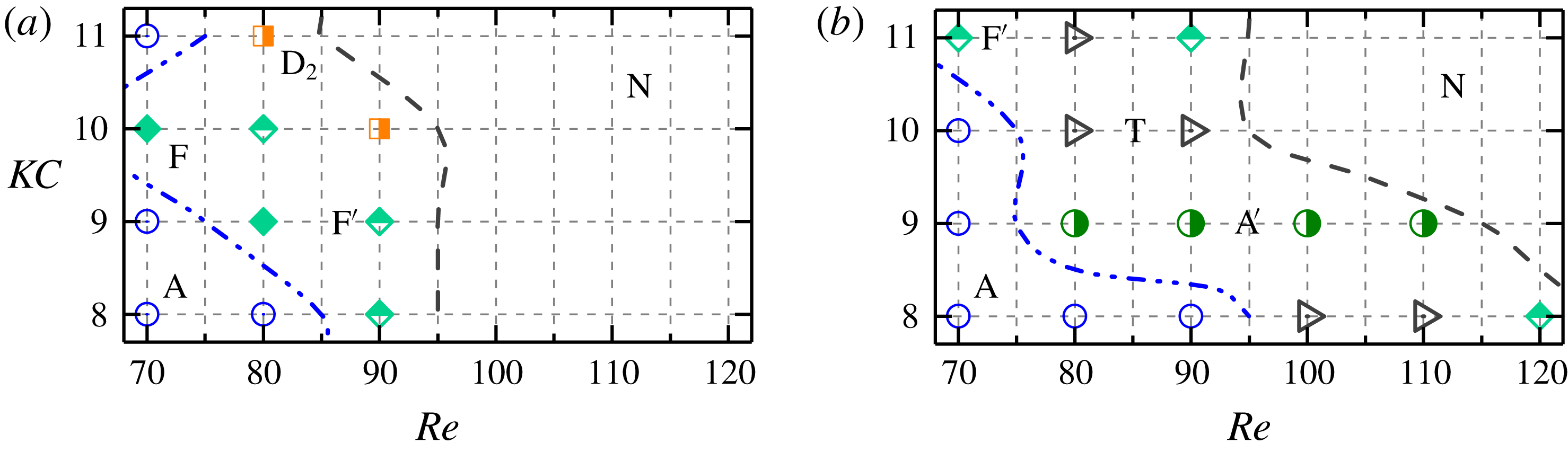
Classification of flow regimes of oscillatory flow around four cylinders in the diamond arrangement at different gap ratios. Cases for different regimes are marked with different symbols and colours along with regime names. The prime symbol (
 $\text{}^{\prime }$
) stands for quasi-periodic regimes with half-filled symbols. Cases only hold
 $K_{y}$
symmetry but lost
 $H_{1}$
and
 $H_{2}$
symmetries are marked as solid symbols which are located between blue dot lines and blue dashed dot lines. The black dashed lines are the symmetry-breaking boundaries where the top right regions, marked ‘N’, denote that none of symmetries were found. The cases for stability analysis are marked by yellow areas in (a) and (b).

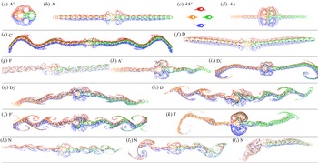
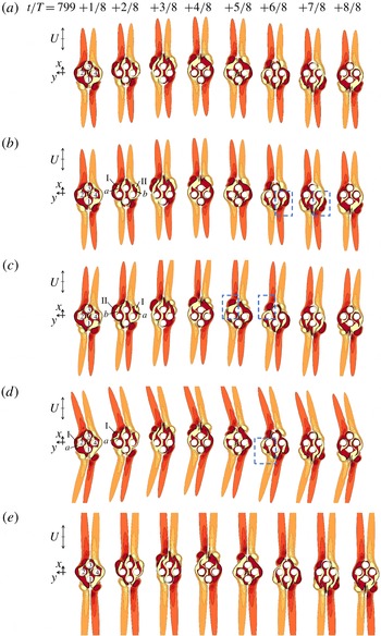
Flow regimes represented by streaklines for oscillatory flow past a cluster of four cylinders in a diamond arrangement at (a) regime
 $\text{A}^{\ast }$
at
 $(G,KC,Re)=(0.5,4,50)$
in 10T; (b) regime A at (1, 9, 130) in 10T; (c) regime
 $4\text{A}^{\ast }$
at (4, 4, 60) in 10T; (d) regime 4A at (4, 12, 50) in 10T; (e) regime
 $\text{C}^{\prime }$
at (1, 11, 110) in 23T; (f) regime D at (1, 12, 110) in 10T; (g) regime F at (0.5, 12, 170) in 10T; (h) regime
 $\text{A}^{\prime }$
at (1, 6, 180) in 10T; (
 $i_{1}$
) regime
 $\text{D}_{1}^{\prime }$
at (2, 11, 80) in 30T; (
 $i_{2}$
) regime
 $\text{D}_{2}^{\prime }$
at (2, 11, 90) in 15T; (
 $i_{3}$
) regime
 $\text{D}_{3}^{\prime }$
at (2, 10, 100) in 15T; (j) regime
 $\text{F}^{\prime }$
at (2, 8, 120) in 20T; (k) regime T at (2, 10, 80) in 20T; (
 $l_{1}$
) regime N at (0.5, 7, 210) in 10T; (
 $l_{2}$
) regime N at (0.5, 8, 200) in 10T and (
 $l_{3}$
) regime N at (1, 12, 120) in 10T. The oscillatory flow is in the horizontal direction. The evolution of the propagation of massless particles for (e, h–k and
 $l_{3}$
) are available as the online supplementary movies ‘Movie 1.mp4–Movie 8.mp4’.

3.1 Regime maps
Detailed maps of flow regimes are shown in figure 4 and the corresponding flow features are illustrated by streaklines in figure 5. The existing names of flow regimes (e.g. regimes
 $\text{A}/\text{A}^{\ast }$
, D and F listed in table 1) from studies on a single cylinder are utilized as much as possible in the classification, especially at small gap ratios where the flow around the cluster is similar to that around a single body (e.g. Tatsuno & Bearman Reference Tatsuno and Bearman1990; Elston et al.
Reference Elston, Blackburn and Sheridan2006; Tong et al.
Reference Tong, Cheng, Zhao, Zhou and Chen2014a
, Reference Tong, Cheng, Zhao and An2015). At relatively large gap ratios where the flow is mainly characterized by features around individual cylinders, combined names of flow regimes of a single cylinder (regimes
 $4\text{A}/4\text{A}^{\ast }$
) are employed. The quasi-periodic flows are denoted by the prime symbol, such as
 $\text{A}^{\prime }$
,
 $\text{C}^{\prime }$
,
 $\text{D}^{\prime }$
and
 $\text{F}^{\prime }$
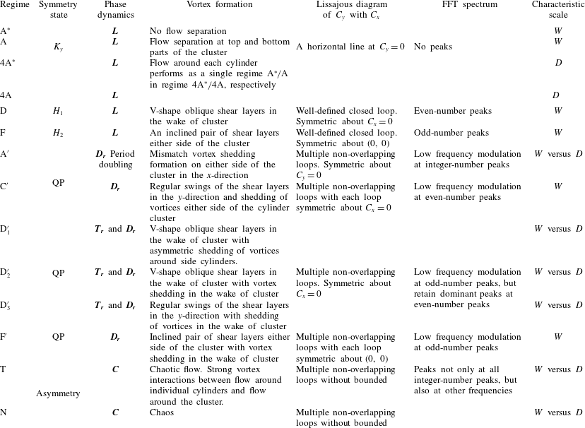
. Regime T denotes a transitional flow state to desynchronized flows and is characterized by aperiodic variations of total lift coefficient. The evolution of the propagation of massless particles for quasi-periodic and desynchronized flows are available as the online supplementary movies ‘Movie 1.mp4–Movie 8.mp4’ at https://doi.org/10.1017/jfm.2019.609. The flow features, force and phase characteristics of different flow regimes are summarized in appendix B. These flow regimes can largely be classified into three groups, namely the synchronous, quasi-periodic and desynchronized flows, which will be discussed in detail in the following sections.
3.2 Synchronous flows
Synchronous flows are defined as those cases where the flow response around the cylinder(s) is synchronized with the incoming oscillatory flow. The characteristics of the synchronous flows include: (i) the Lissajous phase diagram of
 $C_{y}$
with
 $C_{x}$
forms a well-defined closed loop; (ii) the dominant frequency components with sharp peaks in the lift coefficient spectrum appear at the integer multiples of
 $f_{u}T$
; and (iii) one of the symmetry conditions specified in (1.2)–(1.4) are satisfied. The dominant characteristic length scale which influences the formation of synchronous flows gradually transits from the cluster scale W to the cylinder scale D with increasing G. The flow features of synchronous flow regimes are briefly described only because they are similar to those reported in Tong et al. (Reference Tong, Cheng, Zhao and An2015).
3.2.1 Regimes
$\text{A}/\text{A}^{\ast }$
and
$4\text{A}/4\text{A}^{\ast }$


Typical cluster-scale regime
 $\text{A}^{\ast }$
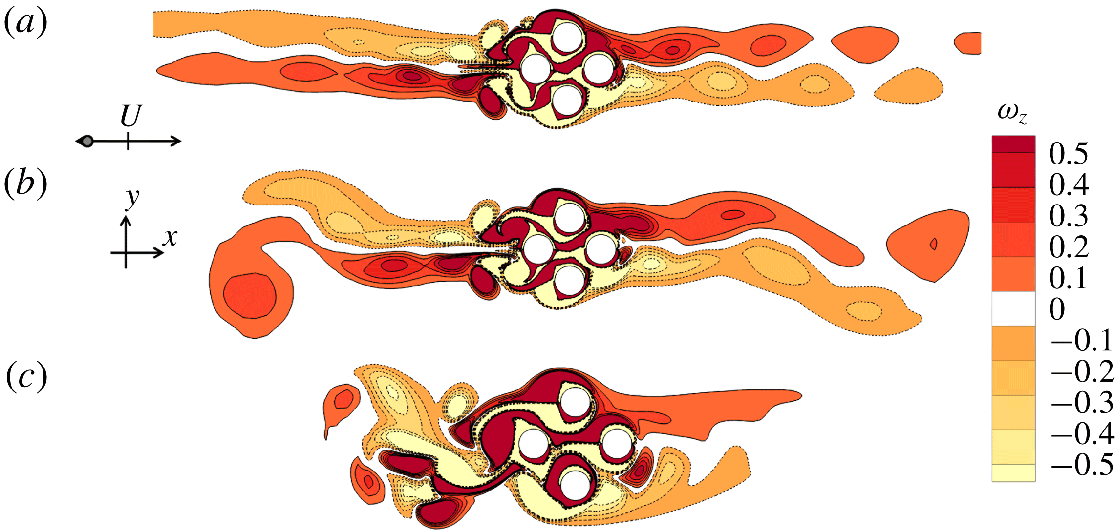
and A flows are shown in figures 6(a) and 6(b), respectively, where vortex shedding is observed in regime A but not in regime A*. To illustrate the similarity between regime A flow around the cluster and that around single cylinder, oscillatory flow around a diamond cylinder with rounding corners is simulated at
 $(KC,Re)=(4.5,130)$
. Despite the differences in flow structures close to the cylinder surfaces, the vorticity contours in the far wake are similar in the two configurations (figure 6
b,c). Regime
 $\text{A}/\text{A}^{\ast }$
occupies a large area in the KC–Re plane at small gap ratios (e.g.
 $G=0.5$
and 1 where the cluster is more like a single body) but only a small area at
 $G=2$
and none at
 $G=4$
(figure 4).
Flow characteristics represented by vorticity contours for six
 $K_{y}$
symmetry cases at: (a) regime
 $\text{A}^{\ast }$
at
 $(G,KC,Re)=(0.5,4,50)$
; (b) regime A at (1, 9, 130); (c) regime A flow for a single diamond cylinder with rounding corners at
 $(KC,Re)=(4.5,130)$
; (d) regime
 $4\text{A}^{\ast }$
at (4, 4, 60); (e) regime 4A at (4, 12, 50) and (f) regime 4A at (2, 4, 190). Two instantaneous contours of vorticity contours between
 $\unicode[STIX]{x1D714}_{z}=-0.5$
and
 $+0.5$
with cutoff level
 $\pm$
0.1, where the sampling phase is indicated by a


Regime
 $4\text{A}^{\ast }$
and 4A flows are named based on flow features around each individual cylinder at large gap ratios. Regime
 $4\text{A}^{\ast }$
flow is only observed at small KC values at
 $G=2$
and 4. This observation is also supported by the streaklines shown in figure 5(c) where mixing of the massless particles (released over 10 flow oscillation periods) is not observed. At
 $G=2$
and 4, regime 4A is one of the dominant regimes in the KC–Re plane. As shown in figure 6(e), regime 4A is featured by a regime A flow around each of the in-line cylinders (C1 and C3) and an asymmetric regime A flow around each of the side cylinders (C2 and C4). It is classified as ‘4A’ to avoid too many regime names.
With increasing KC and/or Re, some of the regime 4A flows hold
 $K_{y}$
symmetry but lose
 $H_{1}$
and
 $H_{2}$
symmetry conditions when the flow is on route of transitioning to quasi-periodic or chaotic flows near the boundaries of
 $K_{y}$
symmetry breaking (solid symbols in figure 4). Figure 6(f) shows an example at
 $(G,KC,Re)=(2,4,190)$
where the sizes and strengths of the shear layers on either side of the cluster differ significantly. Similar flow features have previously been reported in oscillatory flow around four cylinders in a square arrangement (Tong et al.
Reference Tong, Cheng, Zhao and An2015).
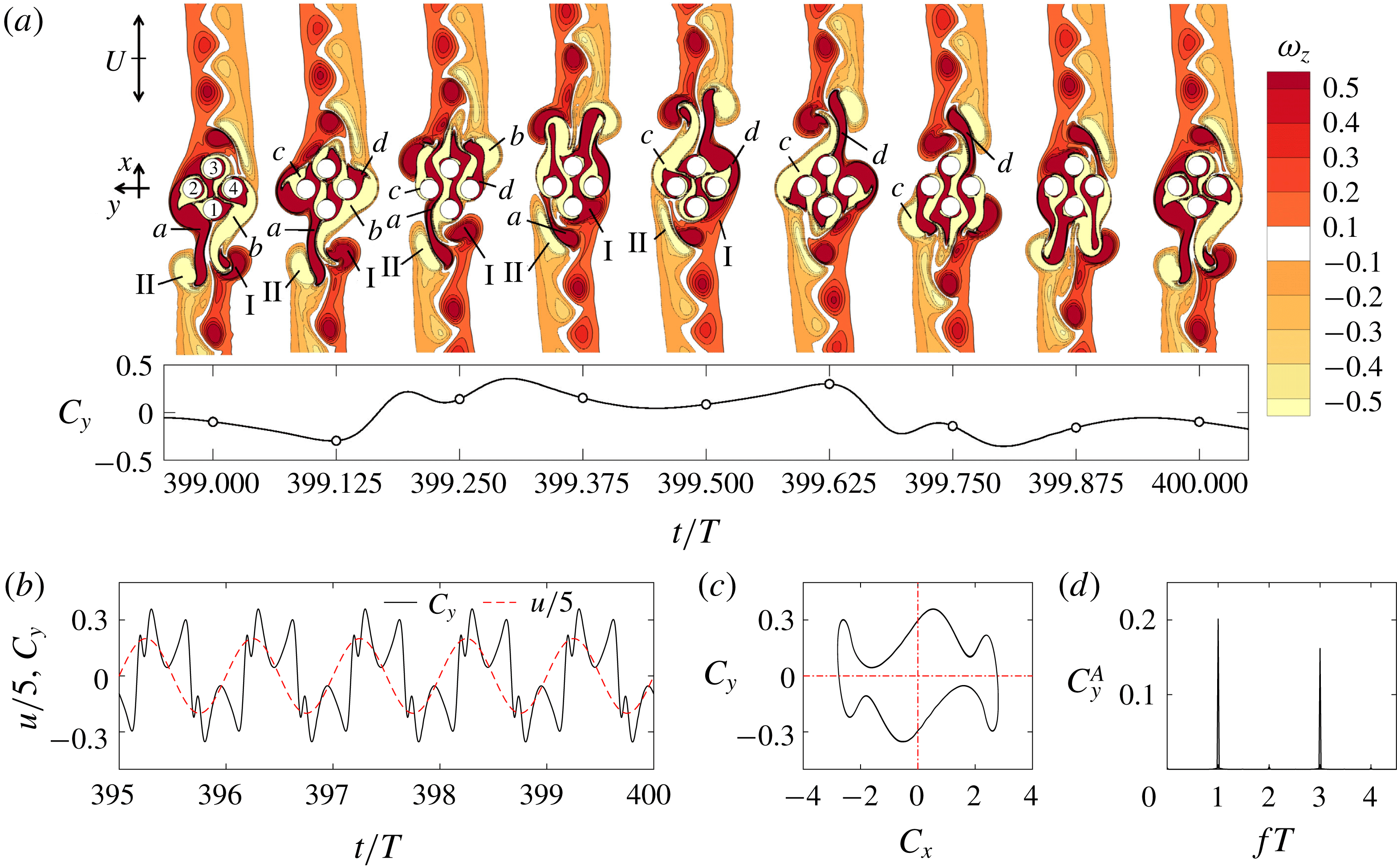
Flow (a) and force (c–d) characteristics of regime F at
 $(G,KC,Re)=(0.5,12,170)$
. (a) Instantaneous vorticity contours at one oscillation period; (b) the time traces of the total lift coefficient (solid black lines) along with the scaled free stream velocity (dashed red lines); (c) the Lissajous phase diagram of
 $C_{y}$
with
 $C_{x}$
; and (d) fast Fourier transform (FFT) spectrum of the total lift coefficient.

3.2.2 Regimes D and F
Regime D and F flows lose
 $K_{y}$
symmetry and are named based on the cluster-scale flow features. The formation of these flows is induced by the interaction of flows around the individual cylinders as well as the cylinder cluster as a single body.
Regime F flow is characterized by an inclined pair of stable shear layers of different signs either side of the cluster relative to the flow oscillation direction (figures 5
g and 7
a). A typical regime F flow observed at
 $(G,KC,Re)=(0.5,12,170)$
in figure 5(g) is similar to that of the regime F flow of a single circular cylinder (figure 2). As shown in figure 7(a), a pair of positive and negative vortices, vortices I and II, interact with the shear layers a and b (also formed from the previous period around the cylinder cluster) of opposite signs, respectively, at
 $t=(399+1/8)T$
. As the flow further advances to the top, vortex a is shed from the cylinder cluster, attracting vortex II to stay on the bottom side of the cluster and eventually merges with the shear layer of the same sign on the bottom of the cluster at
 $+(4/8)T$
. During the same half of the period, vortex I is convected back to the cluster almost freely and enhances the shear layers of the same sign formed at the right side of C4 and C1 at
 $+(3/8)T$
. Due to the different interaction processes of II and a from I and b at the beginning of the oscillation period, the newly formed shear layers of c and d around the cluster have different strengths that lead to the inclination of the vortex street at the top of the cylinder cluster. As the flow reverses, the interaction processes at the left and right sides of the cluster as described above repeat exactly but with the sides swapped, resulting in the
 $H_{2}$
symmetry of the overall flow structure. The interaction of the shear layers formed around C1 and C3 with those formed around the cylinder cluster plays a significant role in forming the regime F flow structure around the cluster, which is different from the regime F flow for a single cylinder. For regime F flows,
 $C_{y}$
changes its sign each half-cycle of flow oscillation due to the diagonal shedding of vortices. The Lissajous phase diagram is symmetric about (0, 0) (figure 7
c), suggesting the flow holds
 $H_{2}$
symmetry (table 2).
Comparisons of the variations of (a) r.m.s. lift coefficients and (b) r.m.s. in-line coefficients on the cylinder cluster and individual cylinders over a range of
 $Re=100$
–230 at
 $(G,KC)=(1,6)$
.

Same as figure 7 but for a typical regime D flow at
 $(G,KC,Re)=(1,12,110)$
.

Most of the regime F flow occupies an area with KC ranging from 5 to 8 and Re between 150 and 230 at
 $G=1$
and several locations at
 $G=0.5$
. The present regime F flow is largely originated from regime A flow with increasing Re, through the loss of
 $H_{1}$
and
 $H_{2}$
symmetries (the filled blue circle in figure 4
b) and then the loss of
 $K_{y}$
symmetry through regime
 $\text{A}^{\prime }$
flows. The influence of vortex shedding around the cylinder cluster on the formation of regime F flow is further illustrated by examining the force coefficients on the cylinder cluster and individual cylinders over a range of Re at
 $(G,KC,Re)=(1,6,100{-}230)$
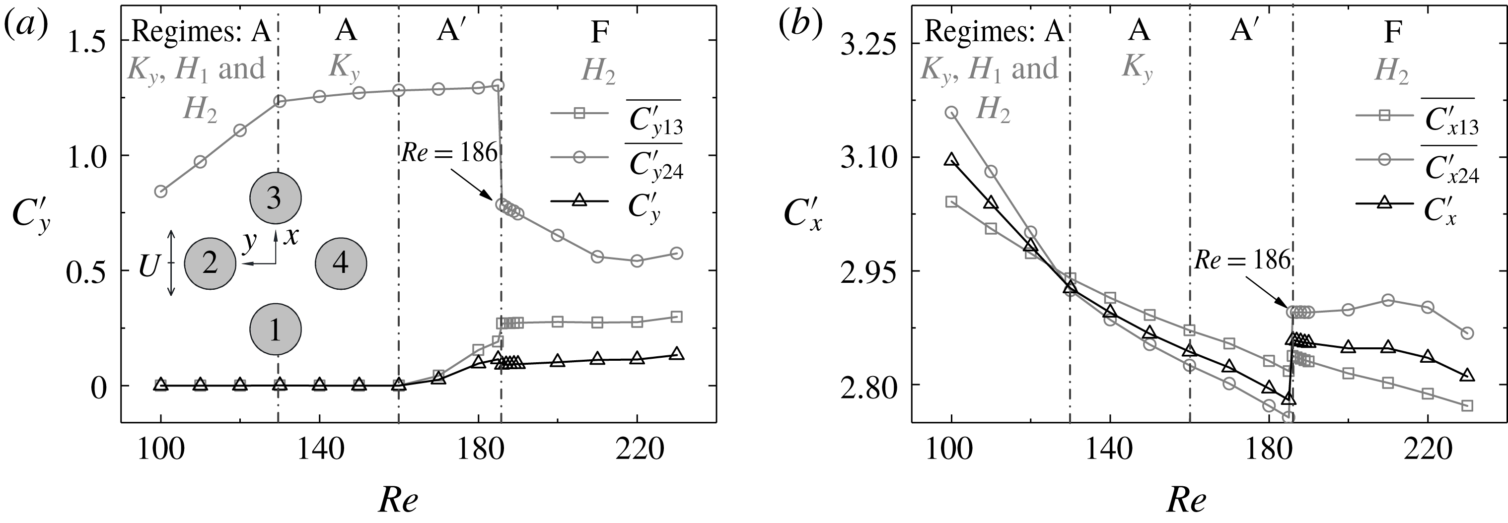
in figure 8. The sudden changes of the r.m.s.
 $\overline{C_{x24}^{\prime }}$
and
 $\overline{C_{y24}^{\prime }}$
, observed at the flow transition to regime F, are clear indications of the interaction of flows around individual cylinders and around the cluster as a whole. The significant reduction of
 $\overline{C_{y24}^{\prime }}$
at the onset of regime F is due to the weakening of the shear layers on the right-hand side of C2 and left-hand side of C4 in figure 8(a), induced by the slight inclinations of vortex shedding direction in regime F.
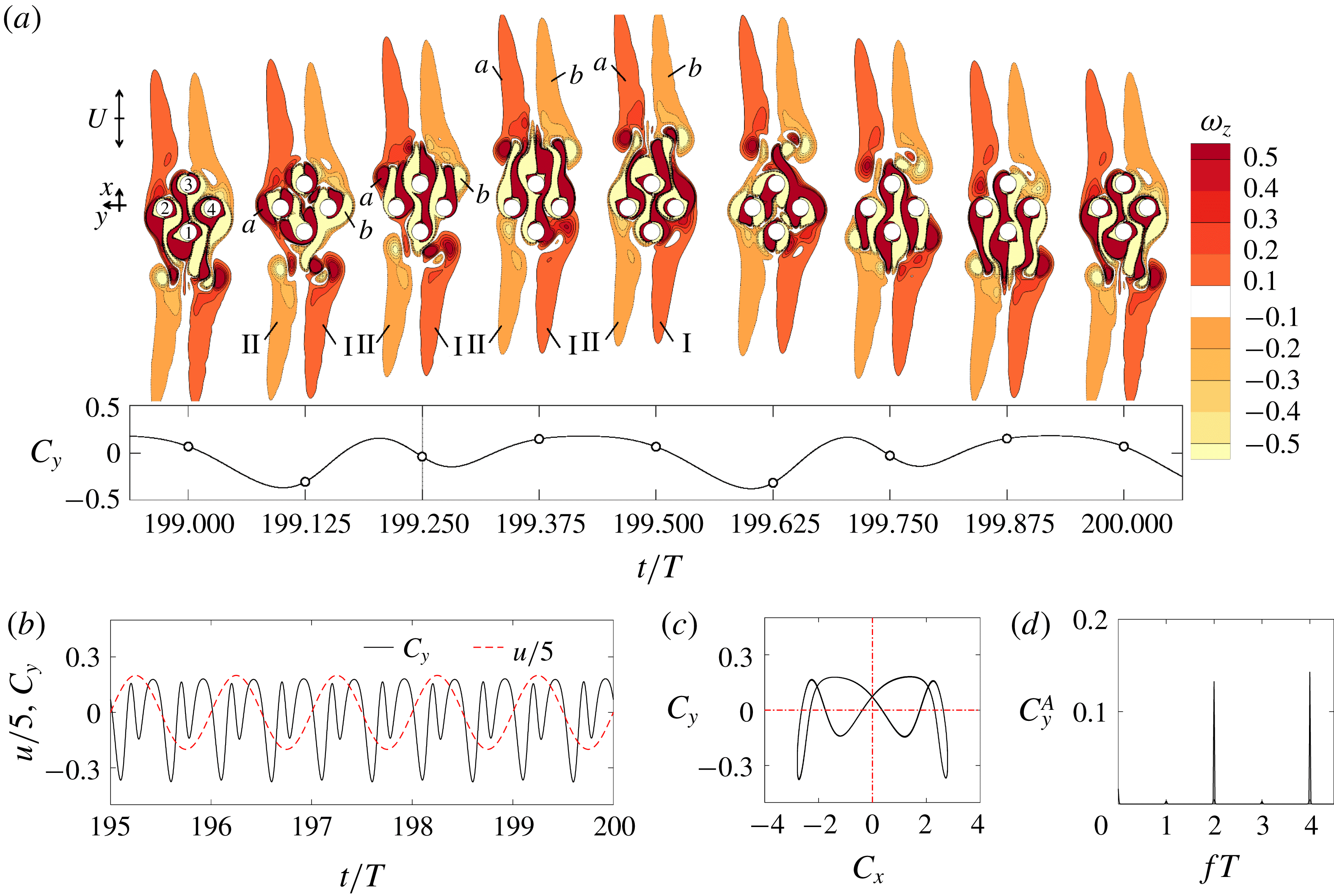
The regime D flow in figure 5(f) and figure 9(a) is characterized by a stable pair of shear layers either side of the cylinder cluster forming V-shape shear layers, in the same manner as regime D of the circular and square cylinders (Tatsuno & Bearman Reference Tatsuno and Bearman1990; Elston et al. Reference Elston, Blackburn and Sheridan2006; Tong et al. Reference Tong, Cheng, Xiong, Draper, An and Lou2017). The formation of the present regime D flow is believed to be a characteristic of flow around the cluster-scale structure, based on the detailed flow field to be presented below and the fact that regime D flow is also formed around solid circular and square cylinders (Tatsuno & Bearman Reference Tatsuno and Bearman1990; Elston et al. Reference Elston, Blackburn and Sheridan2006; Tong et al. Reference Tong, Cheng, Xiong, Draper, An and Lou2017). The V-shape is formed by the shedding of different-sized vortices from either side of the cluster in each half-oscillation period.
The formation mechanism is explored through examining the detailed flow fields sampled at an interval of
 $T/8$
over one period of flow oscillation in figure 9. As the flow accelerates towards the top at
 $t=(199+1/8)T$
, the vortices I and II interact with vortices b and a correspondingly. The interaction between II and a appears to be stronger than that between I and b, leading to a weaker and slower II than I. When I and II are swept back to the cylinder cluster at
 $+(3/8)T$
, vortex I enhances the positive shear layers at the right sides of C1 and C4 more than vortex II does to the negative shear layers at the left sides of C1 and C2, leading to asymmetric shear layers at the left and right sides of C1 and C3, and C2 and C4. The same process repeats again in the next half of the flow period,
 $+(5/8)T$
–
 $+(8/8)T$
, as the flow reverses with vortices of the opposite signs to those involved in the first half of the flow period. The temporal variations of the lift in each half of the period are identical and the mean value is negative as a result of the flow formation. The Lissajous phase diagram of
 $C_{y}$
with
 $C_{x}$
shown in figure 9(c) is symmetric about
 $C_{x}=0$
, suggesting the flow holds
 $H_{1}$
symmetry (table 2).
The present regime D flows are only observed at intermediate gap ratios (e.g.
 $G=1$
and 2) when
 $KC>11$
, but not at
 $G=0.5$
(except the five discrete points within the holes at
 $KC=7$
–8) and
 $G=4$
. The above observed behaviours of regime D flow can be interpreted by the strength of the cluster-scale flow around the cylinders. At very small gap ratios such as
 $G=0.5$
, the cluster-scale flow dominates due to the large blockage effect of the cluster. The flow around the cluster is similar to flow around a single solid cylinder. If the projected width
 $W=3.12D$
of the cluster is used to define the cluster-scale
 $KC_{w}$
, the corresponding
 $KC_{w}$
for the cluster will be reduced by 3.12 times of their counterparts normalized using D, leading to a maximum
 $KC_{w}<4$
covered in the present study. No regime D flow occurs at
 $KC<5$
for a circular cylinder, based on the regime map shown in figure 2. The occurrence of regime D flows at the five discrete points within the holes at
 $KC=7$
–8 and
 $G=0.5$
is an exception and will be explained separately in § 4.1.
As G is increased to 1, the increase of flow rate through the gaps weakens the cluster-scale effect due to the reduction of blockage of the cluster, effectively leading to an increase of cluster-scale
 $KC_{w}$
through the reduction of W. The increase of
 $KC_{w}$
is the cause for the appearance of regime D flow at
 $KC=12$
and
 $G=1$
, because
 $KC_{w}$
is likely larger than 5 which is the minimum KC required for the appearance of regime D for an isolated circular cylinder. At
 $G=2$
, the cluster effect is further weakened, which leads to the appearance of regime D flow at even lower
 $KC(=11)$
than that
 $KC=12$
at
 $G=1$
through the same mechanism explained above. No cluster-scale regime D flow occurs at
 $G=4$
is largely because the cluster-scale effect is rather weak and flows around individual cylinders dominate the flow response at this gap ratio. The interactions of flows around individual cylinder are attributed to the absence of regime D flows.
The areas occupied by the regime D flows in the regime maps for the diamond arrangement of the cylinders investigated in the present study are much smaller than its counterparts in the square arrangement of the cylinders reported by Tong et al. (Reference Tong, Cheng, Zhao and An2015). Regime D flow was only observed at
 $G=0.5$
for the square arrangement (Tong et al.
Reference Tong, Cheng, Zhao and An2015). The cause for the above observations is that the blockage effect of the cluster in the diamond arrangement of the cylinders is stronger than its counterpart in the square arrangement of the cylinders, leading to a larger
 $KC_{w}$
in the former than the latter at identical G values.
The sharp peaks of
 $C_{y}$
spectrum appear at even-number peaks of
 $f_{u}T$
in figure 9(d) for regime D flows and at odd-number peaks of
 $f_{u}T$
in figure 7(d) for regime F flows, due to their symmetry states as detailed in table 2. For instance, the dominant frequency peak appears at
 $fT=4$
in figure 9(d) simply because
 $C_{y}(t)$
has four peaks in T (equivalently two peaks in 0.5T). One of the two peaks in 0.5T is induced by the detachment of newly generated vortices (e.g. a and b at around
 $t=(199+2/8)T$
in figure 9
a) and the other is due to the shed vortex when it is swept back to the cylinder cluster (e.g. I and II at around
 $t=(199+3/8)T$
in figure 9
a).
3.3 Quasi-periodic flows
Four types of quasi-periodic flows, namely
 $\text{A}^{\prime }$
,
 $\text{C}^{\prime }$
,
 $\text{D}^{\prime }$
and
 $\text{F}^{\prime }$
, are identified and each of them holds a well-defined secondary period. The local flow features are similar to those in corresponding synchronous regimes of A, C, D and F. Both of the characteristic length scales of D and W are important for the development of the quasi-periodic flows and the physics behind those features are explained below.
3.3.1 Regime
$\text{F}^{\prime }$

Regime
 $\text{F}^{\prime }$
is observed in the range of
 $KC=6$
–10 at
 $G=2$
and
 $KC=7$
–12 at
 $G=4$
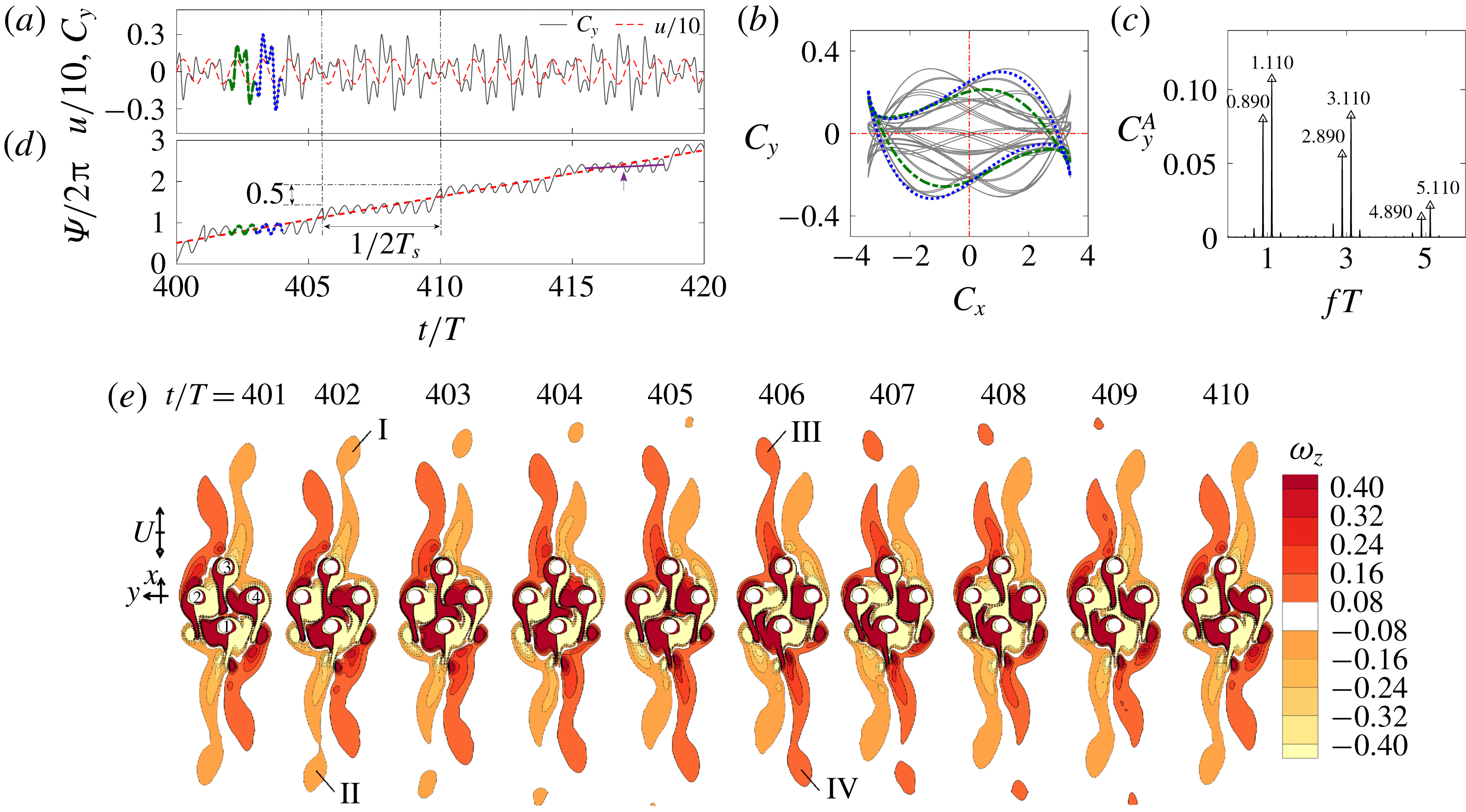
. Figure 10 shows the characteristics of a typical regime
 $\text{F}^{\prime }$
at
 $(G,KC,Re)=(2,8,120)$
. The evolution of the streaklines for the regime
 $\text{F}^{\prime }$
flow in 20T is available in the online supplementary movie ‘Movie 1.mp4’. The quasi-periodic feature can be observed from the temporal variation of
 $C_{y}$
in figure 10(a) where
 $C_{y}$
has a feature that repeats approximately 9T, in addition to the oscillation cycles with the period T. The Lissajous diagram is approximately symmetric about
 $(C_{x},C_{y})=(0,0)$
in one oscillation period (see the green and blue cycles in figure 10
b), suggesting the flow largely holds
 $H_{2}$
symmetry in a similar manner to the synchronous regime F flow. The occurrence of double sharp peaks around odd-number peaks of
 $f_{u}T$
in figure 10(c) suggests that
 $C_{y}(t)$
has two frequencies, namely the fundamental lift frequency
 $f_{l}T=1$
and the secondary frequency
 $f_{s}T=0.110$
. The fundamental lift frequency is modulated by
 $f_{s}T=0.110$
(or with a period of
 $T_{s}\approx 9.091T$
) and its higher-order harmonics.
Force (a–d) and flow (e) characteristics of a typical regime
 $\text{F}^{\prime }$
flow at
 $(G,KC,Re)=(2,8,120)$
. (a) Time traces of the total lift coefficient (the dark grey solid line) along with the scaled free-stream velocity (the red dashed line); (b) Lissajous phase diagram of
 $C_{y}$
with
 $C_{x}$
; (c) FFT spectrum of
 $C_{y}$
; (d) time traces of
 $\unicode[STIX]{x1D6F9}(t)$
and (e) vorticity contours at the selected instants, when the inlet velocity is about to change to the positive x direction. The green dash dot line and blue dot line in (a), (b) and (d) are the signals from 403rd and 404th cycles of the flow oscillation, respectively.

The temporal variation of
 $\unicode[STIX]{x1D6F9}$
revealed by figure 10(d) is similar to that of point 3 in figure 3(a), which involves both phase drifting and slipping. In this case
 $\unicode[STIX]{x1D6F9}(t)$
drifts upwards slowly between two
 $T_{s}/2$
, followed by a sudden slip. Since the response frequency
 $f_{y}T$
appears near
 $fT=1,f_{l}T$
is taken as 1 in (2.9). The mean slope of
 $\overline{\unicode[STIX]{x1D6F9}_{T_{a}}}/2\unicode[STIX]{x03C0}$
with
 $T_{a}=T_{s}$
(the red dashed line in figure 10
d) is 0.11, which is identical to the secondary frequency of
 $f_{s}T$
observed in figure 10(c). The slow upwards drift of
 $\unicode[STIX]{x1D6F9}(t)$
over
 $T_{s}/2$
(at a rate of approximately
 $\overline{\dot{\unicode[STIX]{x1D6F9}}_{T_{a}}}/2\unicode[STIX]{x03C0}=0.026$
), illustrated by the slope of the purple solid line in figure 10(d), suggests that the flow features associated with the secondary frequency are largely synchronized with the incoming flow (external forcing).
The flow mechanisms associated with the phase dynamics observed above are examined by taking a stroboscopic view of vorticity contours of the flow at a fixed phase angle in each T over
 $T_{s}$
, as shown in figure 10(e). The vorticity patterns repeat approximately every 9T, consistent with
 $T_{s}\approx 9.091T$
obtained from the FFT analysis. The low frequency component
 $f_{s}T=0.110$
is associated with the secondary flow feature where the shear layers in the wake of the cylinder cluster become unstable and two vortex pairs (I and II and III and IV) are shed from the far tips of the shear layers in each
 $T_{s}$
, in contrast to the stable formation observed in figure 7. For instance, the geometry and strength of the long shear layers either side of the cylinder cluster undergo periodic changes that are alternated with a spatio-temporal
 $H_{2}$
symmetry, which is consistent with the slow and incremental change of flow structures inferred from the phase dynamics discussed above. During the incremental change process, two negative vortices, namely I and II shown in figure 10(e), are shed simultaneously from the far tips of the shear layers either side of the cylinder cluster at around
 $t/T=402$
, followed by the shedding of two positive vortices (III and IV) after approximately half of
 $T_{s}$
at around
 $t/T=406$
. The timings of the vortex shedding, e.g. vortex I and II, and III and IV at
 $t/T=402$
and 406, are quite close to the moments of the phase slips at around
 $t/T=401$
and 405 in figure 10(d) correspondingly. The phase slip at the end of each
 $T_{s}/2$
is believed to be associated with a sudden adjustment of the flow structure on one side of the cylinder cluster (
 $x$
direction) in
 $T_{s}/2$
. The total phase slip over
 $T_{s}$
is
 $2\unicode[STIX]{x03C0}$
.
The total slip (or jump) of
 $\unicode[STIX]{x03C0}$
for each half
 $T_{s}$
is explained with reference to the circle map defined by (2.12). By assuming a very small
 $\unicode[STIX]{x1D700}\approx 0$
, we get
 $$\begin{eqnarray}\displaystyle \unicode[STIX]{x1D719}_{s}^{N+1}\approx \unicode[STIX]{x1D719}_{s}^{N}+2\unicode[STIX]{x03C0}T/T_{s}. & & \displaystyle\end{eqnarray}$$
In this case,
 $T/T_{s}\approx 1/9.091$
with the fundamental lift frequency
 $f_{l}T=1$
. By taking into account the above observations in (3.1), we get
 $$\begin{eqnarray}\displaystyle \unicode[STIX]{x1D719}_{s}^{N+1}\approx \unicode[STIX]{x1D719}_{s}^{N}+2\unicode[STIX]{x03C0}/9.091. & & \displaystyle\end{eqnarray}$$
With reference to a fixed
 $t_{0}$
of the external forcing,
 $\unicode[STIX]{x1D719}_{s}^{N+1}$
experiences an incremental change of
 $2\unicode[STIX]{x03C0}/9.091$
in each T. This incremental change is accumulated from one period to the next until the accumulation reaches
 $2\unicode[STIX]{x03C0}$
at the end of the secondary period of
 $T_{s}$
, when a new incremental change and accumulation cycle starts over from there again. Figure 10(d) shows that the actual incremental change rate of
 $\unicode[STIX]{x1D6F9}(t)$
over each epoch of
 $t<T_{s}/2$
is much smaller than the average rate of
 $2\unicode[STIX]{x03C0}/9.091$
. This mismatch of the change rates of
 $\unicode[STIX]{x1D6F9}(t)$
leads to the phase slip at the end of each epoch. If we integrate (3.2) over a period of
 $T_{s}/2$
and ignore the small change of
 $\unicode[STIX]{x1D6F9}$
(t) over each epoch, we get a phase slip of
 $\unicode[STIX]{x03C0}$
at
 $t_{0}+T_{s}/2$
. Another phase slip of
 $\unicode[STIX]{x03C0}$
is expected in the next
 $T_{s}/2$
, leading to a total phase slip of
 $2\unicode[STIX]{x03C0}$
over one
 $T_{s}$
. Physically each phase slip corresponds to the shedding of vortices from tips of the shear layers in figure 10(e), enabling the phase of slow secondary flow features to catch up with the phase of fast flow oscillation. The total phase slip of
 $2\unicode[STIX]{x03C0}$
over one
 $T_{s}$
in this case is because
 $T/T_{s}$
is very close to a rational number and the fundamental lift frequency
 $f_{l}T=1$
. It will be shown later on that the phase slip in one
 $T_{s}$
is not necessarily
 $2\unicode[STIX]{x03C0}$
, depending on the ratio of
 $T_{l}/T_{s}$
.
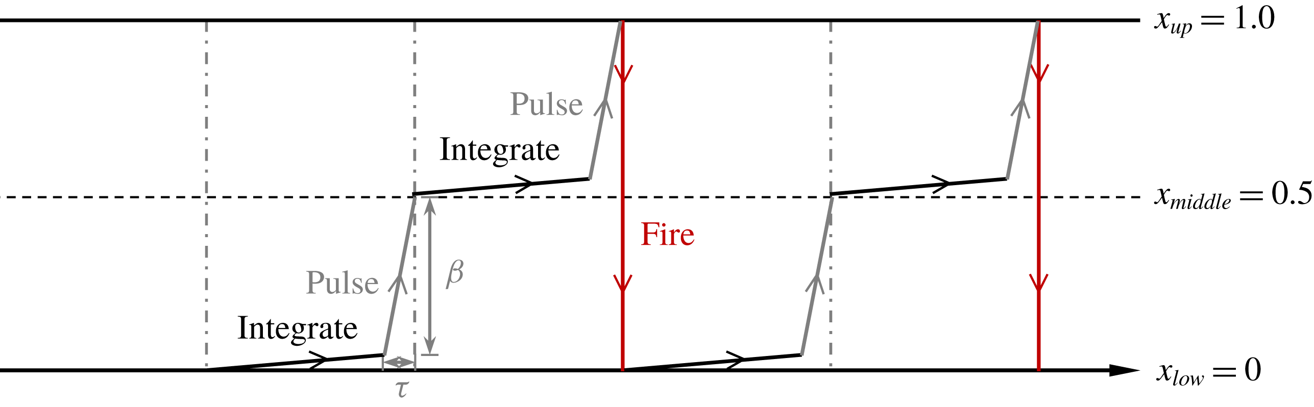
Sketch of the integrate-and-fire oscillator in regime
 $\text{F}^{\prime }$
.

Secondary frequency of the total lift coefficients at (a)
 $(G,KC,Re)=(2,7,120{-}140)$
and (b)
 $(G,KC,Re)=(4,10{-}12,70)$
.

The phase dynamics observed in this case is actually very similar to the behaviour of a relaxation (integrate-and-fire) self-sustained oscillator with periodic pulses, as described in Pikovsky et al. (Reference Pikovsky, Rosenblum and Kurths2003, p. 202). The present integrate-and-fire oscillator is described by one scalar variable x which represents the secondary flow process. The dynamics of
 $x(t)$
in regime
 $\text{F}^{\prime }$
are comprised of four processes as illustrated in figure 11: (i) integration process where x grows linearly in time
 $x=(t-t_{n})/T_{s}$
with
 $t_{n}$
the moment of the previous firing; (ii) the oscillator then is affected by another oscillator, which forms a pulse (or a rapid growth) on x in a short time duration
 $\unicode[STIX]{x1D70F}$
and x reaches 0.5 after the pulse; (iii) the second integration and pulse processes continue in the next time
 $x(t)=0.5$
to 1.0; and (iv) firing when x reaches the threshold
 $x_{up}=1.0$
and the value of x is reset to
 $x_{low}=0$
instantly. The integration process described above corresponds to the incremental change of the secondary flow and the pulse corresponds to the shedding of vortices from the shear layers of either side of the cylinder cluster that affect the integrate-and-fire oscillator in a similar manner of periodic pulse in a period of
 $T_{s}/2$
. If we denote the amplitude of each pulse by
 $\unicode[STIX]{x1D6FD}$
, two scenarios are possible: (i) if
 $x(t)+\unicode[STIX]{x1D6FD}<x_{up}$
, the integration process continues and (ii) if
 $x(t)+\unicode[STIX]{x1D6FD}>x_{up}$
, the oscillator fires. In the regime
 $\text{F}^{\prime }$
flow examined here, we have the scenarios (i) at each
 $t_{n}+T_{s}/2$
and (ii) at each
 $t_{n}+T_{s}$
.
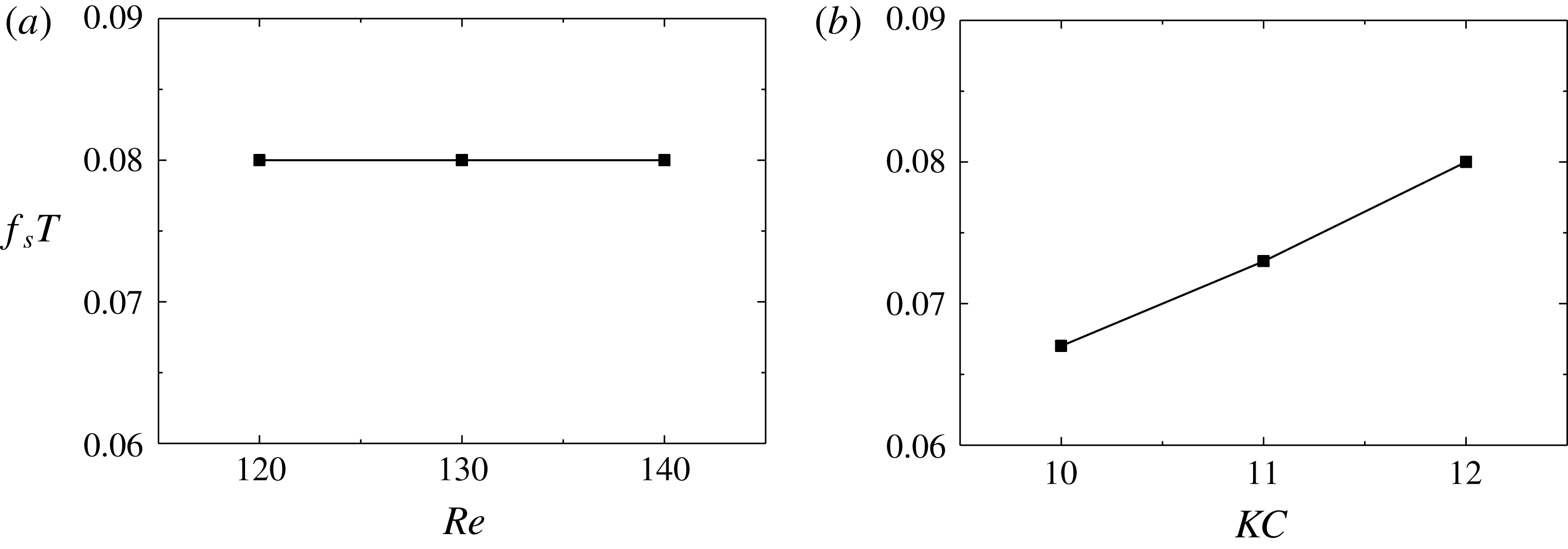
The influence of Re and KC on the secondary frequency
 $f_{s}T$
in regime
 $\text{F}^{\prime }$
flows is examined in figure 12, where Re varies from 120 to 140 at
 $KC=7$
and
 $G=2$
in (a) and KC varies from 10 to 12 at
 $Re=70$
and
 $G=4$
in (b). The secondary frequency is insensitive to the variation of Re at the fixed
 $KC=7$
(e.g.
 $f_{s}T=0.08$
in figure 12
a) but increases with increasing KC in figure 12(b). Tong et al. (Reference Tong, Cheng, Xiong, Draper, An and Lou2017) also found that the secondary frequency in regime
 $\text{F}^{\prime }$
is sensitive to the variation of KC in oscillatory flow around a square cylinder.
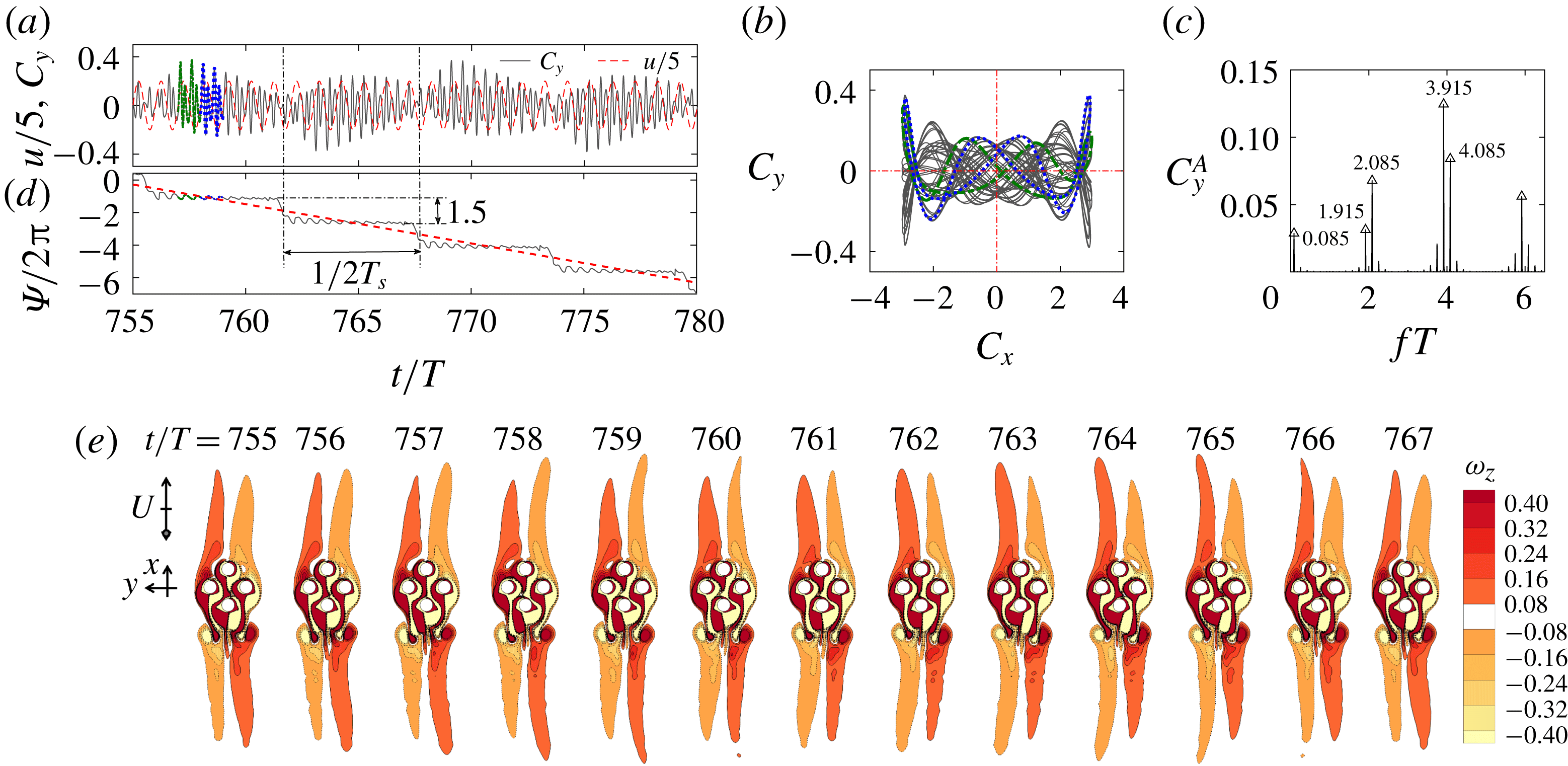
Same as figure 10 but in regime
 $\text{C}^{\prime }$
at
 $(G,KC,Re)=(1,11,110)$
. The green dash dot line and blue dot line in (a), (b) and (d) are the signals from 757th and 758th cycles of flow oscillation, respectively.

3.3.2 Regime
$\text{C}^{\prime }$

Most of the regime
 $\text{C}^{\prime }$
flows are observed for
 $G=1$
and
 $KC\geqslant 10$
, where, at the cluster scale, the flow is similar to the synchronous regime C flow around an isolated cylinder (e.g. Tatsuno & Bearman Reference Tatsuno and Bearman1990; Elston et al.
Reference Elston, Blackburn and Sheridan2006; Tong et al.
Reference Tong, Cheng, Xiong, Draper, An and Lou2017; Xiong et al.
Reference Xiong, Cheng, Tong and An2018b
). A new name
 $\text{C}^{\prime }$
is used to be consistent with the definition of other quasi-periodic regimes in the present study.
A typical regime
 $\text{C}^{\prime }$
flow is illustrated in figure 5(e) and figure 13 at
 $(G,KC,Re)=(1,11,110)$
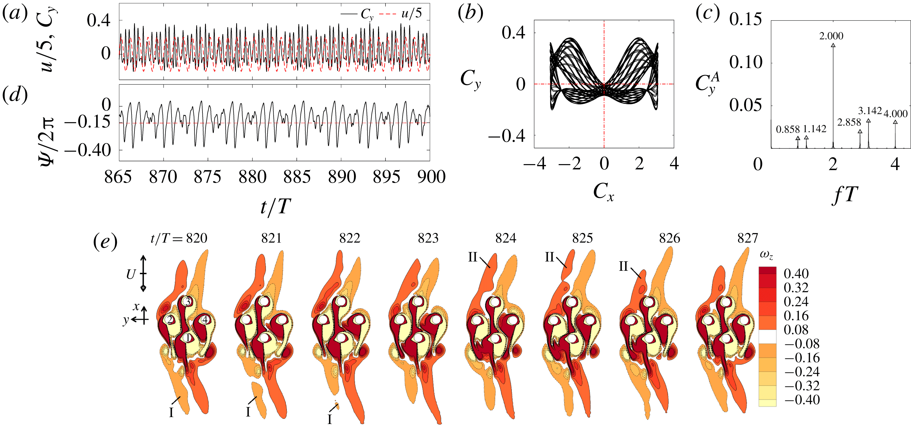
, specifically through the quasi-periodic feature in the temporal variation of
 $C_{y}$
. The evolution of the streaklines for the regime
 $\text{C}^{\prime }$
flow in 20T is available in online supplementary movie ‘Movie 2.mp4’. The Lissajous diagram in a single flow period is symmetric about
 $C_{x}=0$
(figure 13
b), suggesting the flow around the cluster holds the
 $H_{1}$
symmetry (table 2). A low, well-defined frequency component of
 $f_{s}T=0.085$
(or
 $T_{s}\approx 11.765T$
) that modulates even-number peaks of
 $f_{u}T$
is observed in figure 13(c). The low frequency component of
 $f_{s}T=0.085$
is associated with the regular swings of the shear layers in the y-direction and shedding of vortices either side of the cylinder cluster through the stroboscopic snapshots of vorticity contours in figure 13(e). When the shear layer tips swing towards negative direction of y, the mean
 $C_{y}(t)$
is positive in that half
 $T_{s}$
and the process in the next half
 $T_{s}$
is opposite to that of the previous half. The flow features repeat themselves in approximately 12T, consistent with
 $T_{s}\approx 11.765T$
obtained from the FFT analysis. Again the low frequency shear layer instabilities are expected to affect the phase of
 $C_{y}(t)$
, which is quantified by examining phase difference
 $\unicode[STIX]{x1D6F9}(t)$
with
 $f_{l}T=4$
in (2.9). Phase drifting and slipping features are observed again in figure 13(d). The downward trend suggests that the mean frequency of
 $C_{y}(t)$
is smaller than
 $f_{l}$
.
The phase slip of
 $3\unicode[STIX]{x03C0}$
at the end of each
 $T_{s}/2$
is different from the phase slip of
 $\unicode[STIX]{x03C0}$
in the regime
 $\text{F}^{\prime }$
flow shown in figure 10(d) and can be explained based on the circle map represented by (2.13). Since the ratio of
 $T_{s}/T\approx 11.765$
is an irrational number and
 $T_{l}=T/4$
, (2.13) can be written in the following form with
 $\unicode[STIX]{x1D700}\approx 0$
:
 $$\begin{eqnarray}\displaystyle \unicode[STIX]{x1D719}^{N+1}\approx \unicode[STIX]{x1D719}^{N}+\frac{2\unicode[STIX]{x03C0}T_{s}}{T_{l}}\approx \unicode[STIX]{x1D719}^{N}+8\unicode[STIX]{x03C0}(11+0.765)=\unicode[STIX]{x1D719}^{N}+6.120\unicode[STIX]{x03C0}. & & \displaystyle\end{eqnarray}$$
It should be noted that
 $88\unicode[STIX]{x03C0}$
was ignored in (3.3) because
 $\unicode[STIX]{x1D719}^{N+1}$
is a
 $2\unicode[STIX]{x03C0}$
-periodic function over
 $T_{s}$
. A phase jump of approximately
 $6\unicode[STIX]{x03C0}$
over
 $T_{s}$
is suggested by (3.3), leading to a
 $3\unicode[STIX]{x03C0}$
jump over
 $T_{s}/2$
and consistent with the data shown in figure 13(d).
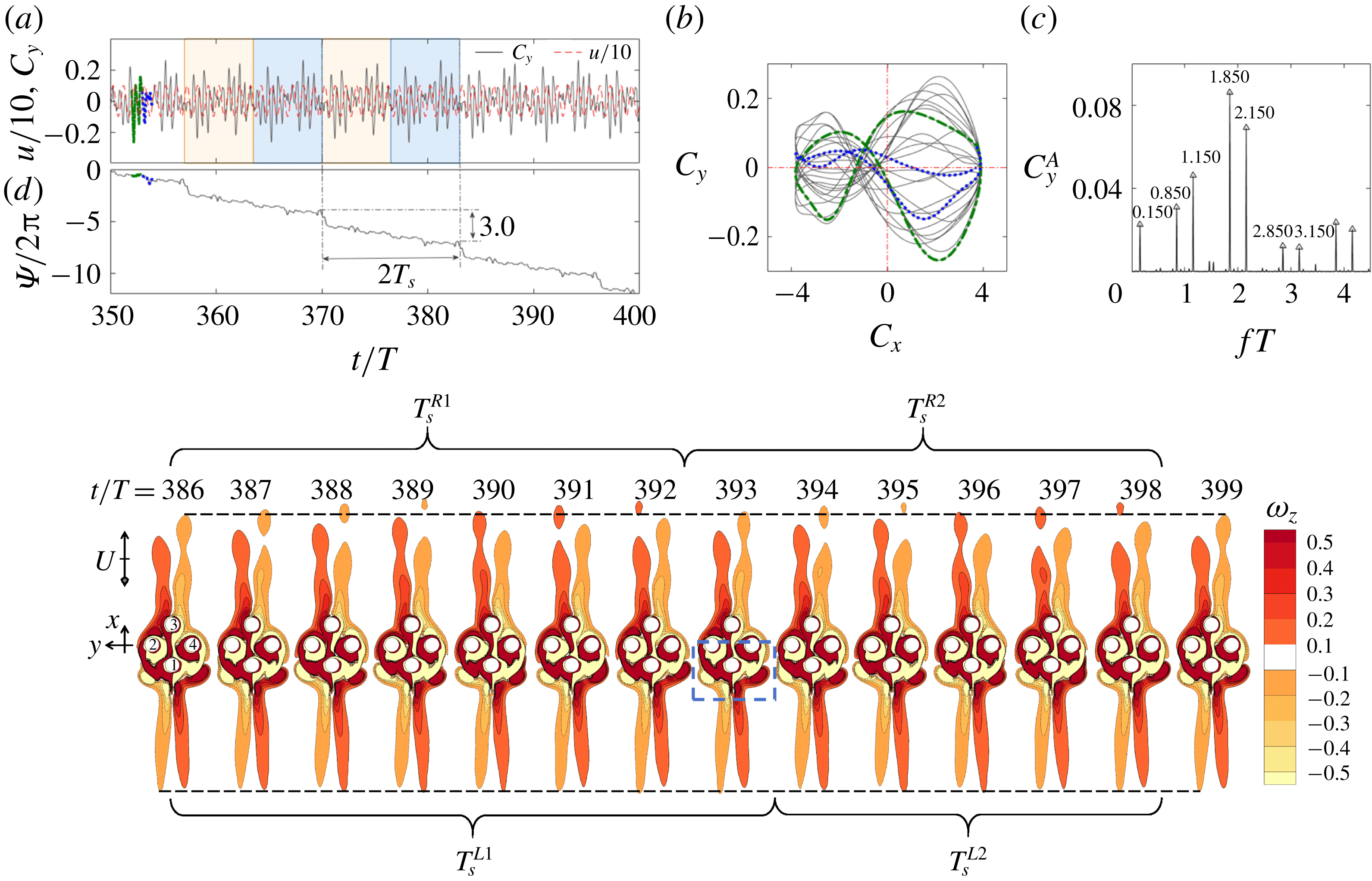
Same as figure 10 but in regime
 $\text{A}^{\prime }$
at
 $(G,KC,Re)=(1,6,180)$
. The green dash dot line and blue dot line in (a), (b) and (d) are the signals from 352th and 353th cycles of flow oscillation, respectively.

3.3.3 Regime
$\text{A}^{\prime }$

Regime
 $\text{A}^{\prime }$
is a new flow regime found in this study and appears at locations between two synchronous regimes A and F at
 $G=1$
, as shown in figure 4(b). A typical regime
 $\text{A}^{\prime }$
flow is illustrated in figure 5(h) and figure 14 at
 $(G,KC,Re)=(1,6,180)$
. The evolution of the streaklines for the regime
 $\text{A}^{\prime }$
flow in 20T is available in online supplementary movie ‘Movie 3.mp4’. The quasi-periodicity of the flow is apparent through the temporal variation of
 $C_{y}$
shown in figure 14(a). The asymmetric feature of the Lissajous diagram in one oscillation cycle shown in figure 14(b) suggests that the flow holds none of the symmetry states listed in (1.2)–(1.4). There are again two frequency components in figure 14(c) with the fundamental lift frequency at
 $f_{l}T=2$
and the secondary frequency at
 $f_{s}T=0.150$
. Since all the symmetry states are broken, modulations by
 $f_{s}T=0.150$
occur at all integer multiples of
 $f_{u}T$
.
Figure 14(a) shows that the temporal variation of
 $C_{y}$
repeats regularly every 13T (the patterns in two coloured blocks), suggesting that the secondary period is approximately 13T. This value does not agree with the value of
 $T_{s}\approx (1/0.150)T=6.667T$
inferred from the power spectrum of
 $C_{y}(t)$
in figure 14(c). To find out the reason for this contradiction, we refer to the stroboscopic snapshots of the vorticity contours within 14T in figure 14(e), which show that: (i) the strength of vortex shedding at the far tips of the shear layers (positive x direction) is different from that in the opposite direction; (ii) the overall flow structure approximately repeats itself in a period of 13T; and (iii) the timings of the vortex shedding cycle from the top shear layers and the oscillation cycle from the bottom side of the cluster differ slightly. For example, the first vortex shedding cycle at the top side, namely
 $T_{s}^{R1}$
, is from
 $t/T=386$
to an instant between
 $t/T=392$
and 393, whereas the first cycle of the oscillation at the bottom side,
 $T_{s}^{L1}$
is from
 $t/T=386$
to an instant between
 $t/T=393$
and 394. The second vortex shedding cycle (
 $T_{s}^{R2}$
) and oscillation cycle (
 $T_{s}^{L2}$
) start at different time instants but finish at the same time instant of
 $t/T=398$
. The observations (ii) and (iii) suggest that the secondary period of the flow is approximately
 $(13/2)T=6.5T$
, which is consistent with the value of
 $T_{s}\approx 6.667T$
inferred from the FFT analysis. The low frequency component of
 $f_{s}T=0.150$
(or
 $T_{s}\approx 6.667T$
) is associated with the regular cluster-scale vortex shedding processes in the wake of cylinder cluster (figure 14
e). The observations (i) and (iii) suggest that the flow structures in the two secondary oscillation (vortex shedding) periods do not match in the phase space, which is consistent with the observation from figure 14(a) that the
 $C_{y}(t)$
patterns in the neighbouring coloured blocks are different.
The phenomenon observed above is similar to the period-doubling behaviour reported in the literature (e.g. Moskalik & Buchler Reference Moskalik and Buchler1990; Papaioannou et al.
Reference Papaioannou, Yue, Triantafyllou and Karniadakis2006), except that the period doubling occurs for the low frequency secondary flow features in the present case. Period doubling occurs as the result of interactions of multiple instabilities in weakly nonlinear systems and is known as one of the routes for transition to chaotic flow (Moskalik & Buchler Reference Moskalik and Buchler1990). Papaioannou et al. (Reference Papaioannou, Yue, Triantafyllou and Karniadakis2006) observed period doubling within the synchronization region for two tandem oscillating cylinders, referring to it as a hole in the synchronization map (similar to the regime
 $\text{A}^{\prime }$
shown in figure 4
b). The multiple flow instabilities that are responsible for the period-doubling regime
 $\text{A}^{\prime }$
in this case include: (i) the local flow instabilities (symmetry breaking) around each cylinder; (ii) vortex shedding at the far tips of the top shear layers; and (iii) the oscillation of the bottom shear layers. The interaction of those flow instabilities is the main reason that regime
 $\text{A}^{\prime }$
occurs between two synchronous regimes A and F. The mismatch of the timings of the shear layer instabilities either side of the cylinder cluster is the cause for the period-doubling behaviour in regime
 $\text{A}^{\prime }$
. The phase dynamics
 $\unicode[STIX]{x1D6F9}(t)$
with
 $f_{l}T=2$
in (2.9) in figure 14(d) is slightly different from those of regimes
 $\text{F}^{\prime }$
and
 $\text{C}^{\prime }$
. Each epoch of downwards drift lasts for approximately
 $2T_{s}\approx 13T$
, followed by a phase slip of approximately
 $6\unicode[STIX]{x03C0}$
. The total phase slip can be explained in the same manner as that offered for the regime
 $\text{C}^{\prime }$
flow.
3.3.4 Regime
$\text{D}^{\prime }$

Regime
 $\text{D}^{\prime }$
flows are mainly found near the boundary of the desynchronized flow zones (regime N) and other quasi-periodic flows at
 $G=1$
and 2 with relatively large KC values (figure 4). Three types of regime
 $\text{D}^{\prime }$
flow, namely
 $\text{D}_{1}^{\prime }$
,
 $\text{D}_{2}^{\prime }$
and
 $\text{D}_{3}^{\prime }$
, are observed in the present study and will be discussed below.
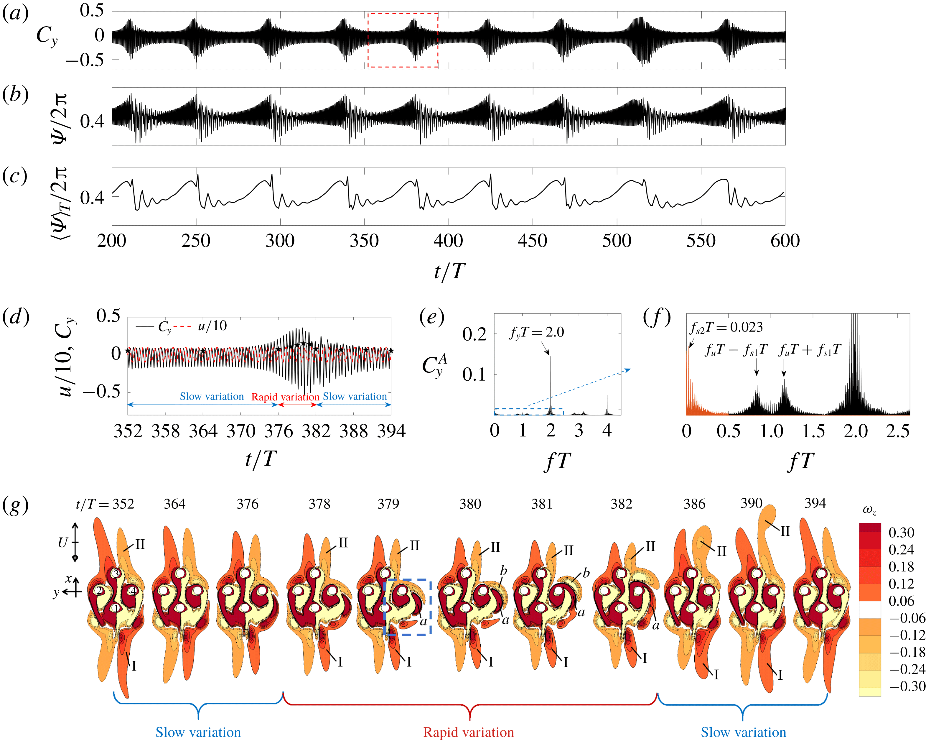
Force (a–f) and flow (g) characteristics of regime
 $\text{D}_{1}^{\prime }$
at
 $(G,KC,Re)=(2,11,80)$
. Time traces of (a) total lift coefficient
 $C_{y}$
, (b) the phase difference
 $\unicode[STIX]{x1D6F9}$
and (c)
 $\overline{\unicode[STIX]{x1D6F9}_{T_{a}}}$
with
 $T_{a}=T$
; (d) a close-up view of
 $C_{y}(t)$
in 43T enclosed by the box in (a); (e) FFT spectrum of
 $C_{y}$
and (f) a close-up view from the box in (e); (g) vorticity contours at chosen instants as indicated by
 $\star$
in (d).

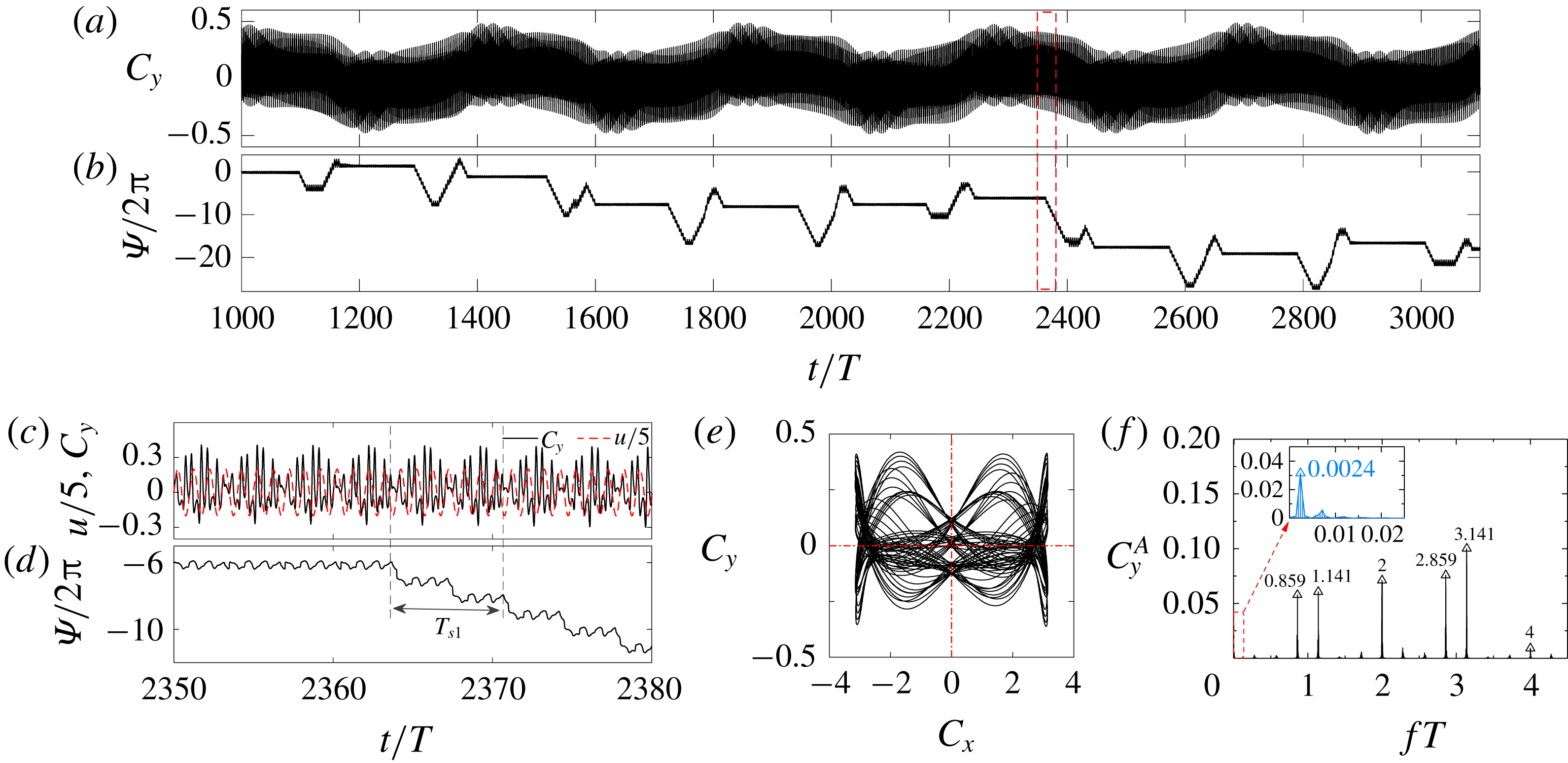
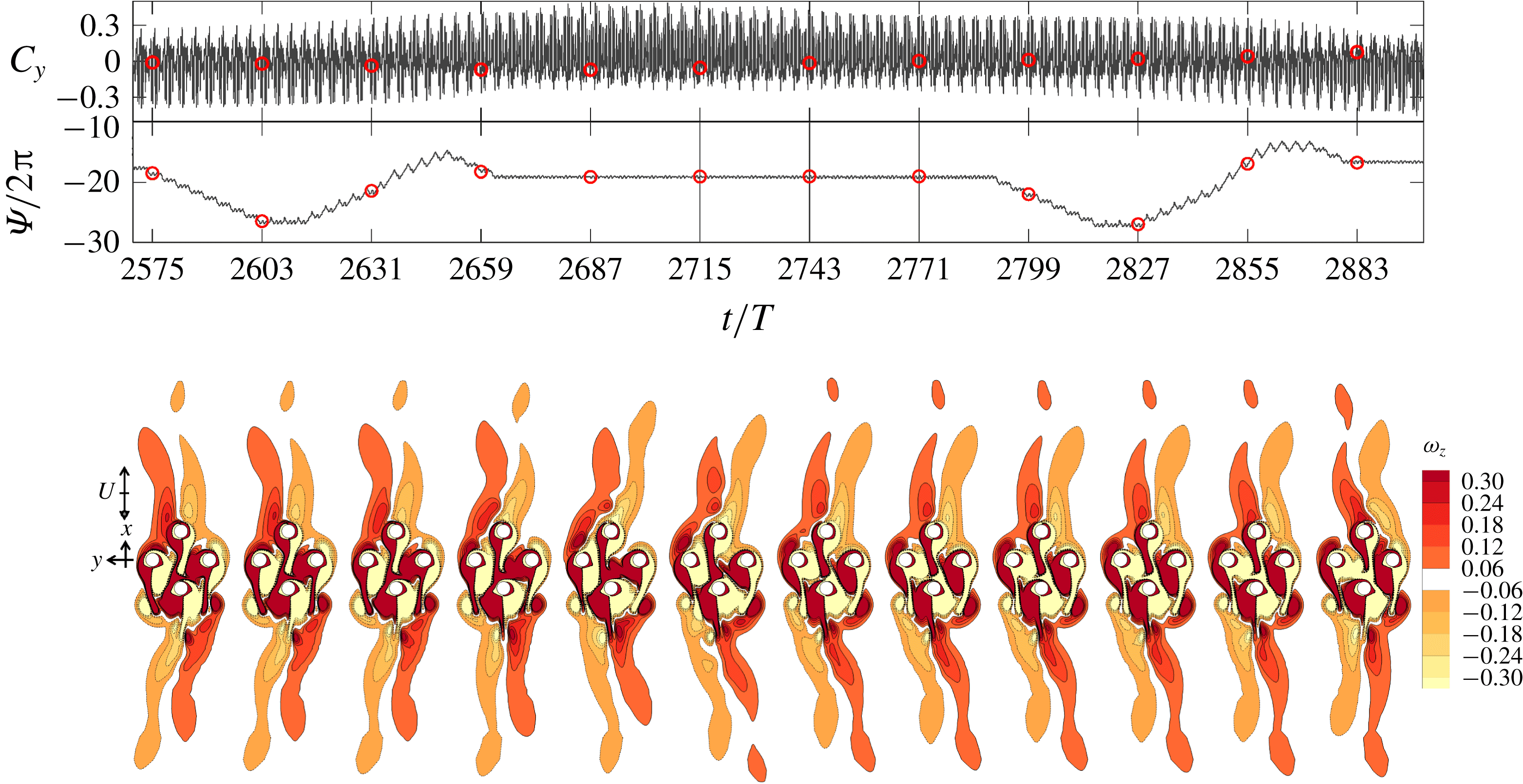
Figure 15 illustrates a typical regime
 $\text{D}_{1}^{\prime }$
flow at
 $(G,KC,Re)=(2,11,80)$
. The evolution of the streaklines for the regime
 $\text{D}_{1}^{\prime }$
flow in 20T is available in online supplementary movie ‘Movie 4.mp4’. The temporal variation of
 $C_{y}$
(figure 15
a) shows that the flow is quasi-periodic with a very long secondary period of approximately 43T. Figure 15(d) gives a close-up view of
 $C_{y}(t)$
over 43T enclosed by the red dash box in figure 15(a). The amplitude of
 $C_{y}(t)$
varies very slowly during the first 37T and experiences rapid variations in the next 6T, suggesting the overall flow is largely stable with instabilities being generated and dissipated periodically. There are two low frequency components in this case, one with a period of
 $T_{s1}\approx 6.173T$
and the other with
 $T_{s2}\approx 43.478T$
.
The phase dynamics shown in figure 15(b) is different from those of the synchronization states illustrated in figure 3(b). Since the response frequency appears in figure 15(e) is
 $f_{y}T=f_{l}T=2$
;
 $\unicode[STIX]{x1D6F9}$
oscillates with time at a frequency that is very close to
 $fT=2$
. To reveal the physics behind the specific features of
 $\unicode[STIX]{x1D6F9}(t)$
,
 $\overline{\unicode[STIX]{x1D6F9}_{T_{a}}}$
with
 $T_{a}=T$
is illustrated in figure 15(c), where a mixed mode of phase trapping and drifting exists and no obvious phase slipping is observed. The long period average of
 $\overline{\dot{\unicode[STIX]{x1D6F9}}_{T_{a}}}=0$
with
 $T_{a}=T_{s2}$
confirms that the phase of
 $C_{y}(t)$
is trapped with the phase of external forcing (
 $f_{l}T=2$
in (2.9)) over
 $T_{s2}$
.
Although phase trapping is routinely observed in other dynamic systems, it is rarely reported in bluff-body flows. Pikovsky et al. (Reference Pikovsky, Rosenblum and Kurths2003) demonstrated the occurrence of phase trapping through an amplitude equation under the condition of a large amplitude of external forcing with an increase of frequency detuning. When phase trapping occurs, the response has both amplitude and phase modulations, but the mean frequency of the response remains the same as that of the external forcing (Balanovet al.
Reference Balanov, Janson, Postnov and Sosnovtseva2008). The phase difference
 $\unicode[STIX]{x1D6F9}(t)$
is no longer a constant but oscillates around a constant value. The flow behaviour over
 $T_{s2}$
in our case fits well with the descriptions by Pikovsky et al. (Reference Pikovsky, Rosenblum and Kurths2003), suggesting the overall flow is dynamically stable but subject to strong disturbances, possibly due to flow instabilities local to the cylinder cluster. It follows from the phase trapping state that the mean response frequency
 $\langle f_{y}\rangle _{T_{s2}}$
equals
 $f_{l}$
.
Different from the phase drifting features observed in the other quasi-periodic flows and those illustrated in figures 10, 13 and 14, the phase drifts at different rates and towards different directions (upward and downward) in this case. Since
 $\langle f_{y}\rangle _{T_{s2}}=f_{l}$
, the rate of phase drifting is only dependent on the time derivative of
 $\unicode[STIX]{x1D719}_{i}(t)$
, based on (2.8). The different rates of drifting confirm the existence of multiple frequency components (or flow instabilities) and the frequent changes of drifting directions suggest that different instabilities dominate the response at different stages of flow development. It is believed that the unique feature of the phase dynamics displayed in this case is due to the complex interactions of flow instabilities developed around individual cylinders and the cylinder cluster. The cause of no obvious phase slipping is because the flow response
 $C_{y}(t)$
is largely synchronized with the incoming flow over the time period
 $T_{s2}$
shown in figure 15(d).
The flow structures observed in this case are examined to confirm the physics revealed by the phase dynamics. Figure 15(g) details the snapshots of vorticity contours at instants marked by the black stars in figure 15(d). The vorticity contours shown in figure 15(g) suggest that the slow variation of
 $C_{y}(t)$
is due to the slow flipping of the shear layers of the cluster (e.g. in the range from 352T to 376T in figure 15
d) and the shedding of vortices from the far tips of the shear layers (e.g. shedding in shear layer II from 386T to 394T). The relatively rapid variation of
 $C_{y}(t)$
is due to the asymmetric local vortex shedding around C2 and C4 (e.g. from 378T to 382T). The interactions of vortices a and b with neighbouring shear layers I and II in figure 15(g) are responsible for the strong oscillations of
 $C_{y}(t)$
. It takes a long period of time for the local flow to adjust back to the near synchronization state after the shedding of vortex from shear layer II.
The modulation features observed in figure 15(f) are different from those of quasi-periodic flows discussed so far and will be interpreted based on the phase dynamics. The existence of multiple frequency contents in the power spectrum of
 $C_{y}(t)$
shown in figure 15(f) confirms the interpretation based on the phase dynamics offered above. They can be classified into two groups, namely the response and secondary frequencies. The response frequency
 $f_{y}T$
of
 $C_{y}(t)$
is exactly 2, rather than near 2 as in the other quasi-periodic flows. The secondary frequency of
 $f_{s1}T=0.162$
(or
 $T_{s1}\approx 6.173T$
) corresponds to the rapid variation range in figure 15(d,g) and modulates odd-number peaks of
 $f_{u}T$
(frequencies at
 $fT=1$
and 3 are absent due to the overall 2-D state of the flow), but frequencies at
 $fT=2$
and 4 are unaffected. A number of low frequency components with negligible amplitudes occur near
 $f_{s2}T=0.023$
(orange peaks in figure 15
f), which modulate all the integer multiples of
 $f_{u}T$
. The disappearance of phase modulations at
 $fT=2$
and 4 can be explained by the phase trapping behaviour of the system. By substituting (2.8) and (2.9) into (2.7), taking the time derivative of
 $\unicode[STIX]{x1D6F9}(t)$
and averaging the resulting equation over
 $T_{a}=T_{s2}$
, we get
 $$\begin{eqnarray}\displaystyle \overline{\dot{\unicode[STIX]{x1D6F9}}_{T_{a}}}=2\unicode[STIX]{x03C0}\langle f_{y}\rangle _{T_{a}}-2\unicode[STIX]{x03C0}f_{l}+\langle \dot{\unicode[STIX]{x1D719}}_{i}(t)\rangle _{T_{a}}. & & \displaystyle\end{eqnarray}$$
Since the system satisfies
 $\overline{\dot{\unicode[STIX]{x1D6F9}}_{T_{a}}}=0$
and
 $\langle f_{y}\rangle _{T_{a}}=f_{l}$
in phase trapping behaviour, we know
 $\langle \dot{\unicode[STIX]{x1D719}}_{i}(t)\rangle _{T_{a}}=0$
. This result suggests that the frequency contents in
 $\unicode[STIX]{x1D719}_{i}(t)$
are
 $2\unicode[STIX]{x03C0}$
-periodic over the corresponding period. Therefore, no major phase modulation appears at even-number peaks of
 $f_{u}T$
.
Regime
 $\text{D}_{2}^{\prime }$
is only observed at
 $G=2$
when the flow transits from regime D or
 $\text{D}_{3}^{\prime }$
to the desynchronized flow zones (N). The features of a typical regime
 $\text{D}_{2}^{\prime }$
flow at
 $(G,KC,Re)=(2,11,90)$
are shown in figure 5(
 $i_{2}$
) and figure 16. The evolution of the streaklines for the regime
 $\text{D}_{2}^{\prime }$
flow in
 $20T$
is available in online supplementary movie ‘Movie 5.mp4’. The quasi-periodic feature of the flow, with a secondary period of 7T, can be observed from the temporal variation of
 $C_{y}$
and the power spectrum of
 $C_{y}(t)$
in figure 16(a) and (c), respectively. The phase trapping is also observed as
 $\unicode[STIX]{x1D6F9}(t)$
oscillates around a constant value around
 $-0.3\unicode[STIX]{x03C0}$
in figure 16(d). The secondary frequency component of
 $f_{s}T=0.142$
(or
 $T_{s}=7.042T$
) is associated with the cluster scale shedding of vortices (marked as I and II in figure 16
e) either side of the cylinder cluster. Since the oblique direction of the shear layers is always towards the negative direction of y, the mean
 $C_{y}$
is positive. The Lissajous phase diagram is symmetric about
 $C_{x}=0$
and the dominant peaks in the FFT spectrum of
 $C_{y}$
are located at the even-number peaks of
 $f_{u}T$
, as shown in figure 16(c), suggesting the flow holds
 $H_{1}$
symmetry. The frequency modulation disappears at the even-number peaks of
 $f_{u}T$
, but appears at the odd-number peaks as observed in the regime
 $\text{D}_{1}^{\prime }$
flow for the same reason as explained above.
Same as figure 10 but in a typical regime
 $\text{D}_{2}^{\prime }$
flow at
 $(G,KC,Re)=(2,11,90)$
.

Force characteristics of a typical regime
 $\text{D}_{3}^{\prime }$
flow at
 $(G,KC,Re)=(2,10,100)$
. Time traces of (a) the total lift coefficient and (b)
 $\unicode[STIX]{x1D6F9}$
, with a close-up view in (c) and (d), respectively; (e) Lissajous phase diagram of
 $C_{y}$
with
 $C_{x}$
and (f) FFT spectra of
 $C_{y}$
.

Regime
 $\text{D}_{3}^{\prime }$
is observed at
 $G=1$
and
 $G=2$
when one quasi-periodic flow transits to another quasi-periodic flow or regime N flow. A typical regime
 $\text{D}_{3}^{\prime }$
flow at
 $(G,KC,Re)=(2,10,100)$
is shown in figure 17 and figure 5(
 $i_{3}$
) (see also the online supplementary movie ‘Movie 6.mp4’). The temporal variation of
 $C_{y}$
shown in figure 17(a) and a close-up view in figure 17(c) suggest the existence of two additional low frequency components to the response frequency of
 $f_{y}T=2$
, one with a frequency of
 $f_{s1}T=0.141$
(or
 $T_{s1}\approx 7.092T$
) and the other with a frequency of
 $f_{s2}T=0.0024$
(or
 $T_{s2}\approx 414.667T$
) (figure 17
f). The large amplitudes of the peaks near
 $fT=1$
and 3 imply a high strength of the instabilities associated with
 $f_{s1}T=0.141$
. A close examination of the flow features (not shown here) in this case shows that the first low frequency component (
 $f_{s1}T=0.141$
) is associated with vortex shedding at the far tips of the shear layers either side of the cylinder cluster, in a similar manner to that shown in figure 16(e). The second low frequency component (
 $f_{s2}T=0.0024$
) is mainly due to the switching of oblique directions of the shear layers (flipping of the V-shape upside down), which will be detailed below.
The phase dynamics displayed in figure 17(b), which is characterized by epochs of phase trapping, intermingled with periods of phase drifting, is different from that observed so far. Each epoch of phase trapping corresponds to either a global peak or trough in the lift variations (figure 17
a) and generally lasts normally over 100T, followed by a period of phase drifting (both downwards and upwards). Although the mean
 $\unicode[STIX]{x1D6F9}$
values for the phase trapping epochs are different, they are integer multiples of
 $2\unicode[STIX]{x03C0}$
. If we shift the mean
 $\unicode[STIX]{x1D6F9}$
values for the phase trapping epochs to zero, the phase dynamics shown figure 17(b) would have the characteristics of a normal phase trapping behaviour. The stroboscopic views of vorticity contours sampled every
 $4T_{s1}$
in figure 18 confirm that the rapid variations of
 $\unicode[STIX]{x1D6F9}/2\unicode[STIX]{x03C0}$
(downwards and upwards drifts) are induced by the flipping of oblique directions (the V-shape) of the shear layers in the wake of the cluster. Each period of the downwards and upwards drift corresponds to a mirror reflection of the V-shape shear layers. When the oblique angle of ‘V’ reaches to the maximum (either direction), the flow becomes relatively stable over a long period of time during which the phase of the total lift is trapped with the phase of external forcing with
 $f_{l}T=2$
in (2.9). A typical phase slipping behaviour is observed during the lock-on period of
 $\unicode[STIX]{x1D6F9}$
in figure 17(d) and each period of phase locking and slipping lasts approximately
 $0.5T_{s1}$
. The slight differences between epochs of phase slipping are believed to be due to other minor flow instabilities.
Detailed lift coefficients, phase difference and vorticity contours for the case as shown in figure 17. The instantaneous vorticity contours are sampled every 28T (
 ${\approx}4T_{s1}$
) at the instants marked by ○ in the time traces diagrams.

The Lissajous phase diagram is symmetric about
 $C_{x}=0$
, suggesting the flow holds
 $H_{1}$
symmetry. The peaks of the power spectrum are expected to be dominated by even-number peaks (table 2), as shown in figure 17(f). No frequency modulation is observed around
 $fT=2$
because the second low frequency component (
 $f_{s2}T=0.0024$
) is too small and
 $C_{y}(t)$
is largely synchronized with the incoming flow. The amplitude modulation observed in figure 17(c) is mainly due to the first low frequency component of
 $f_{s1}T=0.141$
.
3.4 Desynchronized flows
The group of desynchronized flows refers to the flows that are not synchronous or quasi-periodic. The boundary lines between the synchronous/quasi-periodic flows and the desynchronized flows (the grey dashed line in figure 4) are estimated by interpolating the simulated cases at discrete points in the KC-Re space. For instance, the force features and flow pattern obtained from DNS at
 $(G,KC,Re)=(0.5,7,200)$
indicate the flow is in regime A, while a chaotic flow and force features are observed at
 $(0.5,7,210)$
in figure 21(a). So, at
 $KC=7$
, the boundary between regime A and regime N is determined as
 $Re=205$
. The symmetry-breaking boundary lines are therefore plotted by using a Bezier curve to fit these determined points.
3.4.1 Regime T
Regime T flows are characterized by irregular behaviours of the temporal variation of
 $C_{y}$
and breaking of all symmetry states specified in (1.2)–(1.4), as demonstrated by figure 19 at
 $(G,KC,Re)=(2,10,80)$
. Aperiodic features of
 $C_{y}(t)$
are observed in figure 19(a), which are clearly different from those observed in the synchronous and quasi-periodic flows. However, the power spectrum of
 $C_{y}(t)$
does show some regularities to a certain degree, which are difficult to quantify, based on the present knowledge of the authors. Sharp peaks are found near the integer multiples of
 $f_{u}T$
. Regime T flow is not classified as a regime N flow mainly because of the unusual location at which it occurs in the KC–Re space (see the close-up view in figure 4
c). The evolution of the streaklines in this case, as shown in figure 5(k) (see also the online supplementary movie ‘Movie 7.mp4’), reveals strong interactions of the flow processes local to the cylinder since a large number of particles remain in the vicinity of the cylinder cluster.
Force (a,b) and flow (c,d) characteristics of a typical regime T flow at
 $(G,KC,Re)=(2,10,80)$
. (a) Time traces of the total lift coefficient; (b) FFT spectrum of
 $C_{y}$
; Instantaneous vorticity contours in 10 oscillation periods in (c) and within one oscillation period in (d).

Similar to regime
 $\text{A}^{\prime }$
, regime T flows appear in an area surrounded by quasi-periodic flows. To identify the additional flow instabilities responsible for the occurrence of regime T flows, vorticity contours from period to period and within a typical flow period are examined in figure 19(c,d), respectively. The sizes of the shear layers become smaller and the shedding of vortices (figure 19
c) moves much closer to the cylinder cluster, compared with what is observed in the quasi-periodic flows, such as the case shown in figure 18. The shedding of vortices from individual cylinders and through the gaps between the cylinders is also apparent as shown in figure 19(d). The complex interactions of the shed vortices with shear layers formed around individual cylinders and the cluster as a whole are believed to be the cause for the irregular variations of
 $C_{y}(t)$
observed in figure 19(a) and the multiple frequency components appearing in figure 19(b). All symmetry states listed in (1.2)–(1.4) are broken, due to the complex interactions of flows mentioned above.
Regime maps for different configurations of the cylinder cluster by (a) only enlarging the distance between the two side cylinders to
 $(S/D)_{24}=5$
and (b) only enlarging the distance between the two in-line cylinders for
 $(S/D)_{13}=5$
. All the cases are based on
 $G=2$
. Cases for different regimes are marked with different symbols and colours as defined in figure 4(a).

To quantify the influence of flows around individual cylinders, two groups of additional simulations are carried out for a typical case with
 $G=2$
: (i) moving C2 and C4 further away from each other with a centre-to-centre distance of
 $(S/D)_{24}=5$
while maintaining the distance between C1 and C3, and (ii) moving C1 and C3 further away from each other with
 $(S/D)_{13}=5$
while maintaining the distance between C2 and C4. Local regime maps covering the same area as the close-up view in figure 4(c) for those two scenarios are shown in figure 20. For scenario (i), the regime T flows largely disappear and are replaced by synchronous and quasi-periodic flows (figure 20
a). For scenario (ii), however, regime T flows are still present for scenario (ii) (figure 20
b). Therefore, it is likely that the increase of distance between C2 and C4 reduces the interaction between the inner side shear layers of C2 and C4 and those from C1 and C3, which leads to the weakening of additional flow instabilities that trigger the occurrence of regime T flows. Although regime T flows are still present on increasing the distance between C1 and C3, the area occupied by regime T flows in the KC–Re space shrinks significantly. This observation appears to support the above inference that the complex interactions of shed vortices from individual cylinders (and also the cylinder cluster) and the shear layers formed around the cylinders and cylinder cluster are mainly responsible for the formation of regime T flows. The physical evidence of the appearance of regime T flow in a region surrounded by quasi-periodic regimes will be interpreted separately in § 4.1.2.
Flow characteristics of regime N near the symmetry-breaking boundary. Evolved from (a) regime A at
 $(G,KC,Re)=(0.5,7,210)$
; (b) regime
 $\text{C}^{\prime }$
at (0.5, 8, 200) and (c) regime D at (1, 12, 120).

3.4.2 Regime N
Most of the cases in each of the top-right corners of the regime maps (at large KC and Re) are named regime N, where complex flow patterns as well as strong interactions between flows around individual cylinders and the cluster as a whole are observed. A few examples of regime N flows are illustrated in figure 21 while the streaklines are shown in figure 5(
 $l_{1}$
–
 $l_{3}$
). Figure 21(a) shows a regime N flow that was evolved from regime A at
 $(G,KC,Re)=(0.5,7,210)$
, figure 21(b) shows a flow originated from regime C and figure 21(c) shows a flow directly transited from regime D. Two common features of regime N flows are (i) the symmetry breaking and (ii) the lack of regularity. Similar to the scenario of four-cylinder array in a square arrangement (Tong et al.
Reference Tong, Cheng, Zhao and An2015), the symmetry breaking can also evolve directly from
 $K_{y}$
symmetry at low KC number. It is believed that the complex interactions of multiple flow instabilities are responsible for the formation of regime N flows.
3.5 Summary of the regime maps
Overall, the flow regimes appear to be significantly influenced by G. At small gap ratios (
 $G=0.5$
and 1), the KC–Re space is dominated by synchronous flows since the oscillatory flow around the cluster at small gap ratios behaves in a similar way to oscillatory flow around a solid cylinder with a larger characteristic length scale, i.e. the cluster length scale W. The symmetry-breaking boundary occupies a smaller area at the top right corner of the regime map in comparison with that for the single cylinder because the increase of W leads to a smaller cluster-scale
 $KC_{w}$
which shifts the boundary to the top right of the KC–Re space. At the largest
 $G=4$
investigated in the present study, the KC–Re space is mainly occupied by flows with combined flow regimes (e.g.
 $4\text{A}/4\text{A}^{\ast }$
), and this observation is mainly because the cluster-scale effect is rather weak and the local-scale flow features around individual cylinders dominate the global flow response at this gap ratio. The interaction of flows around individual cylinders and around the cylinder cluster is strong with increasing G and is believed to be the main reason for most of the quasi-periodic flow regimes found at
 $G\geqslant 1$
. This interaction tends to destabilize the overall flow, as evidenced in the regime maps where regime N boundary moves towards the bottom left corner of the KC–Re space with increasing G.
4 Discussion
4.1 ‘Holes’ in the regime map
In addition to the rich flow regimes, figure 4 shows that: (i) at
 $G=1$
, quasi-periodic regime
 $\text{A}^{\prime }$
occurs in a region surrounded by synchronous regimes A and F; (ii) at
 $G=2$
, quasi-periodic regime
 $D_{1}^{\prime }$
occurs between synchronous regimes A and D at
 $KC=11$
(see the inset of figure 4
c); (iii) at
 $G=2$
, regime T flows occur in a region surrounded by quasi-periodic flows; and (iv) at
 $G=0.5$
, regimes F (with only
 $H_{2}$
symmetry) and D (with only
 $H_{1}$
symmetry) occur in an area occupied by regime A (with
 $K_{y}$
,
 $H_{1}$
and
 $H_{2}$
symmetry). The occurrence of those regimes in regions where they are not expected is rather strange and creates a few holes in the regime maps. The physical mechanisms responsible for the holes are explored in the following sections.
4.1.1 Physical presence of the holes
The first action that was undertaken was to ascertain that the holes are not artefacts of the numerical set-up. Apart from a careful mesh dependence check, as reported in appendix A, the influence of the time step on the results is further examined with
 $\unicode[STIX]{x0394}t=0.0005$
, 0.001 and 0.002 in the ranges of parameter space where the holes are found at
 $G=0.5$
. As detailed in § A.3, further reduction of time-step size does not affect the occurrence of the holes and has little influence on the hydrodynamic forces and global flow features.
The second action that was undertaken was to examine the sensitivity of the computational results to the initial conditions. To this end, further DNS simulations were performed at
 $(G,KC,Re)=(0.5,7,160)$
and (0.5, 8, 150) with a fully developed regime A flow from the adjacent upper and lower Re values as initial conditions (IC) of the simulation. For instance, the simulations for the case at
 $(G,KC,Re)=(0.5,7,160)$
was started from a fully developed instantaneous flow field of a lower Re at 150. As expected, different initial conditions did not affect the appearance of the holes. Hysteresis phenomenon is observed in the results presented in table 3, suggesting that the instability associated with scenario (iv) is subcritical in nature. For instance, at
 $(G,KC,Re)=(0.5,7,160)$
, regime F occurs with IC-0 and IC-Re150, but regime D occurs when initialized from IC-Re170.
Flow regimes based on simulations initialized from zero initial condition (IC-0) and non-zero IC.

The third action was to conduct linear (Floquet) stability analysis along four horizontal lines that cut through those regions in the regime maps (see the yellow areas in figure 4
a,b). No stability analysis was conducted for scenarios (ii) and (iii) because the base flows in scenario (ii) and (iii) become quasi-periodic or chaotic, and are not suitable for stability analysis. Given the holes consistently occur at
 $G=0.5$
, 1.0 and 2.0, they are likely induced by a similar physical mechanism. Therefore, the stability analysis conducted for scenarios (i) and (iv) would provide clues on the physics of the holes related to scenarios (ii) and (iii).
The stability analysis results are discussed in the following paragraphs. The convergence tolerance for the Floquet multiplier is set as
 $10^{-6}$
. The variation of
 $|\unicode[STIX]{x1D707}|$
and
 $\unicode[STIX]{x1D703}$
with Re are shown in figure 22. The critical bifurcation points are estimated by using a fourth-order extrapolation of
 $|\unicode[STIX]{x1D707}|$
to unity. The onset of
 $\unicode[STIX]{x1D703}$
at bifurcation points are predicted by using a fourth-order polynomial extrapolation of
 $\unicode[STIX]{x1D703}$
to the critical bifurcation points. Bifurcation points are plotted as vertical dashed lines in figure 22 in order to compare with the boundaries of the holes (shaded areas in figure 22) obtained from DNS. The convergence of the solution in the stability analysis is extremely slow for certain cases with marginal stability. For example, for the case at
 $(G,KC,Re)=(1,7,118)$
,
 $|\unicode[STIX]{x1D707}|=1.0014$
and
 $\unicode[STIX]{x1D703}=0.0075$
are obtained after 2000 iterations and these values fluctuate around the critical values of
 $|\unicode[STIX]{x1D707}|=1.0$
and
 $\unicode[STIX]{x1D703}=0.0$
. Such cases with slow convergence rates are marked as solid squares in figure 22. No further attempts are made to extend the number of iterations and those cases are considered as stable.
Variations of
 $|\unicode[STIX]{x1D707}|$
and
 $\unicode[STIX]{x1D703}$
of the Floquet multipliers with Re at (a)
 $(G,KC,Re)=(1,7,116{-}154)$
, (b) (1, 6, 156–210) and (c) (0.5, 7, 150–165). The open circles represent spurious multipliers. The solid squares represent the cases of marginal stable multipliers that are not converged until 2000 iterations. The red stars represent the angle (
 $\unicode[STIX]{x1D703}\approx 2\unicode[STIX]{x03C0}/T_{s}$
) computed from DNS data. The shaded areas represent the regions of holes obtained from DNS analysis.

For the case in scenario (i), where regime
 $\text{A}^{\prime }$
occurs in an area occupied by regimes A and F, the analyses are carried out at
 $G=1$
for
 $KC=7$
over the range of
 $Re=118$
to 154 and for
 $KC=6$
over the range of
 $Re=156$
to 210. The results for
 $KC=7$
are shown in figure 22(a), where
 $|\unicode[STIX]{x1D707}|$
is larger than 1 and
 $\unicode[STIX]{x1D707}$
becomes a complex-conjugate pair within the range of
 $Re=126$
–144 (
 $\unicode[STIX]{x1D703}\neq 0$
and
 $|\unicode[STIX]{x1D707}|>1$
). This result suggests the flow breaks
 $K_{y}$
symmetry and becomes quasi-periodic with a well-defined secondary frequency. The critical Re for the two bifurcation points at either end of regime
 $\text{A}^{\prime }$
are defined as
 $Re_{c1}$
and
 $Re_{c2}$
, respectively. The predicted values of
 $Re_{c1}=125.4$
and
 $\unicode[STIX]{x1D703}\approx 0.88$
and
 $Re_{c2}=146.1$
and
 $\unicode[STIX]{x1D703}\approx 1.06$
largely agree with the DNS results.
It is noted in some of the cases that the predicted magnitude of the Floquet multiplier is less than 1 with a non-zero
 $\unicode[STIX]{x1D703}$
, for example in the cases with
 $Re=122$
–124 and 146–148. The analysis does converge rapidly in those cases (shown in open circles in figure 22
a). A similar phenomenon was reported by Elston et al. (Reference Elston, Blackburn and Sheridan2006) and was referred to as a spurious multiplier. The occurrence of such cases was judged to be inherent to 2-D stability analyses and similar cases with spurious multipliers were subsequently considered as stable in Elston et al. (Reference Elston, Blackburn and Sheridan2006). The same practice as Elston et al. (Reference Elston, Blackburn and Sheridan2006) with regard to spurious multipliers is adopted in the present study.
The predicted
 $Re_{c1}=168.5$
and
 $\unicode[STIX]{x1D703}\approx 1.16$
for the onset of regime
 $\text{A}^{\prime }$
at
 $KC=6$
is consistent with the DNS results of
 $Re_{c1}=169.0$
and
 $\unicode[STIX]{x1D703}\approx 1.16$
. However, the stability analysis is unable to predict
 $Re_{c2}$
, probably due to the influence of nonlinear effects as Re moves further away from the bifurcation point, similar to the cases as discussed by Elston et al. (Reference Elston, Blackburn and Sheridan2006). The nonlinear effect can be inferred from the comparison of the secondary periods computed from DNS and stability analysis. The red stars in figure 22(a) represent the results from nonlinear solutions (DNS), where
 $\unicode[STIX]{x1D703}\approx 2\unicode[STIX]{x03C0}/T_{s}$
. The predicted
 $\unicode[STIX]{x1D703}$
values by DNS and stability analysis agree well with each other near
 $Re_{c1}$
where the nonlinear effect is small, whereas they depart from each other substantially as Re moves further away from
 $Re_{c1}$
with increasing nonlinear effects.
The phenomenon observed in the scenario (iv), where regimes F and D occur in an area occupied by regime A, has never been reported in oscillatory flow around a cylinder or cylinder clusters, to the best knowledge of the authors. The stability analysis is carried out at
 $G=0.5$
for
 $KC=7$
over a range of
 $Re=150$
to 165. It is observed in figure 22(c) that
 $\unicode[STIX]{x1D707}$
is real and crosses the unit circle at
 $Re=150.6$
–162.3, suggesting that although the
 $K_{y}$
symmetry is broken, no secondary frequency is involved and the flow is saturated into another synchronous state. This result is largely consistent with the DNS results shown in figure 4(a) where regimes F and D are observed at
 $Re=151$
–162.
The outcomes of § 4.1.1 appear to suggest that the holes are physical, rather than artefacts of the numerical set-ups. The ‘holes’ observed in regime maps of the present study is similar to the behaviours reported in steady flow past an oscillating cylinder (Ongoren & Rockwell Reference Ongoren and Rockwell1988; Papaioannou et al. Reference Papaioannou, Yue, Triantafyllou and Karniadakis2006; Perdikaris, Kaiktsis & Triantafyllou Reference Perdikaris, Kaiktsis and Triantafyllou2009). The physical mechanisms responsible for the holes were interpreted as the interaction of multiple flow instabilities and mode competition between the natural and forced modes. The quantitative and qualitative evidence of those holes in the present regime maps will be interpreted in § 4.1.2 as ‘mode competition’ between cylinder-scale and cluster-scale flows (due to flow through the gap).
4.1.2 Physical mechanism of the holes
Detailed evolutions of the flow for four representative cases for scenario (iv) are shown in figure 23. The vorticity contours with eight selected instants are plotted in a typical oscillatory period starting from
 $t_{0}$
when the flow is fully developed. A strong interaction of vortices around cylinders with those around the cylinder cluster is observed. For instance, at
 $(G,KC,Re)=(0.5,7,151)$
in figure 23(b) where the flow just transits from regime A to regime F, the vortex a around C2 appears to be stronger than its counterpart b around C4 and the interaction of vortex a with cluster-scale vortex I is clearly different from that between vortex b and cluster-scale vortex II, leading to the breaking of
 $K_{y}$
symmetry as shown in figure 23(b). A similar process occurs as the flow reverses. The clear mode competition between cylinder-scale and cluster-scale shear layers leads to the occurrence of regime F flow at
 $(G,KC,Re)=(0.5,7,155)$
. As Re is increased to
 $(G,KC,Re)=(0.5,7,160)$
, a stronger mode competition mechanism than that in the case of
 $(G,KC,Re)=(0.5,7,155)$
is observed in figure 23(c). A similar mode competition mechanism can also be observed in regime D flow (figure 23
d) at
 $(G,KC,Re)=(0.5,7,161)$
. After the transition back to regime A flow at
 $(G,KC,Re)=(0.5,7,163)$
, the interaction between flow around cylinder and cluster is noticeably weaker than the regime flows in the hole and the cluster-scale flow feature appears to dominate the flow response. A similar physical mechanism to those discussed above can also be observed in the flow features enclosed by blue dashed rectangles in figure 14(e), figure 15(g) and figure 19(d) for scenarios (i)–(iii) and will not be discussed further in detail.
Evolution of vorticity contours in one period at (a)
 $(G,KC,Re)=(0.5,7,150)$
in regime A; (b) (0.5, 7, 151) in regime F; (c) (0.5, 7, 160) in regime F; (d) (0.5, 7, 161) in regime D and (e) (0.5, 7, 163) in regime A.

Variations of averaged flow rates
 $\overline{Q_{in}}$
with Re from (1) the base flow, (2) the DNS and (3) mean drag coefficient computed from DNS at (a)
 $(G,KC)=(0.5,7)$
, (b)
 $(G,KC)=(1,7)$
. The shaded areas represent the regions of holes obtained from DNS analysis.

The increased level of interaction between cylinder-scale and cluster-scale flows in the parameter space covered by the holes is believed to be caused by the increased flow rate through the gaps facing the flow over the particular range of Re. To support this inference, the total flow rate
 $Q_{in}$
in half of a flow oscillation period is quantified as the following:
 $$\begin{eqnarray}Q_{in}=\int _{0}^{0.5T}\int _{s_{1}}v_{in}(t)\,\text{d}s_{1}\,\text{d}t+\int _{0}^{0.5T}\int _{s2}v_{in}(t)\,\text{d}s_{2}\,\text{d}t,\end{eqnarray}$$
where
 $v_{in}$
is the velocity perpendicular to
 $s_{1}$
or
 $s_{2}$
in figure 24(a). Equation (4.1) is applied to both the base flow used in the stability analysis and the flow obtained directly from DNS. The base flow is employed to ascertain that the changes of flow rate are not induced by flows in different regimes. Figure 24(a,b) shows the estimated average gap flow rate
 $\overline{Q_{in}}$
(over ten flow oscillation periods) at a number of points along two horizontal lines that cut through those regions in the regime maps at
 $(G,KC)=(0.5,7)$
and (1, 7). The clear increasing trends of
 $\overline{Q_{in}}$
with increasing Re over the parameter range covered by the holes are observed in both the base and DNS flows and along both lines. The rapid drops of
 $\overline{Q_{in}}$
(to comparable values of
 $\overline{Q_{in}}$
with that prior to the occurrence of the holes) are observed near the right boundaries of the holes. The above observation appears to confirm that the increased level of interaction between cylinder-scale and cluster-scale flows in the parameter space covered is caused by the increased flow rate through the gaps. The drop of
 $\overline{Q_{in}}$
near the right boundaries of the holes is the major reason that the flows recover to regime A in figure 24(
 $a_{1},a_{2}$
) and regime F in figure 24(
 $b_{1},b_{2}$
). The increase of
 $\overline{Q_{in}}$
in those cases covered by the holes is associated with a decreasing structure resistance to the flow, as quantified by the mean drag on the in-line cylinder pair C1 and C3 (
 $\overline{C_{D13}}$
) in figure 24(
 $a_{3},b_{3}$
). The
 $\overline{C_{D13}}$
is defined as the mean drag coefficient for in-line cylinders and is computed over 200 oscillatory periods based on the Morison equation (Morison, Johnson & Schaaf Reference Morison, Johnson and Schaaf1950). An opposite variation trend of
 $\overline{C_{D13}}$
to that of
 $\overline{Q_{in}}$
is observed for both cases, confirming the physical mechanism for the increase of
 $\overline{Q_{in}}$
over the particular range of the holes.
Variations of averaged flow rates
 $\overline{Q_{in}}$
with Re computed from DNS at (a)
 $(G,KC)=(2,10)$
, (b)
 $(G,KC)=(2,11)$
. The shaded areas represent the regions of different regimes obtained from DNS analysis.

The variations of
 $\overline{Q_{in}}$
with Re obtained from DNS are also quantified for the scenarios (ii) and (iii) along two horizontal lines cutting through the holes at
 $(G,KC)=(2,11)$
and (2, 10) respectively in figure 25. For scenario (iii) shown in figure 25(a),
 $\overline{Q_{in}}$
is almost a constant in regimes A and
 $\text{F}^{\prime }$
and experiences a rapid increase as the flow transits into regime T. This variation trend is similar to those observed in scenarios (i) and (iv). It is interesting to observe that
 $\overline{Q_{in}}$
continues its increasing trend and maintains almost a constant increase rate as Re crosses the upper bound boundary of regime T, which is different from the trends observed in scenarios (i) and (iv). The variation trend beyond regime T is considered reasonable because the flow in this parameter range is quasi-periodic. Since the slight increase of
 $\overline{Q_{in}}$
in regime T flows strengthens the cylinder-scale flows in the cluster and the cluster-scale flow is not weakened sufficiently due to the reduction of flow rate around the cluster, the interactions of the shear layers around individual cylinders and those around the cluster lead to the formation of regime T flows. With the further increase of Re, the shear layers around the cluster are weakened due to the reduced flow rate around the cluster and the cluster-scale flow becomes more stable, which leads to the observation of
 $\text{F}^{\prime }$
flow from
 $(KC,Re)=(10,90{-}95)$
. The flow transition into regime
 $\text{D}^{\prime }$
flows with the further increase of
 $Re>95$
can also be attributed to the large values of
 $\overline{Q_{in}}$
in regime
 $\text{D}^{\prime }$
flows. At this moment, the cluster-scale shear layers have been weakened significantly so that the cluster-scale flow becomes largely synchronized with local flows. Due to the strengthening of local flows by the large
 $\overline{Q_{in}}$
values, the cluster-scale flows in regime
 $\text{D}^{\prime }$
are considerably modulated by the local flow features as discussed in § 3.3.4. The above observation appears to confirm that the occurrence of the hole in scenario (iii) is due to the same flow mode competition mechanism as in scenarios (i) and (iv) outlined above.
The variation trend of
 $\overline{Q_{in}}$
with Re for scenario (ii) in figure 25(b) is very similar to that of scenario (iii) shown in figure 25(a). The same reasoning as that for scenario (iii) can be made and is not repeated. Again, the flow mechanism responsible for the occurrence of the hole in scenario (ii) is the flow mode competition, similar to the mechanism identified in other three scenarios.
4.2 Salient flow features of the diamond arrangement
Although oscillatory flow around four cylinders in a diamond arrangement shares some features observed in the corresponding flow around an isolated circular/square cylinder and four cylinders in a square arrangement (e.g. Tatsuno & Bearman Reference Tatsuno and Bearman1990; Elston et al. Reference Elston, Blackburn and Sheridan2006; Tong et al. Reference Tong, Cheng, Zhao and An2015, Reference Tong, Cheng, Xiong, Draper, An and Lou2017), it differs from those flows in that (i) the presence of gap distinguishes it from solid cylinders and (ii) the diamond cylinder arrangement induces a large flow blockage effect in comparison with four cylinders in a square arrangement. The above characteristics lead to certain salient flow features of four cylinders in a diamond arrangement, which are detailed below:
(1) The cluster-scale flow regimes of A and A* dominate the flow maps at small gap ratios of
$G=0.5$
and 1, in contrast to the dominance of parallel tandem-cylinders regime 2(A-A) in the square arrangement Tong et al. (Reference Tong, Cheng, Zhao and An2015).(2) The areas occupied by regime D flows in the regime map are much smaller than its counterparts in the circular/square cylinder (Tatsuno & Bearman Reference Tatsuno and Bearman1990; Tong et al. Reference Tong, Cheng, Xiong, Draper, An and Lou2017), as well as the square arrangement of four cylinders reported by Tong et al. (Reference Tong, Cheng, Zhao and An2015). Regime D flow was only observed at
$G=0.5$
in Tong et al. (Reference Tong, Cheng, Zhao and An2015), but appears at intermediate gap ratios (e.g.
$G=1$
and 2) when
$KC>11$
in the diamond arrangement.(3) A large number of quasi-periodic regimes are observed at
$G=2$
and 4 compared with a smaller region of quasi-periodic regimes identified in the square arrangement (Tong et al.
Reference Tong, Cheng, Zhao and An2015).(4) Quasi-periodic regime
$\text{D}^{\prime }$
(phase trapping) and period-doubling
$\text{A}^{\prime }$
(phase slipping) flows are first identified, which are associated with strong interactions of vortices shed from individual cylinders and flow instabilities developed in the wake of cylinder cluster.(5) The holes in the regime maps are observed consistently at
$G=0.5$
, 1 and 2 in the present study, whereas no such holes are observed in the square arrangement (Tong et al.
Reference Tong, Cheng, Zhao and An2015).


4.3 Three-dimensionality
Since the cluster-scale flow is a predominant feature in the diamond arrangement, three-dimensional (3-D) instabilities likely develop at relatively large Re or KC numbers near the symmetry-breaking boundary. To confirm this expectation, 3-D DNS is conducted at
 $(G,KC,Re)=(1,7,180)$
, which is close to the symmetry breaking boundary. A quasi-3-D approach, identical to the method detailed in Xiong et al. (Reference Xiong, Cheng, Tong and An2018b
), is employed. A spanwise length of
 $L_{z}=4\unicode[STIX]{x03C0}$
, and spanwise resolution
 $N_{z}=32$
are selected based on a detailed convergence test reported by Xiong et al. (Reference Xiong, Cheng, Tong and An2018b
).
Instantaneous flow features from 3-D simulations at two time instants of
 $t_{1}=50$
and
 $t_{2}=130$
at
 $(G,KC,Re)=(1,7,180)$
. (1) Instantaneous iso-surface of
 $\unicode[STIX]{x1D714}_{z}=\pm 0.25$
from and (2–3) spanwise-averaged cross-sectional vorticity. The red colour in (1) represents positive vorticity while the yellow denotes negative.

The simulation results sampled at
 $t/T=50$
and 130, shown in figure 26, demonstrate that three-dimensionality does develop near the symmetry-breaking boundary, as expected. Despite the obvious spanwise waviness of the iso-surfaces of
 $\unicode[STIX]{x1D714}_{z}$
, the spanwise-averaged cross-sectional flow features are similar to their counterparts obtained from 2-D simulation and largely retain the
 $H_{2}$
symmetry. This observation is consistent with previous findings in the literature (Nehari, Armenio & Ballio Reference Nehari, Armenio and Ballio2004; Tong et al.
Reference Tong, Cheng, Zhao and An2015; Xiong et al.
Reference Xiong, Cheng, Tong and An2018a
). Although 3-D flow features develop in most of the regimes other than
 $\text{A}^{\ast }$
and A, Nehari et al. (Reference Nehari, Armenio and Ballio2004) demonstrated that two-dimensional simulations are able to capture the cross-sectional flow features, which works especially well in regimes C–F. Tong et al. (Reference Tong, Cheng, Zhao and An2015) also demonstrated a similar point for oscillatory flow around four cylinders in a square arrangement and concluded that ‘three-dimensionality of the flow does not appear to significantly influence the cross-sectional flow fields or the onset of the symmetry-breaking regime’. An exception is that the Honji instability in regime B, characterized by mushroom-shape flows in the spanwise direction, cannot be captured by 2-D simulations (Honji Reference Honji2006; An, Cheng & Zhao Reference An, Cheng and Zhao2011). The present simulation results suggest that the boundary for 3-D instability could actually be lower than the boundary for regime N in the regime maps. Since mapping of this boundary represents a daunting task computationally and the primary objective of this study is on 2-D flow features, no further attempts are made to quantify this boundary.
5 Conclusions
This paper presents a 2-D DNS of oscillatory flow past a four-cylinder cluster in a diamond arrangement with four gap ratios of
 $G=0.5$
, 1, 2 and 4. Fourteen flow regimes are mapped out in a parameter space of
 $KC=4$
–12 and
 $Re=40$
–230, by means of flow visualizations, temporal variations of the total lift coefficient
 $C_{y}$
, the Lissajous phase diagrams of
 $C_{y}$
with
 $C_{x}$
and power spectra of
 $C_{y}$
. A number of quasi-periodic flow features observed from the simulations are interpreted through classical phase dynamics of a forced self-sustained oscillator. The major findings from this study are summarized below:
(I) Three types of flows, namely synchronous, quasi-periodic and desynchronized flows, are found over the investigated KC–Re space. The formation of different flow regimes is influenced by the flows around the cluster as a single body and individual cylinders. The synchronous flows are mainly found at small KC and Re values and small gap ratios where the flow around cluster scale dominates (regimes
$\text{A}/\text{A}^{\ast }$
, D and F), and also at large gap ratios (e.g.
$G=4$
) where the flow around cylinder scale dominates the global flow regimes (regimes
$4\text{A}/4\text{A}^{\ast }$
). Most of the quasi-periodic flow regimes
$\text{A}^{\prime }$
,
$\text{C}^{\prime }$
,
$\text{D}^{\prime }$
and
$\text{F}^{\prime }$
are observed at
$G\geqslant 1$
near the boundary of regime N flows where both cylinder and cluster length scales are important. Apart from regime N flows, the KC–Re space is mainly occupied by synchronous regime flows A and 4A at
$G=2$
and 4. The boundary of regime N flows moves towards the bottom left corner of the parameter space with increasing G.(II) The areas occupied by the regime D flows in the regime map are much smaller than their counterparts in the circular/square cylinder, as well as the square arrangement of four cylinders. The cause of the above feature is that significant flow blockage effect leads to a large cluster-scale
$KC_{w}$
. Therefore, a substantial reduction of regime D flows in the regime maps is observed at
$G=0.5$
. The cluster-scale effect is weakened with increasing G, which effectively increases the cluster-scale
$KC_{w}$
and therefore, several regime D flows exist at large KC values at
$G=1$
and 2. At large gap where
$G=4$
, the cluster-scale effect is rather weak and the interactions of flows around individual cylinders are attributed to the absence of regime D flows.(III) Three common features observed in quasi-periodic flows are: (i) the appearance of low frequency components
$f_{s}T$
that modulate the total lift on the cylinder cluster; (ii) the loss of regularity of the Lissajous phase diagram; and (iii) vortex shedding from the cylinder cluster and individual cylinders loses the synchronization with the oscillatory flow, but retains the synchronization flow features over periods that are significantly larger than the period of flow oscillation.(IV) The use of phase dynamics in the present study provides a new quantitative way of interpreting the physics involved in quasi-periodic flows, in addition to conventional methods such as frequency analysis. The phase analysis is instrumental in interpreting the synchronization behaviours between temporal variation trends of total lift on the cylinder cluster and the external forcing. It is instrumental in identifying the nature of the phase trapping regime
$\text{D}^{\prime }$
flows where the cluster-scale flow features are largely synchronized with the forcing of incoming oscillatory flow but are modulated by localized flow features.(V) The appearance of the secondary flow process in regimes
$\text{A}^{\prime }$
(period doubling),
$\text{C}^{\prime }$
and
$\text{F}^{\prime }$
is associated with instabilities developed in the wake of cylinder cluster. The incremental change processes of the shear layers formed around the cylinder cluster and vortex shedding from the far tips of the shear layers, which are the key flow mechanisms responsible for the quasi-periodic flows, correlate well respectively with the phase drifting and sudden phase slips quantified from the phase analysis. The degree of phase slip in each secondary period can be explained based on the circle maps introduced in this study.(VI) The strong interaction of vortices shed from individual cylinders and flow instabilities in the wake of the cluster are mainly associated with the occurrence of new regime
$\text{D}^{\prime }$
(phase trapping) flows. The low secondary frequency components only modulate odd-number peaks of
$f_{u}T$
while retain even-number peaks in the power spectra of total lift. The asymmetric shedding of vortices around the cylinder cluster and the slow shear layer oscillations are responsible for the appearance of two secondary frequency components in regime
$D_{1}^{\prime }$
. The shedding of vortices in the wake of the cluster of V-shape shear layers is associated with the appearance of secondary frequency in regime
$D_{2}^{\prime }$
, whereas the multiple low frequency contents in regime
$D_{3}^{\prime }$
are mainly induced by vortex shedding in the wake of the cluster and flipping of the vortex shedding direction around the cylinder cluster.(VII) Interactions of the vortex shedding processes from each of the in-line cylinder pair with those from side cylinder pair are mainly responsible for the occurrence of regime T flows. It is confirmed that the flows around side cylinders play a significant role in the occurrence of regime T flows.
(VIII) The ‘strange’ behaviours observed in the KC–Re parameter space, where (i) quasi-periodic flows occur in regions surrounded by synchronous flows (
$G=1$
and 2), (ii) aperiodic regime T flows occur in a region surrounded by quasi-periodic flows (
$G=2$
) and (iii) spatio-temporal symmetry flows occur in an area occupied by reflection symmetry flows (
$G=0.5$
), are confirmed to be physical through a careful dependence check of the time step and initial conditions, and stability analysis. The mode competition between cluster-scale and cylinder-scale flows is identified as the key physical mechanism responsible for those unique flow features, with the support of evidences derived from quantitative analysis.


Acknowledgements
The authors would like to acknowledge support from the National Key R&D Program of China (Project ID: 2016YFE0200100). This work was supported by resources provided by the Pawsey Supercomputing Centre with funding from the Australian Government and the Government of Western Australia.
Supplementary movies
Supplementary movies are available at https://doi.org/10.1017/jfm.2019.609.
Appendix A. Mesh convergence
A.1 Numerical validation for the case of a single cylinder
Prior to the mesh convergence study for the case of a four-cylinder cluster, the case of a single cylinder is investigated. For a single cylinder, the mesh uses
 $N_{c}=24$
elements around the cylinder surface, a polynomial expansion order
 $N_{p}$
of 6, a radial thickness of the element next to the cylinder surface
 $\unicode[STIX]{x0394}/D=0.035$
and a computational domain size of
 $(50.5+50.5)D\times (50.5+50.5)D$
, with the centre of the cylinder located at
 $(x,y)=(0,0)$
. The total element number
 $N_{el}$
is 1060 and the element mesh close to the cylinder is shown in figure 27(a).
The computational meshes around (a) a single cylinder and (b) a four-cylinder array (Mesh 1 in table 5). Each element contains
 $N_{p}^{2}$
quadrature points, while in the close-up view in (a),
 $N_{p}=6$
.

The mesh convergence for a single cylinder is checked at
 $(KC,Re)=(5,100)$
, where comparisons with numerical results in the literature (Dütsch et al.
Reference Dütsch, Durst, Becker and Lienhart1998; Zhao & Cheng Reference Zhao and Cheng2014; Tong et al.
Reference Tong, Cheng, Zhao and An2015) could be made. The hydrodynamic forces examined include the drag and inertia coefficients (
 $C_{D}$
and
 $C_{M}$
, respectively), and the r.m.s. in-line and lift coefficients (
 $C_{x}^{\prime }$
and
 $C_{y}^{\prime }$
, respectively). The drag and inertia coefficients for the cylinder are calculated through the least-square method using the in-line force on the cylinder over 200 flow oscillation periods based on the Morison equation (Morison et al.
Reference Morison, Johnson and Schaaf1950)
 $$\begin{eqnarray}\displaystyle F_{x}=\frac{1}{2}\unicode[STIX]{x1D70C}DC_{D}|u_{\infty }(t)|u_{\infty }(t)+\unicode[STIX]{x1D70C}\frac{\unicode[STIX]{x03C0}D^{2}}{4}C_{M}\frac{\text{d}u_{\infty }(t)}{\text{d}t}. & & \displaystyle\end{eqnarray}$$
It is seen in table 4 that the force coefficients of the present study are very close to the published results. In addition, the velocity profiles sampled along four lines
 $(x/D=-0.6,0,0.6,1.2)$
at
 $(KC,Re)=(5,100)$
are almost identical to those in Dütsch et al. (Reference Dütsch, Durst, Becker and Lienhart1998) and Xiong et al. (Reference Xiong, Cheng, Tong and An2018a
). The results mentioned above demonstrate that the numerical scheme based on Nektar++ is valid and the mesh quality is adequate.
Comparisons of the force coefficients for a single cylinder in oscillatory flow at
 $(KC,Re)=(5,100)$
. Note: FEM and FVM represents the finite element method and finite volume method that are employed for 2-D numerical simulation, respectively.

However, the mesh convergence was not checked at the extreme condition of
 $(KC,Re)=(12,230)$
, because this case belongs to the regime F flow where the inclined angles of two vortex streets change randomly with time (Dütsch et al.
Reference Dütsch, Durst, Becker and Lienhart1998; Nehari et al.
Reference Nehari, Armenio and Ballio2004). Since the force coefficients at
 $(KC,Re)=(12,230)$
are significantly affected by the length of the statistic period, it is difficult to separate the effects due to the computational mesh and the length of the statistic period for statistical analysis.
A.2 Mesh convergence study for the case of a four-cylinder cluster
For the present scenario of the four-cylinder cluster in a diamond arrangement, the computational domain size from each outer side of the cylinder cluster to the outer boundary is 50D, which is slightly larger than that used in Tong et al. (Reference Tong, Cheng, Zhao and An2015) (
 $100D\times 100D$
for the whole domain size) for the four-cylinder cluster in a square arrangement. In this way, the computational domain size varies from
 $(51.56+51.56)D\times (51.56+51.56)D$
for
 $G=0.5$
to
 $(54.35+54.35)D\times (54.35+54.35)D$
for
 $G=4$
.
Influence of the mesh sizes on hydrodynamic forces for oscillatory flow past the four-cylinder cluster at
 $(G,KC,Re)=(1,12,230)$
. Here
 $N_{el}$
is the total number of elements of the domain;
 $N_{p}$
is the polynomial order;
 $\unicode[STIX]{x1D6FC}_{2}$
and
 $\unicode[STIX]{x1D6FC}_{3}$
are the expansion ratios in the refined and outer regions respectively. The values in the brackets behind force coefficients are the relative errors compared with Mesh 1.

The mesh convergence study for the four-cylinder cluster configuration is carried out with
 $G=1$
. The mesh distribution close to the cylinder cluster is shown in figure 27(b). The mesh resolution, the expansion ratio around each individual cylinder (i.e.
 $\unicode[STIX]{x1D6FC}_{1}$
in the blue boxes in figure 27
a,b) and the expansion ratio in the outer region (i.e.
 $\unicode[STIX]{x1D6FC}_{3}$
the white regions in figure 27
a,b) are identical to those used for a single cylinder. Specifically, the radial size of the element next to the cylinder surface is 0.035D, the number of elements around each cylinder surface is
 $N_{c}=24$
, the polynomial expansion order
 $N_{p}$
is 6 and the expansion ratios
 $\unicode[STIX]{x1D6FC}_{1}$
and
 $\unicode[STIX]{x1D6FC}_{3}$
are 1.25 and 1.5, respectively.
According to previous studies on flow past multiple cylinders (Lam et al.
Reference Lam, Li, Chan and So2003; Zhao & Cheng Reference Zhao and Cheng2014; Tong et al.
Reference Tong, Cheng, Zhao and An2015), at relatively small gap ratios, the flow around the cylinder cluster is similar to that around a single body with an enlarged effective diameter. Therefore, in addition to the conventional mesh refinement around each individual cylinder, relatively high mesh resolutions are also used around the whole cylinder cluster (the expansion ratio
 $\unicode[STIX]{x1D6FC}_{2}$
= 1.1 within the grey region, i.e. the refined region, in figure 27
b).
Based on the mesh described above (called the reference mesh, or Mesh 1 in table 5), three variations are examined, as detailed in table 5:
(1) For Mesh 2, the polynomial expansion order
$N_{p}$
increases from 6 to 8.(2) For Mesh 3, the refined region (the grey region) is removed.
(3) For Mesh 4, the outer region (the white region) is refined.

The mesh convergence is checked by comparing the total hydrodynamic forces calculated with Meshes 2–4 to those calculated with the reference mesh (Mesh 1). The drag and inertia coefficients for the cylinder cluster are calculated by using the total in-line force in (A 1).
Simulations are first conducted for a periodic flow at
 $(G,KC,Re)=(1,5,100)$
(with
 $K_{y}$
symmetry) using different meshes. The results (not shown here) suggest that the hydrodynamics forces are converged to a four-figure accuracy. In addition, the streamwise velocity
 $U_{a}$
sampled along four lines at
 $x/D=-0.6,0$
and
 $y/D=0,0.6$
for different meshes at
 $t=t_{0}+1/6T$
are also compared. The maximum difference of
 $U_{a}$
values obtained using the above meshes and the reference mesh is 0.71 % of the free-stream velocity (
 $u_{\infty }=U_{m}\sin (1/6\unicode[STIX]{x1D714}T)=0.866$
).
Simulations are also conducted at
 $(G,KC,Re)=(1,12,230)$
, which involve the largest KC and Re values examined in this study. As shown in table 5, the hydrodynamic forces calculated with different meshes are within 1 % of the corresponding values obtained using the reference mesh, suggesting that the reference mesh listed in table 5 is adequate for the numerical simulations of the present study.
A.3 Time-step convergence check for holes at
$G=0.5$

In order to verify those holes in regime maps are not artefacts of the numerical set-ups, a detailed time-step dependence study was carried out for four cylinders in the diamond arrangement at two cases in the region of holes at
 $G=0.5$
. Detailed comparisons of hydrodynamic forces and flow features represented by vorticity contours are shown in table 6 and figure 28. Hydrodynamic forces calculated with different time steps in table 6 are within 1 % of the corresponding values obtained using the reference time step (
 $\unicode[STIX]{x0394}t=0.001$
) and the vorticity plots at the same time instant for different time steps show minor changes, suggesting further reduction of time-step size would not affect the occurrence of the holes and would show only minor influence on the hydrodynamic forces and global flow features.
Comparison on the vorticity contours at
 $t/T=400$
for (a)
 $(G,KC,Re)=(0.5,7,155)$
and (b)
 $=(0.5,8,150)$
. From top to bottom, the time steps for each row are set to 0.001, 0.0005 and 0.002.

Influence of time step on hydrodynamic forces for the oscillatory flow past the four-cylinder cluster at
 $G=0.5$
. Here
 $\unicode[STIX]{x0394}t$
is the time step used in each case. The values in the brackets behind the force coefficients are the relative errors compared with the reference time step of
 $\unicode[STIX]{x0394}t=0.001$
.

Appendix B. Summary of the flow regimes
The quantitative methods in identifying the flow regimes include: (i) the phase dynamics between the total lift coefficient and the far-field flow velocity; (ii) the temporal and spatial features of the flow field; (iii) the Lissajous phase diagram of the total in-line and lift coefficients; (iv) the FFT spectra of total lift coefficient; and (v) the characteristic length scales. Quantitative definitions of different flow regimes are summarized in table 7.
Summary of 14 oscillatory flow regimes of four cylinders in a diamond arrangement.