




1 Introduction
In low wind speeds of between 3 and  $6~\text{m}~\text{s}^{-1}$, interaction between wind-driven gravity–capillary waves and the wind-driven shear current leads to the generation of small-scale (centimetre-scale) Langmuir circulation (LC) in the water side of an air–water interface (Melville, Shear & Veron Reference Melville, Shear and Veron1988; Veron & Melville Reference Veron and Melville2001). These eddies consist of parallel counter-rotating vortices roughly aligned in the direction of the wind and waves. Small-scale LC structures were first observed by Langmuir (Reference Langmuir1938), and subsequently by Scott et al. (Reference Scott, Meyer, Stewart and Walther1969) and Kenney (Reference Kenney1993), and first studied quantitatively in the laboratory experiments of Melville et al. (Reference Melville, Shear and Veron1988) and later Veron & Melville (Reference Veron and Melville2001). In the experiments of Veron & Melville (Reference Veron and Melville2001), initiation of laminar LC (Li & Garrett Reference Li and Garrett1993; McWilliams, Sullivan & Moeng Reference McWilliams, Sullivan and Moeng1997) was followed by a sudden transition to turbulence in which the growing cells were characterized by irregularity while nonlinearly interacting with each other. More recently, such a transition has also been observed in the direct numerical simulation (DNS) of Hafsi, Tejada-Martínez & Veron (Reference Hafsi, Tejada-Martínez and Veron2017) following the Veron & Melville (Reference Veron and Melville2001) experiment.
The presence of aqueous turbulence serves to enhance near-surface vertical mixing resulting in a thinning of the molecular scalar diffusion sublayer and thus a greater scalar concentration gradient across the sublayer. The latter gives rise to an increase in scalar transfer across the air–water interface via molecular diffusion.
Recently, various highly resolved numerical simulations have been performed investigating the role of turbulence underneath gravity–capillary waves in determining scalar transport (either dissolved gas or heat transport) (e.g. see Komori et al. Reference Komori, Kurose, Iwano, Ukai and Suzuki2010; Tsai et al. Reference Tsai, Chen, Lu and Garbe2013; Takagaki et al. Reference Takagaki, Kurose, Tsujimoto, Komori and Takahashi2015; Kurose et al. Reference Kurose, Takagaki, Kimura and Komori2016; Hafsi et al. Reference Hafsi, Tejada-Martínez and Veron2017). Takagaki et al. (Reference Takagaki, Kurose, Tsujimoto, Komori and Takahashi2015), in a DNS configuration similar to that of Komori et al. (Reference Komori, Kurose, Iwano, Ukai and Suzuki2010) and Hafsi et al. (Reference Hafsi, Tejada-Martínez and Veron2017), observed that the aqueous turbulence underneath wind-driven, growing gravity–capillary waves is composed of two principal scales consisting of small intermittent surface motions embedded within larger growing scales. The latter grow in depth and width over time with the growing wave field. These larger eddies were identified as wind- and wave-driven centimetre-scale LC while the smaller scales were identified as purely shear-driven bursting motions characteristic of classical boundary layer turbulence. Furthermore, this small-scale shear-driven turbulence (and not the larger LC scales) was seen as controlling the near-surface turbulent scalar transport and thus responsible for setting the molecular diffusive scalar flux at the air–water interface. However, the role of the waves and associated LC in determining molecular diffusive scalar flux should be further investigated/clarified in light of the laboratory experiments of Veron & Melville (Reference Veron and Melville2001) and the DNS results of Komori et al. (Reference Komori, Kurose, Iwano, Ukai and Suzuki2010) and Hafsi et al. (Reference Hafsi, Tejada-Martínez and Veron2017). In particular, the DNS of Hafsi et al. (Reference Hafsi, Tejada-Martínez and Veron2017) and the earlier DNS of Komori et al. (Reference Komori, Kurose, Iwano, Ukai and Suzuki2010) suggest that the waves play a significant role by triggering the turbulence that leads to elevated values of molecular diffusive scalar flux at the air–water interface relative to DNS in which the sheared interface is intentionally held flat. In the latter case, the flow does not transition to turbulence. Veron & Melville (Reference Veron and Melville2001) also show that waves are the trigger to the laminar–turbulent transition in their physical experiments.
Langmuir turbulence is known to be comprised of a hierarchy of Langmuir cells, with smaller and more irregular cells occurring between stronger, more organized larger cells (Leibovich Reference Leibovich1983). A connection should be made between this hierarchy of cells and the small-scale bursting motions at the water surface identified by Takagaki et al. (Reference Takagaki, Kurose, Tsujimoto, Komori and Takahashi2015).
In this paper, the DNS of Hafsi et al. (Reference Hafsi, Tejada-Martínez and Veron2017) which follows closely that of Komori et al. (Reference Komori, Kurose, Iwano, Ukai and Suzuki2010) is revisited, highlighting the small-scale and larger-scale turbulence and the impact of the wave forcing on molecular diffusive scalar flux at the interface. Subsequently, large-eddy simulation (LES) of the water side is presented with the water surface taken as a rigid lid sheared by a constant wind stress with inclusion of the Craik–Leibovich (C–L) vortex force in the momentum equation parameterizing the effect of the waves and thus the LC-generating mechanism. This approach reveals similar structures highlighted in the DNS with a freely deforming air–water interface. Wave parameters (wavelength and amplitude) in the Stokes drift velocity in the C–L vortex force are varied in order to understand the effect of the wave forcing on the turbulence and ultimately the molecular diffusive scalar flux at the water surface and the turbulent vertical flux of the scalar throughout the water column. Analysis highlights the relationship between the small bursting surface motions and the larger scales of the turbulence and their impact on turbulent scalar transport, leading to the conclusion that the entire range of scales is dictated by the combined effect of the wind and wave forcing and is thus categorized as Langmuir turbulence.
2 Numerical set-up
2.1 The DNS and LES equations
The DNS is that of an air flow driving a water flow beneath (figure 1) with governing equations for both air and water consisting of the incompressible continuity and Navier–Stokes equations for the velocity  $(u,v,w)$ and pressure. The components
 $u$,
 $v$ and
 $w$ denote the velocity in the streamwise (or downwind) (
 $x$), spanwise (or crosswind) (
 $y$) and vertical (
 $z$) directions, respectively. The interface between the air and water is tracked via a volume-of-fluid method. In addition to the continuity and momentum (Navier–Stokes) equations to predict air and water flow velocities and pressures, the concentration of dissolved scalar (e.g. gas),
 $C$, in air and in water is predicted via an advection–diffusion equation. In this study, as is routinely done, the Schmidt number or ratio of kinematic viscosity to scalar diffusivity (
 $\unicode[STIX]{x1D708}/\unicode[STIX]{x1D705}$) is set to 1 because this does not affect the fundamental turbulent mechanisms promoting scalar transfer and transport. The interested reader is directed to Hafsi et al. (Reference Hafsi, Tejada-Martínez and Veron2017) for the DNS equations, and details of the volume-of-fluid method tracking the interface and the finite-volume-based numerical discretization.
(a) Coupled air–water flow DNS domain and computational mesh and (b) DNS flow domain and boundary conditions. Here  $z=0$ corresponds to the location of the unperturbed air–water interface. (c) The LES flow domain and boundary conditions where
 $z=0$ corresponds to the bottom of the domain. Length
 $\unicode[STIX]{x1D6FF}$ is 1.25 cm.

In the case of LES, the domain consists of only the water side with the water surface taken as a rigid lid driven by a constant wind stress in the  $x$-direction (figure 1). The wind stress is equal to the mean shear stress exerted by the air flow on the water surface in the DNS. The LES incompressible continuity and momentum equations are, respectively, as follows:
 $$\begin{eqnarray}\displaystyle & \displaystyle \frac{\unicode[STIX]{x2202}u_{i}}{\unicode[STIX]{x2202}x_{i}}=0, & \displaystyle\end{eqnarray}$$
 $$\begin{eqnarray}\displaystyle & \displaystyle \frac{\unicode[STIX]{x2202}u_{i}}{\unicode[STIX]{x2202}t}+u_{j}\frac{\unicode[STIX]{x2202}u_{i}}{\unicode[STIX]{x2202}x_{j}}=-\frac{\unicode[STIX]{x2202}\unicode[STIX]{x1D6F1}}{\unicode[STIX]{x2202}x_{i}}+\unicode[STIX]{x1D708}\frac{\unicode[STIX]{x2202}^{2}u_{i}}{\unicode[STIX]{x2202}x_{j}^{2}}+\frac{\unicode[STIX]{x2202}\unicode[STIX]{x1D70F}_{ij}}{\unicode[STIX]{x2202}x_{j}}+\unicode[STIX]{x1D716}_{ijk}V_{j}^{s}\unicode[STIX]{x1D714}_{k}, & \displaystyle\end{eqnarray}$$
where  $\unicode[STIX]{x1D716}_{ijk}$ is the totally antisymmetric third-rank tensor,
 $u_{i}$ and
 $\unicode[STIX]{x1D714}_{i}$ are the
 $i$th components of the LES (resolved) velocity and vorticity, respectively, in the Cartesian coordinate system (
 $x_{1}$,
 $x_{2}$,
 $x_{3}$),
 $t$ is time and
 $\unicode[STIX]{x1D708}$ is kinematic viscosity. For ease of notation, the downwind, crosswind and vertical velocities are denoted as
 $u_{1}=u$,
 $u_{2}=v$ and
 $u_{3}=w$, respectively. Furthermore, coordinates
 $x_{1}$,
 $x_{2}$ and
 $x_{3}$ are taken as
 $x$ (downwind),
 $y$ (spanwise) and
 $z$ (vertical), respectively.
The C–L vortex force is the last term on the right-hand side of the momentum equation above, where  $V_{j}^{s}$ is the Stokes drift velocity. The C–L vortex force consists of the cross-product between the Stokes drift velocity induced by the unresolved air–water interface waves and the flow vorticity (Craik & Leibovich Reference Craik and Leibovich1976; McWilliams et al. Reference McWilliams, Sullivan and Moeng1997; Fujiwara, Yoshikawa & Matsumara Reference Fujiwara, Yoshikawa and Matsumara2018). The C–L vortex force arises from wave-phase-averaging the momentum equation with the vertical shear of the Stokes drift velocity in this force serving to tilt vertical vorticity into streamwise vorticity and thus creating LC. Note that recent wave-phase-resolved formulations also exhibit this tilting mechanism (e.g. see Texeira & Belcher Reference Texeira and Belcher2002; Guo & Shen Reference Guo and Shen2013). Wave-phase-averaging also introduces a modified pressure (divided by constant density),
 $\unicode[STIX]{x1D6F1}$, appearing in the momentum equation. Pressure
 $\unicode[STIX]{x1D6F1}$ is given in terms of the static pressure and the Stokes drift; when the Stokes drift is zero
 $\unicode[STIX]{x1D6F1}$ reverts to the original static pressure. The definition of
 $\unicode[STIX]{x1D6F1}$ can be obtained from McWilliams et al. (Reference McWilliams, Sullivan and Moeng1997).
The Stokes drift velocity profile used for the present LES is based on the deep water wave approximation (Phillips Reference Phillips1977) taken with non-zero component in the downwind ( $x$) direction and zero components in the crosswind (
 $y$) and vertical (
 $z$) directions. Specifically, the downwind Stokes drift velocity is set as
 $$\begin{eqnarray}\displaystyle V_{1}^{s}=u^{s}=\left(\frac{2\unicode[STIX]{x03C0}A}{\unicode[STIX]{x1D706}}\right)^{2}\sqrt{\frac{g\unicode[STIX]{x1D706}}{2\unicode[STIX]{x03C0}}}\;\text{exp}\left[-4\unicode[STIX]{x03C0}\frac{(H-z)}{\unicode[STIX]{x1D706}}\right], & & \displaystyle\end{eqnarray}$$
where  $\unicode[STIX]{x1D706}$ and
 $A$ are the wavelength and amplitude, respectively,
 $g$ is gravitational acceleration and
 $H$ is the vertical length of the domain with
 $z$ extending from
 $z=0$ at the base (or bottom) to
 $z=H$ at the top (i.e. the water surface).
The LES advection–diffusion equation for scalar concentration is
 $$\begin{eqnarray}\displaystyle \frac{\unicode[STIX]{x2202}C}{\unicode[STIX]{x2202}t}+(u_{j}+V_{j}^{s})\frac{\unicode[STIX]{x2202}C}{\unicode[STIX]{x2202}x_{j}}=\unicode[STIX]{x1D705}\frac{\unicode[STIX]{x2202}^{2}C}{\unicode[STIX]{x2202}x_{j}^{2}}+\frac{\unicode[STIX]{x2202}q_{j}}{\unicode[STIX]{x2202}x_{j}}, & & \displaystyle\end{eqnarray}$$
where  $C$ is the LES (filtered) scalar concentration and
 $\unicode[STIX]{x1D705}$ is the diffusivity of the scalar in water.
The term  $\unicode[STIX]{x1D70F}_{ij}$ appearing on the right-hand side of the momentum equation in (2.2) and the term
 $q_{j}$ appearing on the right-hand side of the scalar transport equation in (2.4) are the LES subgrid-scale (SGS) stress and SGS scalar flux, respectively. Both the SGS stress and SGS scalar flux are modelled based on the well-known dynamic Smagorinsky model. These SGS models implemented for the present study are described in detail by Tejada-Martínez & Grosch (Reference Tejada-Martínez and Grosch2007) and Akan et al. (Reference Akan, Tejada-Martínez, Grosch and Martinat2013).
The LES numerical discretization solving the continuity, momentum and scalar transport equations numerically consists of a fractional step scheme together with a hybrid spectral/(fifth- and sixth-order) finite-difference scheme for spatial derivatives. This discretization is presented by Tejada-Martínez & Grosch (Reference Tejada-Martínez and Grosch2007) and Tejada-Martínez et al. (Reference Tejada-Martínez, Grosch, Gargett, Polton, Smith and MacKinnon2009).
2.2 Computational domain: mesh and boundary and initial conditions
The DNS flow domain shown in figure 1 consists of a rectangular box with height  $3\unicode[STIX]{x1D6FF}$ and streamwise (downwind) and spanwise (crosswind) lengths of
 $8\unicode[STIX]{x1D6FF}$ and
 $4\unicode[STIX]{x1D6FF}$, respectively, where
 $\unicode[STIX]{x1D6FF}=1.25~\text{cm}$. The air side occupies the upper portion of the domain with height
 $\unicode[STIX]{x1D6FF}$ and the water side occupies the lower portion with depth
 $2\unicode[STIX]{x1D6FF}$. Streamwise and spanwise directions are given by the
 $x$-axis and the
 $y$-axis, respectively, while the
 $z$-axis spans the air and water depths. The unperturbed air–water interface is located at
 $z=0$.
The DNS mesh and boundary conditions are summarized in figure 1. The water side was started from rest with a flat air–water interface driven from above by the sudden imposition of a precomputed, fully developed boundary layer air flow driven by a pressure gradient in the  $x$-direction. This boundary layer air flow was precomputed (as a first step) in a separate simulation with a no-slip bottom and a zero-shear-stress condition on top while maintaining periodic boundary conditions elsewhere (along
 $x$- and
 $y$-directions). The precomputed air flow was characterized by free-stream mean velocity
 $U_{\infty }=5~\text{m}~\text{s}^{-1}$, which is the same as the final free-stream wind speed in one of the experiments of Veron & Melville (Reference Veron and Melville2001). For consistency, the computational domain and mesh to run the preliminary air flow simulation were identical to those of the air-side portion of the coupled air–water flow domain in figure 1.
The precomputed air flow with  $U_{\infty }=5~\text{m}~\text{s}^{-1}$ imposed as an initial condition results in a nominal air friction velocity (
 $u_{\unicode[STIX]{x1D70F}}^{a}$) of
 $0.25~\text{m}~\text{s}^{-1}$ and a nominal water friction velocity (
 $u_{\unicode[STIX]{x1D70F}}^{w}$) of
 $0.0087~\text{m}~\text{s}^{-1}$ in DNS of the air–water coupled boundary layers. Hence for the air side, the friction Reynolds number is
 $Re_{\unicode[STIX]{x1D70F}}^{a}=u_{\unicode[STIX]{x1D70F}}^{a}\unicode[STIX]{x1D6FF}/\unicode[STIX]{x1D708}_{a}=208$ based on the height of the air domain with the kinematic viscosity for air (
 $\unicode[STIX]{x1D708}_{a}$) taken as
 $1.5\times 10^{-5}~\text{m}^{2}~\text{s}^{-1}$. For the water side, the friction Reynolds number is
 $Re_{\unicode[STIX]{x1D70F}}^{w}=u_{\unicode[STIX]{x1D70F}}^{w}2\unicode[STIX]{x1D6FF}/\unicode[STIX]{x1D708}_{w}=217$ based on the height of the water domain with kinematic viscosity for water (
 $\unicode[STIX]{x1D708}_{w}$) taken as
 $10^{-6}~\text{m}^{2}~\text{s}^{-1}$.
The initial condition for scalar concentration was  $C=1~\text{mol}~\text{m}^{-3}$ in the air side and
 $C=0$ in the water side. At the top of the domain (at the top of the air side)
 $C$ was set to
 $1~\text{mol}~\text{m}^{-3}$ and at the bottom of the domain (the bottom of the water side)
 $C$ was set to 0, ensuring an air side saturated with scalar and thus a flux of scalar from the air side to the water side.
In the DNS, the air side of the computational mesh shown in figure 1(a) consists of 200 points in the  $x$-direction, 100 points in the
 $y$-direction and 60 points in the
 $z$-direction (200 by 100 by 60). Meanwhile the water side consists of 200 by 100 by 120 grid points. Mesh sizes along
 $x$ and
 $y$,
 $\unicode[STIX]{x0394}x$ and
 $\unicode[STIX]{x0394}y$, respectively, are uniform, with
 $\unicode[STIX]{x0394}x=\unicode[STIX]{x0394}y=0.05~\text{cm}$. Refinement is applied in
 $z$ such that vertical mesh size
 $\unicode[STIX]{x0394}z$ decreases in the approach to the air–water interface from either the water side or the air side. The refinement in the vertical allows resolution of the air–water interface including millimetre-scale interfacial deformations in the case of DNS as well as the molecular sublayers in the air and water sides. Vertical grid resolution is between approximately 0.006 cm (near the air–water interface) and 0.05 cm (near the top and bottom of the domain).
Normalizing the grid resolutions above by appropriate viscous length scales results in the following mesh sizes. For the air side,  $\unicode[STIX]{x0394}x^{+}=\unicode[STIX]{x0394}xu_{\unicode[STIX]{x1D70F}}^{a}/\unicode[STIX]{x1D708}_{a}$ and
 $\unicode[STIX]{x0394}y^{+}=\unicode[STIX]{x0394}yu_{\unicode[STIX]{x1D70F}}^{a}/\unicode[STIX]{x1D708}_{a}$ are both 16.6. Also for the air side,
 $\unicode[STIX]{x0394}z^{+}=\unicode[STIX]{x0394}zu_{\unicode[STIX]{x1D70F}}^{a}/\unicode[STIX]{x1D708}_{a}$ varies from 1 at the interface to 8.32 at the top of the air domain. Meanwhile for the water side,
 $\unicode[STIX]{x0394}x^{+}=\unicode[STIX]{x0394}xu_{\unicode[STIX]{x1D70F}}^{w}/\unicode[STIX]{x1D708}_{w}$ and
 $\unicode[STIX]{x0394}y^{+}=\unicode[STIX]{x0394}yu_{\unicode[STIX]{x1D70F}}^{w}/\unicode[STIX]{x1D708}_{w}$ are both 4.34. Furthermore, for the water side,
 $\unicode[STIX]{x0394}z^{+}=\unicode[STIX]{x0394}zu_{\unicode[STIX]{x1D70F}}^{a}/\unicode[STIX]{x1D708}_{a}$ varies from 0.52 at the interface to 4.33 at the bottom of the water domain.
The LES was performed without resolution of waves at the air–water interface; hence the domain (shown in figure 1c) was taken to be solely the water-side portion of the DNS domain in figure 1(b) with  $z$ extending from 0 at the bottom of the domain to
 $z=0.025~\text{m}$ at the top of the domain (i.e. the water surface). The water surface was taken as a rigid lid driven by a constant wind stress in the
 $x$-direction. The latter results in the same friction Reynolds number as noted earlier for the water side of the DNS, i.e.
 $Re_{\unicode[STIX]{x1D70F}}^{w}=217$. The scalar concentration was fixed at
 $C=1~\text{mol}~\text{m}^{-3}$ at the rigid lid, mimicking a scalar-saturated air side as in the DNS. The boundary conditions at the bottom of the LES domain were the same as those for the DNS domain (see figure 1). The scalar concentration was set to zero as the initial condition for the LES. The water flow was initialized from rest but for small random perturbations of the downwind velocity at the surface in order to facilitate transition to turbulence. The initial state was suddenly forced by the constant wind stress mentioned above in all of the LES cases and wave forcing through the C–L vortex force in the LES momentum equation in the flows with LC.
The near-rest initial condition shared by all LES cases consisted of zero scalar concentration, zero pressure and zero velocity everywhere, except at the surface where a perturbation of the downwind velocity was given as  $0.001\unicode[STIX]{x1D701}~\text{m}~\text{s}^{-1}$, with
 $\unicode[STIX]{x1D701}$ a pseudo randomly generated integer between 0 and 1. Note that this perturbation is an order of magnitude smaller than the surface downwind velocity fluctuations associated with LC obtained in the LES (to be shown later in figures 9a,b and12a,b).
The LES mesh was coarser than the DNS mesh of the water side. The LES mesh consisted of 33 and 65 points in  $x$ and
 $y$, respectively, resulting in
 $\unicode[STIX]{x0394}x^{+}=27.2$ and
 $\unicode[STIX]{x0394}y^{+}=6.78$. A variable mesh size was adopted in the vertical direction with
 $\unicode[STIX]{x0394}z_{1}^{+}=1$ being the surface-normal distance between the surface and the first grid point below the surface. The LES discretization and resolution employed have been shown by Tejada-Martínez et al. (Reference Tejada-Martínez, Grosch, Gargett, Polton, Smith and MacKinnon2009) to yield good agreement with DNS for turbulent channel flows at relatively low friction Reynolds number similar to that considered here (
 $Re_{\unicode[STIX]{x1D70F}}^{w}=217$).
3 Results
3.1 Direct numerical simulation
Soon after the DNS started, at time  $t=1.5~\text{s}$, short capillary interfacial waves as small as 1 cm in wavelength and 0.25 mm in height were present accompanied by small ripples with length scales of approximately 1 to 2 mm. These waves grew in amplitude and wavelength in time reaching the gravity–capillary regime, and after 6.5 s the simulation was stopped once the wave amplitude reached a size comparable to the height of the air-side domain. Details of the gravity–capillary waves obtained including the good agreement with the gravity–capillary waves simulated by Komori et al. (Reference Komori, Kurose, Iwano, Ukai and Suzuki2010) and Takagaki et al. (Reference Takagaki, Kurose, Tsujimoto, Komori and Takahashi2015) are provided by Hafsi et al. (Reference Hafsi, Tejada-Martínez and Veron2017) (for example, see figure 5 of Hafsi et al.). Here, presentation of results is limited in terms of the aqueous turbulent structures obtained and the associated scalar transfer across the air–water interface.
3.1.1 Turbulent scales
Soon after the appearance of capillary waves, the flow underneath transitioned to turbulence at  $t\sim 2~\text{s}$, and following Takagaki et al. (Reference Takagaki, Kurose, Tsujimoto, Komori and Takahashi2015), the turbulent structures resolved can be observed via instantaneous scalar concentration distribution over a cross-sectional spanwise–vertical (
 $y$–
 $z$) plane at a fixed
 $x$, as shown in figure 2. The turbulence is characterized by two principal structures: (1) centimetre-scale LC which at
 $t=6.5~\text{s}$ occupies most of the water side of the domain and (2) smaller bursting motions at the surface embedded within the centimetre-scale LC. Initially the centimetre-scale Langmuir cells are smaller than those shown in figure 2, and over time grow in depth and spanwise length. As seen in figure 2, by time
 $t=6.5~\text{s}$, the largest scale consists of two pairs of centimetre-scale LC spanning the width of the domain. In this figure, it can be seen that the downwelling limbs of the centimetre-scale LC bring high-concentration fluid from the surface to depths below, while the upwelling limbs bring low-concentration fluid close to the surface.
Turbulent structures at  $t=6.5~\text{s}$ in terms of scalar concentration (
 $\text{mol}~\text{m}^{-3}$) in DNS with a deformable air–water interface in the form of gravity–capillary waves. Downward arrows denote either the downwelling limb of a Langmuir cell or a smaller-scale eddy at the surface. The upward arrow corresponds to an upwelling limb of the LC.

The activity of the smaller-scale bursting motions at the surface embedded within the centimetre-scale LC can be observed in figure 2 through small filaments of high-concentration fluid ejected from the surface within the larger-scale vertical scalar transport pattern induced by the downwelling and upwelling limbs of the centimetre-scale LC. The ejections of high-concentration fluid from the surface are transported further down by the downwelling limbs of the large LC. As noted by Takagaki et al. (Reference Takagaki, Kurose, Tsujimoto, Komori and Takahashi2015), these ejections serve to peel the molecular diffusive boundary layer of the scalar, thereby helping to set the gradient of scalar across the boundary layer and thus the transfer of scalar across the air–water interface via molecular diffusion.
Takagaki et al. (Reference Takagaki, Kurose, Tsujimoto, Komori and Takahashi2015) showed that the small-scale bursting motions are characterized by high- and low-speed streaks in the downwind velocity fluctuations on the air–water interface coinciding with low and high scalar flux streaks, respectively, on the interface. The high- and low-speed streaks were shown to possess similar characteristics to the well-known high- and low-speed streaks in classical shear-dominated boundary layers (Smith & Metzler Reference Smith and Metzler1983). This suggests that the small-scale bursting motions were purely driven by the wind shear.
The distinct size of the centimetre-scale LC from the rest of the turbulence seen in figure 2 enabled Takagaki et al. (Reference Takagaki, Kurose, Tsujimoto, Komori and Takahashi2015) to perform a scale decomposition to determine the contribution of this LC scale to the turbulent vertical scalar flux compared to that of the smaller-scale turbulence. For their DNS they concluded that in general the near-surface turbulent vertical transport of the scalar is controlled by the small-scale turbulence, i.e. the wind-shear-driven small-scale bursting motions, and not by the wind- and wave-driven larger-scale LC. This implies that the small-scale wind-shear-driven turbulence also controls the scalar diffusive flux across the air–water interface.
3.1.2 Molecular diffusive scalar flux at the surface and transition to turbulence
Molecular diffusive flux of the scalar at the air–water interface is defined as  $F=\unicode[STIX]{x1D705}\unicode[STIX]{x1D735}C\boldsymbol{\cdot }\boldsymbol{n}$, where
 $\unicode[STIX]{x1D705}$ is the scalar molecular diffusivity, the gradient of concentration,
 $\unicode[STIX]{x1D735}C$, is evaluated at the air–water interface and
 $\boldsymbol{n}$ is the normal to the interface. Transition to turbulence in the water side of the DNS occurs at about
 $t=2~\text{s}$ and is accompanied by a spike of approximately an order of magnitude in
 $F$ averaged over the interface, i.e.
 $\langle F\rangle _{interface}$, shown in figure 3. As can be seen in this figure, the spike in
 $\langle F\rangle _{interface}$ is noticeably absent in a DNS run repeated but with the air–water interface intentionally held flat (i.e. DNS without waves/LC) suggesting strong dependence of the flux on wave forcing. As can also be seen in figure 3, after transition to turbulence occurs, the DNS with waves/LC exhibits a statistically steady value in the time series of
 $\langle F\rangle _{interface}$ about eight times greater than in the DNS with air–water interface held flat, suggesting the importance of the wave forcing and associated LC for the molecular diffusive flux across the air–water interface. A similar result was obtained by Komori et al. (Reference Komori, Kurose, Iwano, Ukai and Suzuki2010) in terms of transfer velocity (a measure of scalar transfer efficiency across the air–water interface) averaged over the air–water interface.
Time series of the molecular diffusive flux of the scalar ( $\text{mol}~\text{m}^{-2}~\text{s}^{-1}$) at the air–water interface in DNS with gravity–capillary waves (i.e. deforming interface case) and DNS with air–water interface intentionally held flat (i.e. flat interface case). The flux was averaged over the interface.

The previous comparison between DNS with and without waves suggests the importance of wave forcing in determining  $\langle F\rangle _{interface}$. However, this stands in contrast with the conclusion of Takagaki et al. (Reference Takagaki, Kurose, Tsujimoto, Komori and Takahashi2015) that
 $\langle F\rangle _{interface}$ is determined solely by the purely wind-shear-driven small bursting motions at the water surface and not by the wind- and wave-driven LC motions. The LES results are presented next, further exploring the effect of the wind and wave forcing on the turbulence and ultimately on
 $\langle F\rangle _{interface}$ and the turbulent vertical flux of the scalar throughout the water column.
3.2 Large-eddy simulation
The LES was performed with the domain configuration and mesh introduced earlier. In LES of small-scale LC, the momentum equation was augmented with the C–L vortex as given in (2.2) with the water surface taken as a wind-sheared rigid lid. Additionally, the advecting velocity in the transport equation for scalar concentration was augmented with the Stokes drift as seen in (2.4). The C–L vortex force represents the generating mechanism of the LC scales (i.e. the wave–current interaction) without the need to resolve the interfacial waves. The formulation allows direct input of the Stokes drift velocity in (2.3) facilitating study of the impact of wave forcing parameters on the turbulent structures and ultimately the scalar transfer across the air–water interface via molecular diffusion. Three LESs were performed characterized by different wavelengths ( $\unicode[STIX]{x1D706}$) and amplitudes (
 $A$) in (2.3): LES-A, LES-B and LES-C. In LES-A,
 $\unicode[STIX]{x1D706}=1~\text{cm}$ and
 $A=0.0707~\text{cm}$, values that are characteristic of the waves at the onset of the turbulence in the DNS of Komori et al. (Reference Komori, Kurose, Iwano, Ukai and Suzuki2010) and Hafsi et al. (Reference Hafsi, Tejada-Martínez and Veron2017). Obtaining the Stokes drift velocity at the water surface (denoted as
 $u_{o}^{s}$) from (2.3), the turbulent Langmuir number defined as
 $La_{t}=\sqrt{u_{\unicode[STIX]{x1D70F}}^{w}/u_{o}^{s}}$ (McWilliams et al. Reference McWilliams, Sullivan and Moeng1997) is calculated as
 $La_{t}=0.63$. Here
 $La_{t}$ is inversely proportional to the strength of wave forcing relative to wind forcing, and thus the turbulence in LES-A is expected to be Langmuir-dominated. The wave parameters in LES-B and LES-C represent idealized variations of the parameters in LES-A in order to highlight the impact of the wave forcing and thus LC on the turbulent scalar transport. Case LES-B is characterized by the same surface Stokes drift value (
 $u_{o}^{s}$) as LES-A (and thus has
 $La_{t}=0.63$), but with a longer wavelength
 $\unicode[STIX]{x1D706}=10~\text{cm}$. Simulation LES-C was performed with
 $\unicode[STIX]{x1D706}=10~\text{cm}$ and
 $La_{t}=0.4$. The Stokes drift and Stokes drift vertical shear are plotted in figure 4 for LES-A, LES-B and LES-C. The Stokes drift shear serves to promote the growth of LC (Holm Reference Holm1996), and LES-B and LES-C are expected to be characterized by more vigorous LC deeper into the water column given their greater Stokes drift shear at depths below the water surface compared to LES-A. Finally, a fourth simulation denoted as LES-D was performed without the C–L vortex force in (2.2) and without the advecting Stokes drift velocity in (2.4); thus this case was purely wind-driven. Table 1 presents a summary of the LES and DNS simulations performed.
(a) Stokes drift velocity  $u^{s}$ (
 $\text{m}~\text{s}^{-1}$) and (b) Stokes drift velocity shear
 $\text{d}u^{s}/\text{d}z$ (
 $\text{s}^{-1}$) in the LES simulations performed with C–L vortex forcing.

Summary of the wave conditions in the LES and DNS performed. Wave amplitude and wavelength in DNS with deforming interface are time-dependent. These wave parameters are constant in LES-A, LES-B and LES-C and are given through wavelength  $\unicode[STIX]{x1D706}$ and turbulent Langmuir number
 $La_{t}$.

3.2.1 Molecular diffusive scalar flux at the surface and transition to turbulence
Similar to the DNS, the flows in LES-A, LES-B and LES-C undergo transition to turbulence starting from near rest driven by the wind and wave forcing. This can be seen in figure 5 by the sudden spikes in the time series of turbulent kinetic energy (defined as  $[\langle u^{\prime 2}\rangle +\langle v^{\prime 2}\rangle +\langle w^{\prime 2}\rangle ]/2$) near the surface and the average molecular diffusive scalar flux (defined as
 $\unicode[STIX]{x1D705}\;\text{d}\langle C\rangle /\text{d}z$) at the surface. In these expressions, the angle brackets denote averaging over downwind (
 $x$) and crosswind (
 $y$) directions. The transition to turbulence in LES-B is delayed relative to LES-A and LES-C, which is attributed to the lower surface Stokes drift shear in this case (see figure 4b). Meanwhile, transition to turbulence in LES-A occurs the earliest because of the stronger surface Stokes drift shear in this case (see figure 4b).
Time series of (a) turbulent kinetic energy ( $\text{m}^{2}~\text{s}^{-2}$) 0.17 cm below the surface and (b) molecular diffusive flux of the scalar (
 $\text{mol}~\text{m}^{-2}~\text{s}^{-1}$) averaged over the surface in LES.

After transition to turbulence occurs, the molecular diffusive scalar fluxes averaged over the surface in LES-A, LES-B and LES-C relax towards the same value of approximately  $0.9~\text{mol}~\text{m}^{-2}~\text{s}^{-1}$, which is in good agreement with the DNS value observed in figure 3. Furthermore, the spike in flux caused by transition to turbulence in LES-A, LES-B and LES-C is roughly the same relative to LES-D in which the C–L vortex (wave) forcing was turned off resulting in the flow not transitioning to turbulence. These results suggest that the jump in flux (relative to the no-wave forcing case, LES-D) and the statistically steady flux after transition to turbulence scale with the wind speed (which is constant in all LES cases) and not with the wave characteristics. However, the wave forcing is needed to trigger the turbulence impacting the time required for the flows to transition to turbulence. The flux scaling with the wind speed is consistent with popular parameterizations based on empirical relationships linked to the wind speed (Zappa et al. Reference Zappa, McGillis, Raymond, Edson, Hintsa, Zemmelink, Dacey and Ho2007).
The fact that the statistically steady-state value of the surface-averaged molecular diffusive scalar flux scales with the wind speed (and not the wave characteristics) might indicate that the near-surface turbulence inducing this flux is purely driven by wind shear. However, there have been numerous recordings in the field in which the intensity of Langmuir turbulence has been found to scale solely with the wind speed and not the wave parameters (e.g. see D’Asaro Reference D’Asaro2001; Gargett & Grosch Reference Gargett and Grosch2015). As observed by D’Asaro (Reference D’Asaro2001), vertical velocity fluctuations associated with Langmuir turbulence can scale with wind stress friction velocity, as they do in the absence of waves (in the case of purely wind-shear-driven turbulence), but with a much higher turbulence level in the case of Langmuir turbulence. Thus, the fact that the surface-averaged molecular diffusive scalar flux scales with the wind speed does not preclude dependence of the flux on Langmuir turbulence.
The wave forcing independence of the statistically steady molecular diffusive scalar flux at the surface obtained in LES is consistent with the DNS. In the DNS, a statistically steady flux is observed after transition to turbulence despite the growing gravity–capillary waves throughout the simulation. Note that in the LES, the wave forcing (i.e. the amplitude and wavelength) of the waves is constant in each case (LES-A, LES-B and LES-C), whereas the wave forcing is dependent on time in the DNS.
Finally note that in the case of LES-D, the initial condition and the wind shear imposed were not sufficient to trigger turbulence (in the absence of C–L vortex force). This is consistent with the DNS without waves (i.e. with flat air–water interface) of Hafsi et al. (Reference Hafsi, Tejada-Martínez and Veron2017) (presented earlier) and Komori et al. (Reference Komori, Kurose, Iwano, Ukai and Suzuki2010) in which air flow was suddenly imposed on a water side at rest. In these simulations, the water side turbulence did not fully develop during the roughly 7 s of simulation. This can be seen in figure 3 where the spike in scalar molecular diffusive flux in the DNS with deforming interface (indicative of a transition to turbulence) is absent in the DNS with flat interface. Furthermore in the DNS of Komori et al. (Reference Komori, Kurose, Iwano, Ukai and Suzuki2010) with flat interface, neither crosswind nor spanwise velocity fluctuations developed in the water side during the time of simulation (see their figure 17).
In LES-D, the friction Reynolds number was  $Re_{\unicode[STIX]{x1D70F}}^{w}=217$. A case similar to LES-D, i.e. without C–L vortex forcing, but with greater wind stress resulting in
 $Re_{\unicode[STIX]{x1D70F}}^{w}=320$, did lead to transition to turbulence. Thus increasing shear, either through the wind stress or through the Stokes drift shear (via the addition of C–L vortex force), was necessary to result in turbulence with the initial condition given earlier. Recall that the C–L vortex force represents the generation of LC via the tilting of vertical vorticity into streamwise vorticity by the vertical shear of the Stokes drift. In all of the LES cases simulated, vertical vorticity is available initially due to the random fluctuations of surface downwind velocity set as the initial condition. Thus in cases with C–L vortex forcing (LES-A, LES-B and LES-C), the Stokes drift shear takes effect immediately at the beginning of the simulations helping to trigger the turbulence.
3.2.2 Turbulent scales
Figure 6 shows instantaneous distributions of vertical velocity fluctuations ( $w^{\prime }$) over a crosswind–vertical (
 $y$–
 $z$) cross-section of the domain at different times throughout the transition to turbulence in LES-A. Prior to transition,
 $w^{\prime }$ in figure 6(a) reveals highly organized alternating regions of negative and positive values indicative of the upwelling and downwelling limbs of counter-rotating laminar LC aligned in the
 $x$-direction (i.e. the direction of the wind and waves). As the flow transitions to turbulence, these vortices become irregular with some of the downwells (viz. upwells) intermittently extending deeper into the water column and coalescing with neighbouring downwells (viz. upwells) to form larger scales (see figure 6b–d).
Cross-sectional (crosswind–vertical,  $y$–
 $z$) snapshot distributions of vertical velocity fluctuations (
 $\text{m}~\text{s}^{-1}$) in LES-A. The crosswind–vertical distributions are shown at the
 $x$ location halfway along the streamwise length of the domain.

Figures 7(a) and 7(b) show cross-sectional  $y$–
 $z$ distributions of
 $w^{\prime }$ and scalar concentration
 $C$, respectively, in LES-A at
 $t=4.63~\text{s}$, several seconds after the transition to turbulence had occurred. The vertical velocity fluctuation
 $w^{\prime }$ reveals small-scale upwells and downwells embedded at the surface within larger upwelling and downwelling limbs of centimetre-scale LC that extend deeper into the water column. Looking at the downward-pointing arrows in figures 7(a) and 7(b), it can be seen that bursting of the small-scale surface downwells in figure 7(a) causes the ejections of small-scale filaments of high-concentration fluid from the surface seen in figure 7(b). Note that these filaments are captured by the developing downwelling limbs of the centimetre-scale LC. The centimetre-scale LC pattern is made clearer after averaging
 $w^{\prime }$ and
 $C$ over the downwind direction
 $x$, as can be seen in figures 7(c) and 7(d). The developing downwelling and upwelling limbs of the centimetre-scale LC are highlighted by downward-pointing and upward-pointing arrows. Overall the activity of the centimetre-scale LC and smaller scales captured by the LES is similar to that in DNS seen in figure 2.
Cross-sectional (crosswind–vertical,  $y$–
 $z$) distributions of (a) instantaneous and (c) downwind-averaged vertical velocity fluctuations (
 $\text{m}~\text{s}^{-1}$), and (b,d) corresponding scalar concentration fields (
 $\text{mol}~\text{m}^{-3}$) in LES-A at
 $t=4.63~\text{s}$. The crosswind–vertical distributions in (a,b) are shown at the
 $x$ location halfway along the streamwise length of the domain.

Figure 8 shows the small scales and the larger centimetre-scale LC for LES-A at  $t=7.41~\text{s}$. In terms of downwind-averaged
 $w^{\prime }$ and
 $C$ shown in figures 8(c) and 8(d), respectively, it can be seen that the centimetre-scale LC extends deeper into the water column at
 $t=7.41~\text{s}$ than at
 $t=4.63~\text{s}$ (in figures 7c and 7d). Furthermore, in figures 8(a) and 8(b), it can be seen that the small-scale surface scalar ejections tend to conglomerate above larger-scale downwelling limbs. Thus the small-scale ejections feed more directly into the larger downwells (figure 8b), as the small-scale downwells (figure 8a) incorporate into the larger-scale downwells. This suggests that in time the larger scales begin to play a more significant role in the near-surface vertical transport of the scalar. The behaviour of the small-scale ejections conglomerating above larger-scale downwelling limbs is also observed in the DNS of Takagaki et al. (Reference Takagaki, Kurose, Tsujimoto, Komori and Takahashi2015).
Cross-sectional (crosswind–vertical,  $y$–
 $z$) distributions of (a) instantaneous and (c) downwind-averaged vertical velocity fluctuations (
 $\text{m}~\text{s}^{-1}$), and (b,d) corresponding scalar concentration fields (
 $\text{mol}~\text{m}^{-3}$) in LES-A at
 $t=7.41~\text{s}$. The crosswind–vertical distributions in (a,b) are shown at the
 $x$ location halfway along the streamwise length of the domain.

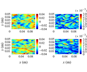
Figure 9 shows instantaneous maps of downwind velocity fluctuation,  $u^{\prime }$, and molecular scalar flux,
 $\unicode[STIX]{x1D705}\;\unicode[STIX]{x2202}C/\unicode[STIX]{x2202}z$, at the surface in LES-A at
 $t=4.63~\text{s}$ and at
 $t=7.41~\text{s}$. Figure 9(a,b) shows that the downwind velocity fluctuation at the surface is characterized by downwind-elongated positive streaks or high-speed streaks serving to locally enhance the downwind current. Note that the positive streaks generally coincide with the small-scale downwelling limbs and associated small-scale (filament) ejections of scalar observed in figures 7 and 8. In other words, the small-scale downwelling limbs and associated scalar ejections are generally located underneath the positive streaks of
 $u^{\prime }$.
Surface downwind velocity fluctuations ( $\text{m}~\text{s}^{-1}$) at (a)
 $t=4.63~\text{s}$ and (b)
 $t=7.41~\text{s}$, and (c,d) corresponding scalar concentration fields (
 $\text{mol}~\text{m}^{-3}$) in LES-A.

Figure 9(c,d) shows that the molecular diffusive scalar flux at the surface is characterized by low-flux streaks coinciding with the positive streaks in  $u^{\prime }$ in figure 9(a,b). At
 $t=4.63~\text{s}$, a characteristic spacing between low-flux streaks (i.e. positive
 $u^{\prime }$ streaks) is seen to be
 $l=0.01~\text{m}$. The corresponding spacing in dimensionless viscous length units is
 $l^{+}=lu_{\unicode[STIX]{x1D70F}}^{w}/\unicode[STIX]{x1D708}_{w}=87$. At
 $t=7.41~\text{s}$, the spacing is greater with a characteristic value of about
 $l^{+}=130$. These spacings are close to the spacing of 100 between low-speed wall streaks in classical wall-bounded, shear-dominated turbulence reported by Smith & Metzler (Reference Smith and Metzler1983). A similar spacing was observed between low-flux streaks in the DNS of Takagaki et al. (Reference Takagaki, Kurose, Tsujimoto, Komori and Takahashi2015).
Figures 10–12 present the previously described turbulent structures corresponding to LES-B. Comparing figures 10–11 with 7–8, it can be seen that in LES-B the development of centimetre-scale LC is more prominent with coherent limbs extending closer to the surface and engulfing the small-scale eddy activity (e.g. see two leftmost downward-pointing arrows in figure 11a). In LES-B the centimetre-scale LC is also seen to extend deeper into the water column than in LES-A. Furthermore, during a simulation time of about 6.5 s, in LES-B, the larger LC scales can grow to occupy the entire spanwise extent of the domain, as can be seen through the single upward-pointing arrow and the single downward-pointing arrow in figures 11(c) and 11(d). This is in contrast with figure 8(c,d) showing that in LES-A, the largest LC does not grow as fast, with the spanwise extent of the domain able to capture two pairs of centimetre-scale LC. The development of larger centimetre-scale LC in LES-B than in LES-A is attributed to the Stokes drift shear extending deeper into the water column in LES-B than in LES-A, as can be seen in figure 4(b).
Cross-sectional (crosswind–vertical,  $y$–
 $z$) distributions of (a) instantaneous and (c) downwind-averaged vertical velocity fluctuations (
 $\text{m}~\text{s}^{-1}$), and (b,d) corresponding scalar concentration fields (
 $\text{mol}~\text{m}^{-3}$) in LES-B at
 $t=4.44~\text{s}$. The crosswind–vertical distributions in (a,b) are shown at the
 $x$ location halfway along the streamwise length of the domain.

Cross-sectional (crosswind–vertical,  $y$–
 $z$) distributions of (a) instantaneous and (c) downwind-averaged vertical velocity fluctuations (
 $\text{m}~\text{s}^{-1}$), and (b,d) corresponding scalar concentration fields (
 $\text{mol}~\text{m}^{-3}$) in LES-B at
 $t=6.48~\text{s}$. The crosswind–vertical distributions in (a,b) are shown at the
 $x$ location halfway along the streamwise length of the domain.

Surface downwind velocity fluctuations ( $\text{m}~\text{s}^{-1}$) at (a)
 $t=4.44~\text{s}$ and (b)
 $t=6.48~\text{s}$, and (c,d) corresponding scalar concentration fields (
 $\text{mol}~\text{m}^{-3}$) in LES-B.

Comparing figures 9 and 12, it can be seen that the downwind-elongated streaks of positive  $u^{\prime }$ and corresponding downwind-elongated streaks of low scalar flux are coarser in LES-B than in LES-A. This can be attributed to the lower surface Stokes drift shear in LES-B, evidence of the impact of the waves on the small-scale turbulence structure at the surface.
In figures 12(b) and 12(d), it can be seen that in LES-B, by  $t=6.48~\text{s}$ the positive
 $u^{\prime }$ streaks and corresponding low-flux streaks have conglomerated in the region
 $y<0.03~\text{m}$. This corresponds to the fact that the small-scale surface eddy activity has conglomerated along the top of the single downwelling limb of the centimetre-scale LC captured by the domain. This single downwelling limb can be seen occupying the region
 $y<0.03~\text{m}$ in figures 11(a) and 11(c).
As noted earlier, the behaviour of the small-scale ejections conglomerating above larger-scale downwelling limbs is also observed in the DNS of Takagaki et al. (Reference Takagaki, Kurose, Tsujimoto, Komori and Takahashi2015). Furthermore, this conglomerating behaviour is consistent with field observations of Langmuir turbulence. As noted by Leibovich (Reference Leibovich1983), in Langmuir turbulence ‘the small scales continually form and are slowly swept up into the more permanent larger scales’.
Overall, the small-scale surface eddy activity described above for LES-A and LES-B possesses similarities with the small-scale motions in classical wall-bounded shear-driven turbulent boundary layers, for example, in terms of their corresponding low-speed streaks and their spacing. As such, this small-scale turbulence has been considered distinct from the larger centimetre-scale LC motions by Takagaki et al. (Reference Takagaki, Kurose, Tsujimoto, Komori and Takahashi2015). However, given the observations above, specifically the coalescing of bursting small-scale motions engendering larger-scale motions and ultimately the centimetre-scale LC, as well as the correspondence between conglomerating small-scale surface eddy activity and associated surface streaks and the small-scale and large-scale Langmuir motions noted by Leibovich (Reference Leibovich1983), here the small-scale bursting eddy activity at the surface is interpreted as part of the LC scale range and thus part of the Langmuir turbulence regime. Furthermore, note that the small-scale bursting motions in the LES have been triggered by the combined effect of the wind and waves through the C–L vortex force (LES-A, LES-B and LES-C) as these motions and the overall turbulence are absent in the LES without the C–L vortex force (LES-D).
3.2.3 Lumley invariants and turbulence structure
In order to further investigate the turbulent structure, we consider the Lumley invariants of the anisotropy tensor defined as
 $$\begin{eqnarray}\displaystyle \unicode[STIX]{x1D623}_{ij}=\frac{\langle u_{i}^{\prime }u_{j}^{\prime }\rangle }{2q}-\frac{\unicode[STIX]{x1D6FF}_{ij}}{3}, & & \displaystyle\end{eqnarray}$$
where  $\langle u_{i}^{\prime }u_{j}^{\prime }\rangle$ is the instantaneous resolved Reynolds stress tensor with the angle brackets denoting averaging over
 $x$ and
 $y$ and with
 $u_{1}^{\prime }=u^{\prime }$,
 $u_{2}^{\prime }=v^{\prime }$ and
 $u_{3}^{\prime }=w^{\prime }$. Furthermore,
 $q$ is the instantaneous resolved turbulent kinetic energy defined earlier and
 $\unicode[STIX]{x1D6FF}_{ij}$ is Kronecker’s delta. In particular, the map of the square root of the second invariant (
 $II=\unicode[STIX]{x1D623}_{ij}\unicode[STIX]{x1D623}_{ji}$) versus the cube root of the third invariant (
 $III=\unicode[STIX]{x1D623}_{ij}\unicode[STIX]{x1D623}_{jk}\unicode[STIX]{x1D623}_{ki}$) should lie inside the so-called Lumley triangle for a realizable turbulent flow (see figure 13 for the shape of the Lumley triangle). Furthermore, the location of the map inside of the triangle corresponds to the structure of the turbulence. For example, if the map falls close to the right-hand edge of the triangle, the turbulence is cigar-shaped. An example of this type is shear-dominated turbulence in which the streamwise component of the velocity fluctuations is dominant over the other two components. If the map falls closer to the left-hand edge of the triangle, the turbulence corresponds to two-component turbulence such as stably stratified turbulence in which the horizontal components of the velocity fluctuations dominate over the vertical component. The uppermost vertex of the triangle, the lowermost vertex and the left-hand vertex correspond to one-component turbulence, three-component isotropic turbulence and two-component isotropic turbulence, respectively.
Depth trajectories of the second and third Lumley invariants in the upper third portion of the water column. The solid arrow points to the map at the surface of the water column ( $z=0.025~\text{m}$) and the dashed arrow points to the map at
 $z=0.018~\text{m}$.

Figure 13 plots the Lumley invariant map  $(III^{1/3},II^{1/2})$ at depths in the upper-third portion of the water column for LES-A and LES-B at various times after transition to turbulence had occurred. It can be seen that regardless of the state of the small-scale motions and the centimetre-scale LC, the trajectories of the Lumley invariant maps for LES-A and B consistently move from the right-hand edge of the triangle towards the interior and left-hand vertex with decreasing distance from the surface. Thus, the turbulence may be considered two-component in the upper-third portion of the water column approaching nearly two-component isotropic at the surface. This two-component structure is due to elevated near-surface crosswind velocity fluctuations which together with strong downwind velocity fluctuations serve to dominate over the vertical velocity fluctuations. This structure is characteristic of Langmuir turbulence near the surface observed in previous LC computational studies of Tejada-Martínez & Grosch (Reference Tejada-Martínez and Grosch2007) and field studies of Gargett & Wells (Reference Gargett and Wells2007). This result further supports the conclusion reached earlier that the small-scale surface turbulence is part of the Langmuir turbulence regime.
3.2.4 Vertical scalar flux
The impact of the centimetre-scale LC and near-surface small-scale motions on scalar flux throughout the water column is investigated through figure 14. This figure plots instantaneous depth profiles of the molecular diffusive scalar flux,  $\unicode[STIX]{x1D705}\;\text{d}\langle C\rangle /\text{d}z$, and the resolved turbulent vertical flux of the scalar,
 $-\langle C^{\prime }w^{\prime }\rangle$, in LES-A and LES-B. Recall that the angle bracket notation denotes averaging over horizontal directions
 $x$ and
 $y$. Following Akan et al. (Reference Akan, Tejada-Martínez, Grosch and Martinat2013), the contribution of the larger LC scales resolved (corresponding to centimetre-scale LC) to
 $-\langle C^{\prime }w^{\prime }\rangle$ may be defined as
 $-\langle \langle C^{\prime }\rangle _{x}\langle w^{\prime }\rangle _{x}\rangle$. This contribution is also plotted in figure 14 for the LES-A and LES-B cases. In the previous expression, the notation
 $\langle \cdot \rangle _{x}$ denotes averaging in the streamwise direction.
Depth profiles of the components of the resolved total vertical flux of the scalar concentration ( $\text{mol}~\text{m}^{-2}~\text{s}^{-1}$): molecular diffusive flux,
 $\unicode[STIX]{x1D705}\;\text{d}\langle C\rangle /\text{d}z$ (solid), resolved turbulent flux,
 $-\langle C^{\prime }w^{\prime }\rangle$ (dashed), and contribution of centimetre-scale LC to the the resolved turbulent flux,
 $-\langle \langle C^{\prime }\rangle _{x}\langle w^{\prime }\rangle _{x}\rangle$ (dash-dotted).

In figure 14, it can be seen that in both LES-A and LES-B, the scalar is distributed to greater depths with time as the centimetre-scale LC grows and becomes more coherent.
In figure 14, as expected, the molecular diffusive flux decays rapidly with depth given the strong vertical mixing present in all cases. In all cases shown in figure 14, in the near-surface region at  $z\sim 0.024~\text{m}$ (corresponding to a distance
 $z^{+}=8.7$ from the surface which is just outside of the viscous sublayer for which
 $z^{+}<5$), the molecular diffusive flux is negligible and the turbulent scalar flux
 $-\langle C^{\prime }w^{\prime }\rangle$ is nearly equal to the molecular diffusive scalar flux at the surface. In LES-A at
 $t=4.63~\text{s}$ (figure 14a) at
 $z=0.024~\text{m}$, the turbulent scalar flux is 88 % larger than the viscous scalar flux. Furthermore in LES-A at
 $t=4.63~\text{s}$, at
 $z=0.024~\text{m}$, the contribution from the centimetre-scale (larger-scale) LC to the total turbulent flux is 15 %. By
 $t=7.41~\text{s}$ (figure 14b), although the contribution from the centimetre-scale LC to the total turbulent flux is now 25 %, this contribution is still small. In LES-B (figure 14c,d) the contribution of the centimetre-scale LC at
 $z=0.024~\text{m}$ to the turbulent flux is greater than in LES-A. This is expected, given that in LES-B the larger scales become more predominant (coherent) with time, as shown earlier. However, note that in LES-B the wind and wave forcing parameters (i.e.
 $La_{t}$ and
 $\unicode[STIX]{x1D706}$) were idealized variations of the realistic
 $La_{t}$ and
 $\unicode[STIX]{x1D706}$ values chosen for LES-A, as discussed in § 3.2. Overall, in the more realistic LES-A case the contribution from the centimetre-scale LC is small, and thus it may be concluded that the smaller-scale turbulence (smaller than the centimetre-scale LC) contributes the bulk of the flux, thereby strongly influencing the gradient of the scalar concentration at the surface and the corresponding molecular diffusive scalar flux at the surface. This conclusion is in agreement with the conclusion reached by Takagaki et al. (Reference Takagaki, Kurose, Tsujimoto, Komori and Takahashi2015) from their DNS that the smaller-scale turbulence controls the scalar flux across the air–water interface.
Finally, it should be mentioned that the contribution of centimetre-scale LC to a fluctuation such as  $w^{\prime }$ has been computed by Takagaki et al. (Reference Takagaki, Kurose, Tsujimoto, Komori and Takahashi2015) as
 $w_{LC}^{\prime }=\widehat{\langle w^{\prime }\rangle _{x}}$. In this expression, the hat notation
 $\hat{\cdot }$ denotes application of a low-pass filter along the crosswind direction
 $y$ with filter width set to the characteristic distance between downwelling limbs of the centimetre-scale LC. Meanwhile, in the present work, the contribution by centimetre-scale LC has been computed as
 $w_{LC}^{\prime }=\langle w^{\prime }\rangle _{x}$, i.e. without the application of the low-pass filter. The difference between these two approaches for computing
 $w_{LC}^{\prime }$ is interpreted as follows. If the low-pass filter is taken as the spectral cut-off filter such that the filtered field retains the largest Fourier mode associated with LC, then
 $w_{LC}^{\prime }=\widehat{\langle w^{\prime }\rangle _{x}}$ represents the largest LC scale (singular) present. In contrast,
 $w_{LC}^{\prime }=\langle w^{\prime }\rangle _{x}$ represents the largest LC scales (plural) present, corresponding to a multiple of the largest Fourier modes.
Computation of the contribution of centimetre-scale LC to  $-\langle C^{\prime }w^{\prime }\rangle$ as
 $-\langle \widehat{\langle C^{\prime }\rangle _{x}}\widehat{\langle w^{\prime }\rangle _{x}}\rangle$ (not shown) leads to the same trends observed in figure 14 and thus the same conclusions reached above for which the centimetre-scale LC contribution was computed as
 $-\langle \langle C^{\prime }\rangle _{x}\langle w^{\prime }\rangle _{x}\rangle$.
4 Conclusion
Large-eddy simulations of a wind- and wave-driven shear flow were conducted to investigate the structure of LC and associated Langmuir turbulence resulting from the interaction between the wind-driven shear and the Stokes drift induced by wind-driven gravity–capillary waves. Simulation results were also analysed to understand turbulent scalar transport and turbulence-enhanced molecular diffusive scalar flux at the surface. Wave–current interaction generating the LC was represented through the C–L vortex force consisting of the cross-product between the inputted Stokes drift velocity and the flow vorticity. Simulations started from near rest with the sudden imposition of the C–L vortex force and a wind stress corresponding to a  $5~\text{m}~\text{s}^{-1}$ wind speed.
The LES with the C–L vortex force showed good agreement with previous DNS of coupled air–water boundary layers with deforming air–water interface characterized by gravity–capillary waves (Komori et al. Reference Komori, Kurose, Iwano, Ukai and Suzuki2010; Takagaki et al. Reference Takagaki, Kurose, Tsujimoto, Komori and Takahashi2015; Hafsi et al. Reference Hafsi, Tejada-Martínez and Veron2017). The good correlation was seen in terms of (1) downwind-elongated streaks characterizing the downwind velocity fluctuations and the molecular diffusive scalar flux at the water surface, (2) the near-surface turbulent scalar transport characterized by intermittent ejections of high-concentration fluid from the surface by small-scale bursting motions, (3) the growth of centimetre-scale LC emanating from small-scale eddy activity at the surface and (4) the spike in molecular diffusive scalar flux at the surface induced by transition to turbulence and subsequent relaxation to a statistically steady-state value.
Various cases, namely LES-A, LES-B and LES-C (with different wave parameters (amplitude and wavelength) in the C–L vortex force and with the same wind stress as the DNS), were simulated in order to investigate the influence of the wave forcing on the turbulence and scalar transport. It was seen that surface Stokes drift shear combined with the wind-driven shear through the C–L vortex force are responsible for triggering turbulence serving to enhance molecular diffusive scalar flux at the surface with respect to a simulation without C–L vortex forcing which did not transition to turbulence. The enhancement is independent of the wave parameters implying that it is only a function of wind shear (wind speed). Features of the small-scale turbulence triggered are similar to the classical shear-driven turbulence next to a wall characterized by so-called high- and low-speed, streamwise-elongated ‘wall streaks’ with the high-speed streaks corresponding to bursting motions emanating from the wall or the rigid-lid surface in the present case. Initially, bursting motions emanating from the surface coalesce to form larger scales with the growth and coherency of these scales controlled by the Stokes drift shear. A Stokes drift shear extending deeper into the water column, such as in LES-B, promotes the rapid development of larger, more coherent motions, i.e. centimetre-scale LC, fed by the small scales at the surface as these scales conglomerate at the top of the downwelling limbs of the larger-scale motions. A shallower Stokes drift shear, such as in LES-A, promotes the same process but at a slower rate. The range of eddies in this process starting from the small-scale bursting motions at the surface through the larger, coherent centimetre-scale LC is categorized as Langmuir turbulence and is consistent with field observations of this turbulence regime described by Leibovich (Reference Leibovich1983).
Control of the near-surface turbulent scalar transport and the molecular diffusive scalar flux at the surface is shared between larger-scale motions and the smaller-scale surface activity. Initially, the smaller-scale bursting motions tend to control the near-surface scalar transport and the molecular scalar flux at the surface. As time progresses and the larger-scale motions become more prominent, greater control is transferred to these scales, although their influence on the molecular scalar flux at the surface remains small compared to that of the smaller scales. The transfer of control depends on the Stokes drift shear, as Stokes drift shear extending deeper into the water column tends to drive faster formation of coherent larger scales and faster transfer of control to these scales. Regardless of this partitioning of control, and thus regardless of the wave parameters determining the Stokes drift shear depth profile, the intensity of the surface turbulence scales with the wind-driven shear, i.e. the wind speed. Thus, it is concluded that the Langmuir turbulence and the scalar flux induced at the surface by the Langmuir turbulence scale with the wind speed. This result explains why the scalar flux across the air–water interface reaches a statistically steady value despite growing, wind-driven gravity–capillary waves in previous DNS of coupled air–water molecular boundary layers.
The independence of the turbulence intensity and thus the molecular diffusive scalar flux at the surface from wave parameters could potentially be a low-Reynolds-number effect. Akan et al. (Reference Akan, Tejada-Martínez, Grosch and Martinat2013) has shown that increasing Stokes drift shear at the surface enhances the small-scale turbulence at the surface and ultimately the flux at the surface in wind- and wave-driven flows at Reynolds number approximately twice the Reynolds number simulated here. Recall that the Reynolds number of the wind- and wave-driven water flows in the present study was  $Re_{\unicode[STIX]{x1D70F}}^{w}=217$ based on wind stress friction velocity and vertical length of the water domain. The flows of Akan et al. (Reference Akan, Tejada-Martínez, Grosch and Martinat2013) were simulated in a shallow-water column setting where the Langmuir cells engulf the entire water column and interact with the bottom boundary layer. Furthermore, the results of Akan et al. (Reference Akan, Tejada-Martínez, Grosch and Martinat2013) were obtained with the turbulence under statistical equilibrium and thus the transition of the flows to turbulence was not explored.
Small-scale LC occurs frequently in lakes and lagoons. As noted by Veron & Melville (Reference Veron and Melville2001), in the ocean, large gravity waves and breaking waves will tend to disrupt the gravity–capillary wave field, and thus small-scale LC is not expected often. In the DNS and LES presented in the paper as well as in physical experiments of Veron & Melville (Reference Veron and Melville2001), inception of small-scale LC accompanied by transition to Langmuir turbulence caused a spike in scalar flux characterized by an order-of-magnitude increase. These flux increases, if linked to episodic gusts and unsteadiness in the wind field, are expected to be an important contributor in determining the long-term average of the air–water fluxes in lakes and lagoons. Thus, future research should exploit DNS and LES to develop improved parameterizations of scalar transfer during transition to Langmuir turbulence across different wind speeds (Reynolds numbers).
Acknowledgements
This work was supported in part through US National Science Foundation grants 1235039 and 1233808 to A.E.T.-M. and F.V., respectively. A.H. also acknowledges support from a Sloan Foundation fellowship.



