1. INTRODUCTION
In an effort to model long-run economic relationships, a large literature on cointegration has developed, starting with the seminal work of Granger (1981) and Engle and Granger (1987). One branch of this literature pertains to finding the number of cointegrating relations, that is, the cointegrating rank of the underlying system. For that purpose, various statistics have been proposed, with the likelihood ratio (LR) tests of Johansen (1988, 1991) being widely used. The latter are based on estimating a vector autoregression of the form (omitting deterministic components)

Under the assumption of Gaussian errors and known lag order, the LR tests for the hypothesis that Π has rank, say, r are constructed using the technique of reduced rank regression involving the solution to an eigenvalue problem (see Anderson, 1951). The asymptotic distributions of the tests, again assuming known lag order, are derived by Johansen (1988, 1996) and Ahn and Reinsel (1990). These are nonstandard distributions that can be expressed in terms of Brownian motions (and also deterministic components, if they are included in the regression).
In practice, the lag order k is unknown and needs to be chosen prior to constructing the tests. Many studies have shown by simulations that the tests may suffer from serious size distortions if the lag order is not chosen appropriately; see, for example, Cheung and Lai (1993), Yap and Reinsel (1995), and Lütkepohl and Saikkonen (1999). To this end, it has been proposed to use information criteria such as Akaike's information criterion (AIC) (Akaike, 1973) and the Bayesian information criterion (BIC) proposed by Schwarz (1978). Lütkepohl and Saikkonen (1999) provide some theoretical and simulation evidence in support of such a proposal. They show that the AIC and the BIC are asymptotically valid criteria in the sense that the resulting cointegration tests will have the same limiting distributions as if the lag order is finite and known.
Recently, there also has been increased interest in extending the analysis of cointegrated systems beyond the finite-order vector autoregressive (VAR) case. Yap and Reinsel (1995) consider testing for cointegration in a vector autoregressive moving average model (VARMA) under the assumption that the orders for the AR and MA components are known a priori. Lütkepohl and Saikkonen (1997) study the analysis of impulse response functions in infinite-order VAR processes. Kuersteiner (2005) extends the analysis of Ng and Perron (1995) to prove the validity of a general-to-specific testing strategy to select the vector autoregression order when the process is a strictly stationary infinite-order VAR model and the goal is to get coefficient estimates that are consistent and asymptotically normal.
More closely related to our work is the paper by Saikkonen (1992), who considers estimating and testing for cointegration using a finite VAR approximation when the true process is an infinite-order vector autoregression. Saikkonen and Luukkonen (1997) justify the use of Johansen's LR tests for cointegration for such processes and give sufficient conditions on the lag order, under which the associated tests have the same limiting distributions as in the finite-order case. In this context, choosing a lag order amounts to finding a good enough approximation to the true data generating process (DGP) to yield a cointegration test that has an exact size close to nominal size while retaining acceptable power. Simulation results by Lütkepohl and Saikkonen (1999), and others presented in this paper, show that the use of the AIC or BIC leads to tests with unacceptable size distortions. The problem is particularly serious when the noise component has a moving average (MA) representation with a root close to one, in which case the lag lengths chosen by the AIC and the BIC are too small, resulting in poor approximations to the true process and consequently in tests with substantial size distortions. As shown subsequently, this can also occur in a finite VAR system when the coefficients of the last few lags are small but have nevertheless an important effect on the overall correlation structure of the series. Because it is important to have a reliable procedure that yields tests with acceptable size and power, it is important to find a useful alternative to traditional information criteria for selecting the lag order.
In this paper, we extend the work of Ng and Perron (2001), who proposed a modified Akaike's information criterion (MAIC) in the context of choosing the autoregressive lag order to construct unit root tests. The main idea underlying their procedure is to use the information specified by the null hypothesis, as it relates to restrictions on the parameters of the model, to keep an extra term in the penalty function of the AIC. We show that this strategy leads to the following simple MAIC in the context of testing for cointegration using an LR test based on a VAR approximation:

where

is an estimate of the covariance matrix of et, N = T − KT − 1, with KT the maximal lag order allowed, and the extra term τk(r), relative to the AIC, is simply the LR test of r against more than r cointegrating vectors. It permits an overall penalty function that better represents the cost associated with an increase in the lag order. Simulations show that when the true order is infinite, or when the true order is finite but there is a weak correlation for the last lags, this extra term is highly sensitive to changes in the lag order and implies a selected lag higher than that obtained with a standard AIC. This leads to drastic improvements in the exact size of the cointegration tests with little loss in power. The MAIC, via the extra term τk(r), also adapts to the cointegration rank, the dimension of the system, and the nature of the deterministic components in the data and the regression.
We provide theoretical justifications for its validity, showing that the resulting cointegration tests have the same limiting distributions as when the lag order is finite and known. We also give simulation evidence showing that, compared with the AIC and the BIC, the resulting procedure yields drastic size improvements while preserving the power of the test.
The idea of using sample-dependent quantities in the penalty factor of an information criterion is not new. For instance, Phillips and Ploberger (1994) used a Bayesian approach to suggest the Posterior Information Criterion (PIC), whose penalty depends, in particular, on the second moment matrix of the regressors [see also the Fisher Information Criterion (FIC) of Wei, 1992; for a discussion of PIC in cointegration context see Phillips, 1996; Chao and Phillips, 1999]. But the motivation and performance are very different. The PIC and FIC allow different penalty parameters associated with stationary, integrated, or trending regressors. When performing unit root tests, these information criteria still yield tests that have high size distortions in the presence of a negative MA component (see Phillips and Ploberger, 1994, Table 2). The motivation behind the statistic that we incorporate in the penalty term is very different and directly motivated by the testing problem under consideration. We work under the null hypothesis of some cointegrating rank, and the aim is to have the penalty term adapt to the nature of the serial correlation present. In this sense, our MAIC is tailored to work for the problem of testing for cointegration and is unlikely to be suitable for other problems such as the selection of a model for forecasting purposes, in which case the PIC and FIC are likely to perform better. Also note that our approach involves a mix of information criteria and traditional LR testing procedures and hence is not immune to the problem of postmodel selection bias; see Leeb and Pötscher (2005).
The structure of the paper is as follows. Section 2 presents the models and cointegration test considered. Section 3 derives the exact form of the MAIC, stated earlier, in the context of a finite-order vector autoregression and illustrates its performance with one specific example. Section 4 shows its validity in the general case of a linear process having an infinite VAR representation and shows that cointegration tests constructed from a VAR approximation with a lag order selected by the MAIC have the same limit distribution as when the order is finite and known. The analysis also includes extensions to cover the case where various types of deterministic components are included. Section 5 studies the properties of the MAIC in a local asymptotic framework whereby the MA root is local to one, which explains why it provides an improvement over the traditional AIC when the true process is of infinite order. Section 6 presents simulations to show how, in such a case, the use of the MAIC yields tests with improved finite-sample properties, compared to what can be achieved using the AIC or BIC. Section 7 offers brief concluding remarks and an Appendix some technical derivations.
2. PRELIMINARIES
Let yt = (y1,t,…, yn,t)′ be an n-vector of time series variables available for t = 1,…,T. The cointegration test of Johansen (1988, 1991) is based on a VAR(k) approximation of the form

Under the hypothesis of r cointegrating vectors, the matrix Π has reduced rank, such that Π = αβ′ where α is an n × r matrix of adjustment coefficients and β is an n × r matrix whose columns contain the cointegrating vectors. In the literature, three cases are usually considered with respect to the nature of the deterministic components. These are


For Case A, no deterministic component is present, for Case B the constant is restricted, and for Case C, the constant is unrestricted and allows trend in the I(1) series.1
Perron and Campbell (1993) consider the case where an unrestricted time trend is also included in the model. Because this case is less often used in practice, we shall not provide explicit results for it, though the MIC to be derived is still applicable.
The construction of the test is based on an eigenvalue problem. Let R0t be the residuals from a regression of Δyt on (Δyt−1,…, Δyt−k) and R1t be the residuals from a regression of yt−1 on (Δyt−1,…, Δyt−k). For Case B, the dependent variable is (1,yt−1) in the construction of R1t, and for Case C, a constant is added to the list of regressors. Define

and let

be the n − r smallest eigenvalues of the system |λS11 − S10 S00−1S01| = 0. To test the null hypothesis of r cointegrating vectors versus the alternative that there are more than r cointegrating vectors, Johansen's trace statistic
2Throughout this paper, we consider the so-called trace test. Note, however, that everything remains valid when considering the maximal eigenvalue test, for which the alternative hypothesis is that the cointegrating rank is r + 1.

where N = T − k − 1 denotes the sample size used for estimation, k is the lag order, and γδ is the number of parameters associated with the deterministic components. Johansen (1988, 1991) derived the limit distribution of the LR test assuming a known finite order k. Saikkonen and Luukkonen (1997) extended the analysis to show that the same limit distribution applies when the data are generated by a general linear process of weak dependence, in which case the true autoregressive order is infinite. This will be the case if the order k of the VAR approximation is chosen in such a way that it increases to infinity as the sample size increases but at a controlled rate (less than T1/3); see also Lütkepohl and Saikkonen (1999). They recommend the use of an information criterion to select k, such as the BIC or AIC.
In economic applications, a nonfinite true autoregressive order is often the result of an MA component in the VARMA representation of the system. Such cases are indeed relevant in practice. For example, suppose that some component of the system yi,t is the sum of a random walk and a white noise measurement error; then Δyi,t is an MA(1) process with a negative MA coefficient. In practice, the log of aggregate output is often modeled as an unobserved component autoregressive moving average (ARMA) model, consisting of a stochastic trend that accounts for the long-term growth and a stationary component that represents the cycle. This implies an equivalent ARMA representation for the first difference of yi,t. Of related interest, Yap and Reinsel (1995) consider a system of three U.S. monthly interest rate series and argue that it can be modeled as a VARMA(1,1) process with the largest (in absolute value) MA root being −0.40. In principle, it is possible to test for cointegration using a VARMA process directly (Yap and Reinsel, 1995). However, in the presence of a negative MA component, estimates such as those based on maximum likelihood can have finite-sample properties that make them difficult to assess (e.g., the issue of multiple local optima and the so-called pile-up problem). Hence, it is often simpler and more reliable to adopt a vector autoregression, which is easy to estimate and, as we shall see, yields tests with good properties provided the lag length is selected appropriately.
To illustrate the potential pitfalls of using an information criterion to select the lag length in the context of a system containing an MA component, we present the size of the LR test from a simple simulation exercise (see also Lütkepohl and Saikkonen, 1999). Consider a bivariate process with no cointegration, that is,

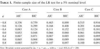
where Δyt = (Δy1,t,Δy2,t)′, εt ∼ i.i.d. N(0,I2), and y0 = ε0 = 0. The sample size is T = 200, and the number of replications is 10,000. The LR test is constructed from a VAR(k) approximation with k selected using either the BIC or the AIC restricting the search to values of k between 0 and KT = int(12(T/100)1/4), which is often employed in practice. The experiments are repeated for various values of φ between −0.8 and 0.8. To evaluate the size of the LR test we use the appropriate asymptotic critical values corresponding to Cases A–C, for tests with 5% nominal size. The results are presented in Table 1. First, they clearly show that serious size distortions exist when a large negative MA root is present. In the case of a large positive MA root, size distortions also exist, though they are not as serious. Second, using the BIC implies tests with substantially worse properties than if the AIC is used, given that the former imposes a stronger penalty that results in a smaller order being selected. Third, the tests show more severe size distortions when more deterministic components are included in the estimated system. This is particularly relevant in practice because most economic variables contain a nonzero mean or a trend.
Finite-sample size of the LR test for a 5% nominal level

With this background information, the rest of the paper is devoted to the derivation of an alternative information criterion following the work of Ng and Perron (2001), which allows tests with finite-sample size close to nominal size, and this with little loss of power.
3. THE MODIFIED AKAIKE'S INFORMATION CRITERION
To derive the form of the modified information criterion (MIC) we shall start by assuming that the data are generated by a finite-order vector autoregression with independent and identically distributed (i.i.d.) normal innovations, and we will subsequently analyze its large-sample properties in a more general context. We also abstract from deterministic components in both the DGP and the estimated system. As discussed in Ng and Perron (2005), when selecting the lag order, it is important to estimate each candidate model with the same numbers of effective observations. Given the fact that variations in the order k imply different numbers of initial conditions, this means that all candidate models are estimated with N = T − KT − 1 observations, where KT is the maximal value that defines the range over which k can be a candidate, the lower bound being zero. So the model used for the n-vector yt is

for t = KT + 2,…,T, where et ∼ i.i.d. N(0,Σ). Under the null hypothesis that the cointegrating rank of the system is r, we have Π = αβ′ as defined earlier. To facilitate the derivations, it is useful to adopt a reparameterization of the model. Define wt = (Δyt−1′,…, Δyt−k′)′ and Γ = (Γ1,…,Γk); then (6) is equivalent to

where we note that yt−1 is I(1), an integrated process of order one, and wt is I(0) in the sense that its partial sums satisfy a functional central limit theorem (FCLT). In what follows we shall simply refer to these components as the nonstationary and stationary components. Following Anderson (1951), we project yt−1 onto the range space of wt and define yt−1* and Γ* by

and we can write (6) as

which is useful because the regressors yt−1* and wt are orthogonal. Finally, define Ψ = (Π,Γ*), θ = (Ψ,Σ), and xt−1 = (yt−1*′,wt′)′; (6) can then be equivalently represented as

The aim of an information criterion in this context is to select the order k of the VAR approximation. We shall for now assume that the true order of the preceding model is k0 and a model of order k ≥ k0 is estimated. This is a strong assumption, and it is done to simplify the derivation. The same technique is commonly used in other studies, for example, Linhart and Zucchini (1986, p. 245) and Hurvich and Tsai (1989). We use this assumption for Sections 3.1 and 3.2 when deriving the MIC. In Section 4, we relax it and allow for the case where the approximating family does not include the true model.
Hence, the log-likelihood function conditional on the first KT + 1 observations is

with θ = (Ψ,Σ) the parameters of the model.
3.1. General Observations on the Construction of Akaike's Information Criterion
In this section, we briefly discuss the principles underlying the derivation of the AIC. For a detailed discussion, the readers are referred to Akaike (1973, 1974), Cavanaugh (1997), and Burnham and Anderson (1998, pp. 43–50). See also the paper by Shibata (1980), who shows that the AIC asymptotically minimizes the mean squared error for the estimation of the parameters and also the integrated mean squared error for the estimation of the spectral density when the underlying model is a stationary Gaussian autoregression with infinite order. Pötscher (1989) studies its property when applied to a nonstationary autoregressive model, while assuming the true process is of finite order.
The treatment follows Cavanaugh (1997), with slightly different notations. Suppose we have the observed data y = (y1,…, yT) whose log-likelihood function is l(y;θ). Let θ0 denote the true values of the parameters.
3Note that both θ0 and θ depend on k. This dependence is, however, not explicitly stated to simplify the notation.

. Also, because we do not wish the result to apply conditional on the particular sample available, we shall consider a process yF, with the same distribution as y but generated by a different history for the innovations, and shall average over such possible processes. Hence, the aim is to maximize

Akaike's information criterion is then a quantity, say, AIC, whose expectation is twice the function to be minimized (aside from an error of order o(1)), that is,

To proceed further, consider the following decomposition of the objective function:

For term (I), because k ≥ k0, we can apply a second-order Taylor expansion around

, with an error term of order op(1), that is,

where the first-order term equals zero because the score is zero when evaluated at the MLE. The second equality follows because yt−1*′ and wt′ are orthogonal. We again apply a second-order Taylor expansion to term (II), this time around the true value of the coefficients, so that

where again the first-order term is zero because the expected score is evaluated at the true values of the coefficients and the second equality follows because yt−1*′ and wt′ are orthogonal. The traditional derivation of the AIC proceeds as follows. First, we have the following result:

because each quantity converges to the same chi-square random variable with kn2 degrees of freedom given that wt is a stationary process. Second, because k ≥ k0,

say, where

are different random variables (because, with yt−1* a nonstationary process, the limit of

is a random variable, unlike the case with stationary regressors), which are functions of a vector Wiener process and the cointegrating rank. The important thing is that they do not depend on k. Hence,

, and an asymptotically unbiased estimate of

(aside from an error of order o(1)) is given by

and a quantity AIC such that E0(AIC) has the same value (again aside from an error of order o(1)) is

which reduces to

, and maximizing this quantity is equivalent to minimizing the traditional

.
The crucial point to make here is that, even though the term A defined by (8) does not depend on k in large samples, it is highly dependent on this lag order in finite samples, and approximating it by a constant may give a distorted picture of the adequate penalty to be imposed on additional lags. Following the main idea proposed by Ng and Perron (2001), we note that the null hypothesis specifies some structure on the parameters of the matrix Π, in particular its rank, as specified by the number of cointegrating vectors. The idea is then to use this information to replace the constant C by a random variable that, in the limit, has the same expected value as A provided k ≥ k0 (up to a constant to be made precise later) and, hence, satisfies the principles underlying the construction of the AIC. The resulting quantity is dependent on k in finite samples in such a way as to better account for the quality of the competing models as approximations to the true process.
3.2. An Alternative Approximation for the Term A
We now provide an alternative approximation for the term A that uses the information on the parameters imposed by the null hypothesis of a cointegrating rank r. We start by separating the process yt* into two parts: a stationary component and a nonstationary noncointegrated component. More specifically, because the cointegration rank of yt, and hence that of yt*, is r, there exists an invertible matrix P, with Q = P−1, such that (see Reinsel, 1993, p. 166) Q(In + Π)P = diag[In−r,Λr] = J, where J is the Jordan canonical form. Hence, we have

where P = [P1,P2], Q′ = [Q1,Q2], with P1 and Q1 n × (n − r) matrices, so that z1t* = Q1′yt* is nonstationary and noncointegrated and z2t* = Q2′yt* is stationary (again in the sense that it is an I(0) process whose partial sum satisfies a FCLT). Also, ΠP1 = 0, and, equivalently, if Π = αβ′, then β′P1 = 0 because α is of full rank. Define the scaling matrix

with the first block corresponding to z1t* and the second to z2t*. Then, using these results,

where ζ1,rn asymptotically has a chi-square distribution with rn degrees of freedom. The last equality follows because the matrix

is asymptotically block diagonal. The second block corresponds to the r stationary elements and, hence, has the usual chi-square limit distribution. Consider now the term A2. Using similar arguments and the fact that the limit of

is the same as that of

(because the series are stationary), we have

Now let

The limit of φrn is a function of Wiener processes and the underlying parameters of the model. The important thing is that it does not depend on k provided k ≥ k0 (Reinsel, 1993, p. 167). The term A2 can then be written as

Collecting terms, we have

We now impose the null hypothesis that Π0 = α0 β0′, and because these are unknown, we replace them with the MLE obtained assuming the reduced rank structure, denoted

. This induces a difference to A whose limit distribution again does not depend on k provided k ≥ k0. Hence, a quantity with the same expected value in large samples as A (up to a constant that does not depend on k provided k ≥ k0) is

The preceding quantity, which is discussed in detail by Reinsel (1993), is asymptotically equivalent to twice the LR test for testing the null hypothesis of r cointegrating vectors as analyzed by Johansen (1991), which we denote by4
The appropriate notation should be τT,k(r), but we shall omit the dependence on T for simplification.

The corresponding MAIC, substituting the constant C in (9) by 2τk(r), is then

The extra term in the penalty function of the MAIC is closely related to that derived by Ng and Perron (2001) in the univariate context, and the reasons why it yields improvements are similar. In Ng and Perron (2001), this extra term was related to a unit root test based on an autoregression and involved the sum of the autoregressive coefficients. In their case, the bias in the sum of the autoregressive coefficients is dependent on the order of the autoregression; especially when the MA polynomial has a root close to one. Their simulations show that this bias decreases as the order increases, thereby reducing the overall penalty. Because this bias flattens out as the autoregressive order increases, the overall shape of the penalty function is nonlinear. The same explanation applies here except that, in this multivariate context, the unit root test is replaced by the cointegration test and Π is the equivalent of the sum of the autoregressive coefficients, being a function of the sum of the coefficient matrices of the VAR polynomial.
More generally, we can consider a class of information criteria of the form

If CT = 2, we have the MAIC, if CT = ln ln N, we may call it the modified Hannan–Quinn criterion (Hannan and Quinn, 1979), and if CT = ln N, we have a modified BIC. As for the traditional class of information criteria, we can specify a class of MIC with CT either constant or such that CT → ∞ and CT /T → 0 as T → ∞. We will analyze the MIC at this level of generality in the next sections.
The MIC takes a simple form and is very easy to apply. Consider the problem of testing r against more than r cointegrating vectors. First, we need to choose an upper bound KT, and the following vector autoregression needs to be estimated for 0 ≤ k ≤ KT:

where deterministic components may be included depending on the underlying process. For each case, we need to construct the following two quantities:

where N = T − KT − 1 and

are estimated residuals from (11). Note that a possible choice of the upper bound is KT = int(12(T/100)1/4), which is used by Ng and Perron (2001). Also, when constructing (12) no finite-sample adjustment is applied; the scaling used follows from the likelihood principle we have adopted.
5The aim of the finite-sample adjustment is to have a statistic whose asymptotic distribution is a better approximation to the exact distribution. Here, such a concern is not present because the use of the test is to make the penalty factor better approximate the relevant penalty to be applied for the testing procedure.
It is important to emphasize that the extra term in the MIC provides only a finite-sample adjustment. Asymptotically the MIC and the standard information criteria described are equivalent. Hence, to provide a theoretical explanation of why the extra term allows significant improvements in the exact size of the cointegration tests would require asymptotic expansions, which in this context are very complex and outside the scope of our analysis. Instead, we shall offer explanations for some special cases of interest using theoretical arguments and simulations. In a first step, we consider how the MIC can offer improvements even in finite-order vector autoregressions (see Section 3.3), a fact overlooked by Ng and Perron (2001). In a second step, we consider the behavior of the MIC when the process is an MA of order one. In this case, we can provide theoretical explanations using a local asymptotic framework. This is done in Section 5 and complemented with simulation results in Section 6.
3.3. Size Improvement in Finite-Order VAR Models
We here consider how the MAIC can offer an improvement over traditional information criteria when the process is a finite-order vector autoregression. We work with the following simple example of a VAR(3) given by

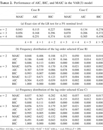
where yt is an n-vector with n = 2, 3, and 4, T = 200, εt ∼ i.i.d. N(0,In) for t > 0, and εt = 0 for t ≤ 0. An important feature of this process is that there is fairly weak correlation at lags 2 and 3 but that jointly they account for a substantial portion of the overall correlation because the first coefficient is also fairly small. To show the relative size properties of the MAIC, BIC, and AIC, we generated data according to the models given by equations (2) and (3) (the results for the model in equation (1) are similar and are not reported). All results are obtained using 10,000 replications. The exact sizes for the test with a 5% nominal size are reported in Table 2, part (a). It is clear that the use of the AIC and the BIC results in size distortions that increase with the dimension of the system and the number of deterministic components. On the other hand, the MAIC offers significant improvements, yielding exact sizes close to the 5% nominal level.
Performance of AIC, BIC, and MAIC in the VAR(3) model

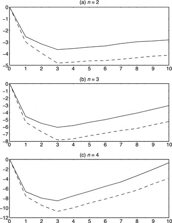
To better understand the role of the extra term τk(r) in allowing for tests with better exact sizes, we report in Figure 1 the median (over all replications) of τk(0) − τ0(0) as a function of k. There are several features worthy of note. First, the penalty term is decreasing until k = 3 (the true value), at which point it reaches a minimum, and there is also a further (less important) increase as k increases beyond 3. This nonlinear effect acts in a way to penalize any value of k different than 3. Second, the extent of the decrease is more important for the model in equation (3) than for the model in equation (2), which means that τk(r) also adapts to the nature of the deterministic components in the estimated system. Third, the decrease is also more important the larger the number of variables n in the system. These last two features explain why the MAIC is able to bring the exact size close to nominal size in all cases even though the size distortions implied by the use of the AIC or BIC are higher the larger the number of variables in the system or the number of deterministic components in the estimated regressions.

τk(0) − τ0(0) as a function of k: VAR(3), T = 200 (solid line: Case B; dashed line: Case C).
To see how the presence of the extra penalty term τk(r) affects the lag order selected, Table 2 presents the frequency distributions of the lag order selected by the MAIC, AIC, and BIC. The results show that the BIC selects 0 lag almost 100% of the time. The AIC selects either 0 or 1 lag most of the time. On the other hand, the MAIC selects 0 lags with small probability and higher order lags more often than the BIC or AIC. Note that the fact that the MAIC does not select 3 lags with the highest probability is not a defect and is because the MAIC adapts to the actual correlation in a particular sample. Indeed, unreported simulations showed that the exact size of the cointegration test using the MAIC is as good as when using a fixed number of lags set at the true value 3.
4. LAG ORDER SELECTION IN A GENERAL VAR MODEL WITH REDUCED RANK STRUCTURE
We now study the property of the MIC in a general framework. Following Lütkepohl and Saikkonen (1999), we consider the following DGP:

where u1,t and u2,t are r × 1 and (n − r) × 1 vectors, respectively, and ut = [u1,t′,u2,t′]′ is a weakly stationary process. The system is assumed to have a triangular structure without loss of generality, because the MIC and other statistics considered later are invariant to a rotation of the system. Also, it is assumed that the system contains no deterministic component, which will be relaxed later. The system may also be written as

where vt = [v1,t′,v2,t′]′ is a linear transformation of ut given by

We assume that the process {vt} has the following representation:

with {Gj}j=0∞ and {εt}t=1∞ satisfying the following conditions.
Assumption 1. The matrices {Gj}j=0∞ are a sequence of constants satisfying G0 = In and

for some a > 1; {εt}t=1∞ is an i.i.d. sequence with var(εt) = Σ and E(∥εt∥4) < ∞.
6We use the assumptions of Lütkepohl and Saikkonen (1999) because we shall appeal to many of their results. We conjecture that the conditions can be relaxed, in particular to allow for conditional heteroskedasticity, as in, for example, Phillips and Solo (1992) and Chang and Park (2002). Such an extension is, however, outside the scope of our paper.
This assumption imposes mild restrictions on the temporal dependence of vt, which are satisfied by a large family of processes, for example, all stationary and invertible ARMA processes with i.i.d. innovations. However, it excludes processes with long-range dependence. Note that if Gj = 0 for j > k0, then vt is a finite-order VAR(k0) process. Assumption 1 also implies that the process yt can be approximated by the following finite-order vector autoregression:

with

The difference between εt and et goes to zero if k → ∞. In other words, the process Δyt can be approximated arbitrarily well by an AR(k) process by choosing a large enough k.
Because the process is cointegrated of rank r, Π has reduced rank, and we now specify it with the following triangular structure, without loss of generality:

with Φ an n × r matrix of full column rank and Θ′ = [Ir : −A]. To study the properties of the lag order selected by the MIC, denoted kMIC, and its effect on the limit distribution of the cointegration test, we need to specify a maximum order allowed, KT. We use the same assumption as in Ng and Perron (2001) and Lütkepohl and Saikkonen (1997):
Assumption 2. The order kMIC is selected from a set of values of k ranging from 0 to KT, with KT chosen such that KT → ∞ and KT3/T → 0, as T → ∞.
We now study the property of the MIC when the data are generated by (14). We need the following lemma, which is concerned with the behavior of τk(r) when the lag length k varies between 0 and KT.
LEMMA 1. Suppose the data are generated by (14) with cointegrating rank r and let τ(r) denote the limiting distribution of the LR test when the true order is finite and known. Then, under Assumptions 1 and 2,
(i) if vt is a VAR process of order k0, τk(r) →d τ(r) uniformly in k0 ≤ k ≤ KT and τk(r) = Op(1) uniformly in 0 ≤ k < k0;
(ii) if vt is an infinite-order vector autoregression, τk(r) →d τ(r) holds for any sequence of k satisfying k → ∞ and k ≤ KT. Also, τk(r) = Op(1) uniformly in 0 ≤ k ≤ M for any M < ∞.
The next result is concerned with the lag order selected by the MIC when the data are generated by a finite-order VAR process, that is, Gj = 0 for j > k0 in (15). It establishes that the MIC has the same properties as the usual information criteria, namely, that the lag order is consistently estimated if CT → ∞ and CT /T → 0 as the sample size increases and that when CT is fixed, the probability of underestimation is zero in large samples.
PROPOSITION 1. Suppose the data are generated by (14) with vt a VAR process of order k0. Also assume the cointegrating rank is r. Then, under Assumptions 1 and 2,
(i) if CT is a constant, Pr(kMIC ≥ k0) → 1, as T → ∞;
(ii) if CT → ∞ with CT /T → 0 as T → ∞,

.
The next result is concerned with the lag order selected by the MIC when the process is an infinite-order vector autoregression.
PROPOSITION 2. Suppose the data are generated by (14) with vt an infinite-order VAR process. Also assume that the cointegrating rank is r. Then, under Assumptions 1 and 2, kMIC → ∞ in probability, as T → ∞.
The proof follows directly from the proof of Proposition 1 in the Appendix, and hence the details are omitted. The next result states that the LR test for cointegration constructed from a vector autoregression whose order is selected by the MIC has the same limit distribution as when the order is finite and known.
PROPOSITION 3. Suppose the data are generated by (14) and assume that the cointegrating rank is r. Then, under Assumptions 1 and 2, the LR test for cointegration, constructed from a vector autoregression whose order is selected by the MIC, has the same limit distribution as when the order is finite and known.
For the proof of Proposition 3, the reader is referred to Theorem 5.2 of Lütkepohl and Saikkonen (1999). The details are omitted.
4.1. Model with Deterministic Components
The DGP (14) assumes that the process contains no deterministic component. In practice, it is often important to consider processes with a nonzero mean or a linear trend. More precisely, suppose the data are generated by

where u1,t and u2,t are as specified previously. We consider the following three possibilities with respect to the data and the regression system used.
Case 1. The DGP contains an intercept but no trend (δ2 = 0), and the regression system includes a restricted constant, that is, equation (2).
Case 2. The DGP contains a linear trend (δ2 ≠ 0, i.e., at least one variable is trending), and the regression system includes an unrestricted constant, that is, equation (3).
Case 3. The DGP contains an intercept but no trend (δ2 = 0), and the regression system includes an unrestricted constant, that is, equation (3).
The following proposition establishes that our results carry through in these cases.
PROPOSITION 4. If the data are generated by (19) with Cases 1–3 applying, then the results of Propositions 1–3 continue to hold.
To prove this proposition, the key is to establish the appropriate parameterization of the regression. The proof involves finding the limiting distribution of the inverse of the moment matrix of the regressors. If linear trends are present and Case 2 applies, asymptotically this moment matrix may not have full rank because of the fact that the linear trends dominate and hence the inverse is not well behaved. For example, consider a bivariate unit root process yt = (y1,t, y2,t)′ with y1,t and y2,t having a common linear trend; then the moment matrix of yt is asymptotically of rank 1, after rescaling. This difficulty can be solved using an equivalent parameterization for the regression (see, e.g., Hamilton, 1994, p. 627), which yields a block diagonal matrix of full rank when suitably rescaled. Here, we outline how this is achieved for Case 2. The detailed proof is in the Appendix. Let

and

and suppose that the elements of y2,t are ordered such that E(Δy2,t(n)) = δ2(n) ≠ 0, that is, y2,t(n) contains a linear trend. Then, the fitted values from the regression system (3) are equivalent to those obtained with the following regression system:

where

and Δyt−jd = Δyt−j − δ,

, Π* = [Π1,…, Πn−1]. In (20), yt−1d contains no trend, Δyt−jd is mean zero, and only y2,t(n) contains a linear trend. Hence, the moment matrix of the regressors is asymptotically block diagonal, and the inverse is Op(1) when appropriately scaled. With this, the proof proceeds as in Lütkepohl and Saikkonen (1999).
Note that when studying the properties of the cointegration tests when the AIC is used, Lütkepohl and Saikkonen (1999) only consider processes with no deterministic trend and conclude that the analysis with trending variables is a nontrivial task. Our results thereby also establish that their conclusions continue to apply with trending variables. In spite of their asymptotic validity, we will show in the next sections that their performance is substantially inferior to that of the MIC in the context of infinite-order VAR processes.
In practice, to apply the MIC the nature of the deterministic components needs to be specified a priori. This is different from Phillips (1996), where the cointegration rank, lag length, and trend degree are determined jointly and where the approach and motivation differ from the present paper, as discussed earlier.
5. THE BEHAVIOR OF τk(r) UNDER A LOCAL ASYMPTOTIC FRAMEWORK
This section examines the behavior of τk(r) under a local asymptotic framework similar to that used in Ng and Perron (2001), which provides a theoretical explanation for the key difference in the finite-sample properties of lag orders selected using the MIC or a standard information criterion when a negative MA component is present. As discussed earlier, τk(r) will influence the choice of k when there is a large negative MA root, a situation for which cointegration tests such as Johansen's LR test exhibit severe size distortions. To understand the issue of lag length selection in this setting, a useful device is to use an asymptotic framework in which the MA coefficients are parameterized as local to −1. So we consider the following process:

where y1,t and y2,t are of dimensions r and n − r, respectively, and

with u1,t and εt i.i.d. sequences with finite fourth-order moments and c > 0 is a constant. We also suppose that

As T increases to infinity, θT → −1, and y2,t becomes a white noise process. However, y2,t is an integrated process that is nearly white noise in finite samples. Nabeya and Perron (1994) used this asymptotic framework to derive an approximation to the finite-sample distribution of the least-squares estimator in a first-order autoregressive model with negative MA errors and showed this approximation not only to be superior to those obtained from standard asymptotic distributions but also to be quite accurate even for small sample sizes. Perron and Ng (1996) used the same setup to analyze the size and power of various unit root tests based upon autoregressions. Our aim here is to use the same device to obtain useful qualitative features about the relative properties of the information criterion and MIC. The results are presented next.
PROPOSITION 5. Let the data be generated by (21); then under Assumption 2, as T → ∞,
(i) for any fixed k, the limiting distribution of τk(r) is unbounded;
(ii) for any sequence of k satisfying k → ∞ as T → ∞ and k4/T → 0,

where W(s) is an (n − r)-dimensional vector Wiener process.
Proposition 5 extends the result of Theorem 2 in Ng and Perron (2001) to the multivariate case.7
We conjecture, similar to the analysis of Ng and Perron (2001) in the univariate case, that it would be possible to show, using this local asymptotic framework, that setting CT to a constant is optimal. This requires, however, the derivations of asymptotic expansions, which are very complex in our multivariate framework and beyond the scope of this paper.
6. SIMULATIONS OF THE FINITE-SAMPLE PROPERTIES
We now conduct simulations to assess the finite-sample properties of the lag order selected by the MAIC and the implied size and power of the LR test for cointegration. In the simulations, the lower bound of the order is always zero and the upper bound is KT = int(12(T/100)1/4). All results are obtained using 10,000 replications. We consider only the case where an unrestricted constant is included in the regression, that is, regression (3). The reason is that the size distortions of the cointegration test are highest in this case, and we will clearly show that even in this worst case our method is able to deliver tests with sizes very close to nominal level (the results for the other cases are similar).
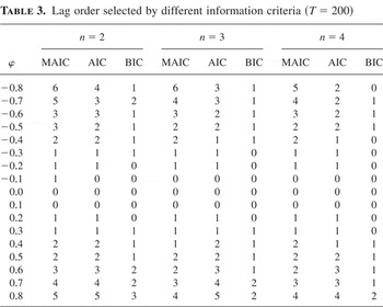
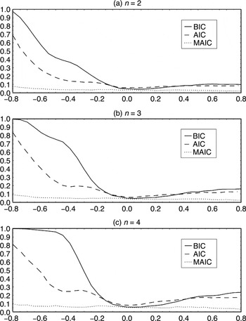
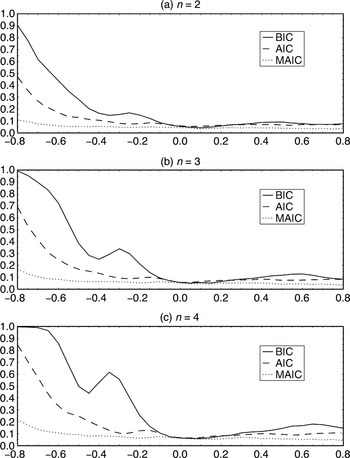
We use the DGP (5) considered in Section 2 and report results for systems of dimensions n = 2,3, and 4. Consider first the simulations pertaining to the lag orders selected by the MAIC, the BIC, and the AIC. The median (over all replications) of the lag selected is reported in Table 3 for a sample of size T = 200. The results clearly show that the MAIC selects a lag order that is greater than that selected by the AIC or BIC, especially when the MA coefficient is large and negative. As expected, when the correlation is small all information criteria agree to select a small order. To investigate the implications of these differences, we now turn to the exact size of the LR cointegration test when a 5% nominal size is used. We present results for T = 100 and 200 in Figures 2 and 3, respectively. These show not only that the use of the MAIC permits dramatic improvements over the use of either the AIC or BIC, but also that the exact size is nearly 5% over the entire parameter space.
Lag order selected by different information criteria (T = 200)


Exact size of Johansen's LR test for r = 0 (5% nominal level, T = 100).

Exact size of Johansen's LR test for r = 0 (5% nominal level, T = 200).
It is also interesting to investigate the exact size when r > 0.8
We thank a referee for suggesting the following simulation experiment.

where u1,t and u2,t satisfy

and

Also, y1,0 = ε1,0 = y2,0 = ε2,0 = 0. We consider the size of the LR test for r = 1 at the 5% nominal level with T = 200. We are interested in the effects of (θ1,θ2,ρ) on the size, and accordingly four configurations of parameters are considered:
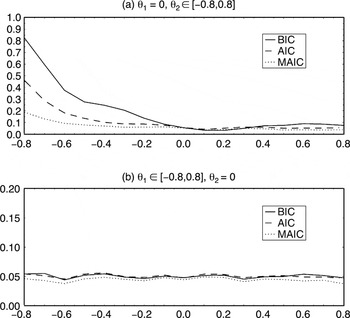
- θ1 = ρ = 0, θ2 varies between −0.8 and 0.8.
- θ1 varies between −0.8 and 0.8, θ2 = ρ = 0.
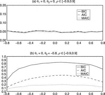
- θ1 = θ2 = 0, ρ varies between −0.9 and 0.9.
- θ1 = 0,θ2 = −0.8, ρ varies between −0.9 and 0.9.
The first parameterization allows an MA component in the stochastic trend, although not in the equilibrium errors. The results are presented in Figure 4a, which again confirms our finding that the MAIC is able to bring the exact size close to the nominal size, whereas using the AIC and the BIC results in serious size distortions. The second parameterization allows an MA component in the equilibrium errors but not in the stochastic trend. Not surprisingly, as shown in Figure 4b, size distortions do not occur, and the three criteria perform equally well.

Exact size of Johansen's LR test for r = 1; uncorrelated shocks (5% nominal level, T = 200, n = 2).
The last two parameterizations examine the effect of cross-equations correlation. To better isolate its effect, we first set θ1 = θ2 = 0. The results are presented in Figure 5a, which shows the information criteria to be robust to cross-equations correlation. We then introduce an MA component, and the picture now changes drastically, as shown in Figure 5b. Interestingly, a strong cross-equation correlation tends to offset the effect of the MA component. This is because when a strong correlation is present, y1,t − y2,t serves as a good proxy to ε2,t. Hence, the lagged values of y1,t and y2,t, as a subset of the regressors in the vector autoregression, can effectively reduce the serial correlation, which implies that a long lag is not needed to yield approximately uncorrelated residuals. This is also explained by Proposition 5, which shows that the magnitude of τk(r) is smaller when Σ21Σ11−1Σ12 is large. Overall, it is obvious that across all values of ρ ∈ [−0.9,0.9], the MAIC performs substantially better than the AIC and the BIC.

Exact size of Johansen's LR test for r = 1; correlated shocks (5% nominal level, T = 200, n = 2).
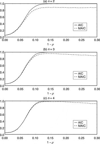
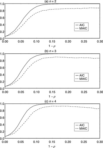
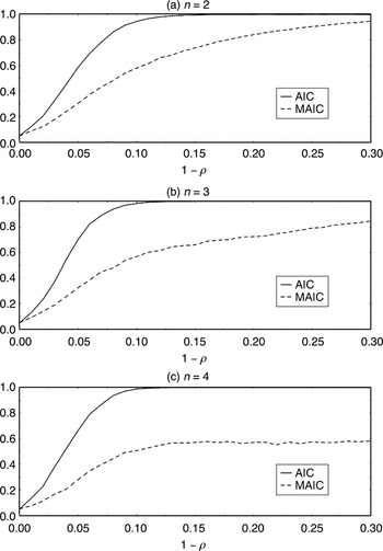
It remains to show that this improvement in the exact size of the cointegration test does not come at the expense of a substantial power loss. To that effect, we simulate the size-adjusted power of the test when the lag order is selected with the MAIC and the AIC. The DGP used is a simple stationary VARMA(1,1) given by

with εt ∼ i.i.d. N(0,In), y0 = ε0 = 0, and ρ varying between 1 and 0.7. Hence, under the alternative the cointegrating rank is n. The results are presented in Figures 6, 7, and 8 for θ = 0, −0.4, and −0.8. They show that there is virtually no power loss when the extent of the correlation is mild, that is, using the AIC or the MAIC leads to tests with the same properties when the extra term in the MAIC is not needed. There is some power loss when the MA component is very negative, which increases as the number of variables in the system increases. This seems a small price to pay to have an exact size close to nominal size. Unreported simulations show that when θ is positive or when the model includes less deterministic components, the power loss is smaller.

Size-adjusted power of Johansen's LR test for r = 0 (5% exact size, T = 200, θ = 0).

Size-adjusted power of Johansen's LR test for r = 0 (5% exact size, T = 200, θ = −0.4).

Size-adjusted power of Johansen's LR test for r = 0 (5% exact size, T = 200, θ = −0.8).
6.1. Simulations Calibrated to a Practical Case
Although the previous simulation exercise is useful to assess the general properties of the approximations, it remains to show how the approximations fare in the context of DGPs that are most likely to occur in practical applications. To that effect, we now consider a simulation design calibrated to the economic application considered by Yap and Reinsel (1995). It is a trivariate system with a VARMA(1,1) structure that is calibrated from a VAR model for three U.S. monthly interest rates.9
A similar configuration is used by Saikkonen and Luukkonen (1997) and Lütkepohl and Saikkonen (1999).

where C = P diag(λ1,λ2,λ3)Q − I3, Θ1 = Pθ diag(−λθ,0.297,−0.202)Qθ, with Q = P−1,Qθ = Pθ−1, and

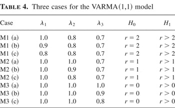
Note that the cointegrating rank is determined by the values of (λ1,λ2,λ3). We consider the same three cases as Yap and Reinsel (1995), which are shown in Table 4.
Three cases for the VARMA(1,1) model

Note that in each case the first row, (a), corresponds to a process satisfying the null hypothesis, and the second and third rows, (b) and (c), correspond to processes satisfying the alternative hypothesis. For each case, we compute Johansen's LR trace statistic from a regression system with a restricted constant, that is, equation (2). The sample size is set to T = 200.
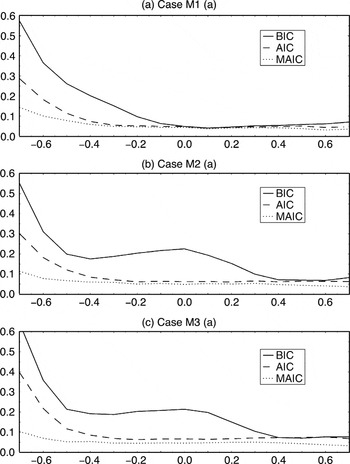
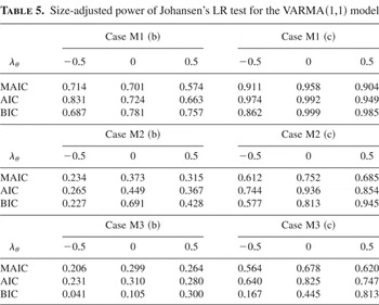
To examine the exact size, we let λθ vary between −0.7 and 0.7 and compute the empirical rejection frequencies for each λθ at the 5% nominal level. The rejection rates, as a function of λθ, are presented in Figure 9. Again, the results show that tests based on a VAR approximation with the order selected using the AIC or BIC exhibit severe size distortions. On the other hand, if the lag order is selected with the MAIC, the exact size of the test is close to 5% throughout the parameter space considered. Table 5 presents results for the size-adjusted power. Again, the use of the MAIC implies only a small loss of power relative to the AIC, and the test is more powerful than with the BIC for some configurations.

Exact size of Johansen's LR test with the empirically calibrated VARMA(1,1) model (nominal size 5%, T = 200).
Size-adjusted power of Johansen's LR test for the VARMA(1,1) model

7. CONCLUSIONS
We considered the properties of cointegration tests constructed from a VAR approximation when the data are generated by a general linear process of weak dependence. We showed that the BIC and AIC are not sufficiently flexible for cointegration tests, in that they lead to the selection of a model that is too parsimonious with the implication that the cointegration tests exhibit substantial size distortions, especially when a negative MA component is present. We extended the work of Ng and Perron (2001), who suggested a modification, the MAIC, which is evidently more robust when there are MA errors negatively correlated and with a finite VAR system when the coefficients of the last few lags are small but have nevertheless an important effect on the overall correlation structure of the series. The idea behind the derivation of the MAIC is to use information in the null hypothesis of the test, as it relates to restrictions on the parameters, to incorporate an extra term in the penalty function. Here, this extra term is simply the LR test for cointegration itself, and hence the procedure is indeed very easy to use in practice. The use of this MAIC to select the order of the VAR approximation leads to cointegration tests with exact sizes close to nominal size over, basically, the entire parameter space. It should therefore find wide appeal for practical applications. However, it should also be noted that although the suggested information criterion is useful in the context of cointegration tests, as we have shown, it may not be appropriate when selecting the lag order in other contexts, such as selecting a VAR approximation for the purpose of forecasting.
APPENDIX
Throughout this Appendix, we use the following notation. The euclidean norm of a matrix A is denoted by ∥A∥, with ∥A∥ = [tr(A′A)]1/2. The vector induced norm for A is denoted by ∥A∥1, with ∥A∥1 = supx≠0∥Ax∥/∥x∥. Note that ∥A∥1 is then equivalent to the square of the maximum eigenvalue of A′A and thus ∥A∥1 ≤ ∥A∥. The symbols

and ⇒ denote, respectively, convergence in probability and weak convergence under the Skorohod topology, and Op(·) and op(·) are the usual symbols for the order of convergence in probability. For a square matrix A, |A| denotes the determinant of A. Also, N = T − KT − 1 is the effective sample size. Assumptions 1 and 2 are assumed to hold throughout. Lütkepohl and Saikkonen (1999) is denoted as LS in this Appendix due to frequent reference.
Proof of Lemma 1. The first result of part (i) follows immediately from LS (pp. 195–197). To verify the second result, note that for a given k satisfying 0 ≤ k < k0, Saikkonen and Luukkonen (1997, pp. 113–116, proof of Thm. 3.1) implies τk(r) = Op(1). (Alternatively, we can follow the argument of Johansen (1996, pp. 158–159), which leads to the same result.) The order Op(1) is obviously uniform in k because k0 is finite. The intuition behind this result is that when k < k0, the eigenvalues corresponding to the cointegrating vectors are still consistently estimated and converge to the true value at rate T. Hence the LR test still has the same order under the null hypothesis, although the limiting distribution is no longer nuisance parameter free.
When the DGP is an infinite-order autoregressive process, then τk(r) →d τ(r), which again follows the proof of LS (pp. 195–197). They also established the uniformity, that is, that the convergence holds for any sequence of k satisfying k → ∞ and k ≤ KT. The second result holds following the same argument as in part (i). █
Proof of Proposition 1. We need the following multivariate extension of Lemma 4.2 of Ng and Perron (1995), due to LS.
LEMMA A.1 (LS, Lem. 5.1). Suppose the data are generated by (13), satisfying Assumption 1 and having cointegrating rank r. Denote the maximum likelihood estimate of Σ from the unrestricted model (16) as

and that from (16) imposing the restriction Πyt−1 = Φu1,t−1 as

; then, uniformly in k ≤ KT:

To prove Proposition 1, we first show that Pr(k ≥ k0) → 1 when either CT is constant or CT → ∞ with CT /T → 0 as T → ∞. First, note that after imposing the restriction Πyt−1 = Φu1,t−1, regression (16) only involves stationary regressors. From Lewis and Reinsel (1985), we have that, for any k < k0,

converges in probability to a positive definite matrix. Hence, using Lemma A.1,

also converges in probability to the same positive definite matrix. The difference in the penalty term is, using Lemma 1,

Hence, a k < k0 is never selected asymptotically, and Pr(k ≥ k0) → 1. To show part (ii), note that

uniformly in k0 < k ≤ KT (LS, pp. 193–194). Meanwhile, the penalty term satisfies

with the last equality following from Lemma 1, where it is shown that τk(r) − τk0(r) = op(1) uniformly in k0 ≤ k ≤ KT. Hence, the penalty term is positive with probability arbitrarily close to 1 for large T and is of higher order than

. This implies MIC(k) − MIC(k0) > 0 with probability 1 if CT → ∞, and also Pr(k ≤ k0) → 1, which proves the result, because we have shown that Pr(k ≥ k0) → 1 also. █
Proof of Proposition 4. We first establish some lemmas, which extend Lemmas A1–A4 of LS. The difference is that we allow linear trends, which the results of LS do not cover. Suppose the data are generated by (19) with δ2(n) ≠ 0. We can write (20) as

where

,

, and

are deviations from their sample means. Rearranging terms,

where Π2* = 0,γ* = 0, and

is an integrated process with zero mean. Define

,

, and pt = [qt′ : ht]′ and also Ξ = [Γ1,…, Γk : Γk+1,1], ϒ = [Π2* : γ*], and Λ = [Ξ : ϒ]. Then, (A.2) can be written as

Let

be the ordinary least squares estimate of Λ from (A.3). Define the scaling matrix DT = diag[N−1/2Ink+r,D2,T] with D2,T = diag[N−1In−r−1,N−3/2]. Finally, define the moment matrices

where Γqq = E(qt qt′), a nonrandom positive definite matrix. We use the partitions

and

. The following lemma characterizes the rate of convergence of the matrix

to R−1 and extends Lemma A1 of LS to the case with a linear trend.
LEMMA A.2. Suppose yt is generated by (19) with δ2(n) ≠ 0; then, as T → ∞, uniformly in k ≤ KT,
(i)

;
(ii)

;
(iii)

;
(iv)

;
(v)

.
Proof of Lemma A.2. We first show that the results hold for a given k ≤ KT. For part (i),

The first term is such that

using standard arguments as in Said and Dickey (1984) and the fact that the mean correction does not affect the order. For the second term,

follows from the property of integrated processes and the fact that

is asymptotically equivalent to a linear trend. Also,

, and hence the second term is of order Op((KT /N)) = op(1), which implies

. For part (ii),

Hence,

Part (iii) can be proved by changing the role of qt and ht and using similar arguments. For part (iv),

Part (v) follows automatically from parts (ii)–(iv). The remaining steps to establish that the results hold uniformly in k = O(KT) follow straightforwardly as in LS (p. 187). █
The next two lemmas extend Lemmas A2–A4 of LS to allow a linear trend in the DGP with variables replaced by deviations from their sample means. The intent is to show that we can impose the zero restrictions on the coefficients of the nonstationary regressors, ht, without affecting the asymptotic results. This essentially reduces the problem to that of a regression with only mean-zero stationary regressors, for which results have been established using a predictive regression framework, for example, Lewis and Reinsel (1985). We first need to define residuals from a predictive regression. Rewrite (A.3) as

where

and εtp is the one-step-ahead prediction error of the best linear predictor of Δyt based on qt. Because ϒ = 0, (A.4) can be augmented as

where Λp = [Ξp,ϒ] = [Ξp,0]. Denote the estimates of coefficients from (A.4) as

and the residual as

. Also, it is convenient to define (refer to (17))

and we have the following identity:

The next lemma extends Lemmas A2 and A3 of LS.
LEMMA A.3. Suppose yt is generated by (19) with δ2(n) ≠ 0; then, as T → ∞, we have, uniformly in k ≤ KT,
(i)

;
(ii)

;

;
(iii)

; in particular this term is op(1) if k → ∞.
Proof of Lemma A.3. We first show the results hold for a given k ≤ KT. For part (i),

For the first term, let y2,−1d denote the sample mean of y2,t−1d; then

where

is obtained using the definition of (y2,t−1d)′ (refer to (19)) and proceeding as in LS (pp. 187–188). Note that a similar result is also obtained by Said and Dickey (1984, p. 602). The result

follows by computing its variance, and ∥N−1/2(y2,−1d)′∥ = Op(1) is obtained by applying the FCLT. Similarly, we can show that the second term in (A.6) is op(1/k) using the fact that

behaves asymptotically as a linear trend. For part (ii), the first result follows from standard arguments as in Lewis and Reinsel (1985, p. 397), and the second follows from LS. The only difference is to note that the mean correction has no effect on the order of convergence. For part (iii), using (A.5), we have

The first term is op(1/k) by part (i), and for the second term

Using the result of LS (p. 191),

for some c < ∞, so that

because the vector

is of dimension O(k) and each is Op(1). Also,

by the same argument and the fact that

is dominated by the linear trend. Again, the completion of the proof to show that these results hold uniformly in k ≤ KT follows using the same arguments as in LS (p. 190). █
The following lemma pertains to the coefficient estimates from regression (A.2), extending Lemma A4 of LS. (Recall that

is the parameter estimate in the predictive regression (A.4).)
LEMMA A.4. Suppose that yt is generated by (19) with δ2(n) ≠ 0; then, as T → ∞, we have, uniformly in k ≤ KT,
(i)

;

;
(ii)

;

.
Proof of Lemma A.4. For part (i),

We have

by Lemma A.3(ii), and

; hence the first term is op(1). Also,

,

by Lemma A.3(iii), and

by Lemma A.1(iii). Hence the second term is Op(1). For part (ii), the second result follows directly from LS (p. 192). For the first,

The first term is op(KT /N) from LS (p. 192), whereas

which completes the proof. █
We are now in a position to prove Proposition 4. We only provide a proof for the case where the process contains a linear trend. The proof is similar to that in LS; hence we only outline the main differences and omit details. We first need to show that Lemma A.1 still holds, which can be shown using arguments as in LS (pp. 192–193), with the term corresponding to y2,t replaced by ht. Once this is done, the same proof as that of Proposition 1 can be used to show that the results of Propositions 1 and 2 hold when a linear trend is present. Then, with the preceding results, when the order is chosen by the MIC, we have
(a)

;
(b)

;
(c)

, where Φ is defined in (18) and

with J = [Ir,0]′;
(d)

.
These results can be proved by proceeding as in LS (pp. 194–197). Then, following the argument of Saikkonen and Luukkonen (1997, proof of Thm. 3.1), we can show that the LR test for r cointegrating vectors is asymptotically equivalent to the sum of the eigenvalues obtained as the solutions to the following system:

From results (a)–(d) asymptotically the solutions of the preceding problem coincide with those of

Hence, using the MIC leads to a cointegration test with the same asymptotic distribution as in the case with a finite and known lag order. █
Proof of Proposition 5. Recall that τk(r) is characterized by the following eigenvalue problem:

where

, with R0t the residuals from a regression of Δyt on (Δyt−1,…, Δyt−k) and R1t the residuals from a regression of yt−1 on the same set of regressors. Let the eigenvalues of the system (A.7) be

; then

To simplify notation, define wt = (Δyt−1′,…, Δyt−k′)′. We first establish a lemma that characterizes the distributions of the components of (A.7).
LEMMA A.5. Let W(s) be an n − r-dimensional vector Wiener process. If the data are generated by (21), then, under Assumption 2, as T → ∞ and uniformly in k,
(i)

.
(ii)

, with

Also, |V | = k + 1, and (V−1)1,1 = k/(k + 1).
(iii)

, with ι1 the k × 1 vector ι1 = (1,0,…,0)′.
(iv)

.
(v)

.
Proof of Lemma A.5. First, in what follows, all approximation results hold uniformly in k ≤ KT, unless stated otherwise. For part (i),

As in Nabeya and Perron (1994), y2,t can be decomposed as y2,t = aTεt + bT xt, with aT = −θT,

, and xt = xt−1 + εt, an integrated process of dimension n − r. Using a standard central limit theorem (CLT),

For the term

, we have

For the term

, we have

The preceding results imply that

For part (ii), by definition wt = [Δyt−1′,Δyt−2′,…, Δyt−k′]′; hence

is a kn × kn matrix, which can be partitioned into k2 blocks each of dimension n × n, where the (i,j) block of the partitioned matrix is

. We have the following results for different combinations of i and j. For i = j,

We have

using a standard CLT, and

where we have applied a CLT and a weak law of large numbers. Also,

Hence,

Applying similar arguments, we have, for i − j = ±1,

and for |i − j| > 1,

Hence,

where the difference is Op(k/T1/2) under the matrix norm. For part (iii), we consider the following two cases. For j = 1,

using the fact that y2t = aTεt + bT xt; and, for j ≥ 2,

Again, using a CLT and applying arguments similar to those in Lewis and Reinsel (1985) yields the desired result. Part (iv) follows from part (ii). Part (v) also follows directly. █
We now can proceed to prove Proposition 5. First, if k is fixed, all the eigenvalues of (A.7) are bounded away from zero. Accordingly τk(r) diverges at rate Op(T), which establishes the first result. For the second result, we first analyze the behavior of S10, S11, and S00 with k → ∞ and k4/T → 0. For S10,

using Lemma A5(ii)–(v). For S11,

using Lemma A5(i)–(iii). For S00,

using Lemma A5(ii) and (iv). Hence,

using the fact that S00 = Op(1). After some algebra, we can show that the r largest eigenvalues of (A.7) are of order Op(1/(k + 2)) and the others are of order Op(1/[(k + 1)(k + 2)]). To derive the limiting distribution of the smallest (n − r) eigenvalues, we follow the approach of Johansen (1996, p. 159). Define β = (Ir,0r×(n−r))′, β⊥ = (0(n−r)×r,In−r)′, and S(λ) = λS11 − S10 S00−1S01. Consider the decomposition

and let T → ∞ and λ → 0, such that ρ = (k + 1)(k + 2)λ is fixed. From (A.8)–(A.10),

Now,

again using (A.8)–(A.10). The preceding results imply that the smallest (n − r) eigenvalues, normalized by (k + 1)(k + 2), converge to those of

and the sum of the eigenvalues of (A.11) converges to

which completes the proof. █