3.1.1. Spectrum characteristics

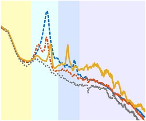
The power spectrum density for the noise of the plain cylinder and the corresponding background noise are presented in figure 6(a). Compared with the background, a sharp peak accompanied by one (at low Re) or two (at high Re) harmonic peaks abruptly appears in the spectrum as the cylinder is placed in the flow field, causing the sound pressure level (SPL) in space to soar dramatically. The dominant peak originating from vortex shedding is the Aeolian tone, i.e. the tonal noise, whose non-dimensional dominant frequency St ₀ (figure 6b) is the frequency of vortex shedding. The harmonic peaks are the second- and third-order harmonics of the Aeolian tone, whose frequencies are integer multiples of St ₀; for instance, when St ₀ = 0.18 at Re = 9.57 × 10⁴, the second and third harmonic frequencies are 0.35 (~2St ₀) and 0.53 (~3St ₀), respectively (the green spectrum in figure 6a). The spectrum characteristics of the plain cylinder in the present study agree well with the experimental results of Hutcheson & Brooks (Reference Hutcheson and Brooks2012), Geyer & Sarradj (Reference Geyer and Sarradj2016) and Kamps et al. (Reference Kamps, Geyer, Sarradj and Brücker2017). In figure 6(a), with an increase of Re, the SPL of the cylinder noise rises globally, whereas the non-dimensional frequency St ₀ of the Aeolian tone barely varies. All Re in the present experiment are included in the subcritical Reynolds number region, where St ₀ of the vortex shedding ranges from 0.180 to 0.191 according to the review by Norberg (Reference Norberg2003). As compared in table 2, St ₀ of the present experiment and those of previous investigations are in excellent agreement since the relative errors do not exceed 3 %, indicating that the measurement of St ₀ in the present experiment is reliable.

Figure 6.

(a) Power spectrum density for the noise of the plain cylinder. Solid line: cylinder noise, dashed line: background noise; red: Re = 3.83 × 10⁴, dark blue: Re = 5.74 × 10⁴, yellow: Re = 7.65 × 10⁴, green: Re = 9.57 × 10⁴; (b) definitions for the characteristic parameters of the Aeolian tone: the non-dimensional dominant frequency St ₀, the peak value SPL ₀, the first frequency f ₁ corresponding to (SPL ₀–10 dB), the second frequency f ₂ corresponding to (SPL ₀–10 dB) and the intensity of Aeolian tone I_A; (c) comparison of I_A between the results of Geyer & Sarradj (Reference Geyer and Sarradj2016) and the present experiment.

Table 2.

Comparison of St ₀ between results of previous studies and the present measurement.

The accuracy of the present measurement of the Aeolian tone is further verified by comparing the Aeolian tone intensity I_A of the plain cylinder in the experiment of Geyer & Sarradj (Reference Geyer and Sarradj2016) and the present study in figure 6(c); I_A is defined by the integral of the Aeolian tone in the power spectrum density (Geyer & Sarradj Reference Geyer and Sarradj2016), as shown in figure 6(b) and (3.1),

(3.1)\begin{equation}I_A = 10 \times \log _{10}{\displaystyle{\mathop \int \nolimits_{f_2}^{f_1} PSD({\hat{p}}^2)\,{\rm d}f} \over {p_{ref}^2 }}({\rm dB}),\end{equation}

where f ₁ and f ₂ are the first and the second frequencies corresponding to (SPL ₀–10 dB), respectively (figure 6b), and $PSD(\hat{p}^2)$ is the power spectrum density of the sound pressure; I_A is a crucial parameter in the analysis of the cylinder noise, which characterizes the overall intensity of the Aeolian tone induced by the vortex shedding. In the experiment of Geyer & Sarradj (Reference Geyer and Sarradj2016), the diameter and spanwise length of the circular cylinder model were D = 30 mm and L_S = 280 mm, respectively, and the noise was measured by a microphone located at (0, 500 mm, 0) (refer to the coordinate system in figures 1 and 2) over Re = 1.62 × 10⁴ ~ 10.60 × 10⁴. Although the spanwise length of the cylinder and the microphone location in Geyer & Sarradj (Reference Geyer and Sarradj2016) are different from those in the present study, the values of I_A at the monitor points of the two experiments are supposed to be roughly equal according to an empirical analysis with the theoretical model of the Aeolian tone, viz. (A3) in Appendix A. The specific derivation of the empirical analysis is provided in Appendix B. In figure 6(c), it is evident that the I_A–Re curve of the present experiment accords well with that of Geyer & Sarradj (Reference Geyer and Sarradj2016), and both of the two curves conform well to the Re ⁶ curve (refer to the (A3) in Appendix A), demonstrating that the measurement of I_A in the present experiment is reliable.

Figure 7 shows the noise spectra for the plain cylinder and the cylinder with the splitter plate for several representative cases. The splitter plate has a noticeable influence on the Aeolian tone and the high-frequency broadband noise. At a certain Re, e.g. Re = 5.74 × 10⁴ in figure 7(a–c), the Aeolian tone varies significantly with the increase of L/D. For L/D = 0.5 and 1.0, both the RSP and FSP effectively reduce the Aeolian tone, while the plates of L/D = 1.0 are more efficient than those of L/D = 0.5 (figures 7a and 7b). At L/D = 1.0, the peak value of the Aeolian tone (the SPL ₀ defined in figure 6b) for the plain cylinder and cylinders with RSP1.0 and FSP1.0 are $SPL_0^c = 84.01\;{\rm dB}$, $SPL_0^r = 68.68\;{\rm dB}$ and $SPL_0^f = 64.54\;{\rm dB}$ (figure 7b), respectively. These results manifest that an excellent noise reduction is achieved by RSP1.0 and FSP1.0; in addition, the SPL ₀ reduction by FSP1.0 (19 dB) is superior to that by RSP1.0 (15 dB). At L/D = 2.0, RSP2.0 aggravates the Aeolian tone with an SPL ₀ increment of 1.5 dB, whereas FSP2.0 still performs an effective reduction of approximately 10 dB (figure 7c). Besides, the St ₀ of the Aeolian tone is also altered by the splitter plates. At L/D = 1.0 and Re = 5.74 × 10⁴, St ₀ for the three case are $St_0^c = 0.192$, $St_0^r = 0.184$ and $St_0^f = 0.216$, respectively, i.e. RSP1.0 reduces St ₀ by 4.2 % while FSP1.0 increases St ₀ by 12.5 % (figure 7b). At L/D = 2.0, RSP1.0 and FSP1.0 increase St ₀ by 4.2 % and 16.7 %, respectively (figure 7c).

Figure 7.

Influence of L/D and Re on the power spectrum density of the cylinder noise: (a) Re = 5.74 × 10⁴, L/D = 0.5; (b) Re = 5.74 × 10⁴, L/D = 1.0; (c) Re = 5.74 × 10⁴, L/D = 2.0; (d) Re = 3.83 × 10⁴, L/D = 1.0.

At L/D = 1.0, compared with the plain cylinder, the spectrum for the cylinder with FSP1.0 exhibits an increase of noise by 8 ~ 10 dB in the high-frequency region and a rise of the second harmonic peak whose frequency St ≈ 2St ₀ (figure 7b). In contrast, there is no similar change in the spectrum of the cylinder with RSP1.0 (figures 7d). Figure 8 shows the difference between the PSD of the cylinder with and without the splitter plate, denoted as ΔSPL. In figure 8(a), ΔSPL = 8 ~ 10 dB for the cylinder with FSP1.0 for St > 0.3 characterizes the noise increment (the high-frequency region and the secondary peak) due to the installation of FSP1.0. The noise increase in the high-frequency region also occurred in the experiment of Kamps et al. (Reference Kamps, Geyer, Sarradj and Brücker2017), where the flow-induced noise of a circular cylinder was controlled by flexible hairy flaps made of eight flexible plates of L/D = 0.3. Their results illustrated that in the high-frequency region, f > 1000 Hz, the spectrum of the cylinder with hairy flaps increased by approximately 10 dB compared with the plain cylinder. Kamps et al. (Reference Kamps, Geyer, Sarradj and Brücker2017), however, did not give a definite elucidation for this phenomenon. In figures 7(c) and 8(b), at L/D = 2.0, the noise in the high-frequency region for both the cylinders with RSP2.0 and FSP2.0 somewhat increases. In the light of the numerical simulations of You et al. (Reference You, Choi, Choi and Kang1998) and Ali et al. (Reference Ali, Doolan and Wheatley2011) to control the cylinder noise with RSP, and the experiments of Chauhan et al. (Reference Chauhan, Dutta, More and Gandhi2018) and Sharma & Dutta (Reference Sharma and Dutta2020) to control the flow over a cylinder with RSP and FSP respectively, a small-scale but fairly strong trailing-edge vortex, viz. the secondary vortex named in the previous literature, occurred at the trailing edge of the splitter plate at L/D ≈ 2. Thus, it can be concluded speculatively but rationally that, in the present experiment, the increase of the high-frequency noise at L/D = 2.0 is induced by the interaction between the main vortices from the cylinder and the secondary vortex at the trailing edge of the splitter plate. This interaction increases the fluctuations with a high frequency in the flow field; accordingly, the corresponding noise in the high-frequency region increases. However, in terms of the phenomenon that FSP1.0 causes the increase of the high-frequency noise and the secondary peak, this is found by the present study for the first time, and no previous literature is available, which will be discussed in §§ 3.3 and 3.4.

Figure 8.

Spectra for ΔSPL, which is defined as the difference between the PSD of the cylinder with and without the splitter plate: (a) Re = 5.74 × 10⁴, L/D = 1.0; (b) Re = 5.74 × 10⁴, L/D = 2.0. The yellow regions denote the increment of noise in the high-frequency region and the secondary peak.

In figure 9, the reductions for the two splitter plates in the peak value of the Aeolian tone (SPL ₀) in the present experiment are compared with the results in Kamps et al. (Reference Kamps, Geyer, Sarradj and Brücker2017), Geyer & Sarradj (Reference Geyer and Sarradj2016) and Octavianty & Asai (Reference Octavianty and Asai2016). The reduction in SPL ₀ is evaluated by ΔSPL ₀, which is defined as the difference of SPL ₀ between the cylinder with and without control, i.e. $\Delta SPL_0 = SPL_0^{\; baseline} \; -\; SPL_0^{\; control} $. The data of previous studies in figure 9 are extracted from the spectra shown in the corresponding literature by the software GetData Graph Digitizer, and the extraction accuracy is approximately 0.1 dB pixel⁻¹. In the present study, RSP1.0 and FSP1.0 reduce the SPL ₀ by ΔSPL ₀ = 19 dB and 15.5 dB on average, respectively, and ΔSPL ₀ alters with Re hardly at all, meaning that their performances for the SPL ₀ reduction are stable, as shown by lines (b) and (d) in figure 9. By comparison, Kamps et al. (Reference Kamps, Geyer, Sarradj and Brücker2017) utilized the flexible hairy flaps to weaken the circular cylinder noise, and SPL ₀ was reduced by an average of ΔSPL ₀ = 20 dB for Re = 1.46 × 10⁴ ~ 3.4 × 10⁴ (line e in figure 9), which is slightly superior to the performance of FSP1.0 (ΔSPL ₀ = 19 dB) in the present experiment (line d in figure 9). Nonetheless, the performance of the hairy flaps for the SPL ₀ reduction is volatile, approaching the optimum stage with a reduction of ΔSPL ₀ = 24 dB at Re = 2.33 × 10⁴ and then declining progressively as Re increases (line e in figure 9). So, whether the hairy flaps can still reduce SPL ₀ by 20 dB on average in a higher Re range, for example Re = 4 × 10⁴ ~ 10⁵, remains to be verified experimentally. Moreover, Kamps et al. (Reference Kamps, Geyer, Sarradj and Brücker2017) also adopted fur that was attached to the rear of the circular cylinder for the noise reduction and accomplished an SPL ₀ reduction of ΔSPL ₀ = 16 dB on average (line f in figure 9), which is similar to the average reduction of ΔSPL ₀ = 15.5 dB for RSP1.0 in the present experiment (line b in figure 9). Geyer & Sarradj (Reference Geyer and Sarradj2016) controlled the circular cylinder noise over Re = 1.62 × 10⁴ ~ 10.60 × 10⁴ by means of surrounding the cylinder with several kinds of soft porous materials. Line (g) in figure 9 is the ΔSPL ₀–Re curve that belongs to the soft porous material named Panacell 90 ppi. Panacell 90 ppi produced the optimal SPL ₀ reduction of ΔSPL ₀ = 8–12 dB among all the materials used in Geyer & Sarradj (Reference Geyer and Sarradj2016), which is, however, inferior to the performance of FSP1.0 in the present experiment (line d in figure 9) and the hairy flaps in Kamps et al. (Reference Kamps, Geyer, Sarradj and Brücker2017) (line f in figure 9). Compared with the hairy flaps, the fur and the soft porous material, FSP1.0 is easier to implement in practice due to its simple structure, and its reduction in the cylinder noise is excellent. Hence, in terms of the reduction in the flow-induced noise of a circular cylinder, FSP1.0 is a compact device with high efficiency.

Figure 9.

Comparison of the reduction in the peak value of the Aeolian tone (SPL ₀) among Kamps et al. (Reference Kamps, Geyer, Sarradj and Brücker2017), Geyer & Sarradj (Reference Geyer and Sarradj2016), Octavianty & Asai (Reference Octavianty and Asai2016) and the present experiment, in which $\Delta SPL_0 = SPL_0^{\; baseline} -SPL_0^{\; control} $. Line (a–d): circular cylinder with RSP0.5, RSP1.0, FSP0.5 and FSP1.0, respectively, in the present experiment. Line (e) and line ( f): circular cylinder with hairy flaps that are made of eight FSPs with L/D = 0.3, and circular cylinder with fur that is glued using a large number of hairs with L/D = 0.5, respectively, in Kamps et al. (Reference Kamps, Geyer, Sarradj and Brücker2017). Line (g): circular cylinder surrounded by the soft porous material Panacell 90 ppi in Geyer & Sarradj (Reference Geyer and Sarradj2016). Point (h): square cylinder with a RSP of L/S = 0.5 (S is the side length of the square cylinder) in Octavianty & Asai (Reference Octavianty and Asai2016).

Octavianty & Asai (Reference Octavianty and Asai2016) controlled the noise from a square cylinder with RSP0.5 (a RSP of L/S = 0.5, where S denotes the side length of the square cylinder), and an SPL ₀ reduction of ΔSPL ₀ = 3.2 dB was obtained at Re = 3.3 × 10⁴, as presented by point (h) in figure 9. By contrast, at Re = 3.83 × 10⁴, both of RSP0.5 and FSP0.5 in the present experiment achieve an SPL ₀ reduction of ΔSPL ₀ ≈ 9 dB for the circular cylinder noise (lines a and c in figure 9). Thus, it is clear that the performance of the splitter plate in terms of the circular cylinder noise is considerably better than that for the square cylinder noise. This result further implies that the splitter plate may be more efficient in inhibiting the vortex shedding from a circular cylinder than that from a square cylinder. Interestingly, with the increase of Re, the performance of FSP0.5 for the SPL ₀ reduction steadily enhances (line c in figure 9), whereas that of RSP0.5 changes slightly (line a in figure 9). At Re = 9.57 × 10⁴, the performance of FSP0.5 resembles that of RSP1.0 (lines b and c in figure 9), where a ΔSPL ₀ ≈ 16 dB is yielded by both, which exceeds the ΔSPL ₀ = 9.6 dB of RSP0.5 at Re = 9.57 × 10⁴ significantly. When Re is low, FSP0.5 scarcely deforms and resembles a rigid plate, so its performance for the SPL ₀ reduction is similar to that of RSP0.5. In contrast, as Re increase gradually, the deformation and vibration of FSP0.5 are intensified; consequently, its performance for the SPL ₀ reduction enhances. This improved performance of FSP0.5 suggests that the movements of the FSP in the wake are conducive to the suppression of the vortex shedding and subsequently the Aeolian tone.

3.1.2. Characteristics of the Aeolian tone

Figures 10(a) and 10(b) illustrate the variations of I_A with L/D for the two splitter plates in the Re range 3.83 × 10⁴ ~ 9.57 × 10⁴. Figure 10(b) for the FSP only contains data in L/D = 0 ~ 3.0, because the FSP with L/D ≥ 4.0 vibrates violently with an excessive amplitude in the wake; meanwhile, a drastic resonance among the cylinder, the wind tunnel and the FSP itself is excited, preventing the subsequent measurement. In figures 10(a) and 10(b), at a certain Re, I_A changes with L/D non-monotonically, where both the two I_A–L/D curves of RSP and FSP perform a trend of decreasing first and then increasing. As Re increases, however, the variation tendency of I_A with L/D is unchanged, except for an upward shift of the curves. This consistency of the I_A–L/D tendency indicates that the mechanisms for the Aeolian tone control with the splitter plate are independent of Re in the present study. The upward shift of the I_A–L/D curves with the increase of Re is attributed to the increase of the vortex shedding strength, which induces an intensification of the Aeolian tone.

Figure 10.

Influences of experimental parameters on the intensity of Aeolian tone I_A. (a) Cylinder with RSP, (b) cylinder with FSP (this figure only contains the data for L/D = 0 ~ 3.0 because a drastic resonance among FSP, cylinder and wind tunnel occurs at L/D = 4.0, preventing the experiment from continuing.), (c) variation of I_A with Re at L/D = 1.0 for Re = 3.83 × 10⁴ ~ 9.57 × 10⁴.

For L/D ≤ 1.0, both RSP and FSP effectively reduce the Aeolian tone. The optimal reduction in the Aeolian tone always occurs at L/D = 1.0 irrespective of Re (figures 10a and 10b), i.e. L/D = 1.0 is the optimal length of the splitter plate for the Aeolian tone reduction. This accords with the results of You et al. (Reference You, Choi, Choi and Kang1998) and Ali et al. (Reference Ali, Doolan and Wheatley2011), where they achieved optimal reductions in the Aeolian tone for a circular cylinder and a square cylinder with RSP1.0, respectively. In terms of the RSP, RSP1.0 performs the most effective suppression of vortex shedding (Apelt et al. Reference Apelt, West and Szewczyk1973; Anderson & Szewczyk Reference Anderson and Szewczyk1997) so as to exhibit the optimal reduction in the Aeolian tone. However, there is no previous literature related to the noise reduction with FSP1.0, the mechanisms of which will be the focus in §§ 3.2–3.4. Figure 10(c) presents the variations of I_A with Re for the plain cylinder and cylinders with RSP1.0 and FSP1.0. In figure 10(c), both RSP1.0 and FSP1.0 reduce the Aeolian tone considerably at different Re; besides, the I_A–Re curve of FSP1.0 is approximately 4 dB lower than that of RSP1.0 on average, demonstrating quantitatively that the performance of FSP1.0 is always approximately 4 dB superior to that of RSP1.0. For Re = 3.83 × 10⁴ ~ 9.57 × 10⁴, RSP1.0 and FSP1.0 yield Aeolian tone reductions of $\Delta I_A^r = 14\;{\rm dB}$ and $\Delta I_A^f = 18\;{\rm dB}$ on average, respectively.

For 1.0 < L/D ≤ 3.0, I_A increases with L/D gradually (figures 10a and 10b). The RSP no longer results in an Aeolian tone reduction for L/D ≥ 2.0. I_A of the cylinder with RSP2.0 is close to that of the plain cylinder, e.g. at Re = 5.74 × 10⁴, $I_A^c = 97.31$ and $I_A^r = 97.98$; I_A of the cylinder with RSP3.0 intensifies further and exceeds that of the plain cylinder (figure 10a). By contrast, the Aeolian tone reduction of FSP2.0 is still quite nice but is inferior to that of FSP1.0, at Re = 5.74 × 10⁴, $\Delta I_A^f $ (FSP2.0) = 9.83 dB, while $\Delta I_A^f $ (FSP1.0) = 17.70 dB, as shown in figure 10(b). Nonetheless, at L/D = 3.0, FSP3.0 aggravates the Aeolian tone (figure 10b). In summary, the length ranges of RSP and FSP for the Aeolian tone reduction are 0.5 ≤ L/D ≤ 1.0 and 0.5 ≤ L/D ≤ 2.0, respectively.

For L/D ≥ 4.0, I_A of the cylinder with RSP dwindles gradually and is slightly less than that of the plain cylinder at L/D = 6.0 (figure 10a), because the separated flow reattaches to the RSP (Apelt & West Reference Apelt and West1975).

According to the analyses above, three conclusions on the cylinder noise reduction with the splitter plate for Re = O (10⁴) ~ O (10⁵) can be drawn:

1. (i) For both RSP and FSP, L/D = 1.0 is the optimal length to reduce the Aeolian tone, manifesting that there is a similarity in the mechanisms of the Aeolian tone reduction between RSP and FSP.

2. (ii) The performance of FSP for the Aeolian tone reduction is always superior to that of RSP, implying a discrepancy also exists in the mechanisms of the Aeolian tone reduction between RSP and FSP.

3. (iii) FSP1.0 exhibits the most excellent noise reduction but suffers a penalty of high-frequency region noise increase. A similar phenomenon also appears in the experiment of Kamps et al. (Reference Kamps, Geyer, Sarradj and Brücker2017), where the hairy flaps comprised of eight flexible plates were applied to reduce the circular cylinder noise.

Nevertheless, the mechanisms for the cylinder noise reduction with FSP are not clear and remain to be revealed. Since the cylinder noise control with FSP is an issue involving flow—structure--sound interaction, the characteristics of the flow fields, the deformation of the FSP (especially the modes and spectrum characteristics of the dynamic deformation field) and the noise must be comprehensively analysed to explore the underlying mechanism.

3.2.1. Wake flow

Figure 11 presents the time-averaged spanwise vorticity $\omega _z^\ast= \omega _z\cdot D/U_\infty $ as well as the time-averaged streamline. As RSP1.0 and FSP1.0 are attached to the cylinder rear, the recirculation regions originating from the flow separation are elongated significantly. Besides, the two plates are surrounded in the recirculation region. For the three cases tested, the streamwise lengths of the recirculation region, viz. the locations of the saddle points in the streamwise direction, are $L_r^c = 1.89D$, $L_r^r = 3.68D$ and $L_r^f = 2.62D$, respectively, as marked by the red points in figure 11. The splitter plate stabilizes the shear layers separated from the cylinder, which facilitates the shear layers to extend downstream before rolling up, so the formation length of the wake vortex augments (Gerrard Reference Gerrard1966) and then the recirculation region elongates. In comparison with RSP1.0, FSP1.0 does not absolutely impede the interactions between the upper and lower shear layers, and its movement in the wake perturbs the shear layers to some extent. These behaviours of FSP1.0 cause the locations of the shear layers rolling up and the vortex formation to be more upstream than those of the cylinder with RSP1.0. Therefore, the recirculation region length of the cylinder with FSP1.0 is shorter than that of the cylinder with RSP1.0. Similar phenomena were also shown in Shukla et al. (Reference Shukla, Govardhan and Arakeri2013) and Sharma & Dutta (Reference Sharma and Dutta2020).

Figure 11.

Time-averaged spanwise vorticity $\omega _z^{\ast} = \omega _z\cdot D/U_\infty $ superimposed by the time-averaged streamline, (a) plain cylinder, (b) cylinder with RSP1.0, (c) cylinder with FSP1.0.

Since the splitter plate attached to the cylinder rear alters the streamwise size of the model, it is irrational to normalize the streamwise coordinate x by the cylinder diameter D in the present study. Therefore, the length of the circulation region (L_r) is selected for the normalization of x. Figure 12 shows profiles of the time-averaged streamwise velocity U/U _∞ at different streamwise locations x/L_r. It can be seen from figure 12 that, when the streamwise coordinate x is normalized by L_r, U/U _∞ profiles for the three cases are consistent with each other. In figure 12(a), the profile at x/L_r = 0.75 presents a strong velocity deficit associated with the reversed flow U/U _∞ < 0, depicting the characteristics of the flow in the recirculation region. In figure 12(b), the profile at x/L_r = 1 characterizes the flow over the cross-section where the saddle point is located; the velocity U/U _∞ = 0 at y/D = 0 conforms to the property of the saddle point. In figures 12(c) and 12(d), the profiles for x/L_r > 1, which feature a thin velocity deficit and U/U _∞ > 0, represent not only the flow behind the saddle point but also the flow after the vortex formation and shedding. In subsequent analyses, it will be proven that the length of the vortex formation L_f and the length of the recirculation region L_r are approximately equivalent. Therefore, it is reasonable to consider that the wake vortex has formed and then shed from the shear layer in the range of x/L_r > 1; in turn, the dominant flow structures in the flow field for x/L_r > 1 are the wake vortices, namely Kármán vortices. In summary, compared with D, L_r is preferable to represent the intrinsic characteristic of the flow field, which is beneficial to explore general laws in the present study.

Figure 12.

Profiles of the time-averaged streamwise velocity U/U _∞ at the different streamwise locations x/L_r; note that the streamwise coordinate x is normalized by the recirculation region length L_r.

Figure 13 illustrates the variation of the normalized wake width w/D with x/L_r. The wake width w is defined as the width of the local profile where the velocity is restored to half of the maximum deficit, U_d (Hu, Zhou & Dalton Reference Hu, Zhou and Dalton2006; He, Li & Wang Reference He, Li and Wang2014), as shown in figure 13(a). In figure 13(b), the variations of w/D with x/L_r for the three cases exhibit a concordant tendency. For x/L_r < 1.0, w/D diminishes immediately behind the model because the separated shear layers tend to move towards the centreline owing to the mutual entrainments between the upper and lower shear layers. At x/L_r = 1.0, w/D shrinks to the minimum, which is associated with the vortex formation and shedding at x/L_r ≈ 1.0. For x/L_r > 1.0, w/D vertically expands due to the strong turbulent mixing (He et al. Reference He, Li and Wang2014). At this stage, the wake vortices accelerate to the convective velocity and interact with each other in the wake simultaneously, causing strong turbulent mixing. The concordant variation of w/D with x/L_r for the three cases validates the rationality of the normalization of x with L_r. The value of w/D for the cylinder with RSP1.0 always outstrips those for the plain cylinder and cylinder with FSP1.0; for example, at x/L_r = 1.0, w/D of the cylinder with RSP1.0 is approximately 30 % larger than those of the other two cases. Moreover, for x/L_r > 1.0, the difference between w/D of the cylinder with RSP1.0 and the plain cylinder tends to increase. For the cylinder with FSP1.0, its w/D resembles that of the plain cylinder for x/L_r < 1.8, whereas its w/D is narrower than the plain cylinder case for x/L_r = 1.8 ~ 4.0.

Figure 13.

(a) Definition of the wake width w, where U_d denotes the maximum velocity deficit; (b) variation of the normalized wake width w/D with x/L_r.

The wake width of a circular cylinder depends primarily on the scale of the Kármán vortices in the wake, which can be extracted by the proper orthogonal decomposition (POD). Figure 14 shows the first and second POD modes for the three cases, representing the spatial scale of the dominant coherent structures in the wake, i.e. Kármán vortices (He et al. Reference He, Li and Wang2014; Qu et al. Reference Qu, Wang, Sun, Feng, Pan, Gao and He2017). The sizes of the coherent structures increase gradually along the streamwise direction, which accords with the expansion of the wake width w/D with x/L_r (figure 13b). The coherent structure scale for the cylinder with RSP1.0 is considerably larger than the other two cases (figure 14), corresponding to its widest wake width (figure 13b). For x/L_r < 2, the coherent structure scale for the plain cylinder and cylinder with FSP1.0 is similar (figure 14), which is the reason for the equal wake width of the two cases in this range (figure 13b). However, for 2 ≤ x/L_r ≤ 4 (the range between the black dash-dot line in figure 14), the coherent structure scale for the cylinder with FSP1.0 is smaller than that for the plain cylinder; hence, in this range, the wake width of the cylinder with FSP1.0 is smaller than that of the plain cylinder (figure 13b).

Figure 14.

First two POD modes for the plain cylinder (a, d, g, j), the cylinder with RSP1.0 (b, e, h, k) and the cylinder with FSP1.0 (c, f, i, l). (a, b, c) The first POD mods of the streamwise velocity, (d, e, f) the first POD mods of the vertical velocity, (g, h, i) the second POD mods of the streamwise velocity, (j, k, l) the second POD mods of the vertical velocity. Contour levels of ±10⁻³ and ±2 × 10⁻³ are superimposed on the pseudo-colour pictures to facilitate the comparison of the spatial scale.

As the wake width w/D is essential to the subsequent analyses, for a deeper exploration in the influence of the splitter plate on the wake width, the spatial scale of the wake vortices is extracted with methods of vortex identification and mathematical morphology. The flow field is firstly reconstructed with 70 % POD energy to enhance the signal-to-noise ratio of the data, and then the vortex structure is identified from the reconstructed flow fields with the λ_ci method, which is capable of identifying the vortex structure from a flow field with strong shear (Zhou et al. Reference Zhou, Adrian, Balachandar and Kendall1999; Qu et al. Reference Qu, Wang, Sun, Feng, Pan, Gao and He2017). Here, λ_ci is defined as the imaginary part of the complex eigenvalue of the velocity gradient tensor, and its rotation orientation is determined by the sign of the local vorticity. Based on the λ_ci fields, the spatial scale of a vortex can be extracted with the mathematical morphology. Figure 15 shows the variation of the vertical scale of the vortices D_v/D with x/L_r. For each case, approximately 10 000 Kármán vortices are identified from more than 1600 flow fields, and the variation of D_v/D with x/L_r in figure 15 is a smooth spline fit for the vertical scale of the identified vortices against their corresponding streamwise locations. It is clear in figure 15 that D_v for the cylinder with RSP1.0 is always larger than those for the other two cases, corresponding to its largest wake width in figure 13(b). For x/L_r < 1.8, D_v values for the plain cylinder and the cylinder with FSP1.0 are approximately equal, while D_v for the cylinder with FSP1.0 gradually shows a smaller magnitude than that for the plain cylinder as x/L_r > 1.8. Analysing these facts in combination with the wake width results in figure 13(b), it is apparent that the tendency of w/D with x/L_r agrees perfectly with that of D_v/D with x/L_r, which indicates that the splitter plate influences the wake width through its control of the vortex scale in the wake. This consistency further implies that the wake width can also be used to characterize the vertical scale of the fluctuation distribution in the wake due to the well-known fact that the fluctuations in the wake are predominantly induced by the wake vortices. This result will be discussed in more detail in the next section.

Figure 15.

Variation of the vertical scale of vortices D_v/D with x/L_r (curves in this figure are smooth spline fits for the original data).

3.2.2. Fluctuation distributions in wake flow fields

Figures 16(a)–16(c) are the distributions for the streamwise velocity fluctuation intensity $u_{rms}/U_\infty $, which feature a dual-peak pattern in the streamwise direction. The dual peaks that are symmetrical about the wake centreline y/D = 0 correspond to the upper and lower shear layers and the subsequent wake vortices. The intense fluctuation area $(u_{rms}/U_\infty > 0.2)$ for the plain cylinder extends to x/L_r ≈ 5 in the streamwise direction, which is larger than x/L_r ≈ 2 for the two controlled cases. The maximum value of u_rms for the three cases tested are $u_{rms\cdot max}^c = 0.42U_\infty $, $u_{rms\cdot max}^r = 0.32U_\infty $ and $u_{rms\cdot max}^f = 0.33U_\infty $, and are located at x/L_r = 0.96, 0.98 and 0.93 in the streamwise direction, respectively. Note that the distribution of u_rms/U_∞ is symmetric about the wake centreline y/D = 0, so that $u_{rms\cdot max}$ as well as the corresponding location mentioned above are averaged out from the values of the two peaks. The value of $u_{rms\cdot max}$ for the plain cylinder $u_{rms\cdot max}^c $ is markedly greater than those for the two controlled cases, demonstrating that the splitter plates successfully inhibit $u_{rms\cdot max}$ in the wake. The streamwise locations of $u_{rms\cdot max}$ for the three cases are all approximately equal to x/L_r = 1. According to the review of Williamson (Reference Williamson1996), the vortex formation length L_f in the bluff body wake is statistically defined by the distance downstream from the cylinder axis to the location where the streamwise velocity fluctuations are maximum, i.e. the streamwise location of $u_{rms\cdot max}$. In the present study, the formation length L_f and the recirculation length L_r are very similar in magnitude. Thus, it is appropriate to perceive that the wake vortices form at x/L_r ≈ 1 and then shed from the shear layers; the analogous result was also mentioned in Roshko (Reference Roshko1993). The approximate equivalence of L_f and L_r further validates the effectiveness of the normalization of the streamwise coordinate x with L_r; L_r distinguishes not only the flow structures and statistical characteristics inside and outside the recirculation region, but also those before and after vortex formation. Hence, L_r is powerful for portraying the general law of the flow fields in the present experiment. Since the $u_{rms}/U_\infty $ distribution exhibits the dual-peak pattern symmetrically about the wake centreline, the vertical distance between the maximum values of the dual peaks, denoted as $y_d$, is also a characteristic parameter to depict the $u_{rms}/U_\infty $ distribution. The value of $y_d$ can be used to represent the vertical distance between the vortex cores when the wake vortices just form and are about to shed; $y_d$ for the three cases are $y_d^c = 0.78D$, $y_d^r = 1.12D$ and $y_d^f = 0.80D$, respectively, further manifesting the vertical scale of the flow structures for the cylinder with RSP1.0 as larger than those for the other two cases, which conforms to the results in figures 13(b), 14 and 15.

Figure 16.

(a–c) Distributions of the streamwise velocity fluctuation intensity $u_{rms}/U_\infty $ with a contour interval of ±0.05, (d–f) distributions of the vertical velocity fluctuation intensity $v_{rms}/U_\infty $ with a contour interval of ±0.05, (g–i) distribution of the turbulent kinetic energy $TKE^\ast $ with a contour interval of ±0.02, $TKE^\ast= 0.5 \times (\overline{u^{\prime}u^{\prime}} + \overline {{v}^{\prime}{v}^{\prime}} )/U_\infty ^2 $. (a,d,g) For the plain cylinder, (b,e,h) for the cylinder with RSP1.0, (c,f,i) for the cylinder with FSP1.0.

Figures 16(d)–16( f) show the distributions of the vertical velocity fluctuation intensity $v_{rms}/U_\infty $. Unlike the $u_{rms}/U_\infty $ distributions (figures 16a–16c), $v_{rms}/U_\infty $ distributions exhibit a single peak at y/D = 0, representing the statistical feature of the vertical periodic fluctuation induced by the alternate shedding of the wake vortices. The streamwise scale of the intense fluctuation area $(v_{rms}/U_\infty > 0.25)$ for the plain cylinder, which extends to x/L_r ≈ 5, is still larger than those of x/L_r ≈ 3 and 4 for the cylinders with RSP1.0 and FSP1.0, respectively. As for the vertical scale, the case of the cylinder with RSP1.0 is significantly larger than the other two cases because its maximum wake vortex scale (figures 14 and 15) leads to a wider vertical range of fluctuations. Additionally, both of the two splitter plates reduce the maximum value of $v_{rms}$ in the cylinder wake. The maximum values of $v_{rms}$ for the three cases tested are $v_{rms\cdot max}^c = 0.63U_\infty $, $v_{rms\cdot max}^r = 0.48U_\infty $ and $v_{rms\cdot max}^f = 0.56U_\infty $, and are located at x/L_r = 1.09, 1.19 and 1.12, respectively. The $v_{rms\cdot max}$ location in the range of x/L_r = 1.1 ~ 1.2 while the $u_{rms\cdot max}$ of x/L_r = 0.93 ~ 0.98 means that the concentration area of $v_{rms}/U_\infty $ is more downstream compared with $u_{rms}/U_\infty $. This hysteresis phenomenon of $v_{rms}/U_\infty $ is attributed to the fact that the vortices accelerate to the convective velocity and concomitantly interact with each other in the wake after they have shed from the shear layers at x/L_r ≈ 1.0, which causes a further increase of $v_{rms}$ in the wake along the streamwise direction.

In figures 16(g)–16(i), the distributions of the normalized turbulent kinetic energy $TKE^\ast $ are presented. The $TKE^\ast $ is closely associated with the vortex structures of a bluff body defined by $TKE^\ast= 0.5 \times (\overline {{u}^{\prime}{u}^{\prime}} + \overline {{v}^{\prime}{v}^{\prime}} )/U_\infty ^2 $ and is usually used as a measurement of the turbulence mixing (Feng & Wang Reference Feng and Wang2010). Both of RSP1.0 and FSP1.0 remarkably inhibit the $TKE^\ast $ in the cylinder wake, especially in the range of x/L_r = 1 ~ 2. For the plain cylinder and cylinders with RSP1.0 and FSP1.0, the maximum $TKE^\ast $ are $TKE_{max}^\ast= 0.24$, 0.14 and 0.18, located at x/L_r = 1.09, 1.17 and 1.12, respectively. As $TKE^\ast $ is dominated by vertical fluctuations, the streamwise locations of $TKE_{max}^\ast $ are almost identical to those of $v_{rms\cdot max}$ (x/L_r = 1.09, 1.19 and 1.12 for the corresponding cases). In the cylinder wake, $TKE^\ast $ can be considered as a comprehensive measurement of u_rms/U_∞ and $v_{rms}/U_\infty $. Since v_rms/U_∞ (figures 16d–16f) is significantly larger than $u_{rms}/U_\infty $ (figures 16a–16c), vertical fluctuations dominate $TKE^\ast $. Analogous results are also shown in Feng & Wang (Reference Feng and Wang2010), He et al. (Reference He, Li and Wang2014), Octavianty & Asai (Reference Octavianty and Asai2016), Chauhan et al. (Reference Chauhan, Dutta, More and Gandhi2018), Qu et al. (Reference Qu, Wang, Sun, Feng, Pan, Gao and He2017) and Sharma & Dutta (Reference Sharma and Dutta2020). Furthermore, the $TKE^\ast $ distributions illustrate clearly that the vertical scale of fluctuation for the cylinder with FSP1.0 (figure 16i) is smaller than those for the other two cases (figures 16g and 16h), which accords with the narrowest wake width of the cylinder with FSP1.0 shown in figure 13(b).

Figure 17 shows the mean Reynolds shear stress profiles $\overline {{u}^{\prime}{v}^{\prime}} /U_\infty ^2 $ at different streamwise locations (x/L_r). For x/L_r ≥ 1, all of the $\overline {{u}^{\prime}{v}^{\prime}} /U_\infty ^2 $ distributions for the three cases are antisymmetric about the wake centreline y/D = 0 owing to the opposite rotation orientations between the upper and the lower wake vortices (figures 17b–17e). However, the cross-section of x/L_r = 0.75 contains the flow inside the circulation region, where the flow orientation is reversed compared with the external flow, so that the $\overline {{u}^{\prime}{v}^{\prime}} /U_\infty ^2 $ distributions exhibit a zig-zag pattern (figure 17a). For x/L_r ≤ 2, the peak value of $\overline {{u}^{\prime}{v}^{\prime}} /U_\infty ^2 $ for the plain cylinder is larger than those for the two controlled cases, while those of the two controlled cases are roughly equivalent to each other (figures 17a–17d). At x/L_r = 3, $\overline {{u}^{\prime}{v}^{\prime}} /U_\infty ^2 $ profiles become relatively flat, indicating the wake flow fields tend to be completely turbulent. Akin to u_rms/U_∞, $v$_rms/U_∞ and TKE*, the vertical scales of $\overline {{u}^{\prime}{v}^{\prime}} /U_\infty ^2 $, i.e. the peak width of $\overline {{u}^{\prime}{v}^{\prime}} /U_\infty ^2 $, for the cylinder with RSP1.0 are larger than those for the other two cases likewise.

Figure 17.

Profiles of the time-averaged Reynolds shear stress $\overline {{u}^{\prime}{v}^{\prime}} /U_\infty ^2 $ at different streamwise locations (x/L_r).

In terms of the peak magnitudes of the fluctuation statistics above, $v_{rms\cdot max}$ and $TKE_{max}^\ast $ for the cylinder with RSP1.0 are smaller than those for the cylinder with FSP1.0 (figure 16), whereas $u_{rms\cdot max}$ and $|{\overline {{u}^{\prime}{v}^{\prime}} } |_{max}$ for these two controlled cases are roughly equal (figures 16 and 17). Nevertheless, this does not mean that the Aeolian tone of the cylinder with RSP1.0 should be smaller than that of the cylinder with FSP1.0, since there is another factor, the scale of the intense fluctuation area, which is also a vital factor in the evaluation of the Aeolian tone intensity. For the cylinder with RSP1.0, the vertical scale of the fluctuations is remarkably larger than that for the cylinder with FSP1.0 in the near wake region (figures 16 and 17). The flow-induced noise of the bluff body arises from the overall superposition of the fluctuations in the wake rather than a certain point (Howe Reference Howe1998, Reference Howe2003), as shown in (3.3). Thus, to interpret the mechanisms for the noise reduction and for the performance differences between RSP1.0 and FSP1.0 through a simple comparison of the peak magnitudes of the fluctuations is to oversimplify these issues with an inaccurate train of thought. A more comprehensive criterion, which suffices to characterize the overall intensity of the wake fluctuations, is demanded to reveal the related mechanisms. Thus, not only the intensity of the fluctuations but also the scale of the fluctuation distributions should be considered to determine the criterion. The wake width w/D, which is closely associated with the scale of the wake vortices (figures 14 and 15), portrays the vertical scale of the wake flow (figure 13b), and most of the intense fluctuation area is included in the wake width (figure 16). Hence, the fluctuations are integrated within the wake width w/D vertically, and the results will characterize the overall intensity of the fluctuations in the wake, namely

(3.2)\begin{equation}I_\varphi = \int_{w^\ast } {\varphi \,{\rm d}y^\ast } ,\end{equation}

where w* = w/D, y* = y/D, and φ denotes fluctuation statistics as the integrand. In the present study, the Reynolds stress and the turbulent kinetic energy, i.e. Reynolds streamwise normal stress $\overline {{u}^{\prime}{u}^{\prime}} /U_\infty ^2 $, Reynolds vertical normal stress $\overline {{v}^{\prime}{v}^{\prime}} /U_\infty ^2 $, Reynolds shear stress $\overline {{u}^{\prime}{v}^{\prime}} /U_\infty ^2 $ and TKE*, are selected as integrands. Note that the $\overline {{u}^{\prime}{v}^{\prime}} /U_\infty ^2 $ distribution is antisymmetric about y/D = 0 (figure 17) so that the direct integration of $\overline {{u}^{\prime}{v}^{\prime}} /U_\infty ^2 $ within w/D yields a result of zero; hence, the absolute value $|{\overline {{u}^{\prime}{v}^{\prime}} } |/U_\infty ^2 $ representing the magnitude of $\overline {{u}^{\prime}{v}^{\prime}} /U_\infty ^2 $ is adopted for the integration. Figures 18(a)–18(d) are the integration results of $\overline {{u}^{\prime}{u}^{\prime}} /U_\infty ^2 $, $\overline {{v}^{\prime}{v}^{\prime}} /U_\infty ^2 $, $|{\overline {{u}^{\prime}{v}^{\prime}} } |/U_\infty ^2 $ and $TKE^\ast $, denoted as $I_{n\cdot u}$, $I_{n\cdot v}$, I_s and I_TKE, respectively, characterizing the overall intensity of fluctuations in the wake. For a certain fluctuation variable, the variations of its integration results with x/L_r for the three cases exhibit a consistent tendency. This consistency further validates the effectiveness of x/L_r in describing the streamwise characteristics of the wake flow fields in the present study.

Figure 18.

Variation of the overall fluctuation intensity with x/L_r. (a) I_{n ⋅u}: integration of $\overline{u^{\prime}u^{\prime}}/U_{\infty}^{2}$, (b) I_n⋅v: integration of $\overline {{v}^{\prime}{v}^{\prime}} /U_{\infty}^2 $, (c) I_s: integration of $|{\overline {{u}^{\prime}{v}^{\prime}} } |/U_\infty ^2 $, (d) I_TKE: integration of $TKE^\ast $. In (c), the decay of I_s with x/L_r is fitted as a linear law, $I_s = {-}0.06 \times (x/L_r) + C$, with a goodness of fit R ² ≈ 0.98, where the intercepts C for the plain cylinder and cylinders individually with RSP1.0 and FSP1.0 are 0.153, 0.135 and 0.130, respectively. In (d) the decay of I_TKE with x/L_r is fitted as a power law, $I_{TKE} = A \times (x/L_r)^{{-}0.9}$, with a goodness of fit R ² ≥ 0.98, where the coefficients A for the plain cylinder and cylinders individually with RSP1.0 and FSP1.0 are 0.398, 0.274 and 0.258, respectively.

The overall intensity of the fluctuations (namely $I_{n\cdot u}$, $I_{n\cdot v}$, I_s and I_TKE) for the plain cylinder exceeds those for the two controlled cases significantly (figures 18a–18d), which agrees with the strongest Aeolian tone for the plain cylinder (figure 10c). For the two controlled cases, the overall intensity of the fluctuations for the cylinder with FSP1.0 is slightly smaller than those for the cylinder with RSP1.0 (figures 18a–18d), which conforms to the noise result that the Aeolian tone of the cylinder with FSP1.0 is 4 dB lower than that of the cylinder with RSP.10 (figure 10c). Accordingly, the measurement results of the Aeolian tone in § 3.1 perform $I_A^c \gg I_A^r > I_A^f $, as shown in figure 10. Both RSP1.0 and FSP1.0 inhibit the overall intensity of fluctuations through their effective suppression of the vortex shedding, thereby successfully reducing the Aeolian tone. Compared with RSP1.0, FSP1.0 is more efficient in the inhibition of the overall fluctuations; as a result, its performance on the Aeolian tone reduction is superior to that of RSP1.0 (figure 10c).

There are two critical points as $I_{n\cdot u}$, $I_{n\cdot v}$, I_s and I_TKE vary with x/L_r, namely x/L_r = 1 and x/L_r = 2 depicted by black dash-dot lines in figure 18. Based on the two critical points, three regions are identified from the curves in figure 18. In each region, a different flow characteristic dominates a different variation tendency of the overall fluctuations with x/L_r.

Region I is the vortex formation region for x/L_r ≤ 1. At this stage, the shear layers roll up to form vortices, which brings about intense regular fluctuations periodically; $I_{n\cdot u}$, $I_{n\cdot v}$, I_s and I_TKE increase rapidly (figure 18). At x/L_r ≈ 1, $I_{n\cdot u}$ and I_s reach maximum values, and $I_{n\cdot v}$ and I_TKE approach the end of the linear growth stage, at which the vortices have formed and are about to shed. The splitter plate inhibits the vertical interaction of the separated flow to stabilize the shear layers, so the overall intensity of the fluctuations for the plain cylinder is always larger than those for the two controlled cases.

Region II is the vortex interaction region for 1 < x/L_r ≤ 2. At this stage, the vortices are released into the wake and then accelerate to the convective velocity. This acceleration process is accompanied by strong interactions between the upper and lower vortices so that $I_{n\cdot v}$ still increases with x/L_r, but the increase rate decreases gradually (figure 18b). At x/L_r ≈ 1.5, $I_{n\cdot v}$ attains the maximum values of $I_{n\cdot v\cdot max}^c = 0.36$, $I_{n\cdot v\cdot max}^r = 0.28$ and $I_{n\cdot v\cdot max}^f = 0.27$ for the three cases, respectively (figure 18b); $I_{n\cdot v\cdot max}^c $ for the plain cylinder is 29 % and 33 % higher than those for the cylinders with RSP1.0 and FSP1.0, respectively. As $\overline {{u}^{\prime}{u}^{\prime}} /U_\infty ^2 $ mostly concentrates on the shear layers (figures 16a–16c), $I_{n\cdot u}$ decays quickly after vortex shedding at this stage; $\overline {{u}^{\prime}{v}^{\prime}} /U_\infty ^2 $ mainly arises from the large-scale coherent structures in the wake, so the decay of I_s with x/L_r is the result of the strong turbulent mixing and vortex breaking induced by the vortex acceleration and interaction at this stage (figure 18c). Moreover, I_s decay for the three cases obeys a linear law as $I_s = {-}0.06 \times (x/L_r) + C$, as shown in figure 18(c). The intercept C, which describes the strength of the wake vortices, positively correlates with the maximum of I_s. For the plain cylinder and cylinders with RSP1.0 and FSP1.0, the intercepts C are 0.153, 0.135 and 0.130, respectively, which accords with the magnitude relationship of Aeolian tones among the three cases, viz. $I_A^c \gg I_A^r > I_A^f $, as shown in figure 10(c). It should be emphasized that the linear decay rate of I_s with x/L_r for the three cases is a constant of −0.06 (figure 18c). I_TKE can be regarded as a superposition of $I_{n\cdot u}$ and $I_{n\cdot v}$. Owing to $I_{n\cdot v}$ being markedly larger than $I_{n\cdot u}$ (figures 18a and 18b), the variation of I_TKE with x/L_r is similar to that of $I_{n\cdot v}$ at this stage, where I_TKE performs an increase with a slow growth rate, reaching the maximum value at x/L_r ≈ 1.5 (figure 18d). The maximum values of I_TKE for the three cases are $I_{TKE\cdot max}^c = 0.23$, $I_{TKE\cdot max}^r = 0.18$ and $I_{TKE\cdot max}^f = 0.16$, respectively. The value of $I_{TKE\cdot max}^{\; c} $ for the plain cylinder is 28 % and 44 % higher than those for the cylinders with RSP1.0 and FSP1.0, respectively.

In region III fluctuation decays continuously (turbulence development region) for x/L_r > 2. Because of the consecutive interactions of vortices as well as the turbulent mixing, the wake flow field is more turbulent. The value of $I_{n\cdot v}$ starts to decay with x/L_r, together with I_TKE (figures 18b and 18d). The decay of I_TKE obeys a power law of $I_{TKE} = A \times (x/L_r)^{{-}0.9}$. The coefficient A, whose physical meaning is similar to the intercept C in the decay of I_s, describes the strength of the wake vortices, and positively correlates with the maximum value of I_TKE, as depicted in figure 18(d). The coefficients A are 0.398, 0.274 and 0.258 for the plain cylinder and cylinders with RSP1.0 and FSP1.0, respectively, which also agrees with the magnitude relationship of Aeolian tones among the three cases, viz. $I_A^c \gg I_A^r > I_A^f $, as shown in figure 10(c). The exponent of n = −0.9 is ‘the linear decay rate’ of I_TKE with x/L_r in the double logarithmic coordinate, as depicted in figure 19. The power decay of $I_{TKE}$ with x/L_r is similar in form to the energy decay in isotropic homogeneous turbulence, $\bar{k} = \alpha \times (x/M)^\beta $, where $\bar{k}$ and M are the turbulent kinetic energy and the characteristic length in the isotropic homogeneous turbulence, respectively, where the exponent β representing the decay rate is in the range of β = −1.4 ~ −1.2 in general (Krogstad & Davidson Reference Krogstad and Davidson2011; Danesh-Yazdi et al. Reference Danesh-Yazdi, Goushcha, Elvin and Andreopoulos2015). It should be kept in mind that even if the vortices have broken and gradually decay for x/L_r > 2 in the present experiment, vortices interactions are still sustained in the wake, meaning that the wake is recovering and has not reached the fully developed turbulence. Therefore, compared with $\bar{k}$ in isotropic homogeneous turbulence, I_TKE in the present study decays more slowly, i.e. β < n < 0, as shown in figure 19. The value n = −0.9 is a common ‘linear decay rate’ for the three cases, implying that ‘the linear decay rate’ is determined by the main shape of the model, whereas the splitter plate merely affects the vortex strength (the coefficient A) and has little or no effect on the vortex decay with x/L_r.

Figure 19.

‘Linear decay’ of I_TKE with x/L_r in the double logarithmic coordinate, $\log (I_{TKE}) = \log (A)-0.9 \times \log (x/L_r)$. The values of A are shown in figure 18(d). The bright green and bright blue dash-dot lines are reference curves with exponents of β = −1.2 and −1.4, respectively.

3.2.3 Distributions of the Aeolian tone source term

The mechanism of Aeolian tone reduction with the splitter plate has been revealed in § 3.2.2 via the evaluation of the overall fluctuations in the wake. The splitter plate inhibits the overall fluctuations associated with the vortex shedding and thereby achieves the high-efficiency reduction in the Aeolian tone. Evaluation of the vortex-induced noise from the perspective of the fluctuation intensity in the wake is an indirect method, although it is extensively applied and has been proven to be effective in the previous studies (Octavianty & Asai Reference Octavianty and Asai2016). In the present study, we still hope to statistically establish a direct relationship between the far-field sound pressure and the wake flow field, attempting to give a direct elucidation for the Aeolian tone reduction with the splitter plate. Howe (Reference Howe1989, Reference Howe1991, Reference Howe1995, Reference Howe1998, Reference Howe2003) systematically conducted a series of theoretical studies on vortex-induced noise, where Curle's solution of the Lighthill acoustic analogy, the momentum theorem and the divergence theorem were utilized. Then, the far-field sound pressure p of the Aeolian tone is directly derived by the vorticity field ${\boldsymbol{\omega} }$ and velocity field ${\boldsymbol{v}}$ as follows,

(3.3)\begin{equation}p(\boldsymbol{r},t)\approx \displaystyle{{-\rho r_i} \over {4{{\rm \pi} }c_0|\boldsymbol{r}|^2}}\int {\displaystyle{\partial \over {\partial t}}(\boldsymbol{\omega } \times \boldsymbol{v})(\boldsymbol{x},t-|\boldsymbol{r}|/c_0)\boldsymbol{\cdot }\boldsymbol{\nabla }X_i(\boldsymbol{x})\,{\rm d}^3\boldsymbol{x}} ,\end{equation}

where $\boldsymbol{r}$ is the radius vector from a sound source to the monitoring point (as the compact condition is satisfied and the location of the microphone is fixed, $|\boldsymbol{r}|$ is constant.), $\boldsymbol{x}$ is the flow-field coordinate vector as $\boldsymbol{x} = (x,y,z)$ (refer to the coordinate in figures 1 and 3) and c ₀ is the sound speed. Here, $X_i$ is the velocity potential of the incompressible irrotational flow past the body, which has unit speed in the i-direction at a large distance from the body. Equation (3.3) is derived from the reduced Ffowcs Williams–Hawkings (FW-H) equation (Curle's equation) with some approximations and the specific deviation is given in Appendix C. Substituting $\boldsymbol{\omega }$ and $\boldsymbol{v}$ with the dimensionless vorticity field $\boldsymbol{\omega }^{\ast } = \boldsymbol{\omega }\cdot D/U_\infty $ and the dimensionless velocity field $\boldsymbol{v}^{\ast } = \boldsymbol{v}{\rm /}U_\infty $, we obtain

(3.4)\begin{equation}p(\boldsymbol{r},t)\approx \displaystyle{{-\rho r_iU_\infty ^2 } \over {4{{\rm \pi} }c_0D|\boldsymbol{r}|^2}}\int {\displaystyle{\partial \over {\partial t}}(\boldsymbol{\omega }^{ \ast } \times \boldsymbol{v}^{ \ast })(\boldsymbol{x},t-|\boldsymbol{r}|/c_0)\boldsymbol{\cdot }\boldsymbol{\nabla }X_i(\boldsymbol{x})\,{\rm d}^3\boldsymbol{x}} .\end{equation}

Let $G^{\ast} = ({\boldsymbol{\omega} }^{\ast } \times {\boldsymbol{v}}^{\ast })(\boldsymbol{x},t-|\boldsymbol{r}|/c_0)\boldsymbol{\cdot }\boldsymbol{\nabla }X_i(\boldsymbol{x})$, then the far-field sound pressure p of the Aeolian tone can be deemed as a superimposition of the $G^\ast $ derivative at different points in the flow field; $G^\ast $ is a quasi-periodic variable since the energy of the Aeolian tone concentrates in a very narrow frequency band in the spectrum, as shown in figure 7. Then, from the perspective of statistics and energy conservation, the amplitude of the $G^\ast $ derivative positively correlates with the fluctuating intensity of $G^\ast $ (the root-mean-square value of $G^\ast $, $G_{rms}^\ast $). Consequently, the intensity of the Aeolian tone can be assessed by the distribution of $G_{rms}^\ast $ in the flow field. It must be emphasized that $G_{rms}^\ast $ is insufficient to represent the $G^\ast $ derivative completely as their positive correlation relationship is based on the statistical perspective, in other words, $G_{rms}^\ast $ cannot represent the instantaneous characteristics of the $G^\ast $ derivative. Nevertheless, $G_{rms}^\ast $ is still valuable for the Aeolian tone evaluation, especially, when the data of flow field are non-time resolved. $G^\ast $ can be defined as the source term of the Aeolian tone. If we consider a two-dimensional condition as $\boldsymbol{x} = (x,y)$, the streamwise velocity is far higher than the vertical velocity (namely u >> v) in the wake flow field, and $\boldsymbol{\omega }^{ \ast }$ is parallel to the cylinder axis (z-axis of the coordinate system defined in figures 1–3). So, the dominant component of $(\boldsymbol{\omega }^{ \ast } \times \boldsymbol{v}^{ \ast })$ is projected onto the vertical orientation (Howe Reference Howe1998), i.e. the y-axis of the coordinate system defined in figure 3, which corresponds to the dipole source that dominates the Aeolian tone (Phillips Reference Phillips1956; Howe Reference Howe1998). Consequently, only the vertical components of $(\boldsymbol{\omega }^{ \ast } \times \boldsymbol{v}^{ \ast })$ and $\boldsymbol{\nabla }X_i(\boldsymbol{x})$, i.e. $(\boldsymbol{\omega }^{ \ast } \times \boldsymbol{v}^{ \ast })_y$ and $\partial X_i/\partial y$, are significant in the evaluation of the far-field sound pressure in (3.4) (Howe Reference Howe1998, Reference Howe2003).

Figure 20 exhibits the spatial distributions of $G_{rms}^\ast $, which characterizes the fluctuating intensity of the Aeolian tone source term $G^\ast $. During calculation of the $G_{rms}^\ast $ distribution, the flow field is firstly reconstructed by the POD modes containing 70 % of the total energy in order to weaken the data noise and extract the dominant flow structures. The vorticity field $\boldsymbol{\omega }^{ \ast }$ and velocity field $\boldsymbol{v}^{ \ast }$ are derived from the restructured flow field. The value of $\boldsymbol{\nabla }X_i(y)$ is computed with the commercial software ANSYS Fluent. For the three cases in figure 20, $G_{rms}^\ast $ is mostly distributed in the near wake region of 1 < x/L_r < 3, which conforms nicely to the conclusion that the Aeolian tone is mostly generated during the initial period of the vortices’ acceleration after they have been released into the wake at a distance L_f > D downstream of the cylinder axis (Howe Reference Howe1998, Reference Howe2003). It has been proven in § 3.2.2 that the vortices form and shed at approximately x/L_r ≈ 1 in the present experiment, viz. L_f ≈ L_r. The value of $G_{rms}^\ast $ in the recirculation region is quite low (figure 20) due to the low velocity and vorticity in this region (figure 11); $G_{rms}^\ast $ for the plain cylinder (figure 20a) is more intense than those for the two controlled cases (figures 20b and 20c), corresponding to its strongest Aeolian tone in figure 10(c) and the $G_{rms}^\ast $ distributions for the two controlled cases are similar in intensity (actually, $G_{rms}^\ast $ for the cylinder with RSP1.0 is a little bit larger); in addition, the vertical scale of the $G_{rms}^\ast $ distributions for the cylinder with RSP1.0 is larger than that for the cylinder with FSP1.0, as illustrated in figures 20(b) and 20(c). The value of $G_{rms}^\ast $ in the shear layers for the plain cylinder case is very high (figure 20a), while those in the shear layers for the two controlled cases are small (figures 20b and 20c). For the plain cylinder, the strong $G_{rms}^\ast $ in the shear layers is attributed to the immediate mutual entrainment between the separated shear layers which then quickly roll up, which introduces violent fluctuations into the flow field. This is also mentioned by Apelt et al. (Reference Apelt, West and Szewczyk1973) and Anderson & Szewczyk (Reference Anderson and Szewczyk1997). For the two controlled cases, the separated shear layers are stabilized by the splitter plates, and the vertical entrainment is inhibited as well; as a result, $G_{rms}^\ast $ in the shear layers is small.

Figure 20.

Spatial distributions for the fluctuating intensity of the Aeolian tone source term $G_{rms}^\ast $ superimposed by the time-averaged streamline; (a) plain cylinder, (b) cylinder with RSP1.0, (c) cylinder with FSP1.0.

The $G_{rms}^\ast $ distributions are then integrated within the wake width utilizing (3.2) to evaluate the overall intensity of $G_{rms}^\ast $ in the wake, and the integral results (denoted as I_G) are shown in figure 21. For x/L_r ≤ 1, I_G for the three cases all increase with x/L_r (figure 21), where the magnitude and the growth rate of $I_G^c $ for the plain cylinder are greater than those for the two controlled cases. The growth rate of $I_G^r $ for the cylinder with RSP1.0 is approximately equal to that of $I_G^f $ for the cylinder with FSP1.0, whereas the magnitude of $I_G^r $ is always larger than that of $I_G^f $ (figure 21). At x/L_r ≈ 0.75, $I_G^c $ displays a peak (figure 21), which characterizes the intense fluctuations in the shear layers of the plain cylinder and is in accord with the distributions of $G_{rms}^\ast $ in figure 20(a). For 1 < x/L_r ≤ 2, I_G for the three cases continue rising and attain the maximum values at x/L_r ≈ 1.8, where the maximum values for the three cases are $I_{G\cdot max}^c = 1.4$, $I_{G\cdot max}^r = 1.1$ and $I_{G\cdot max}^f = 0.9$, respectively. For x/L_r > 2, I_G declines with x/L_r gradually, where $I_G^c $ is still significantly more intense than $I_G^r $ and $I_G^f $, and $I_G^r $ is slightly larger than $I_G^f $. The variation of I_G with x/L_r increases drastically first and then declines gradually, which is the result of the vortex evolution in the wake, which includes the formation, release, acceleration coinciding with interactions, decay and dissipation of the vortices. From the analyses of figures 20 and 21, it is identified that the Aeolian tone is mostly contributed to by the source term $G^\ast $ distributing in the near wake region of 1 < x/L_r < 3, in which the intense velocity fluctuations of the wake flow field also concentrate (figures 16 and 17). As mentioned above, in the region of 1 < x/L_r < 3, $I_G^c $ is much more intense than $I_G^r $ and $I_G^f $, while $I_G^r $ is slightly larger than $I_G^f $ (figure 21), indicating that the splitter plates suppress the overall intensity of the Aeolian tone sources effectively but the performance of FSP1.0 is superior to that of RSP1.0. Accordingly, FSP1.0 yields the optimal reduction in the Aeolian tone by 18 dB in figure 10.

Figure 21.

Integration of $G_{rms}^\ast $ within the wake width according to (3.2).

The statistical characteristics of flow fields in the wake for the three cases are analysed and compared in two aspects, viz. the overall intensity of the wake fluctuations (figures 18 and 19) and the fluctuating intensity of the Aeolian tone source term (figures 20 and 21). From the analyses above, the mechanism for the Aeolian tone reduction with the splitter plate is revealed, and the reason for the preferable performance of the FSP is also elucidated. Nevertheless, with respect to the phenomenon that the high-frequency noise increases in the case of the cylinder with FSP1.0 (figures 7 and 8), no explanation can be given based only on the flow-field statistics. Since the energy of the Aeolian tone and the low-frequency noise far exceed the energy of the high-frequency noise by a factor of O(10²) ~ O(10³) (figure 7), the fluctuations associated with the high-frequency noise are drowned out by the large-scale fluctuations associated with the Aeolian tone and the low-frequency noise in the flow field. Hence, the time-resolved deformation of FSP1.0, particularly the out-of-plane deformation, is measured by the 3D-DIC system to investigate the fluid--structure interaction in the case of the cylinder with FSP1.0. It is hoped to deepen our understanding of in the reduction of the cylinder noise with a FSP so as to reveal the underlying physics for the high-frequency noise increase.