
1. Introduction
Interfacial and unsaturated flows find applications in many practical processes, including the displacement of crude oil by water/gas in petroleum engineering (e.g. Saffman & Taylor Reference Saffman and Taylor1958; Paterson Reference Paterson1981; Al-Housseiny, Tsai & Stone Reference Al-Housseiny, Tsai and Stone2012), transport of pollutants in soils, rocks and groundwater layers (e.g. Barenblatt Reference Barenblatt1952; Bear Reference Bear1972; Brusseau Reference Brusseau1995; Huppert & Woods Reference Huppert and Woods1995; Zheng et al. Reference Zheng, Guo, Christov, Celia and Stone2015), geological sequestration of CO $_2$ in saline aquifers (e.g. Lyle et al. Reference Lyle, Huppert, Hallworth, Bickle and Chadwick2005; Nordbotten & Celia Reference Nordbotten and Celia2006; Hesse, Orr Jr & Tchelepi Reference Hesse, Orr and Tchelepi2008; MacMinn, Szulczewski & Juanes Reference MacMinn, Szulczewski and Juanes2010; Golding et al. Reference Golding, Neufeld, Hesse and Huppert2011; Pegler, Huppert & Neufeld Reference Pegler, Huppert and Neufeld2014; Zheng et al. Reference Zheng, Guo, Christov, Celia and Stone2015; Cowton et al. Reference Cowton, Neufeld, White, Bickle, White and Chadwick2016; Hinton & Woods Reference Hinton and Woods2018) and the propagation of air and water in drainage and irrigation projects (e.g. Boussinesq Reference Boussinesq1904; Barenblatt Reference Barenblatt1952; Pattle Reference Pattle1959; Bear Reference Bear1972; Kochina, Mikhailov & Filinov Reference Kochina, Mikhailov and Filinov1983; Acton, Huppert & Worster Reference Acton, Huppert and Worster2001; Pritchard, Woods & Hogg Reference Pritchard, Woods and Hogg2001; Liu, Zheng & Stone Reference Liu, Zheng and Stone2017). It is often of interest to understand key features of the flow, such as the evolution of the interface shape
 $h(\boldsymbol {r},t)$ between different fluids as a function of spatial location
 $\boldsymbol {r}$ and time
 $t$, distribution of the fluid saturation/partition
 $s(\boldsymbol {r},t)$, location of the propagating front
 $\boldsymbol {r}_f(t)$, pressure distribution
 $p(\boldsymbol {r},t)$ within a porous reservoir and the migration velocity of both the invading and displaced fluids. See also a recent review on gravity-current and thin-film flows (Zheng & Stone Reference Zheng and Stone2022).
To describe the average dynamics of multiphase flow in porous layers, Darcy's law is typically generalised by correcting the intrinsic permeability  $k$ with an additional prefactor
 $k_r(s) \in [0,1]$ for each phase, termed ‘relative permeability’ (e.g. Bear Reference Bear1972; Lake Reference Lake1989), considering that the existence of a fluid within the pore space partially blocks the migration pathway for the others. The influence of wetting and capillary effects can also be considered by introducing a capillary pressure jump
 $p_c(s)$ between different fluids at each specific time and throughout the entire domain. In practice, the
 $k_r(s)$ and
 $p_c(s)$ relationships are often obtained by fitting experimental data from quasi-steady core-flooding experiments (e.g. Brooks & Corey Reference Brooks and Corey1964; Jackson et al. Reference Jackson, Agada, Reynolds and Krevor2018).
Despite broad applications of the generalised Darcy's law, in particular, in petroleum and environmental engineering problems, the correct form of the  $k_r(s)$ and
 $p_c(s)$ curves to feed into Darcy's law has long remained an important research topic (e.g. Bear Reference Bear1972; Lake Reference Lake1989; Nordbotten & Celia Reference Nordbotten and Celia2012). It is often challenging to provide the appropriate set of
 $k_r(s)$ and
 $p_c(s)$ curves, as they are typically under the influence of wetting and capillary effects, gravitational segregation and viscosity contrast between fluids. For flow in heterogeneous porous rocks, the
 $k_r(s)$ and
 $p_c(s)$ curves are further influenced by the specific form of heterogeneity. The concept of flow upscaling is often employed in this case, looking for averaged forms of
 $k_r(s)$ and
 $p_c(s)$ relationships based on benchmark information of flow in homogeneous porous layers and description of heterogeneity. Theoretical and experimental efforts on flow upscaling have been made under some specific conditions (e.g. Coats, Dempsey & Henderson Reference Coats, Dempsey and Henderson1971; Jackson et al. Reference Jackson, Agada, Reynolds and Krevor2018; Benham, Bickle & Neufeld Reference Benham, Bickle and Neufeld2021), while more work is needed, in particular, to clarify and quantify the role of viscous, gravitational and capillary forces, and the influence of heterogeneity.
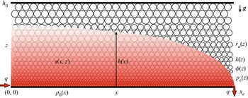
We study in this paper the quasi-steady interfacial and unsaturated flows in a horizontal porous layer with vertical heterogeneity, as sketched in figure 1. A steady state is arrived at when the drainage rate  $q$ at the edge
 $x = x_e$ equals the injection rate at the entrance
 $x = 0$. The model problem is mainly inspired to advance our understanding of flow in porous layers in three aspects:
• Porous systems are often layered in many practical situations, exhibiting vertical heterogeneity at both the pore scale and reservoir scale (e.g. Phillips Reference Phillips1991; Dullien Reference Dullien1992; Gasda & Celia Reference Gasda and Celia2005; Cowton et al. Reference Cowton, Neufeld, White, Bickle, White and Chadwick2016; Jackson et al. Reference Jackson, Agada, Reynolds and Krevor2018). Interfacial and unsaturated flows in heterogeneous porous layers adjust correspondingly and need to be characterised, including the propagation of gravity currents (e.g. Huppert & Woods Reference Huppert and Woods1995; Hinton & Woods Reference Hinton and Woods2018), edge drainage (e.g. Zheng et al. Reference Zheng, Soh, Huppert and Stone2013), converging currents (e.g. Zheng, Christov & Stone Reference Zheng, Christov and Stone2014), imbibition (e.g. Reyssat et al. Reference Reyssat, Sangne, Nierop and Stone2008b), onset of hydrodynamic instabilities (e.g. Al-Housseiny et al. Reference Al-Housseiny, Tsai and Stone2012; Grenfell-Shaw, Hinton & Woods Reference Grenfell-Shaw, Hinton and Woods2021) and dispersion of tracer particles (e.g. Hinton & Woods Reference Hinton and Woods2019). The current work focuses on upscaling unsaturated flows in quasi-steady situations.
• While asymptotic solutions have been obtained to describe the time evolution of the interface shape for gravity-current flows (e.g. Huppert & Woods Reference Huppert and Woods1995; Nordbotten & Celia Reference Nordbotten and Celia2006; MacMinn et al. Reference MacMinn, Szulczewski and Juanes2010; Gunn & Woods Reference Gunn and Woods2011; Pegler et al. Reference Pegler, Huppert and Neufeld2014; Zheng et al. Reference Zheng, Guo, Christov, Celia and Stone2015; Hinton & Woods Reference Hinton and Woods2018) and unsaturated flows (e.g. Bear Reference Bear1972; Golding et al. Reference Golding, Neufeld, Hesse and Huppert2011; Zheng & Neufeld Reference Zheng and Neufeld2019) in porous rocks in many situations (see also Zheng & Stone (Reference Zheng and Stone2022) for a recent review of detailed descriptions of the connection and difference of a series of studies), there is a lack of quantitative descriptions of the pressure signal within a reservoir, which is also an important feature of the flow and is likely more convenient to measure/monitor in the field.
• The model problem of quasi-steady flows, as sketched in figure 1, also mimics those in rock-core flooding experiments (e.g. Brooks & Corey Reference Brooks and Corey1964; Jackson et al. Reference Jackson, Agada, Reynolds and Krevor2018), which allows us to predict the effective relative permeability curves after appropriate flow upscaling on the basis of exact solutions of the saturation field and interface shape of the invading fluid within a heterogeneous porous layer. The influence of wetting and capillary effects, gravitational and injection forces, viscosity contrast and vertical heterogeneity of the porous layers can also be investigated quantitatively, providing an aspect different from that of standard literature.
Injection of a non-wetting fluid into a porous layer with vertical heterogeneity, characterised by a vertically varying average pore size  $r_a(z)$, permeability
 $k(z)$, porosity
 $\phi (z)$ and capillary entry pressure
 $p_e(z)$. A steady state is arrived at when the drainage rate
 $q$ at the edge
 $(x = x_e)$ equals the injection rate at the entrance
 $(x = 0)$ of the porous layer. The saturation field is denoted by
 $s(x,z)$, the interface shape is denoted by
 $h(x)$, where
 $s(x,z=h(x)) = 0$, and the background pressure is denoted by
 $p_0(x)$ along the bottom boundary (
 $z = 0$).

This paper is structured as follows. A theoretical model is first provided in § 2 to describe the saturation distribution and interface shape of the invading fluid within the porous layer sketched in figure 1, with a general assumption on flow dimension and vertical heterogeneity. This is followed by a detailed example calculation in § 3 to describe one-dimensional canonic flows in a Cartesian configuration. Four flow regimes are identified in §§ 3.1 and 3.2, representing unconfined sharp-interface flows, confined sharp-interface flows, unconfined unsaturated flows and confined unsaturated flows, key features of which are demonstrated through asymptotic solutions of the saturation field and interface shape. For each flow regime, we also provide the net pressure drop across the porous layer in § 3.3, with brief remarks on potential applications in § 3.4. Before we close the paper, asymptotic solutions for the effective relative permeability curve  $\bar k_{rn}(\bar s)$ of the invading fluid are also derived in § 4.1, along with remarks on the role of wetting and capillary effects, gravitational segregation, viscosity contrast and vertical heterogeneity.
2. Theoretical model
We start from descriptions of a quasi-steady unsaturated flow in homogeneous porous layers, such as flow in naturally homogeneous porous rocks or flow in packed-bead systems. We are provided with the relative permeability curves  $k_{rn}(s)$ and
 $k_{rw}(s)$ for both the invading non-wetting and displaced wetting fluids in such systems, together with the capillary pressure jump curve
 $p_c(s)$, e.g. fitted in power-law forms as a function of local saturation distribution
 $s(\boldsymbol {r}_{\|},z)$ according to
 \begin{equation} k_{rn}(s) = k_{rn0} s^{\alpha},\quad k_{rw}(s) = (1-s)^{\beta}\quad \mbox{and} \quad p_c(s) = p_e(1-s)^{{-}1/\varLambda},\end{equation}
where  $(\boldsymbol {r}_{\|},z) \equiv (x,y,z)$ denotes spatial location,
 $\alpha$,
 $\beta$ and
 $\varLambda$ are fitting parameters,
 $k_{rn0}$ is the end-point relative permeability of the invading non-wetting fluid and
 $p_e$ is the capillary entry pressure (e.g. Brooks & Corey Reference Brooks and Corey1964; Golding et al. Reference Golding, Neufeld, Hesse and Huppert2011). Based on these inputs, we are interested in characterising quasi-steady unsaturated flows in a porous layer with vertical heterogeneity, as shown in figure 1. The goal is to provide the saturation distribution
 $s(\boldsymbol {r}_{\|},z)$, outer envelope of the invading fluid
 $h(\boldsymbol {r}_{\|})$ and the net pressure drop
 ${\rm \Delta} p_0$ between the inlet and outlet of the porous layer, corresponding to a specific rate of fluid injection
 $q$. In the context of flow upscaling, we are also interested in obtaining an effective relative permeability curve
 $\bar k_{rn}$ for the invading fluid that connects the flow rate
 $q$ and net pressure drop
 ${\rm \Delta} p_0$ in the generalised Darcy's law.
A key assumption of this work is on the influence of average pore-radius distribution  $r_a(z)$ on main features of heterogeneity at the reservoir/core scale, such as the intrinsic permeability
 $k$, porosity
 $\phi$ and capillary entry pressure
 $p_e$. We denote
 $k_0$,
 $\phi _0$ and
 $\,p_{e0}$ as the (reference) intrinsic permeability, porosity and capillary entry pressure in a homogeneous porous layer with a constant average pore radius
 $r_0$, respectively. The influence of a varying pore radius then leads to modified expressions for the intrinsic permeability
 $k(z)$, porosity
 $\phi (z)$ and capillary entry pressure
 $p_e(z)$ in heterogeneous porous layers:
 \begin{equation} \frac{k(z)}{k_0} = \left[\frac{r_a(z)}{r_0}\right]^2,\quad \frac{\phi(z)}{\phi_0} = \left[\frac{r_a(z)}{r_0}\right]^{2/n}\quad \mbox{and} \quad \frac{p_e(z)}{p_{e0}} = \frac{r_0}{r_a(z)}. \end{equation}
In particular, (2.2a) is derived based on the assumption that the intrinsic permeability and average pore radius are related according to  $k \propto r_a^2$, which is consistent with the single-phase viscous channel flow or Hele-Shaw flow models that mimic flow in porous media. Equation (2.2b) is consistent with field observations that permeability and porosity are typically related in heterogeneous porous layers through
 $k \propto \phi ^{n}$, where
 $2 \le n \le 3$ (e.g. Phillips Reference Phillips1991; Dullien Reference Dullien1992; Huppert & Woods Reference Huppert and Woods1995; Zheng et al. Reference Zheng, Christov and Stone2014; Benham et al. Reference Benham, Bickle and Neufeld2021). For packed-bead systems or Hele-Shaw cells, it is also possible that
 $\phi$ remains constant when
 $k$ varies (due to variations in bead size or channel width), corresponding to
 $n \to +\infty$ in (2.2b) (e.g. Happel & Brenner Reference Happel and Brenner1983). Equation (2.2c) is derived based on the Young–Laplace equation for capillary pressure jump
 $p_e(z) \equiv \gamma \cos \theta /r_a(z)$, with
 $1/r_a(z)$ as an estimate for the local curvature,
 $\gamma$ denoting the interfacial tension,
 $\theta$ denoting the local contact angle and both
 $\gamma$ and
 $\theta$ are assumed not to exhibit any spatial variations in the current work. Strictly, the total curvature
 $1/r_a$ is estimated for a flat interface in a Hele-Shaw cell with gap thickness
 $2r_a$. For a capillary tube of radius
 $r_a$, it adjusts accordingly to
 $2/r_a$. As a result, the capillary pressure jump
 $p_c$ now also explicitly depends on the vertical location
 $z$ according to
 \begin{equation} p_c(s,z) = p_e(z)(1-s)^{{-}1/\varLambda}, \end{equation}
with  $p_e(z)$ given by (2.2c).
2.1. Derivation of governing equations
We assume that the interfacial and unsaturated flow in a porous layer of length  $x_e$ and thickness
 $h_0$ with
 $h_0/x_e \ll 1$ is mainly one-dimensional, as sketched in figure 1, such that gravitational–capillary equilibrium develops in the vertical direction (e.g. Golding et al. Reference Golding, Neufeld, Hesse and Huppert2011; Golding, Huppert & Neufeld Reference Golding, Huppert and Neufeld2017; Zheng & Neufeld Reference Zheng and Neufeld2019). The pressure distribution within the invading and displaced fluids
 $p_n(\boldsymbol {r}_{\|}, z)$ and
 $p_w(\boldsymbol {r}_{\|}, z)$ is then given by
 \begin{equation} \frac{\partial p_n}{\partial z} ={-}\rho_n g, \quad \frac{\partial p_w}{\partial z} ={-}\rho_w g, \end{equation}
where  $\rho _n$ and
 $\rho _w$ denote the density of the fluids and
 $g$ is gravitational acceleration. Equation (2.4a,b) immediately leads to
 \begin{equation} \frac{\partial p_c}{\partial z} ={-}{\rm \Delta} \rho g,\end{equation}
with  ${\rm \Delta} \rho \equiv \rho _n-\rho _w > 0$, by assumption, and the capillary pressure jump
 $p_c$ is given by
 \begin{equation} p_c(s,z) \equiv p_n(\boldsymbol{r}_{\|},z) - p_w(\boldsymbol{r}_{\|},z), \end{equation}
by definition. Notice that  $p_c(s=0,z) = p_e(z)$ at the fluid–fluid interface
 $z=h(\boldsymbol {r}_{\|})$, i.e. the outer envelope of the invading non-wetting fluid, where
 $s(\boldsymbol {r}_{\|},z)=h(\boldsymbol {r}_{\|}) = 0$, by definition. Then, we are able to integrate (2.5) once in the
 $z$ direction to provide
 \begin{equation} p_c(s,z) - p_e(z)={-}{\rm \Delta} \rho g [z-h(\boldsymbol{r}_{\|})],\end{equation}
and with  $p_c(s,z) = p_e(z)(1-s)^{-1/\varLambda }$, we obtain the saturation distribution
 \begin{equation} s(\boldsymbol{r}_{\|},z) = 1-\left(1-\frac{{\rm \Delta} \rho g [z-h(\boldsymbol{r}_{\|})]}{p_e(z)}\right)^{-\varLambda}. \end{equation}
Recall that the capillary entry pressure  $p_e(z) \equiv \gamma \cos \theta /r_a(z)$. The task is then to find
 $h(\boldsymbol {r}_{\|})$, the interface shape.
To do this, we start by calculating the pressure distribution within both fluids. We denote  $p_0(\boldsymbol {r}_{\|})$ as the pressure distribution within the invading fluid along the bottom substrate. Then, by integrating (2.4a,b) from
 $z=0$ upwards, we obtain
 $$\begin{gather} p_n(\boldsymbol{r}_{\|},z) = p_0(\boldsymbol{r}_{\|}) - \rho_n g z,\quad \mbox{for}\ 0 \le z \le h(\boldsymbol{r}_{\|}), \end{gather}$$
 $$\begin{gather}p_w(\boldsymbol{r}_{\|},z) = p_0(\boldsymbol{r}_{\|}) - \rho_n g h - p_e(z) - \rho_w(z-h), \quad \mbox{for}\ 0 \le z \le h_0, \end{gather}$$
where we have also employed the condition for capillary pressure jump  $p_n (\boldsymbol {r}_{\|},h) - p_w(\boldsymbol {r}_{\|},h) = p_e(z)$ to obtain (2.9b). It is the pressure gradient that drives the flow, which can be shown to be independent of
 $z$ as
 $$\begin{gather} \nabla_{\|}p_n(\boldsymbol{r}_{\|}) = \nabla_{\|} p_0(\boldsymbol{r}_{\|}),\quad \mbox{for}\ 0 \le z \le h(\boldsymbol{r}_{\|}), \end{gather}$$
 $$\begin{gather}\nabla_{\|} p_w(\boldsymbol{r}_{\|}) = \nabla_{\|} p_0(\boldsymbol{r}_{\|}) - {\rm \Delta} \rho g \nabla_{\|} h, \quad \mbox{for}\ 0 \le z \le h_0. \end{gather}$$
To calculate the velocity field, we next employ the generalised Darcy's law for both the invading and displaced fluids:
 $$\begin{gather} \langle \boldsymbol{u}_n \rangle (\boldsymbol{r}_{\|},z) ={-}\frac{k(z)k_{rn}(s)}{\mu_n} \nabla_{\|}p_n(\boldsymbol{r}_{\|},z), \end{gather}$$
 $$\begin{gather}\langle \boldsymbol{u}_w\rangle (\boldsymbol{r}_{\|},z) ={-}\frac{k(z)k_{rw}(s)}{\mu_w} \nabla_{\|}p_w(\boldsymbol{r}_{\|},z). \end{gather}$$
The Darcy velocities  $\langle \boldsymbol {u}_n \rangle$ and
 $\langle \boldsymbol {u}_w \rangle$ are also related through a flux condition,
 \begin{equation} \boldsymbol{q} = \int_0^{h(\boldsymbol{r}_{\|})} \langle \boldsymbol{u}_n \rangle \, {\rm d}z + \int_0^{h_0} \langle \boldsymbol{u}_w \rangle \, {\rm d}z, \end{equation}
based on local continuity at steady state. By substituting (2.11a,b) into (2.12), we immediately obtain an expression for the background pressure gradient:
 \begin{equation} \nabla_{\|}p_0(\boldsymbol{r}_{\|}) = \frac{- \mu_w}{NI_n(h)+I_w(h)}\boldsymbol{q} + \frac{{\rm \Delta} \rho g I_w(h)}{NI_n(h)+I_w(h)}\nabla_{\|}h(\boldsymbol{r}_{\|}),\end{equation}
where  $N \equiv \mu _w/\mu _n$ is the viscosity ratio and
 ${\rm \Delta} \rho \equiv \rho _n-\rho _w > 0$ is the density difference. Meanwhile, the integrals
 $I_n(h)$ and
 $I_w(h)$ in (2.13) are defined as
 \begin{equation} I_n(h) \equiv \int_0^{h(\boldsymbol{r}_{\|})}k(z)k_{rn}(s)\,{\rm d}z\quad \mbox{and}\quad I_w(h) \equiv \int_0^{h_0}k(z)k_{rw}(s)\,{\rm d}z, \end{equation}
which characterise the overall influence of permeability distribution across the entire thickness  $h_0$ of the porous layers on the flow of the invading and displaced fluids, respectively. Equation (2.13) can also be integrated once along the
 $\boldsymbol {r}_{\|}$ direction to provide the pressure drop due to viscous resistance.
In addition, the local continuity equation for steady incompressible flow of the invading and displaced fluids can be written as
 $$\begin{gather} \nabla_{\|} \boldsymbol{\cdot} \int_0^{h(\boldsymbol{r}_{\|})}\langle \boldsymbol{u}_n \rangle (\boldsymbol{r}_{\|},z)\,{\rm d}z = 0, \end{gather}$$
 $$\begin{gather}\nabla_{\|} \boldsymbol{\cdot} \int_0^{h_0}\langle \boldsymbol{u}_w \rangle (\boldsymbol{r}_{\|},z)\,{\rm d}z = 0. \end{gather}$$
By substituting (2.13) and (2.11a) into (2.15a), we obtain a differential equation for the interface shape  $h(\boldsymbol {r}_{\|})$ as
 \begin{equation} \nabla_{\|}\boldsymbol{\cdot} \left[\frac{N I_n(h)}{N I_n(h) + I_w(h)}\boldsymbol{q}\right] - \frac{{\rm \Delta} \rho g}{\mu_n} \nabla_{\|} \boldsymbol{\cdot} \left[\frac{I_n(h) I_w(h)}{N I_n(h) + I_w(h)} \nabla_{\|} h \right] = 0. \end{equation}
Physically, (2.16) indicates that the shape of the fluid–fluid interface  $h(\boldsymbol {r}_{\|})$ is determined based on the competition between gravitational and injection forces, while it is also impacted by the viscosity contrast
 $N$, permeability variations and wetting and capillary forces through (2.14a,b).
Providing appropriate boundary conditions, the interface shape  $h(\boldsymbol {r}_{\|})$ can then be calculated by solving (2.16). Typical boundary conditions for the interface shape
 $h(\boldsymbol {r}_{\|})$ can be provided at the inlet
 $\boldsymbol {r}_{\|} = \boldsymbol {0}$ and outlet
 $\boldsymbol {r}_{\|} = \boldsymbol {r}_{||e}$ as
 $$\begin{gather} \left[\frac{N I_n(h)}{N I_n(h) + I_w(h)}\boldsymbol{q} - \frac{{\rm \Delta} \rho g}{\mu_n} \frac{I_n(h) I_w(h)}{N I_n(h) + I_w(h)} \nabla_{\|} h \right]\bigg|_{\boldsymbol{r}_{\|}=\boldsymbol{0}} = \boldsymbol{q}, \end{gather}$$
 $$\begin{gather}h(\boldsymbol{r}_{||e}) = 0. \end{gather}$$
In fact, it is convenient first to integrate (2.16) once, and with the flux condition (2.17a), we obtain
 \begin{equation} I_n(h) \nabla_{\|} h ={-}\frac{\mu_n}{{\rm \Delta} \rho g}\boldsymbol{q} \end{equation}
for the profile shape  $h(\boldsymbol {r}_{\|})$, which is ready to be solved with the zero-thickness (Dirichlet) condition (2.17b) at the edge.
Once the interface shape  $h(\boldsymbol {r}_{\|})$ is known, the saturation distribution
 $s(\boldsymbol {r}_{\|},z)$ can be obtained based on (2.8), and the pressure drop
 ${\rm \Delta} p_0$ can also be obtained by integrating (2.13) along
 $\boldsymbol {r}_{\|}$ between the inlet and outlet of the porous layer. In principle, the analysis above applies for any vertical distribution of the average pore size
 $r_a(z)$ and any functional form of the relative permeability curves
 $k_{rn}(s)$ and
 $k_{rw}(s)$ and the capillary pressure jump curve
 $p_c(s)$. It is also of interest to note that, at any quasi-steady state, the interface shape
 $h(\boldsymbol {r}_{\|})$, saturation distribution
 $s(\boldsymbol {r}_{\|},z)$ and net pressure drop
 ${\rm \Delta} p_0$ are all independent of the vertical variation of porosity.
3. Example calculations
We next look into one-dimensional canonic flows in a Cartesian configuration when  $\boldsymbol {r}_{\|}=x\,\boldsymbol {e}_x$ and
 $\boldsymbol {q}=q\,\boldsymbol {e}_x$, as shown in figure 1. To demonstrate the major ideas, we assume that the relative permeability and capillary pressure jump curves all follow power-law forms (2.1a–c). Meanwhile, for simplicity and without loss of generality, we assume that the average pore radius also follows a power-law distribution in the vertical direction:
 \begin{equation} r_a = r_0 z^{\delta},\end{equation}
where  $\delta \ge 0$ describes the nonlinearity in pore size distribution and
 $r_a=r_0$ for homogeneous porous layers (with
 $\delta =0$). Substituting (3.1) into (2.2a–c) provides that
 $k(z) = k_0z^{2\delta }$,
 $\phi (z) \propto z^{2\delta /n}$ and
 $p_e(z) \propto z^{-\delta }$. Correspondingly,
 $\delta = 1/2$ indicates a linear variation in intrinsic permeability, while
 $\delta = 1$ indicates a linear variation in average pore radius. Imposing power-law forms of heterogeneity in example calculations is consistent with a series of earlier studies on gravity-current flows (e.g. Huppert & Woods Reference Huppert and Woods1995; Hinton & Woods Reference Hinton and Woods2018, imbibition (e.g. Reyssat et al. Reference Reyssat, Courbin, Reyssat and Stone2008a,Reference Reyssat, Sangne, Nierop and Stoneb, onset of hydrodynamic instability (e.g. Al-Housseiny et al. Reference Al-Housseiny, Tsai and Stone2012; Grenfell-Shaw et al. Reference Grenfell-Shaw, Hinton and Woods2021, gravity-driven drainage (e.g. Zheng et al. Reference Zheng, Soh, Huppert and Stone2013, converging gravity currents (e.g. Zheng et al. Reference Zheng, Christov and Stone2014; Zheng, Ghodgaonkar & Christov Reference Zheng, Ghodgaonkar and Christov2021 and tracer dispersion (e.g. Hinton & Woods Reference Hinton and Woods2019 in porous media, Hele-Shaw cells and microchannels.
3.1. Governing equation and non-dimensionalisation
The saturation distribution (2.8) and permeability integrals (2.14a,b) in this case become
 $$\begin{gather} s(x,z) = 1-\left(1-\frac{{\rm \Delta} \rho g r_0 z^{\delta} [z-h(x)]}{\gamma\, \cos \,\theta}\right)^{-\varLambda}, \end{gather}$$
 $$\begin{gather}I_n(h) \equiv \int_0^{h(x)}k_0k_{rn0} z^{2\delta}s^{\alpha}\,{\rm d}z\quad \mbox{and}\quad I_w(h) \equiv \int_0^{h_0}k_0 z^{2\delta} (1-s)^{\beta}\,{\rm d}z, \end{gather}$$
while the interface shape  $h(x)$ and background pressure gradient
 ${\rm d}p_0/{\rm d}\kern0.7pt x$ become
 \begin{equation} \frac{{\rm d}}{{\rm d}\kern0.7pt x} \left[\frac{q N I_n(h)}{N I_n(h) + I_w(h)}\right] - \frac{{\rm \Delta} \rho g}{\mu_n} \frac{{\rm d}}{{\rm d}\kern0.7pt x} \left[\frac{I_n(h) I_w(h)}{N I_n(h) + I_w(h)} \frac{{\rm d}h}{{\rm d}\kern0.7pt x} \right] = 0 \end{equation}
and
 \begin{equation} \frac{{\rm d}p_0}{{\rm d}\kern0.7pt x} ={-}\frac{q \mu_w}{NI_n(h)+I_w(h)} + \frac{{\rm \Delta} \rho g I_w(h)}{NI_n(h)+I_w(h)}\frac{{\rm d} h}{{\rm d}\kern0.7pt x},\end{equation}
respectively.
Appropriate boundary conditions can be provided for (3.3) at the inlet  $x=0$ and outlet
 $x=x_e$ of a porous layer as
 $$\begin{gather} \left.\left[\frac{q N I_n(h)}{N I_n(h) + I_w(h)} - \frac{{\rm \Delta} \rho g}{\mu_n} \frac{I_n(h) I_w(h)}{N I_n(h) + I_w(h)} \frac{{\rm d}h}{{\rm d}\kern0.7pt x}\right]\right|_{x=0} = q, \end{gather}$$
 $$\begin{gather}h(x_e) = 0, \end{gather}$$
and the interface shape  $h(x)$ can then be obtained by solving (3.3) with (3.5). In particular, with (3.5a), (3.3) can be integrated once to provide
 \begin{equation} I_n(h) \frac{{\rm d}h}{{\rm d}\kern0.7pt x} ={-}\frac{\mu_n q}{{\rm \Delta} \rho g}, \end{equation}
which is to be solved subject to boundary condition (3.5b) at the outlet/edge. It is of interest to note again that (3.3) to (3.6) apply for any form of  $k_{rn}(s)$,
 $k_{rw}(s)$ and
 $p_c(s)$, besides the power-law form (2.1a–c) we have employed here in the example calculations.
We next non-dimensionalise (3.6) and (3.5b) by defining dimensionless shape  $\bar h(\bar x) \equiv h/h_0$, length
 $\bar x \equiv x/x_e$, height
 $\bar z \equiv z/h_0$ and permeability integral
 $\bar I_n \equiv I_n/k_0k_{rn0} h_0^{2\delta +1}$, which then leads to
 $$\begin{gather} \bar I_n(\bar h) \frac{{\rm d}\bar h}{{\rm d}\kern0.7pt \bar x} ={-} \varGamma\quad \mbox{and}\quad \bar I_n(\bar h) = \int_0^{\bar h(\bar x)} \bar z^{2\delta} s^{\alpha}\,{\rm d}\bar z, \end{gather}$$
 $$\begin{gather}\mbox{s.t.}\ \bar h(1) = 0, \end{gather}$$
where  $\varGamma \equiv \mu _n q x_e/ {\rm \Delta} \rho g k_0k_{rn0} h_0^{2\delta +2}$ is defined to characterise the competition between the injection and gravitational forces. Physically,
 $\varGamma$ also represents a rescaled injection rate
 $q$ or velocity
 $q/h_0$ for the non-wetting injecting fluid.
The saturation distribution (3.2a) and pressure gradient (3.4), in addition, can be rearranged to provide
 $$\begin{gather} s(\bar x, \bar z) = 1-(1-B \bar z^{\delta} [\bar z- \bar h(\bar x)])^{-\varLambda}, \end{gather}$$
 $$\begin{gather}\frac{{\rm d}\bar p_0}{{\rm d} \bar x} ={-}\frac{\bar N}{\bar N \bar I_n(\bar h)+ \bar I_w(\bar h)} + \frac{\varGamma^{{-}1} \bar I_w(\bar h)}{\bar N \bar I_n(\bar h)+ \bar I_w(\bar h)}\frac{{\rm d} \bar h}{{\rm d}\kern0.7pt \bar x}, \end{gather}$$
where  $s \in [0,1]$ for
 $\bar z \in [0, \bar h]$ and
 $\bar N \equiv Nk_{rn0}$ is a modified viscosity ratio, and the dimensionless background pressure
 $\bar p_0(\bar x) \equiv p_0(x)/p_{0c}$ is rescaled based on
 $\,p_{0c} = \mu _n q x_e/k_0 k_{rn0} h_0^{2\delta +1}$, a characteristic injection pressure. A Bond number also appears in the saturation distribution (3.8a), defined as
 $B \equiv {\rm \Delta} \rho g r_0 h_0^{\delta +1}/\gamma \cos \theta$ to characterise the competition between the gravitational and capillary forces. Bond number
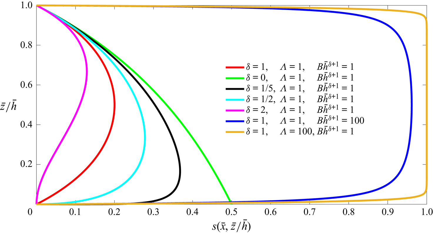
 $B$ can also be understood as a rescaled buoyancy force. Solution (3.8a) for the saturation distribution is shown in figure 2 for different parameter values of
 $\delta$,
 $\varLambda$ and
 $B\bar h^{\delta +1}$. It is shown that for the specific power-law form of vertical heterogeneity (
 $r_a(z) = r_0 z^{\delta }$), the saturation distribution is non-monotonic, as it is difficult for the invading fluid to displace the ambient fluid in a thin layer close to the bottom boundary
 $z=0$. It is also shown that, as
 $\varLambda \to +\infty$ or
 $B\bar h^{\delta +1} \to +\infty$, the invading fluid completely replaces the displaced fluid in the porous layer, i.e.
 $s(\bar x, \bar z) \to 1^-$ for
 $\bar z \in [0,\bar h(\bar x)]$, at any location
 $\bar x$.
Saturation distribution  $s(\bar x, \bar z)$ of the invading fluid along the vertical direction
 $\bar z$ at any horizontal location
 $\bar x \in [0,1]$ according to (3.8a). The solutions are impacted by three dimensionless parameters
 $\delta$,
 $\varLambda$ and
 $B\bar h^{\delta +1}$, and the solution of
 $s(\bar x, \bar z)$ approaches the sharp-interface description (3.11) as
 $\varLambda \to +\infty$ or
 $B\bar h^{\delta +1} \to +\infty$.

Meanwhile, the vertical integral  $I_w$ is rescaled according to
 $\bar I_w(\bar h) \equiv I_w/k_0 h_0^{2\delta +1}$, such that
 \begin{equation} \bar I_w(\bar h) \equiv \int_0^{1}\bar z^{2\delta} (1-s)^{\beta}\,{\rm d}\bar z.\end{equation}
The dimensionless net pressure drop  ${\rm \Delta} \bar p_0$ throughout a porous layer can also be calculated as
 \begin{equation} {\rm \Delta} \bar p_0 = \int_0^1\left[-\frac{\bar N}{\bar N \bar I_n(\bar h)+ \bar I_w(\bar h)} + \frac{\varGamma^{{-}1} \bar I_w(\bar h)}{\bar N \bar I_n(\bar h)+ \bar I_w(\bar h)}\frac{{\rm d} \bar h}{{\rm d}\kern0.7pt \bar x}\right]\, {\rm d}\kern0.7pt \bar x,\end{equation}
also rescaled by  $\,p_{0c}$.
We are now ready to solve (3.7) for the interface shape  $\bar h(\bar x)$, which is impacted by five dimensionless parameters: the distribution parameter for the average pore size (
 $\delta$), the exponent of the relative permeability curve of the injecting fluid (
 $\alpha$), the exponent of the capillary pressure jump curve that indicates the pore size distribution (
 $\varLambda$), the ratio of injection over gravitational forces (
 $\varGamma$) and a Bond number that describes the competition between the gravitational and capillary forces (
 $B$). Based on (3.8), it is also suggested that the saturation distribution
 $s(\bar x, \bar z)$ is impacted by five dimensionless parameters
 $\delta$,
 $\alpha$,
 $\varLambda$,
 $\varGamma$ and
 $B$. Finally, besides
 $\delta$,
 $\alpha$,
 $\varLambda$,
 $\varGamma$ and
 $B$, the pressure drop
 ${\rm \Delta} \bar p_0$ is further impacted by
 $\beta$, the exponent in the relative permeability curve for the displaced fluid, and
 $\bar N$, a modified viscosity ratio between the injecting and displaced fluids. The definition and physical meaning of the eight dimensionless parameters are summarised in table 1.
Definition and physical meaning of eight dimensionless parameters  $\delta$,
 $\alpha$,
 $k_{rn0}$,
 $\beta$,
 $\varLambda$,
 $\bar N$,
 $B$ and
 $\varGamma$ for one-dimensional canonic flows in heterogeneous porous layers.

We then move on to discuss several important/comprehensive asymptotic regimes of the flow, as described by (3.7). Specifically, knowing that the porous layer has a finite depth, depending on the (dimensionless) injection rate  $\varGamma$, unconfined and confined flow regimes become a natural and important outcome of the physical system, which is a focus of the current work. Another focus of the asymptotic analysis is to illustrate whether the injected and displaced fluids exhibit a sharp interface between each other, or whether there is a gradual change in fluid saturation. This is also an important feature of the quasi-steady flow and is characterised by the dimensionless parameter
 $B$, a measurement of the competition between capillary and gravitational forces. We next provide detailed descriptions of the flow in each regime.
3.2. Sharp-interface and unsaturated flow regimes
We next explore asymptotic behaviours of the interface shape  $\bar h(\bar x)$, saturation distribution
 $s(\bar x, \bar z)$ and net pressure drop
 ${\rm \Delta} \bar p_0$ across a porous layer. In particular, we look into the sharp-interface regime, when the flow is dominated by the viscous and gravitational forces, and also the unsaturated flow regime, when the flow is significantly impacted by the wetting and capillary effects. For simplicity and without loss of generality, we impose
 $\alpha =\beta =2$ for the relative permeability curves (2.1a,b) for flow in homogeneous porous layers, which allows us to gain more analytical insights. Brief remarks are also provided on the influence of
 $\alpha$ and
 $\beta$ in Appendix A.
3.2.1. Sharp-interface regime
When  $B \gg 1$ or
 $\varLambda \gg 1$, the influence of wetting and capillary forces becomes negligible on the saturation field, as the thickness of the capillary fringe approaches zero. In this regime, the saturation distribution (3.8) approaches
 \begin{equation} s(\bar x, \bar z) = \left\{\begin{array}{ll} 1, & 0 \le \bar z \le \bar h(\bar x), \\ 0, & \bar h(\bar x) < \bar z \le 1, \end{array} \right.\end{equation}
which indicates a sudden change of fluid saturation across a sharp interface  $\bar h (\bar x)$ between the injecting and displaced fluids. The permeability integrals
 $\bar I_n(\bar h)$ and
 $\bar I_w(\bar h)$ reduce to
 \begin{equation} \bar I_n(\bar h) = \frac{\bar h^{2\delta+1}}{2\delta + 1}\quad \mbox{and}\quad \bar I_w(\bar h) = \frac{1-\bar h^{2\delta+1}}{2\delta + 1}, \end{equation}
correspondingly. The interface shape  $\bar h(\bar x)$ is then determined by solving
 \begin{equation} \bar h^{2\delta+1} \frac{{\rm d}\bar h}{{\rm d}\kern0.7pt \bar x} ={-} (2\delta + 1)\varGamma, \end{equation}
subject to  $\bar h(1) = 0$, which leads to
 \begin{equation} \bar h(\bar x) = \left[\frac{(2\delta+1)\varGamma}{2(\delta+1)}\right]^{1/2(\delta+1)} (1-\bar x)^{1/2(\delta+1)}. \end{equation}
As indicated by (3.14),  $\bar h(\bar x)$ is under the influence of
 $\delta$ and
 $\varGamma$.
Since the porous layer has a finite thickness, solution (3.14) holds across the entire domain  $\bar x \in [0,1]$ only when
 $\bar h(0) = [(2\delta +1)\varGamma /2(\delta +1)]^{1/2(\delta +1)} \le 1$, when the flow is ‘unconfined’. Correspondingly, lower injection rates are required, such that
 $\varGamma \le 2(\delta +1)/(2\delta +1)$. In contrast, at higher injection rates with
 $\varGamma > 2(\delta +1)/(2\delta +1)$, we impose
 $\bar h(\bar x) = 1$ for
 $\bar x \in [0, 1-2(\delta +1)/(2\delta +1)\varGamma ]$, a region close to the inlet of the porous layer, while we apply (3.14) for
 $\bar x \in [1-2(\delta +1)/(2\delta +1)\varGamma, 1]$, a region near the outlet, i.e.
 \begin{equation} \bar h(\bar x) = \left\{\begin{array}{ll} 1, & 0 \le \bar x \le 1-\dfrac{2(\delta+1)}{(2\delta+1)\varGamma}, \\ \left[\dfrac{(2\delta+1)\varGamma}{2(\delta+1)}\right]^{1/2(\delta+1)} (1-\bar x)^{1/2(\delta+1)}, & 1-\dfrac{2(\delta+1)}{(2\delta+1)\varGamma} \le \bar x \le 1. \end{array} \right.\end{equation}
The fluid–fluid interface in this situation attaches at both the top and bottom boundaries of the porous layer, as the flow becomes ‘confined’.
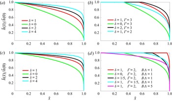
Representative interface shapes are shown in figure 3(a,b) for both the unconfined and confined flow regimes, described by (3.14) and (3.15), respectively. The solution curves in figure 3(a,b) reveal a boundary-layer structure near the edge ( $\bar x = 1$) with the most significant gravitational effects. Such a structure also corresponds to the zero-thickness boundary condition at the edge, i.e.
 $\bar h(\bar x = 1) = 0$. It is also of interest to refer to a series of unsteady buoyancy-driven edge-drainage experiments in Hele-Shaw cells, when inertial effects are negligible (see, e.g. figures 3 and 5 in Zheng et al. (Reference Zheng, Soh, Huppert and Stone2013)): the boundary-layer structure is observed in these experiments and well captured by unsteady models at intermediate times, imposing the same zero-thickness boundary condition at the edge. However, the zero-thickness boundary condition fails when the influence of inertia is non-negligible (Momen et al. Reference Momen, Zheng, Bou-Zeid and Stone2017).
Shape of the rescaled fluid–fluid interface  $\bar h(\bar x)/\bar h(0)$ in a confined porous layer: (a,b) the sharp-interface regime and (c,d) the unsaturated flow regime. The flow is unconfined in (a,c) at lower injection rates, while the flow becomes confined in (b,d) at higher injection rates, i.e.
 $\varGamma > 2(\delta +1)/(2\delta +1)$ in (b) or
 $\varGamma >8 B^2 \varLambda ^2(\delta +1)/(4\delta +1)(4\delta +2)(4\delta +3)$ in (d), when the interface attaches at both the top and bottom boundaries.

It is of interest to note that the distinct interface shapes for unconfined and confined flows seem to be related to the early-time unconfined and late-time confined self-similar interface shapes in a series of early studies on the dynamics of gravity-current flows from fluid injection into confined porous layers (e.g. Huppert & Woods Reference Huppert and Woods1995; Nordbotten & Celia Reference Nordbotten and Celia2006; MacMinn et al. Reference MacMinn, Szulczewski and Juanes2010; Gunn & Woods Reference Gunn and Woods2011; Pegler et al. Reference Pegler, Huppert and Neufeld2014; Zheng et al. Reference Zheng, Guo, Christov, Celia and Stone2015; Hinton & Woods Reference Hinton and Woods2018; Zheng & Neufeld Reference Zheng and Neufeld2019; Zheng & Stone Reference Zheng and Stone2022). However, the confined interface shapes typically depend on the viscosity contrast  $N \equiv \mu _w/\mu _n$ for unsteady flows in the aforementioned earlier studies, while no such dependence appears for steady flows considered here. This is because the
 $\bar N$-dependent terms cancel out each other for steady flows, as we arrive at (3.7a) from (3.3) for the interface shape
 $\bar h(\bar x)$. Nevertheless,
 $\bar N$ remains in solution (3.8b) for the background pressure gradient
 $\partial \bar p_0/\partial \bar x$ and in (3.10) for the net pressure drop
 ${\rm \Delta} \bar p_0$, as we discuss later in § 3.3.
3.2.2. Unsaturated flow regime
When  $B \ll 1$, at leading order, the saturation distribution (3.8) reduces to
 \begin{equation} s(\bar x, \bar z) = B \varLambda [\bar h(\bar x) - \bar z] \bar z^{\delta} + O(B^2). \end{equation}
Equation (3.16) indicates that  $s(\bar x, 0) = 0$ and
 $s[\bar x, \bar h(\bar x)] = 0$, so the saturation distribution
 $s(\bar x, \bar z)$ is no longer monotonic along any vertical line at any horizontal location
 $\bar x$. Meanwhile, the relative permeability integrals reduce to
 \begin{equation} \left.\begin{array}{c@{}} \bar I_n(\bar h) = \dfrac{2B^2 \varLambda^2 \bar h^{4\delta+3}}{(4\delta+1)(4\delta+2)(4\delta+3)} + O(B^3) \quad \mbox{and}\\ \bar I_w(\bar h) = \dfrac{1}{2\delta+1} - \dfrac{2B\varLambda \bar h^{3\delta+2}}{(3\delta+1)(3\delta+2)} + O(B^2) . \end{array}\right\} \end{equation}
The outer envelope of the invading fluid  $\bar h(\bar x)$, at leading order, is then described by
 \begin{equation} \bar h^{4\delta+3} \frac{{\rm d}\bar h}{{\rm d}\kern0.7pt \bar x} ={-} \frac{(4\delta+1)(4\delta+2)(4\delta+3)\varGamma}{2 B^2 \varLambda^2}, \end{equation}
subject to  $\bar h(1)=0$, which leads to a profile shape
 \begin{equation} \bar h(\bar x) = \left[\frac{(4\delta+1)(4\delta+2)(4\delta+3)\varGamma}{8\,(\delta+1)B^2 \varLambda^2}\right]^{{1}/{4(\delta+1)}} \left(1-\bar x\right)^{{1}/{4(\delta+1)}}, \end{equation}
under the influence of  $\delta$,
 $\varGamma$ and
 $B \varLambda$.
Again, since the porous layer has a finite thickness, solution (3.19) applies throughout the entire domain  $\bar x \in [0,1]$ only in the ‘unconfined’ regime when
 $\bar h(0) \le 1$, which corresponds to lower injection rates at
 $\varGamma \le 8 B^2 \varLambda ^2 (\delta +1)/(4\delta +1)(4\delta +2)(4\delta +3)$. On the other hand, at higher injection rates
 $\varGamma >8 B^2 \varLambda ^2(\delta +1)/(4\delta +1)(4\delta +2)(4\delta +3)$, we impose
 $\bar h(\bar x) = 1$ in a region close to the inlet of the porous layer
 $\bar x \in [0,1-8(\delta +1)B^2 \varLambda ^2/(4\delta +1)(4\delta +2)(4\delta +3)\varGamma ]$, i.e.
 \begin{align} \bar h(\bar x) =
\left\{ \small\begin{array}{ll} 1, & 0 \le \bar x \le
1-\dfrac{8(\delta+1)B^2
\varLambda^2}{(4\delta+1)(4\delta+2)(4\delta+3)\varGamma},
\\
{\begin{array}{@{}l@{}}\left[\dfrac{(4\delta+1)(4\delta+2)(4\delta+3)\varGamma}{8(\delta+1)B^2
\varLambda^2}\right]^{{1}/{4(\delta+1)}}\\ (1-\bar
x)^{{1}/{4(\delta+1)}}\end{array}}, & 1-\dfrac{8(\delta+1)B^2
\varLambda^2}{(4\delta+1)(4\delta+2)(4\delta+3)\varGamma}
\le \bar x \le 1. \end{array}
\right.\end{align}
In this case, the interface attaches at both the top and bottom boundaries of the porous layer. Solutions (3.19) and (3.20) are shown in figures 3(c) and 3(d), respectively, which illustrate both unconfined and confined flows at lower and higher injection rates.
Correspondingly, at lower injection rates  $\varGamma \le 8 B^2 \varLambda ^2(\delta +1)/(4\delta +1)(4\delta +2)(4\delta +3)$, a leading-order approximation for the saturation distribution
 $s(\bar x, \bar z)$ is available by substituting (3.19) back into (3.16) as
 \begin{equation} s(\bar x, \bar z) = B \varLambda \left(\left[\dfrac{(4\delta+1)(4\delta+2)(4\delta+3) \varGamma}{8(\delta+1)B^2 \varLambda^2}\right]^{{1}/{4(\delta+1)}} (1-\bar x)^{{1}/{4(\delta+1)}} - \bar z\right) \bar z^{\delta},\end{equation}
which is also impacted by  $\delta$,
 $\varGamma$ and
 $B \varLambda$. At higher injection rates
 $\varGamma > 8B^2 \varLambda ^2(\delta +1)/(4\delta +1)(4\delta +2)(4\delta +3)$, the outer envelope of the invading fluid attaches to both the top and bottom boundaries, and we hence substitute (3.20) back into (3.16) to provide
 \begin{align} s(\bar x, \bar z) = \left\{ \small\begin{array}{ll} B \varLambda (1 - \bar z) \bar z^{\delta}, & 0 \le \bar x \le 1-\dfrac{8(\delta+1)B^2 \varLambda^2}{(4\delta+1)(4\delta+2)(4\delta+3)\varGamma}, \\ \begin{aligned} & B\varLambda \left(\left[\dfrac{(4\delta+1)(4\delta+2)(4\delta+3) \varGamma}{8(\delta+1)B^2 \varLambda^2}\right]^{{1}/{4(\delta+1)}} \right.\\ & \quad \left. \vphantom{\dfrac{8(\delta+1)B^2 \varLambda^2}{(4\delta+1)(4\delta+2)(4\delta+3)\varGamma}}(1-\bar x)^{{1}/{4(\delta+1)}} - \bar z\right) \bar z^{\delta}, \end{aligned} & 1-\dfrac{8(\delta+1)B^2 \varLambda^2}{(4\delta+1)(4\delta+2)(4\delta+3)\varGamma} \le \bar x \le 1, \end{array} \right.\end{align}
as a leading-order approximation for the saturation distribution in the ‘confined’ regime. Solution (3.22) also indicates that, in a region close to the inlet of a porous layer  $\bar x \in [0,1-8(\delta +1)B^2 \varLambda ^2/(4\delta +1)(4\delta +2)(4\delta +3)\varGamma ]$, the saturation does not exhibit dependence on
 $\bar x$ and only varies vertically with
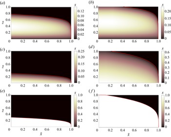
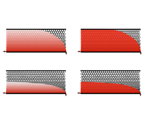
 $\bar z$. The saturation distributions (3.21) and (3.22), with representative parameter values, are demonstrated in figure 4(a–d) for unsaturated flows in both heterogeneous and homogeneous porous layers and for both unconfined and confined flows. Solution (3.11) in the sharp-interface regime (
 $B \gg 1$) is also shown in figure 4(e,f) as a comparison.
Saturation distribution of the invading fluid in the unsaturated flow regime according to (3.21) and (3.22): (a,b) unsaturated flows in heterogeneous porous layers ( $\delta =1$) and (c,d) in homogeneous porous layers (
 $\delta =0$). As a comparison, the sudden change in saturation in the sharp-interface regime is also shown in (e,f) according to (3.11). The location of the interface
 $\bar z = \bar h (\bar x)$ is marked as the red curves in (a–f), where the saturation
 $s(\bar x, \bar z)$ drops to zero. Parameter values: (a)
 $\delta =1, \varGamma = 1/100, B \varLambda =1$, (b)
 $\delta =1, \varGamma = 1/10, B \varLambda =1$, (c)
 $\delta =0, \varGamma = 1/100, B \varLambda =1$, (d)
 $\delta =0, \varGamma = 3/2, B \varLambda =1$, (e)
 $\delta =1, \varGamma = 1/100$ and (f)
 $\delta =1, \varGamma = 3/2$.

3.3. Background pressure drop along porous layers
We next calculate the net drop of the background pressure  $p_0(x)$ between the inlet and outlet of the porous layer under different injection rate
 $q$. It is often more convenient to measure/monitor the pressure signals in many practical situations, compared with the interface shape
 $h(x)$ and/or the saturation distribution
 $s(x,z)$. The pressure drop also provides information on how much work is needed for fluid injection to occur at rate
 $q$. It is standard to present the dimensionless results of
 ${\rm \Delta} \bar p_0$ as a function of
 $\varGamma$, a dimensionless flow rate, based on (3.10). It is of interest to note that
 $1/\varGamma$ can also be seen as an effective Reynolds number, so the
 ${\rm \Delta} \bar p_0$ versus
 $\varGamma$ chart also connects with the standard literature for pressure loss due to viscous resistance in other contexts such as flow in open channels and in pipes.
Within the sharp-interface regime ( $B \gg 1$ or
 $\varLambda \gg 1$), by substituting (3.12a,b) into (3.10), we obtain
 \begin{equation} {\rm \Delta} \bar p_0 = \int_0^1\,\left[-\frac{(2\delta + 1)\bar N }{1 + (\bar N-1) \bar h^{2\delta+1}} + \frac{\varGamma^{{-}1} (1-\bar h^{2\delta+1})}{1 + (\bar N-1) \bar h^{2\delta+1}}\frac{{\rm d} \bar h}{{\rm d}\kern0.7pt \bar x}\right]\, {\rm d}\kern0.7pt \bar x. \end{equation}
Since  $\bar h(\bar x)$ is already provided by (3.14) in the unconfined regime at lower injection rates (
 $\varGamma \le 2(\delta +1)/(2\delta +1)$) or (3.15) in the confined regime at higher injection rates (
 $\varGamma > 2(\delta +1)/(2\delta +1)$), the pressure drop
 ${\rm \Delta} \bar p_0$ is ready to be calculated based on (3.23). It is also shown by (3.23) that the pressure drop
 ${\rm \Delta} \bar p_0$ is impacted by the competition between the injection and gravitational forces (
 $\varGamma$), modified viscosity ratio (
 $\bar N$) and vertical heterogeneity of the porous layer (
 $\delta$).
Furthermore, at ultralow injection rates ( $\varGamma \ll 1$), the thickness of the invading fluid becomes much smaller than the thickness of the porous layer (i.e.
 $\bar h \ll 1$). Solution (3.23) in this regime can be further rearranged to provide an explicit expression,
 \begin{equation} {\rm \Delta} \bar p_0 \sim{-} (2\delta + 1)\bar N - \varGamma^{-({2\delta+1})/{2(\delta+1)}} \left[\frac{(2\delta+1)}{2(\delta+1)}\right]^{1/{2(\delta+1)}} , \end{equation}
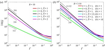
for the net drop of the background pressure  ${\rm \Delta} \bar p_0$. Solution (3.24) is plotted in figure 5(a) as a series of
 ${\rm \Delta} \bar p_0(\varGamma )$ curves, impacted by the vertical heterogeneity (
 $\delta$) and modified viscosity contrast (
 $\bar N$). In particular, it is demonstrated that the pressure drop exhibits power-law dependence
 ${\rm \Delta} \bar p_0 \propto \varGamma ^{-(2\delta +1)/2(\delta +1)}$ on the injection rate
 $\varGamma$ at sufficiently low injection rates. This is due to the nonlinear dependence of the interface shape on the injection rate, as well as the additional contribution of gravitational-driven flow.
Background pressure drop  ${\rm \Delta} \bar p_0$ along a porous layer versus the rescaled injection rate
 $\varGamma$: (a) solution (3.24) in the sharp-interface regime (e.g.
 $B \gg 1$) and (b) solution (3.26) in the unsaturated flow regime (
 $B \ll 1$). The slopes of
 $\varGamma ^{-(2\delta +1)/2(\delta +1)}$ and
 $\varGamma ^{-(4\delta +1)/4(\delta +1)}$ are also shown, and the impacts of
 $\delta$,
 $\bar N$ and
 $B\varLambda$ are demonstrated. Notice that solutions (3.24) and (3.26) only apply at lower injection rates
 $\varGamma \ll \min \{1,B\varLambda \}$.

Within the unsaturated flow regime ( $B \ll 1$), similarly, we can substitute (3.17a,b) into (3.10) and obtain the background pressure drop:
 \begin{equation} {\rm \Delta} \bar p_0 = \int_0^1\left(\dfrac{-\bar N + \varGamma^{{-}1} \left[\frac{1}{2\delta+1} - \frac{2B\varLambda \bar h^{3\delta+2}}{(3\delta+1)(3\delta+2)}\right] \frac{{\rm d}\bar h}{{\rm d}\kern0.7pt \bar x}}{\displaystyle \frac{1}{2\delta+1} - \frac{2B\varLambda \bar h^{3\delta+2}}{(3\delta+1)(3\delta+2)} + \frac{2B^2\varLambda^2 \bar N \bar h^{4\delta+3}}{(4\delta+1)(4\delta+2)(4\delta+3)} }\right)\, {\rm d}\kern0.7pt \bar x,\end{equation}
now with  $\bar h(\bar x)$ provided by (3.19) in the unconfined regime at lower injection rates (
 $\varGamma \le 8 B^2 \varLambda ^2(\delta +1)/(4\delta +1)(4\delta +2)(4\delta +3)$) and (3.20) in the confined regime at higher injection rates (
 $\varGamma > 8 B^2 \varLambda ^2(\delta +1)/(4\delta +1)(4\delta +2)(4\delta +3)$). Besides
 $\varGamma$,
 $\bar N$ and
 $\delta$, the net drop of background pressure
 ${\rm \Delta} \bar p_0$ is impacted by an additional parameter
 $B\varLambda$, which describes the influence of wetting and capillary forces over the gravitational force.
In addition, at ultralow injection rates ( $\varGamma \ll B^2\varLambda ^2$), all of the invading fluid accumulates within a narrow layer attaching at the bottom boundary (
 $\bar h \ll 1$). Equation (3.25) then reduces to an explicit expression,
 \begin{equation} {\rm \Delta} \bar p_0 \sim{-} (2\delta + 1)\bar N - \varGamma^{-({4\delta+3})/{4(\delta+1)}} \left[\frac{(4\delta+1)(4\delta+2)(4\delta+3)}{8(\delta+1)B^2 \varLambda^2}\right]^{{1}/{4(\delta+1)}}, \end{equation}
for the net drop of background pressure. Solution (3.26) is also plotted in figure 5(b) as the  ${\rm \Delta} \bar p_0(\varGamma )$ curves, which are also impacted by dimensionless parameters
 $\delta$,
 $\bar N$ and
 $B\varLambda$. Again, a nonlinear power-law dependence on injection rates
 ${\rm \Delta} \bar p_0 \propto \varGamma ^{-(4\delta +3)/4(\delta +1)}$ appears based on (3.26) at sufficiently low injection rates.
3.4. Implications
The analyses and calculations in § 3.3 provided quantitative descriptions of the relationship between flow rate  $q$ and pressure drop
 ${\rm \Delta} p_0$, which was not covered in earlier studies of flow in porous media (e.g. Huppert & Woods Reference Huppert and Woods1995; Nordbotten & Celia Reference Nordbotten and Celia2006; Golding et al. Reference Golding, Neufeld, Hesse and Huppert2011; Pegler et al. Reference Pegler, Huppert and Neufeld2014; Zheng et al. Reference Zheng, Guo, Christov, Celia and Stone2015). In the context of oil recovery, given an imposed pressure drop
 ${\rm \Delta} p_0$, one is ready to make estimates on the rate of outflow
 $q$ from production wells when breakthrough occurs. Similarly, one is also ready to make estimates on the rate of CO
 $_2$ leakage from geological faults during CO
 $_2$ injection at sequestration sites. Finally, one can further justify the influence of viscosity contrasts, injection and buoyancy forces, wetting and capillary forces and heterogeneity of the porous layers in the aforementioned applications.
Specifically, in the aforementioned practical contexts, providing geophysical descriptions of a heterogeneous porous layer ( $\delta$,
 $r_0$,
 $k_0$,
 $\varLambda$,
 $h_0$,
 $x_e$), viscosity and density of the invading and displaced fluids (
 $\mu _n$,
 $\mu _w$,
 $\rho _n$,
 $\rho _w$), interfacial tension and apparent contact angle (
 $\gamma$,
 $\theta$), end-point relative permeability of the invading fluid (
 $k_{rn0}$) and a target injection rate (
 $q$), one can calculate the dimensionless injection rate
 $\varGamma \equiv \mu _n q x_e/ {\rm \Delta} \rho g k_0k_{rn0} h_0^{2\delta +2}$, modified viscosity ratio
 $\bar N \equiv k_{rn0}\mu _w/\mu _n$, rescaled buoyancy force
 $B \equiv {\rm \Delta} \rho g r_0 h_0^{\delta +1}/\gamma \cos \theta$ and characteristic pressure
 $\,p_{0c} = \mu _n q x_e/k_0 k_{rn0} h_0^{2\delta +1}$. Then, based on the asymptotic solutions obtained in § 3.3 or figure 5, one is ready to obtain the dimensionless pressure drop
 ${\rm \Delta} \bar p_0$ in corresponding flow situations, and hence the net pressure drop according to
 ${\rm \Delta} p_0 = \,p_{0c} {\rm \Delta} \bar p_0$. It is then known how much pressure
 ${\rm \Delta} p_0$ is needed to sustain a target rate
 $q$ of fluid injection in oil production. Alternatively, a leakage rate
 $q$ can be informed for a given pressure difference
 ${\rm \Delta} p_0$ between the inlet and outlet of a porous layer (e.g. through measurements in the field).
4. Discussions and summary
4.1. Remarks on flow upscaling and effective relative permeability curves
The model problem we studied here is also related to rock-core flooding experiments, typically employed to provide the effective relative permeability curves for practical use, e.g. in petroleum engineering, pollutant transport, groundwater migration, CO $_2$ geological sequestration, drainage and irrigation and geophysics and soil physics. The concept of upscaling is often appreciated to provide fast estimates (e.g. Coats et al. Reference Coats, Dempsey and Henderson1971; Gasda & Celia Reference Gasda and Celia2005; Jackson et al. Reference Jackson, Agada, Reynolds and Krevor2018, which calls upon appropriate averaged descriptions for interfacial and unsaturated flows in porous layers. The task is to find the effective relative permeability curves for flow in heterogeneous porous layers, such that it is still appropriate to apply the generalised Darcy's law, e.g. to calculate the average Darcy velocity
 $\langle u_n \rangle$ of the invading fluid:
 \begin{equation} \langle u_n \rangle \equiv \frac{q}{h_0} ={-} \frac{\bar k_{rn}(\bar s) \bar k}{\mu_n}\frac{{\rm \Delta} p_0}{x_e},\quad \mbox{with}\ \bar k \equiv h_0^{{-}1}\int_0^{h_0}k(z)\,{\rm d}z, \end{equation}
when a net pressure drop  ${\rm \Delta} p_0$ is externally imposed across the entire length
 $x_e$ of a porous layer. The challenge is that
 $\bar k_{rn}(\bar s)$ can be impacted by many physical aspects of the problem, such as the viscosity contrast, gravitational and injection forces, wetting and capillary effects and heterogeneity of the porous layers. Correspondingly, it is important to recognise all of the dimensionless control parameters for such a flow, but this is typically not obvious.
We next reformulate the results obtained in § 3 to provide analytical solutions for  $\bar k_{rn}(\bar s)$. Meanwhile, it is illustrated, theoretically, how
 $\bar k_{rn}(\bar s)$ can be impacted by different physical aspects of the problem. In our example calculations in § 3, we have imposed
 $k(z) = k_0 z^{2\delta }$ to demonstrate the key features of interfacial and unsaturated flows in heterogeneous porous layers. For simplicity and without loss of generality, we continue with this assumption here, and the method also applies to upscale flow in porous layers with other forms of vertical heterogeneity. Then, (4.1) can be further rearranged to provide
 \begin{equation} \bar k_{rn}(\bar s) ={-} \frac{x_e \mu_n q}{{\rm \Delta} p_0 \int_0^{h_0}k(z)\,{\rm d}z} ={-} (2\delta+1) k_{rn0}{\rm \Delta} \bar p_0^{{-}1}, \end{equation}
with  ${\rm \Delta} \bar p_0$ already provided by (3.23)–(3.24) in the sharp-interface regime (
 $B \gg 1$ or
 $\varLambda \gg 1$) or (3.25)–(3.26) in the unsaturated flow regime (
 $B \ll 1$). In addition, since the fluid saturation
 $s(\bar x, \bar z)$ typically exhibits spatial variations, the spatial average
 \begin{equation} \bar s \equiv \int_0^1\int_0^1 s(\bar x, \bar z)\,{\rm d}\kern0.7pt \bar x\, {\rm d}\bar z \end{equation}
is employed here for flow upscaling. With  $s(\bar x, \bar z)$ already provided by (3.11) in the sharp-interface regime, or (3.16), (3.21)–(3.22) in the unsaturated flow regime, the average saturation
 $\bar s$ for quasi-steady flows is also ready to be calculated based on (4.3).
Based on (4.2) and (4.3), by varying the dimensionless injection rate  $\varGamma$ systematically, we are ready to theoretically predict/construct the
 $\bar k_{rn}(\bar s)$ curves for one-dimensional core-flooding experiments in heterogeneous porous layers. It also becomes clear that, besides the general descriptions of flow in homogeneous layers (
 $\alpha$,
 $k_{rn0}$,
 $\beta$ and
 $\varLambda$), the effective relative permeability curve
 $\bar k_{rn}(\bar s)$ will also be impacted by the vertical heterogeneity (
 $\delta$), modified viscosity ratio (
 $\bar N$) and rescaled buoyancy force (
 $B$). In principle,
 $\bar k_{rn}(\bar s)$ is not unique for rock-core flooding experiments and depends on the working fluids. In particular, knowing that there are two distinct regimes, representing the sharp-interface (e.g.
 $B \gg 1$) and unsaturated (
 $B \ll 1$) flows, we expect a series of distinct
 $\bar k_{rn}(\bar s)$ curves when
 $B$ varies, demonstrating the non-trivial role of wetting and capillary forces and its comparison with the gravitational force. In addition, as the flow switches between unconfined and confined regimes when
 $\varGamma$ varies, an adjustment is also expected for the shape of the
 $\bar k_{rn}(\bar s)$ curves, when injection rate varies.
At ultralow injection rates ( $\varGamma \ll \min \{1, B^2\varLambda ^2\}$), the flow is unconfined (
 $\bar h \ll 1$), and the parameter dependence for the
 $\bar k_{rn}(\bar s)$ curves becomes particularly clear, as explicit expressions can be obtained for both
 $\bar s$ and
 $\bar k_{rn}(\bar s)$. Firstly, based on (3.11) and (3.14) in the sharp-interface regime (e.g.
 $B \gg 1$) or (3.21) in the unsaturated flow regime (
 $B \ll 1$), the average saturation
 $\bar s$ can be written as
 \begin{equation} \bar s =
\left\{\begin{array}{@{}ll} \displaystyle
\dfrac{2(\delta+1)}{2\delta+3}\left[\dfrac{(2\delta+1)}{2(\delta+1)}
\right]^{1/{2(\delta+1)}}\varGamma^{1/{2(\delta+1)}}, &
\mbox{for}\ B \gg 1\ \mbox{or}\ \varLambda \gg 1, \\
\begin{aligned} & \displaystyle
\dfrac{4B\varLambda}{4\delta+5}\left[\dfrac{(4\delta+1)(4\delta+2)(4
\delta+3)}{8(\delta+1)B^2\varLambda^2}\right]^{{1}/{4(\delta+
1)}}\\ & \quad \times
\varGamma^{{1}/{4(\delta+1)}}-\dfrac{B\varLambda}{\delta+2},
\end{aligned} & \mbox{for}\ B \ll 1. \end{array}
\right.\end{equation}
In addition, by substituting (3.24) or (3.26) into (4.2), we can also obtain explicit expressions for the effective relative permeability  $\bar k_{rn}(\bar s)$ as
 \begin{align} \frac{\bar k_{rn}(\bar s)}{k_{rn0}} = \left\{ \small\begin{array}{@{}ll} \displaystyle \dfrac{(2\delta+1)}{ (2\delta + 1)\bar N + \left[\dfrac{(2\delta+1)}{2(\delta+1)}\right]^{1/{2(\delta+1)}} \,\varGamma^{-({2\delta+1})/{2(\delta+1)}} }, & \mbox{for}\ B \gg 1\ \mbox{or}\ \varLambda \gg 1, \\ \displaystyle \dfrac{(2\delta+1)}{(2\delta + 1)\bar N + \left[\dfrac{(4\delta+1)(4\delta+2)(4\delta+3)}{8\,(\delta+1)B^2 \varLambda^2}\right]^{{1}/{4(\delta+1)}} \varGamma^{-({4\delta+3})/{4(\delta+1)}}}, & \mbox{for}\ B \ll 1. \end{array} \right.\end{align}
With (4.4) and (4.5), we are ready to plot the  $\bar k_{rn}(\bar s)$ curves by systematically increasing/decreasing the dimensionless injection rate
 $\varGamma$, as shown in figure 6, constrained by
 $\varGamma \ll \min \,\{1, B^2\varLambda ^2\}$ for the unconfined flow regime. It is also shown that
 $\bar k_{rn}(\bar s)/k_{rn0}$ is dependent on
 $\delta$,
 $\bar N$ and
 $B\varLambda$ within this asymptotic regime in figure 6. In particular, when
 $B \ll 1$,
 $\bar k_{rn}(0) > 0$ is observed in the unsaturated flow regime in figure 6(b), which indicates that an external pressure input
 $|{\rm \Delta} \bar p_0|>0$ is needed to overcome the capillary entry pressure for the invasion of a non-wetting fluid.
Effective relative permeability curves  $\bar k_{rn}(\bar s)$ based on explicit expressions (4.4) and (4.5) at lower injection rates obtained by imposing
 $\varGamma \in [0,1/10]$: (a) sharp-interface regime (e.g.
 $B \gg 1$) and (b) unsaturated flow regime (
 $B \ll 1$). The influences of heterogeneity (
 $\delta$), viscosity contrast (
 $\bar N$) and ratio of gravitational to capillary forces (
 $B\varLambda$) are demonstrated in each regime. Here
 $k_{rn0}=1/5$ is imposed in all calculations, but it does not impact
 $\bar k_{rn}(\bar s)/k_{rn0}$.

It is also of interest to note that the effective permeability curves for the wetting fluid  $\bar k_{rw}(\bar s)$ can also be calculated by switching the injecting and displaced fluids in the model problem, which we do not further discuss here. In addition, the method described above can be applied to upscale flow in porous layers with other forms of vertical heterogeneity. A take-away message from this example calculation is that the specific parameter dependence can appear in more subtle ways, as the viscous flow of both fluids, injection and gravitational forces, wetting and capillary effects and specific forms of heterogeneity can all play important roles.
To our knowledge, this is the first time that analytical solutions are obtained for the effective relative permeability curves  $\bar k_{rn}(\bar s)$ on the basis of exact solutions of the saturation field
 $s(\bar x, \bar z)$ and interface shape
 $\bar h(\bar x)$ in a core-flooding configuration. The asymptotic solutions (4.4) and (4.5) explicitly demonstrate the dependence of the
 $\bar k_{rn}(\bar s)/k_{rn0}$ curves on vertical heterogeneity (
 $\delta$), modified viscosity ratio (
 $\bar N$), driving force of the flow (
 $\varGamma$) and wetting and capillary effects (
 $B\varLambda$) in both the viscous- and capillary-force-dominated regimes (
 $B \gg 1$ versus
 $B \ll 1$). The theoretical results (4.4) and (4.5), depicted in figure 6, also exhibit qualitative agreement with experimental results of core-flooding flows, e.g. in figure 11 in Jackson et al. (Reference Jackson, Agada, Reynolds and Krevor2018). However, we do recognise that the form of heterogeneity and cross-sectional shape of the packed-bead sample employed in Jackson et al. (Reference Jackson, Agada, Reynolds and Krevor2018) are both different from the current work, which prevents a more thorough comparison. We strongly suggest that some core-flooding experiments should also be performed in the Cartesian configuration in the future, which would allow quantitative comparison between experimental measurements and analytical solutions. This would be very valuable to gain more insights on the fundamentals of the generalised Darcy's law, and the physics and applications of interfacial and unsaturated flows in porous media.
4.2. Summary and final remarks
We have studied the quasi-steady interfacial and unsaturated flows in a rock-core flooding configuration in porous layers with vertical heterogeneity. The model and analysis are based on the assumption that the flow is one-dimensional, such that vertical gravitational–capillary equilibrium establishes. Eight dimensionless parameters have been recognised after appropriate non-dimensionalisation of the model in § 3, as summarised in table 1, covering the influence of heterogeneity and different driving forces of the flow. The model and example calculations have successfully provided: (i) the interface shape  $h(x)$, i.e. the outer envelope of the invading non-wetting fluid, (ii) the saturation field
 $s(x,z)$, (iii) the background pressure distribution
 $p_0(x)$ and net pressure drop
 ${\rm \Delta} p_0$ across a porous layer and (iv) the effective permeability curves
 $\bar k_{rn}(\bar s)$ based on appropriate upscaling of the flow, impacted by up to eight dimensionless parameters.
In particular, we have identified a Bond number  $B \equiv {\rm \Delta} \rho g r_0 h_0^{\delta +1}/\gamma \cos \theta$, which measures the competition between gravitational and capillary forces. Depending on the value of
 $B$, two distinct flow regimes appear to describe the sharp-interface and unsaturated flows, respectively. In addition, we have identified a dimensionless injection rate
 $\varGamma \equiv \mu _n q x_e/{\rm \Delta} \rho g k_0k_{rn0} h_0^{2\delta +2}$, which measures the competition between injection and gravitational forces. Depending on the value of
 $\varGamma$, the flow can be clarified as either unconfined or confined, as the interface can attach to only one boundary or both the top and bottom boundaries. The four distinct flow regimes, characterised by
 $B$ and
 $\varGamma$, are shown in figures 3 and 4 and are also allocated in a regime diagram in figure 7. The boundaries of the flow regimes are dependent on
 $\delta$ and
 $\varLambda$, in principle, both of which are intrinsic features of a porous layer. We have set
 $\delta =1$ and
 $\varLambda =1$ as an example to obtain figure 7: the important regimes of unconfined and confined flow and interfacial and unsaturated flow are highlighted.
The regime diagram for the four asymptotic limits of one-dimensional flooding flows in heterogeneous porous layers: (i) unconfined sharp-interface flow, (ii) confined sharp-interface flow, (iii) unconfined unsaturated flow and (iv) confined unsaturated flow. The regime boundaries depend on  $\delta$ and
 $\varLambda$, in principle, and we have set
 $\delta =1$ and
 $\varLambda =1$ in this example.

The influence of heterogeneity is also demonstrated in our example calculations, imposing a power-law form  $r_a = r_0 z^{\delta }$ for the average pore size. The solutions of
 $h(x)$,
 $s(x,z)$,
 ${\rm \Delta} p_0$ and
 $\bar k_{rn}(\bar s)$ all exhibit dependence on vertical heterogeneity (
 $\delta$). Meanwhile, while the pressure drop
 ${\rm \Delta} p_0$ and effective relative permeability curves
 $\bar k_{rn}(\bar s)$ are both impacted by the modified viscosity ratio
 $\bar N \equiv k_{rn0}\mu _w/\mu _n$, the interface shape
 $h(x)$, interestingly, is not found to depend explicitly on
 $\bar N$, a key feature that is different from the self-similar unsteady flows described in a series of earlier studies (e.g. Huppert & Woods Reference Huppert and Woods1995; Nordbotten & Celia Reference Nordbotten and Celia2006; MacMinn et al. Reference MacMinn, Szulczewski and Juanes2010; Pegler et al. Reference Pegler, Huppert and Neufeld2014; Zheng et al. Reference Zheng, Guo, Christov, Celia and Stone2015).
The model and solutions of this study might find applications in geophysical and petroleum and environmental engineering problems, such as the efficiency of flooding in oil and gas fields (e.g. Lake Reference Lake1989), the migration of pollutants and groundwater in heterogeneous porous rocks (e.g. Boussinesq Reference Boussinesq1904; Barenblatt Reference Barenblatt1952; Coats et al. Reference Coats, Dempsey and Henderson1971; Bear Reference Bear1972; Phillips Reference Phillips1991; Zheng & Stone Reference Zheng and Stone2022) and also the risk of CO $_2$ leakage through geological faults at sequestration sites (e.g. Golding et al. Reference Golding, Neufeld, Hesse and Huppert2011; Hesse & Woods Reference Hesse and Woods2010; Nordbotten & Celia Reference Nordbotten and Celia2012; Yu, Zheng & Stone Reference Yu, Zheng and Stone2017). The calculations might also provide useful insights to researchers with an interest in the fundamental features of interfacial and unsaturated flows in porous layers and issues arising in upscaling multiphase flows in heterogeneous porous layers. For the latter, future work can also be performed that considers flow in rock-core samples with a circular cross-sectional shape and specified locations of the sample outlet in rock-core flooding experiments.
Acknowledgements
The author would like to thank J.A. Neufeld for helpful discussions on unsaturated flows, and M.A. Celia, I.C. Christov, B. Guo, H.A. Stone and A.W. Woods for earlier discussions on interfacial flows in porous layers.
Funding
This work was partially supported by the Program for Professor of Special Appointment (Eastern Scholar, No. TP2020009) at Shanghai Institutions of Higher Learning.
Declaration of interests
The author reports no conflict of interest.
Appendix A. Remarks on the influence of  $\alpha$ and $\beta$


Eight dimensionless parameters have been recognised after appropriate non- dimensionalisation of the governing system in §3, as summarised in table 1, including  $\delta$, a parameter for pore-size distribution,
 $\alpha$,
 $\beta$ and
 $k_{rn0}$, parameters in relative permeability curves,
 $\varLambda$, an exponent in capillary pressure jump curves,
 $\bar N$, the modified viscosity ratio,
 $B$, a parameter measuring the competition between gravitational and capillary forces, and
 $\varGamma$, a parameter measuring the competition between injection and gravitational forces. By imposing
 $\{\alpha,\beta \} = \{2, 2\}$ in the example calculations, we have covered the influence of
 $\delta$,
 $k_{rn0}$,
 $\varLambda$,
 $\bar N$,
 $B$ and
 $\varGamma$ on key features of flow upscaling in a core-flooding configuration. Here, we provide a brief discussion on the influence of
 $\alpha$ and
 $\beta$.
We first consider the sharp-interface regime ( $B \gg 1$ or
 $\varLambda \gg 1$), when the saturation field
 $s(\bar x, \bar z)$ exhibits an instantaneous change across the fluid–fluid interface at
 $\bar z = \bar h(\bar x)$, as described by (3.11), regardless of the value of
 $\alpha$ and
 $\beta$. The permeability integrals
 $\bar I_n(\bar h)$ and
 $\bar I_w(\bar h)$ are also independent of
 $\alpha$ and
 $\beta$ in this regime. Correspondingly, when
 $\alpha$ or
 $\beta$ varies, key features of the flow remain unchanged, as the interface shape
 $\bar h(\bar x)$, saturation field
 $s(\bar x, \bar z)$, net pressure drop
 ${\rm \Delta} \bar p_0$ and upscaled relative permeability curve
 $\bar k_{rn}(\bar s)$ are all independent of
 $\alpha$ and
 $\beta$, as described in §§ 3 and 4.
In contrast, in the unsaturated flow regime, the influence of  $\alpha$ and
 $\beta$ is no longer negligible, as the permeability integral
 $\bar I_n(\bar h)$ now depends on
 $\alpha$, while
 $\bar I_w(\bar h)$ depends on
 $\beta$. However, since the governing equation (2.18) and boundary condition (2.17b) only depend on
 $\bar I_n(\bar h)$, the interface shape
 $\bar h(\bar x)$ and saturation distribution
 $s(\bar x, \bar z)$ are only expected to be impacted by
 $\alpha$. The net pressure drop
 ${\rm \Delta} \bar p_0$ and relative permeability curve
 $\bar k_{rn}(\bar s)$, nevertheless, are also expected to be influenced by
 $\beta$.
To provide more quantitative insights, we next impose  $\alpha = \beta = 1$ as an example. The vertical integrals
 $\bar I_n(\bar h)$ and
 $\bar I_w(\bar h)$ now become
 \begin{align} \bar I_n(\bar h) &=
\frac{B\varLambda \bar
h^{3\delta+2}}{(3\delta+1)(3\delta+2)} + O(B^2) \quad
\mbox{and} \notag\\ \bar I_w(\bar h) &= \frac{1}{2\delta+1}-
\frac{B\varLambda \bar
h^{3\delta+2}}{(3\delta+1)(3\delta+2)}+ O(B^2).
\end{align}
Notice that, for  $\alpha =1$,
 $\bar I_n(\bar h)$ is at
 $O(\bar h^{3\delta +2})$ based on (A1a), while for
 $\alpha =2$,
 $\bar I_n(\bar h)$ is at
 $O(\bar h^{4\delta +2})$ based on (3.17a). In contrast, for
 $\bar I_w(\bar h)$, when
 $\beta$ varies, (A1b) and (3.17b) are only different by a prefactor of
 $\beta$ at
 $O(\bar h^{3\delta +2})$.
Further, with  $\alpha =1$, the interface shape
 $\bar h(\bar x)$ is now described by
 \begin{equation} \bar h^{3\delta+2} \frac{{\rm d}\bar h}{{\rm d}\kern0.7pt \bar x} ={-} \frac{(3\delta+1)(3\delta+2)\varGamma}{B \varLambda},\end{equation}
subject to  $\bar h(1)=0$, which leads to
 \begin{equation} \bar h(\bar x) = \left[\frac{(3\delta+1)(3\delta+2)\varGamma}{3(\delta+1)B \varLambda}\right]^{{1}/{3(\delta+1)}} (1-\bar x)^{{1}/{3(\delta+1)}}, \end{equation}
at lower injection rates when  $\varGamma \le 3(\delta +1)B\varLambda /(3\delta +1)(3\delta +2)$. At higher injection rates, i.e. when
 $\varGamma > 3(\delta +1)B\varLambda /(3\delta +1)(3\delta +2)$, correspondingly, we obtain a confined interface shape, as described by
 \begin{equation} \bar h(\bar x) =
\left\{\begin{array}{@{}ll} 1, & 0 \le \bar x \le
1-\dfrac{3(\delta+1)B
\varLambda}{(3\delta+1)(3\delta+2)\varGamma}, \\
{\begin{array}{@{}c@{}}\left[\dfrac{(3\delta+1)(3\delta+2)\varGamma}{3\,(\delta+1)B
\varLambda}\right]^{{1}/{3(\delta+1)}}\\ (1-\bar
x)^{{1}/{3(\delta+1)}},\end{array}} & 1-\dfrac{3(\delta+1)B
\varLambda}{(3\delta+1)(3\delta+2)\varGamma} \le \bar x \le
1. \end{array}
\right.\end{equation}
Meanwhile, the saturation distribution  $s(\bar x, \bar z)$ can also be obtained by substituting (A3) and (A4) back into (3.16) in the unconfined and confined regimes. By comparing solution (A3) with solution (3.19) for
 $\bar h(\bar x)$, it is illustrated that, when
 $\alpha$ increases, the profile shape becomes more curved with a smaller exponent, i.e. from
 $\bar h(\bar x) \propto (1-\bar x)^{1/3(\delta +1)}$ for
 $\alpha =1$ to
 $\bar h(\bar x) \propto (1-\bar x)^{1/4(\delta +1)}$ for
 $\alpha =2$.
Finally, the background pressure drop  ${\rm \Delta} \bar p_0$ can also be obtained by substituting (A1a,b) and (A3) back into (3.10) in the unconfined flow regime, or by substituting (A1a,b) and (A4) into (3.10) in the confined flow regime. In either case,
 ${\rm \Delta} \bar p_0$ is now impacted by both
 $\alpha$ and
 $\beta$. With
 $s(\bar x, \bar z)$ and
 ${\rm \Delta} \bar p_0$ obtained, the effective relative permeability curve
 $\bar k_{rn0}(\bar s)$ also becomes available through (4.2) and (4.3). We do not repeat the detailed calculations here.