1 Introduction
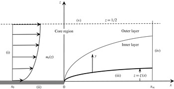
We examine the influence of finite slip in the visco-inertial regime, on an incompressible free-surface steady symmetric jet exiting a channel. Regardless of the level of slip, the emerging liquid jet experiences a sudden streamwise drop in shear stress at the channel exit between the solid wall and the jet free surface. This discontinuity is caused by the change in the boundary condition at the exit of the channel, where a partial slip condition is replaced by a free-surface condition. As a result, a boundary layer emanates from the channel exit, ensuring the lateral diffusion of vorticity, as illustrated in figure 1. Asymptotic development of the flow field is sought to handle the stress singularity at the channel exit, with the inverse power of the Reynolds number being the small parameter. Aside from the intrinsic importance of inertia in channel flow, additional inertial effect results from the significant elongation rate caused by the change (jump) in streamwise velocity at the channel exit. The connection with microchannel and hydrophobic flows is emphasized.
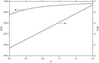
When a liquid flows on a solid surface, it is assumed to adhere to the solid surface as a result of viscous dissipation caused by the small-scale surface roughness and the adhesion between the liquid molecules and the solid surface. This is the prevalent assumption under normal flow circumstances, with the no-slip condition assumed at the solid wall. Therefore, this assumption can be expected to break down whenever the roughness scale is relatively large, as in a microchannel, or if the surface energy is relatively low. In such situations, the nature of the boundary condition changes from no slip (stick) to slip. One also refers to apparent slip when, for instance, the core fluid is flowing on a thin layer, with the latter adhering to the solid surface (Tretheway & Meinhart Reference Tretheway and Meinhart2004; Neto et al.
Reference Neto, Evans, Bonaccurso, Butt and Craig2005). The amount of slippage is represented by a slip length, which is the distance inside the solid at which the extrapolated flow profile equals zero (Lauga, Brenner & Stone Reference Lauga, Brenner, Stone, Foss, Tropea and Yarin2005). Even though these are typically in submicron scale, slip lengths as large as
 $20~{\rm\mu}\text{m}$
have been reported on superhydrophobic surfaces (Rothstein Reference Rothstein2010). In an ideal case, the slip length is directly proportional to the thickness of the plastron (thin air layer), making it possible to design extremely slippery surfaces (Choi & Kim Reference Choi and Kim2006).
Schematic illustration of free-surface jet (dimensionless notations used).

Slip is accounted for by assuming the tangential fluid velocity component at the solid surface to be proportional to the strain rate. Although the slip length may depend on shear rate (Choi, Westin & Breuer Reference Choi, Westin and Breuer2003), most molecular dynamic simulations seem to suggest that the slip length is an intrinsic property of the flowing liquid and the solid surface (Lauga et al. Reference Lauga, Brenner, Stone, Foss, Tropea and Yarin2005). The slip length will be assumed constant in the current study. Other factors known to affect slip include surface roughness (Zhu & Granick Reference Zhu and Granick2002), and dissolved gases and bubbles in the working fluid (Granick & Lee Reference Granick, Zhu and Lee2003). For a general perspective on slip and various mechanisms, the reader is referred to the review of Lauga et al. (Reference Lauga, Brenner, Stone, Foss, Tropea and Yarin2005).
Microchannel flows are typically characterized by small values of the Reynolds number. However, the exit flow in the current problem, like entry flow, involves an important (streamwise) elongation rate as a result of flow development. Elongation rate (as opposed to shear rate) is the reflection of the change in velocity with respect to the flow direction, thus leading to a significant convective or inertia effect. For this reason, entry flows, even in microchannels, are typically characterized by a significant inertia effect (see, for instance, Chakraborty & Anand (Reference Chakraborty and Anand2008), Duan & Muzychka (Reference Duan and Muzychka2010) and the references therein). Consequently, the current study focuses on the crucial interplay between slip and inertia effects given its criticality to developing microchannel and hydrophobic flows. Since hydrophobic interactions at the solid–fluid interface are attributed to surface heterogeneities, the resulting slippage is ascribed to the presence of amounts of gas trapped on the rough surface, typically in the form of microbubbles, or a gas layer at the solid surface (Lauga & Brenner Reference Lauga and Brenner2004). Chakraborty & Anand (Reference Chakraborty and Anand2008) examined theoretically the effect of such layer of gas and the resulting slip on the bulk flow in the entry region of a channel. In particular, they found that the presence of seemingly insignificantly small slip results in a dramatic change in flow behaviour. It is therefore crucial to understand how and if such a dramatic change can occur for the current exiting jet problem.
The present treatment follows that of adhering Newtonian (Tillett Reference Tillett1968; Miyake, Yukai & Iemoto Reference Miyake, Yukai and Iemoto1979; Philippe & Dumargue Reference Philippe and Dumargue1991) and non-Newtonian (Saffari & Khayat Reference Saffari and Khayat2009; Khayat Reference Khayat2014) jets. The treatment presents challenges due to the stress singularity, which is also encountered in other free-surface flows such as impinging jets (Bowles & Smith Reference Bowles and Smith1992; Phares, Smedley & Flagan Reference Phares, Smedley and Flagan2000; Bush & Aristoff Reference Bush and Aristoff2003), gravity-driven jets (Ruschak & Scriven Reference Ruschak and Scriven1977) and wall jets (Weinstein & Ruschak Reference Weinstein and Ruschak2004). The stress singularity constitutes the major difficulty in any theoretical analysis of these flows, especially numerical simulation. In contrast to localised asymptotic treatment, in a conventional numerical approach, the incorporation of the singularity point and its immediate vicinity, which is crucial for determining the flow field elsewhere, remains elusive. Perhaps, more importantly, asymptotic analyses tend to provide a deeper physical understanding of the flow structure near the singularity. In this regard, the current flow presents striking similarity with channel and conduit entry flows (Chakraborty & Anand Reference Chakraborty and Anand2008; Duan & Muzychka Reference Duan and Muzychka2010). This similarity is emphasized in the next section as we compare the influence of slip on existing entry flow with current exit flow findings.
For free-surface jet flow, asymptotic analysis has been successfully adopted in the visco-inertial range (Tillett Reference Tillett1968; Miyake et al. Reference Miyake, Yukai and Iemoto1979; Philippe & Dumargue Reference Philippe and Dumargue1991) and visco-capillary range (Goren & Wronski Reference Goren and Wronski1966; Ruschak & Scriven Reference Ruschak and Scriven1977). Tillett (Reference Tillett1968) analysed the laminar free jet flow near the channel exit, using the method of matched asymptotic expansions. Miyake et al. (Reference Miyake, Yukai and Iemoto1979) carried out a similar analysis for a vertical jet of an inviscid fluid, taking into account gravity effect. Philippe & Dumargue (Reference Philippe and Dumargue1991) also applied a similar approach for a viscous axisymmetric vertical jet, emphasizing the interplay between gravity and inertia. They validated the matched asymptotic approach against their measurements of velocity and jet profile. A local similarity transformation was carried out by Wilson (Reference Wilson1986) for the axisymmetric viscous-gravity jet of the boundary-layer type close to the free surface. The parallel between shear thinning (Khayat Reference Khayat2014) and slip will be highlighted throughout the current work.
In his book on interactive boundary-layer and triple-deck theories, Sobey (Reference Sobey2005) provides a recent perspective on asymptotic analyses, their applications and historic development. Incidentally, a triple-deck approach is not exactly applicable for the current problem, given the absence of an inviscid (external) layer. A closer treatment would be that of Smith (Reference Smith1979) on the flow in a tube with severe (axisymmetric) constriction. Smith observed that a model similar to the triple-deck formulation, based on an inviscid rotational core flow region, together with a viscous boundary-layer region near the wall, could be applied to the flow in the vicinity of the constriction. Similarly, a classical boundary-layer analysis is developed in the present problem near the free surface, and the boundary-layer flow is matched to the inviscid flow in the core region near the jet centreline. The flow field is thus determined at a small distance downstream of the jet.
In boundary-layer analysis, the solution is not valid within a small distance from inception, such as very near a leading edge or a stagnation point for an impinging jet (Zhao & Khayat Reference Zhao and Khayat2008). Similarly, the current analysis excludes the flow at the channel exit, between the wall and free surface. However, the distance in question is small, on the order of the (local) boundary-layer thickness, which is expected to be even smaller for a slipping jet. Consequently, the boundary-layer approach turns out to be successful in capturing the flow nature near the channel exit. Recall that the similarity character of the flow in the layer near the jet surface does not in fact require the upstream and downstream flows to match at the channel exit near the wall. Matching is required only in the core layer far from the wall. For an adhering jet, the flow is represented in terms of orthogonal functions, valid inside and outside the channel. This is not the case for a slipping jet where, as we shall see, the eigenmodes are different in the two regions due to the difference in the type of boundary conditions imposed inside and outside the channel.
2 Problem statement and formulation
Consider the steady symmetric two-dimensional flow of a free-surface incompressible jet, of density
 ${\it\rho}$
and viscosity
 ${\it\mu}$
, emerging from a channel of width
 $D$
. The different flow regions for the free-surface jet are illustrated schematically in figure 1, using dimensionless notations (to be introduced shortly). In each region, different physical mechanisms dominate the flow, with corresponding characteristic length scales. In particular, for the flow outside the channel, the region close to the free surface, the inner layer, is shear dominated and the flow is of the boundary-layer type. In the region between the inner layer and the centreline, the outer layer, both shear and elongation prevail as a result of the predominance of the Poiseuille character of the flow and the contracting jet. The outer layer extends to the channel interior and is part of the core region. The current flow problem is similar to entry flow of a slipping fluid in microconduits and channels where two main distinct regions are identified, consisting of an inviscid region (equivalent to the core region in figure 1) and a developing boundary layer that emanates from the entry point (Chakraborty & Anand Reference Chakraborty and Anand2008; Duan & Muzychka Reference Duan and Muzychka2010).
At large Reynolds number, the upstream diffusion of vorticity from the channel exit is small, and the distortion of the original parallel streamlines is also small. The vorticity generated at the trailing edge of the channel, where the stress singularity occurs, diffuses laterally, and is convected downstream, eventually contaminating the jet over a distance or relaxation length which turns out to be
 $O(Re)$
for both Newtonian (Tillett Reference Tillett1968) and shear-thinning fluids (Khayat Reference Khayat2014), but with a different definition of
 $Re$
in each case. This relaxation length is expected to depend strongly on the slip length (see § 5).
For a slipping fluid, the boundary-layer thickness is expected to decrease with slip length. In the inviscid limit, no boundary layer forms since there is no (viscous) mechanism for the stress singularity to diffuse, and all the conditions of the problem would be satisfied by postulating that the fully developed profile continues unchanged in the jet region, as for the case of wall-adhering jet flow (Tillett Reference Tillett1968). It is important to recall that no uniqueness theorem exists for this inviscid problem (Euler’s equations), and it is assumed that the fully developed Poiseuille flow for the slipping jet is everywhere the proper inviscid limit (see also Saffari & Khayat (Reference Saffari and Khayat2009) and Khayat (Reference Khayat2014) for the visco-elastic and power-law fluids, respectively). With this assumption, the flow in the core of the jet, to lowest order, is not affected by the flow in the boundary-layer region near the free surface, although the boundary layer is expected to induce perturbations to the base Poiseuille flow when higher-order terms are included, both for the flow upstream and downstream from the channel exit. This assumption was validated by Philippe & Dumargue (Reference Philippe and Dumargue1991) for an adhering jet, who extended Tillett’s formulation to include gravity for an axisymmetric jet emerging from a vertical tube. They also conducted measurements of the jet profile for different inertia-to-gravity forces, as well as the velocity profile at different positions inside and outside the tube for a jet of aqueous glycerine solution emerging out of a tube of few millimetres in diameter. Comparison between theory and experiment led to excellent agreement. This assumption is similar to the one made by Smith (Reference Smith1979) for the tube flow with severe constriction, where the flow field in the core region, to leading order, satisfies the inviscid equations of motion. Further discussion and comparison between the current and Smith’s formulations are given in § 4.
Far upstream, inside the channel, the flow is assumed to be fully developed, induced by a constant pressure gradient
 $G$
, and slipping at the solid boundaries. The problem is cast in terms of dimensionless variables and parameters. For this,
 $D$
,
 $V$
and
 ${\it\rho}V^{2}$
will be taken as the length, velocity and pressure scales, respectively. Here,
 $V$
is taken to correspond to the velocity at the centreline,
 $V=GD^{2}/8{\it\mu}$
, in the absence of slip, which turns out to be a suitable velocity scale for the problem. The flow configuration is schematically depicted in figure 1, in the
 $(x,z)$
plane. The
 $x$
-axis is taken along the channel wall, and the
 $z$
-axis is chosen in the transverse direction across the channel. The channel exit coincides with
 $x=0$
. In this case,
 $u$
and
 $w$
are the corresponding dimensionless velocity components. The velocity at the wall undergoes a first-order slip, with slip length-to-gap ratio denoted by
 $S$
. In this case,
 $u(x,z=0)=S(\partial u/\partial z)(x,z=0)$
. Thus,
 $S$
is defined such that a linear extrapolation of the velocity based on the gradient at the wall vanishes at
 $z=-S$
. Far upstream, the Poiseuille flow is the leading-order solution, and the velocity and the stream function are conveniently introduced here as
 $$\begin{eqnarray}\displaystyle & \displaystyle u(x,z)\sim u_{0}(z)\equiv 4(S+z-z^{2}),\quad \text{as }x\rightarrow -\infty , & \displaystyle\end{eqnarray}$$
 $$\begin{eqnarray}\displaystyle & \displaystyle {\it\psi}(x,z)\sim {\it\psi}_{0}(z)\equiv 4Sz+2z^{2}-{\textstyle \frac{4}{3}}z^{3},\quad \text{as }x\rightarrow -\infty . & \displaystyle\end{eqnarray}$$
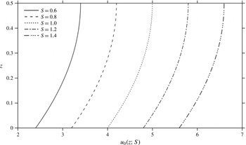
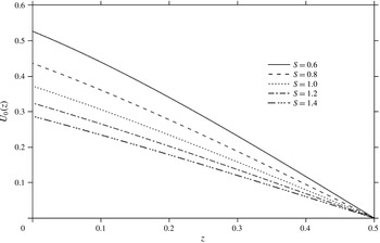
Fully developed velocity profiles for slip parameter range
 $S\in [0.6,1.4]$
. Values of
 $S$
shown will be used subsequently to illustrate the dependence of the flow on
 $S$
.

For reference, the Poiseuille velocity profiles are reported in figure 2 for
 $S\in [0.6,1.4]$
, which is the interval of interest in this study. The problem is conveniently formulated in terms of the stream function, introduced through
 $u={\it\psi}_{z}$
and
 $w=-{\it\psi}_{x}$
, and the governing equations become
 $$\begin{eqnarray}\displaystyle & \displaystyle Re({\it\psi}_{z}{\it\psi}_{xz}-{\it\psi}_{x}{\it\psi}_{zz})=-Re\,p_{x}+{\it\psi}_{xxz}+{\it\psi}_{zzz}, & \displaystyle\end{eqnarray}$$
 $$\begin{eqnarray}\displaystyle & \displaystyle Re({\it\psi}_{x}{\it\psi}_{xz}-{\it\psi}_{z}{\it\psi}_{xx})=-Re\,p_{z}-{\it\psi}_{xxx}-{\it\psi}_{xzz}. & \displaystyle\end{eqnarray}$$
 $x$
and
 $z$
denote partial differentiation. For
 $x>0$
, the (lower) jet height is denoted by
 $z={\it\zeta}(x)$
. Noting that the (dimensionless) stress matrix at any point is
 $\left(\!\begin{smallmatrix}-Re\,p+2{\it\psi}_{zx} & {\it\psi}_{zz}-{\it\psi}_{xx}\\ {\it\psi}_{zz}-{\it\psi}_{xx} & -Re\,p-2{\it\psi}_{zx}\end{smallmatrix}\!\right)$
and the normal to the jet surface is
 $\left(\begin{smallmatrix}{\it\zeta}^{\prime }\\ -1\end{smallmatrix}\right)$
, then the kinematic and dynamic boundary conditions at the jet surface become (assuming negligible surface tension effect)
 $$\begin{eqnarray}\displaystyle & \displaystyle {\it\psi}(x>0,z={\it\zeta})=0, & \displaystyle\end{eqnarray}$$
 $$\begin{eqnarray}\displaystyle & \displaystyle p(x>0,z={\it\zeta}){\it\zeta}^{\prime }-Re^{-1}\left.(2{\it\zeta}^{\prime }{\it\psi}_{xz}+{\it\psi}_{xx}-{\it\psi}_{zz})\right|_{x>0,z={\it\zeta}}=0, & \displaystyle\end{eqnarray}$$
 $$\begin{eqnarray}\displaystyle & \displaystyle p(x>0,z={\it\zeta})+Re^{-1}[2{\it\psi}_{xz}+{\it\zeta}^{\prime }({\it\psi}_{zz}-{\it\psi}_{xx})]_{x>0,z={\it\zeta}}=0, & \displaystyle\end{eqnarray}$$
 $x$
(or
 $z$
). Inside the channel
 $(x<0)$
, the following conditions must be satisfied, namely,
 $$\begin{eqnarray}\displaystyle & \displaystyle {\it\psi}\left(x\leqslant 0,z=\frac{1}{2}\right)=\frac{6S+1}{3}, & \displaystyle\end{eqnarray}$$
 $$\begin{eqnarray}\displaystyle & \displaystyle {\it\psi}(x\leqslant 0,z=0)=0, & \displaystyle\end{eqnarray}$$
 $$\begin{eqnarray}\displaystyle & \displaystyle {\it\psi}_{z}(x\leqslant 0,z=0)=S{\it\psi}_{zz}(x\leqslant 0,z=0), & \displaystyle\end{eqnarray}$$
 $$\begin{eqnarray}\displaystyle & \displaystyle {\it\psi}(x,z)\sim 4Sz+2z^{2}-{\textstyle \frac{4}{3}}z^{3},\quad \text{as }x\rightarrow -\infty . & \displaystyle\end{eqnarray}$$
 $S=O(1)$
, implying a relatively large slip length, which is not uncommon for superhydrophobic surfaces (Rothstein Reference Rothstein2010). Large slip length is detected in the presence of an air–water interface in microridges. Ou & Rothstein (Reference Ou and Rothstein2005) used
 ${\it\mu}$
-PIV measurements to examine the flow kinematics in a microchannel at length scales well below that of the microridges on the superhydrophobic surface. The flow was observed to come to rest along the microridges but slip velocities greater than 60 % of the average velocity were detected along the air–water interface. In this case, since the average velocity, based on (2.1), is given by
 $(2/3)(6S+1)$
, then
 $S=0.25$
.
When the free-surface jet emerges at the channel exit
 $(x=0)$
, the shear stress undergoes a step change from a non-zero value at the wall
 $(z=0)$
, to zero at the free surface,
 $z={\it\zeta}(x)$
. Note from (2.1) that the wall shear stress is equal to 4, and is independent of slip length. As the fluid detaches itself from the wall of the channel, the removal of the wall stress causes a boundary layer to form in a region near the free surface. In this region, the base velocity profile adjusts itself so as to satisfy the condition of zero traction at the free surface.
The effect of the drop in shear stress diffuses upstream inside the channel
 $(x<0)$
over a distance
 $x_{0}$
where fully developed Poiseuille flow prevails, and downstream
 $(x>0)$
toward the centreline over a distance
 $x_{\infty }$
, and the original Poiseuille flow gradually acquires a boundary-layer character. The flow is thus supposed to have the base Poiseuille profile (2.2) to lowest order, and is modified when the fluid approaches the channel exit and leaves the channel. The asymptotic analysis circumvents the singularity by identifying two distinct flow regions: a boundary-layer region near the free surface, extending but not including the singular point, and a core region where the flow remains close to fully developed (see figure 1). As in any boundary-layer flow, the inclusion of the singularity is not required in this case given the similarity character of the flow near the free surface. Although this boundary-layer region extends both upstream and downstream from the singularity, the flow does not remain fully developed as it approaches the exit, but the thickness of the boundary layer upstream of the exit is generally small at high Reynolds number, particularly for slipping flow, and is therefore ignored (Tillett Reference Tillett1968).
The current study focuses on the flow outside the channel where the similarity solution in the inner layer is matched onto the outer solution. In addition, the solution in the outer layer outside the channel must match that inside the channel at the channel exit. It is emphasised that no matching is required for the similarity solution at
 $x=0$
, and the flow singularity at the origin is entirely avoided in the solution process. This constitutes the major advantage of the current formulation, which is closely related to the ideas advanced in Stewartson’s triple-deck theory (Sobey Reference Sobey2005). The theory examines flow separation and other nonlinear features in external flow situations. The fundamental difference between the external separation phenomenon and the current jet flow through a channel is the absence of an external inviscid region in the current case, although the core layer is of inviscid but rotational character (see figure 1). The current approach follows more closely that of Smith (Reference Smith1976a
,Reference Smith
b
, Reference Smith1979), who examined the fully developed flow through an indented tube when the Reynolds number is large. As in the current problem, there is no external flow region, and the triple-deck formulation could not simply be carried over to Smith’s problem, but, as with the current jet problem, Smith realized that a model based on an inviscid rotational core flow region together with viscous boundary-layer regions near the walls could be applied to his problem. However, as we shall see, the presence of slip adds a significant challenge in the matching process at the channel exit
 $(x=0)$
as well as at the inner–outer-layer interface.
The problem is next examined by considering separately the flow near the free surface (inner layer) in § 3, and the flow in the core region (outer layer) is introduced in § 4, along with the establishment of the boundary conditions needed to determine the flow in the core layer. Some of these conditions are generated by asymptotic matching between the inner and outer layers. Section 5 is devoted to the solution of the outer core layer inside and outside the channel, and the determination of the jet profile. The composite flow is obtained in § 6 by merging the inner and outer solutions. Finally, an integral formulation is presented in § 7, which highlights the influence of slip on the jet contraction ratio and speed. Discussion and concluding remarks are given in § 8.
3 Flow near the jet surface
Close to the jet surface, in the inner layer, the flow is of the boundary-layer type. A hierarchy of equations and boundary conditions are generated that admit a similarity solution to each order. The influence of slip on boundary-layer growth is closely examined.
3.1 Flow in the inner layer (near the jet surface)
To examine the boundary-layer structure near the free surface, let
 $y=z-{\it\zeta}(x)$
. The scaling in the transverse direction is changed by writing
 $y={\it\varepsilon}{\it\eta}$
, where
 ${\it\varepsilon}$
is the small parameter in the problem, defined as
 ${\it\varepsilon}=Re^{-{\it\alpha}}$
(or
 $Re={\it\varepsilon}^{-1/{\it\alpha}}$
), where
 ${\it\alpha}$
is to be determined. Anticipating that the height
 ${\it\zeta}$
of the free surface is of the same order of magnitude as the boundary-layer thickness, one can write
 ${\it\zeta}(x)={\it\varepsilon}h(x)$
, and henceforth work with
 $h(x)$
. Following Tillett (Reference Tillett1968) and Philippe & Dumargue (Reference Philippe and Dumargue1991), the following change of coordinates is introduced, namely,
 $$\begin{eqnarray}x={\it\xi},\quad z={\it\varepsilon}({\it\eta}+h).\end{eqnarray}$$
The aim is to find a solution of the transformed problem (2.3)–(2.5) in the form of an inner expansion in
 ${\it\varepsilon}$
. In order to match this to the outer Poiseuille flow, it is necessary to have
 ${\it\psi}\sim {\it\varepsilon}{\it\eta}=y$
as
 ${\it\eta}\rightarrow \infty$
in the inner region, to lowest order in
 ${\it\varepsilon}$
; so
 ${\it\psi}$
must be of order
 ${\it\varepsilon}$
.
In order to determine the value of
 ${\it\alpha}$
, it is required that the convective and viscous terms balance in the governing equations. The balance in the boundary conditions simply follows. The transformed equations and boundary conditions are given in appendix A. Recalling that
 ${\it\psi}=O({\it\varepsilon})$
, the force balance in (A 1) is ensured upon taking
 ${\it\alpha}=1/2$
. Consequently,
 $Re={\it\varepsilon}^{-2}$
or
 ${\it\varepsilon}=Re^{-1/2}$
, which signals the major departure from previous formulations where
 ${\it\alpha}=1/3$
for non-slipping Newtonian (Tillett Reference Tillett1968; Philippe & Dumargue Reference Philippe and Dumargue1991) and non-Newtonian (Saffari & Khayat Reference Saffari and Khayat2009; Khayat Reference Khayat2014) jets.
Consequently, the problem in the inner layer reduces to
 $$\begin{eqnarray}\displaystyle & & \displaystyle \displaystyle {\it\psi}_{{\it\eta}}{\it\psi}_{{\it\xi}{\it\eta}}-{\it\psi}_{{\it\xi}}{\it\psi}_{{\it\eta}{\it\eta}}=-{\it\varepsilon}^{2}(p_{{\it\xi}}-h^{\prime }p_{{\it\eta}})+{\it\varepsilon}{\it\psi}_{{\it\eta}{\it\eta}{\it\eta}}+{\it\varepsilon}^{3}({\it\psi}_{{\it\xi}{\it\xi}{\it\eta}}-h^{\prime \prime }{\it\psi}_{{\it\eta}{\it\eta}}-2h^{\prime }{\it\psi}_{{\it\xi}{\it\eta}{\it\eta}}+h^{\prime 2}{\it\psi}_{{\it\eta}{\it\eta}{\it\eta}}),\nonumber\\ \displaystyle & & \displaystyle\end{eqnarray}$$
 $$\begin{eqnarray}\displaystyle & & \displaystyle \displaystyle -{\it\psi}_{{\it\eta}}{\it\psi}_{{\it\xi}{\it\xi}}+{\it\psi}_{{\it\xi}}{\it\psi}_{{\it\xi}{\it\eta}}+h^{\prime \prime }{\it\psi}_{{\it\eta}}^{2}+h^{\prime }({\it\psi}_{{\it\eta}}{\it\psi}_{{\it\xi}{\it\eta}}-{\it\psi}_{{\it\xi}}{\it\psi}_{{\it\eta}{\it\eta}})\nonumber\\ \displaystyle & & \displaystyle \displaystyle \qquad =-p_{{\it\eta}}-{\it\varepsilon}({\it\psi}_{{\it\xi}{\it\eta}{\it\eta}}-h^{\prime }{\it\psi}_{{\it\eta}{\it\eta}{\it\eta}})-{\it\varepsilon}^{3}\left(\frac{\partial }{\partial {\it\xi}}-h^{\prime }\frac{\partial }{\partial {\it\eta}}\right)^{3}{\it\psi},\end{eqnarray}$$
 $$\begin{eqnarray}\displaystyle & \displaystyle {\it\psi}({\it\xi},{\it\eta}=0)=0, & \displaystyle\end{eqnarray}$$
 $$\begin{eqnarray}\displaystyle & \displaystyle {\it\varepsilon}h^{\prime }p({\it\xi},{\it\eta}=0)+[(1+{\it\varepsilon}^{2}h^{\prime 2}){\it\psi}_{{\it\eta}{\it\eta}}+{\it\varepsilon}^{2}h^{\prime \prime }{\it\psi}_{{\it\eta}}]_{{\it\xi},{\it\eta}=0}=0, & \displaystyle\end{eqnarray}$$
 $$\begin{eqnarray}\displaystyle & \displaystyle p({\it\xi},{\it\eta}=0)+{\it\varepsilon}[2(1+{\it\varepsilon}^{2}h^{\prime 2}){\it\psi}_{{\it\xi}{\it\eta}}-h^{\prime }(1+{\it\varepsilon}^{2}h^{\prime 2}){\it\psi}_{{\it\eta}{\it\eta}}+{\it\varepsilon}^{2}h^{\prime }h^{\prime \prime }{\it\psi}_{{\it\eta}}]_{{\it\xi},{\it\eta}=0}=0. & \displaystyle\end{eqnarray}$$
 ${\it\psi}$
begins with a term in
 ${\it\varepsilon}$
. This is assumed, until there is evidence to the contrary. Thus, the expansion proceeds in powers of
 ${\it\varepsilon}$
so that
 $$\begin{eqnarray}{\it\psi}({\it\xi},{\it\eta})={\it\varepsilon}{\it\Psi}_{1}({\it\xi},{\it\eta})+{\it\varepsilon}^{2}{\it\Psi}_{2}({\it\xi},{\it\eta})+{\it\varepsilon}^{3}{\it\Psi}_{3}({\it\xi},{\it\eta})+\cdots \,.\end{eqnarray}$$
Similarly,
 $h$
is expanded as
 $$\begin{eqnarray}h({\it\xi})={\it\varepsilon}^{-1}{\it\zeta}({\it\xi})=h_{0}({\it\xi})+{\it\varepsilon}h_{1}({\it\xi})+\cdots \,.\end{eqnarray}$$
As to the pressure, (3.2b
) and condition (3.3c
) lead to
 $P_{0{\it\eta}}({\it\xi},{\it\eta})=0$
and
 $P_{0}({\it\xi},{\it\eta}=0)=0$
, respectively. Thus,
 $P_{0}({\it\xi},{\it\eta})=0$
everywhere. Similarly,
 $P_{1{\it\eta}}({\it\xi},{\it\eta})=0$
and
 $P_{1}({\it\xi},{\it\eta}=0)=0$
, leading to
 $P_{1}({\it\xi},{\it\eta})=0$
. Thus, it is concluded that the pressure in the inner layer is of order
 ${\it\varepsilon}^{2}$
, and
 $$\begin{eqnarray}p({\it\xi},{\it\eta})={\it\varepsilon}^{2}P_{2}({\it\xi},{\it\eta})+{\it\varepsilon}^{3}P_{3}({\it\xi},{\it\eta})+\cdots \,.\end{eqnarray}$$
The streamwise and transverse velocity components are now expressed as
 $u=(1/{\it\varepsilon}){\it\psi}_{{\it\eta}},w=-{\it\psi}_{{\it\xi}}+h^{\prime }{\it\psi}_{{\it\eta}}$
. It is obvious that
 $u=O(1)$
, which is also confirmed by considering the fact that
 $u$
in the inner region must match the velocity in the outer region:
 $u\rightarrow 4(S+z-z^{2})$
, and we must have
 $u\sim 4S$
as
 ${\it\eta}\rightarrow \infty$
. Clearly,
 $w$
is of order
 ${\it\varepsilon}$
. In this case, the velocity components take the form:
 $$\begin{eqnarray}\displaystyle & \displaystyle u({\it\xi},{\it\eta})=U_{0}({\it\xi},{\it\eta})+{\it\varepsilon}U_{1}({\it\xi},{\it\eta})+\cdots \,, & \displaystyle\end{eqnarray}$$
 $$\begin{eqnarray}\displaystyle & \displaystyle w({\it\xi},{\it\eta})={\it\varepsilon}W_{1}({\it\xi},{\it\eta})+{\it\varepsilon}^{2}W_{2}({\it\xi},{\it\eta})+\cdots \,. & \displaystyle\end{eqnarray}$$
Here,
 $U_{0}={\it\Psi}_{1{\it\eta}},W_{1}=-{\it\Psi}_{1{\it\xi}}+h_{0}^{\prime }{\it\Psi}_{1{\it\eta}},U_{1}={\it\Psi}_{2{\it\eta}}$
, etc.
To leading order, (3.2a ) and (3.2b ) reduce, respectively, to
 $$\begin{eqnarray}\displaystyle & \displaystyle {\it\Psi}_{1{\it\eta}}{\it\Psi}_{1{\it\xi}{\it\eta}}-{\it\Psi}_{1{\it\xi}}{\it\Psi}_{1{\it\eta}{\it\eta}}={\it\Psi}_{1{\it\eta}{\it\eta}{\it\eta}}, & \displaystyle\end{eqnarray}$$
 $$\begin{eqnarray}\displaystyle & \displaystyle -{\it\psi}_{1{\it\eta}}{\it\psi}_{1{\it\xi}{\it\xi}}+{\it\psi}_{1{\it\xi}}{\it\psi}_{1{\it\xi}{\it\eta}}+h_{0}^{\prime \prime }{\it\psi}_{1{\it\eta}}^{2}+h_{0}^{\prime }({\it\psi}_{1{\it\eta}}{\it\psi}_{1{\it\xi}{\it\eta}}-{\it\psi}_{1{\it\xi}}{\it\psi}_{1{\it\eta}{\it\eta}})=-p_{2{\it\eta}}-({\it\psi}_{1{\it\xi}{\it\eta}{\it\eta}}-h_{0}^{\prime }{\it\psi}_{1{\it\eta}{\it\eta}{\it\eta}}). & \displaystyle \nonumber\\ \displaystyle & & \displaystyle\end{eqnarray}$$
 $$\begin{eqnarray}\displaystyle & \displaystyle {\it\Psi}_{1}({\it\xi},{\it\eta}=0)={\it\Psi}_{1{\it\eta}{\it\eta}}({\it\xi},{\it\eta}=0)=0, & \displaystyle\end{eqnarray}$$
 $$\begin{eqnarray}\displaystyle & \displaystyle P_{2}({\it\xi},{\it\eta}=0)=-2{\it\Psi}_{1{\it\xi}{\it\eta}}({\it\xi},{\it\eta}=0). & \displaystyle\end{eqnarray}$$
 ${\it\Psi}_{1}$
, another boundary condition is required. This is the matching condition at the edge of the inner layer, which will be obtained in appendix C from (C 6), namely
 $$\begin{eqnarray}{\it\Psi}_{1}({\it\xi},{\it\eta})\sim 4S{\it\eta},\quad \text{as }{\it\eta}\rightarrow \infty .\end{eqnarray}$$
Clearly,
 ${\it\Psi}_{1}({\it\xi},{\it\eta})=4S{\it\eta}$
is the solution to this order. In this case,
 $P_{2}({\it\xi},{\it\eta}=0)=0$
. Consequently, the pressure gradient is given by
 $P_{2{\it\eta}}({\it\xi},{\it\eta})=-h_{0}^{\prime \prime }{\it\Psi}_{1{\it\eta}}^{2}=-16S^{2}h_{0}^{\prime \prime }$
, and
 $P_{2}({\it\xi},{\it\eta})=-16S^{2}h_{0}^{\prime \prime }{\it\eta}$
. Formally, the leading-order terms are
 $$\begin{eqnarray}{\it\Psi}_{1}({\it\xi},{\it\eta})=4S{\it\eta},\quad P_{2}({\it\xi},{\it\eta})=-16S^{2}h_{0}^{\prime \prime }{\it\eta}.\end{eqnarray}$$
To
 $O({\it\varepsilon}^{2})$
, using solution (3.12), (3.2a
) and boundary conditions (3.3) lead to
 $$\begin{eqnarray}4S{\it\Psi}_{2{\it\xi}{\it\eta}}={\it\Psi}_{2{\it\eta}{\it\eta}{\it\eta}},\quad {\it\Psi}_{2}({\it\xi},{\it\eta}=0)={\it\Psi}_{2{\it\eta}{\it\eta}}({\it\xi},{\it\eta}=0)=0.\end{eqnarray}$$
The solution of this problem is given in appendix B. The asymptotic form of
 ${\it\Psi}_{2}$
is obtained from (B 4) to read
 $$\begin{eqnarray}{\it\Psi}_{2}({\it\xi},{\it\eta})\sim 2{\it\eta}^{2}+\frac{{\it\xi}}{S},\quad \text{as }{\it\eta}\rightarrow \infty .\end{eqnarray}$$
This relation is sufficient to determine the shape of the jet surface in the matching process of § 4. However, the velocity along the jet surface becomes only available from the full solution of problem (3.13)–(3.14), which is outlined in appendix B. To this order, the velocity field in the inner layer is determined by recalling (3.4), (3.7) and (3.8), leading to
 $$\begin{eqnarray}\displaystyle & \displaystyle {\it\psi}({\it\xi},{\it\eta})=4{\it\varepsilon}S{\it\eta}+{\it\varepsilon}^{2}{\it\xi}f_{2}({\it\theta})+O({\it\varepsilon}^{3}), & \displaystyle\end{eqnarray}$$
 $$\begin{eqnarray}\displaystyle & \displaystyle u({\it\xi},{\it\eta})=4S+{\it\varepsilon}{\it\xi}^{1/2}f_{2}^{\prime }({\it\theta})+O({\it\varepsilon}^{2}), & \displaystyle\end{eqnarray}$$
 $$\begin{eqnarray}\displaystyle & \displaystyle w({\it\xi},{\it\eta})=[4S+{\it\varepsilon}{\it\xi}^{1/2}f_{2}^{\prime }({\it\theta})]{\it\zeta}^{\prime }(x)+{\it\varepsilon}^{2}\left[\frac{{\it\theta}}{2}f_{2}^{\prime }({\it\theta})-f_{2}({\it\theta})\right]+O({\it\varepsilon}^{3}), & \displaystyle\end{eqnarray}$$
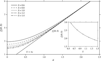
Influence of slip length on
 $f_{2}^{\prime }({\it\theta})$
for
 $Re=81$
, with the
 $S\rightarrow \infty$
curve also corresponding to the asymptotic behaviour for all
 $S$
. Inset depicts dependence of
 $f_{2}^{\prime }(0)$
on
 $S$
. Markers in the inset indicate the five cases emphasized throughout this study.

where
 $f_{2}({\it\theta})$
and
 $f_{2}^{\prime }({\it\theta})$
are recalled from (B 5a
) and (B 5b
), respectively. Figure 3 displays the influence of slip on
 $f_{2}^{\prime }({\it\theta})$
. The solution for large
 $S$
 $(S\rightarrow \infty )$
is also included, which constitutes the asymptotic behaviour
 $f_{2}^{\prime }({\it\theta})\sim 4{\it\theta}$
as
 ${\it\theta}\rightarrow \infty$
for any
 $S$
. The figure shows that
 $f_{2}^{\prime }({\it\theta})$
adjusts itself to the asymptotic linear behaviour at a shorter distance from the channel exit (origin) with increasing slip, reflecting a thinning of the boundary layer (see below). The curve saturation is also evident as
 $f_{2}^{\prime \prime }({\it\theta})$
reaches the constant level 4. Of particular interest is the dependence of
 $f_{2}^{\prime }({\it\theta}=0)$
on
 $S$
, which is related to the flow at the jet surface, and is easily determined from (3.15b
) upon recalling (B 5b
) and noting that
 $\text{erf}(x=0)=0$
. In this case:
 $$\begin{eqnarray}f_{2}^{\prime }({\it\theta}=0;S)=\frac{4}{\sqrt{{\rm\pi}S}}.\end{eqnarray}$$
Given its significance, this function is shown in the inset of figure 3. As discussed next, the decrease of
 $f_{2}^{\prime }({\it\theta}=0;S)$
with
 $S$
suggests a weakening of the flow perturbation along the jet surface with slip relative to the Poiseuille level.
Indeed, the flow along the jet surface, including the velocity and shear stress
 ${\it\tau}_{xz}={\it\psi}_{zz}-{\it\psi}_{xx}$
is given through the following expressions in terms of
 $Re$
and
 $S$
:
 $$\begin{eqnarray}\displaystyle & \displaystyle u(x,z={\it\zeta})=4\left(S+\sqrt{\frac{x}{{\rm\pi}S\,Re}}\right)+O(Re^{-1}), & \displaystyle\end{eqnarray}$$
 $$\begin{eqnarray}\displaystyle & \displaystyle w(x,z={\it\zeta})=4\left(S+\sqrt{\frac{x}{{\rm\pi}S\,Re}}\right){\it\zeta}^{\prime }(x)+O(Re^{-3/2}), & \displaystyle\end{eqnarray}$$
 $$\begin{eqnarray}\displaystyle & \displaystyle {\it\tau}_{xz}(x,z={\it\zeta})=4\sqrt{\frac{1}{{\rm\pi}Re\,Sx}}{\it\zeta}^{\prime }(x)+O(Re^{-1}). & \displaystyle\end{eqnarray}$$
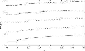
Streamwise velocity component as function of position along the jet surface for
 $Re=80$
and slip parameter range
 $S\in [0.6,1.4]$
. Also shown, is the level of velocity along the wall for each
 $S(x<0,z=0)$
. Curve legends are the same as in figure 3.

Figure 4 depicts the influence of slip on the streamwise velocity component along the jet surface for
 $Re=80$
. Also shown are the velocity levels at the wall, given by
 $u(x<0,z=0)=4S$
. The streamwise flow weakens relative to the velocity at the wall with increasing slip. Like inertia, slip helps retain the Poiseuille character of the jet, with the additional slippage along the jet surface behaving like
 $S^{-1/2}$
. As (3.17a
) suggests,
 $u({\it\xi},{\it\eta}=0)\sim 4S$
for large
 $S$
; there is no change in the flow field upon crossing the channel exit.
At this stage, the next order in the pressure contribution can be obtained by considering (3.2b ) and corresponding boundary conditions:
 $$\begin{eqnarray}P_{3{\it\eta}}={\it\Psi}_{1{\it\eta}}{\it\Psi}_{2{\it\xi}{\it\xi}}-h_{1}^{\prime \prime }{\it\Psi}_{1{\it\eta}}^{2}-{\it\Psi}_{2{\it\xi}{\it\eta}{\it\eta}},\quad P_{3}({\it\xi},{\it\eta}=0)+2{\it\Psi}_{2{\it\xi}{\it\eta}}({\it\xi},{\it\eta}=0)=0.\end{eqnarray}$$
Noting from (3.13) that
 ${\it\Psi}_{2{\it\eta}{\it\eta}}=4S{\it\Psi}_{2{\it\xi}}$
, and recalling from (3.12) that
 ${\it\Psi}_{1{\it\eta}}=4S$
, the pressure gradient in (3.18) reduces to
 $P_{3{\it\eta}}=-16S^{2}h_{1}^{\prime \prime }$
, to give
 $P_{3}({\it\xi},{\it\eta})=-16S^{2}h_{1}^{\prime \prime }{\it\eta}-2{\it\Psi}_{2{\it\xi}{\it\eta}}({\it\xi},{\it\eta}=0)$
. In this case, recalling the solution of problem (3.13), the pressure contribution to this order becomes
 $$\begin{eqnarray}p({\it\xi},{\it\eta})=-16{\it\varepsilon}^{2}S^{2}h_{0}^{\prime \prime }{\it\eta}-4{\it\varepsilon}^{3}\left(4S^{2}h_{1}^{\prime \prime }{\it\eta}+\frac{1}{\sqrt{{\rm\pi}S{\it\xi}}}\right).\end{eqnarray}$$
Of particular interest is the pressure at the free surface to this order, which is given by
 $$\begin{eqnarray}p(x,z={\it\zeta})=-\frac{4}{\sqrt{{\rm\pi}S\,Re^{3}x}}+O(Re^{-2}).\end{eqnarray}$$
Although the inner solution to next order is not needed, its asymptotic behaviour is still required to determine
 $h_{1}(x)$
. This contribution to the jet profile is crucial as
 $h_{0}(x)$
turns out to be zero (see § 4). Only the problem statement for
 ${\it\Psi}_{3}({\it\xi},{\it\eta})$
is given here, with the details given in appendix B. Thus, to
 $O({\it\varepsilon}^{3})$
, (3.2a
) reduces to
 $$\begin{eqnarray}{\it\Psi}_{1{\it\eta}}{\it\Psi}_{3{\it\xi}{\it\eta}}+{\it\Psi}_{2{\it\eta}}{\it\Psi}_{2{\it\xi}{\it\eta}}-{\it\Psi}_{2{\it\xi}}{\it\Psi}_{2{\it\eta}{\it\eta}}={\it\Psi}_{3{\it\eta}{\it\eta}{\it\eta}},\end{eqnarray}$$
subject to the boundary conditions deduced from (3.3a ) and (3.3b ), as well as the matching condition from (C 6), namely
 $$\begin{eqnarray}{\it\Psi}_{3}({\it\xi},{\it\eta}=0)=0,\quad {\it\Psi}_{3{\it\eta}{\it\eta}}({\it\xi},{\it\eta}=0)=4Sh_{0}^{\prime \prime },\quad {\it\Psi}_{3}({\it\xi},{\it\eta})\sim -{\textstyle \frac{4}{3}}{\it\eta}^{3}\quad \text{as }{\it\eta}\rightarrow \infty .\end{eqnarray}$$
More precisely, the asymptotic behaviour is (appendix B)
 $$\begin{eqnarray}{\it\Psi}_{3}({\it\xi},{\it\eta})\sim -\frac{4}{3}\left({\it\eta}^{3}+3\frac{(2S-1)}{4S^{2}}{\it\xi}{\it\eta}+d\right),\quad \text{as }{\it\eta}\rightarrow \infty .\end{eqnarray}$$
Here
 $d$
is a constant whose value is of no consequence to the order sought in the current study.
Influence of slip and inertia on boundary-layer height at
 $x=1$
: (a) streamwise velocity component is plotted against height in the inner layer for
 $Re=80$
, asymptotic (linear) behaviour is also shown for each slip level, (b) velocity at inner-layer edge for different Reynolds numbers. Inset shows the dependence of inner-layer height on
 $S$
.

3.2 Inner-layer growth
The inner-layer height is estimated by examining the variation of the velocity profile (3.15b
) with respect to
 ${\it\eta}$
(or
 ${\it\theta}$
) at a position
 $x$
relative to its asymptotic form. Thus, the inner-layer thickness is determined once
 ${\it\theta}={\it\theta}_{\infty }(Re,S)$
, which is defined through
 $(f_{2}^{\prime }({\it\theta}_{\infty })-4{\it\theta}_{\infty })/4{\it\theta}_{\infty }=1\,\%$
. Recalling (B 5b
), we obtain the following transcendental equation and solution for
 ${\it\theta}_{\infty }$
:
 $$\begin{eqnarray}\text{e}^{-S{\it\theta}_{\infty }^{2}}+[\text{erf}(\sqrt{S}{\it\theta}_{\infty })-1.01]\sqrt{{\rm\pi}S}\,{\it\theta}_{\infty }=0,\quad {\it\theta}_{\infty }=\frac{1.38}{\sqrt{S}}.\end{eqnarray}$$
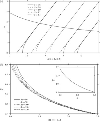
Figure 5 illustrates the influence of slip on velocity in the inner layer for
 $Re=80$
(figure 5
a) and the influence of inertia on boundary-layer height (figure 5
b) at
 $x=1$
. The asymptotic solution tends to underestimate the velocity level. The inner-layer height coincides with the level at which the asymptotic and inner velocity profiles begin to merge, corresponding to
 ${\it\eta}_{\infty }=1.38/\sqrt{S}$
. The locus of merging points is highlighted in figure 5(a). The loci at different Reynolds numbers are also plotted in figure 5(b), displaying the influence of inertia and slip on the velocity at the edge of the inner layer. Clearly, as the inset in figure 5(b) indicates, the inner-layer height decreases with slip, eventually vanishing for infinite slip length.
To leading order, (3.24) yields the inner-layer thickness as
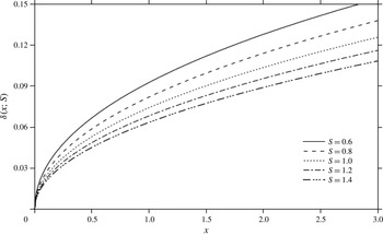
 ${\it\delta}(x;Re,S)=1.38\sqrt{x/S\,Re}$
. The boundary-layer thickness predominantly grows with position, at a rate that decreases with inertia and slip. As expected, the boundary layer vanishes in the limit of large
 $S$
; there is simply no discontinuity in shear stress. Incidentally, for gravity-driven jet flow Wilson (Reference Wilson1986), the boundary-layer height behaves like
 $(x/Re)^{1/4}$
, whereas for Newtonian (Tillett Reference Tillett1968) and non-Newtonian (Saffari & Khayat Reference Saffari and Khayat2009; Khayat Reference Khayat2014) jets, the boundary layer grows like
 $(x/Re)^{1/3}$
.
Generally, the stress singularity at the exit diffuses more slowly (over a longer distance) for the more slipping jet as a result of the thinner boundary layer. A similar argument holds for inertial effect. More precisely, since boundary-layer theory neglects viscous forces arising from streamwise velocity gradients, it must be expected to break down when shearing and elongation terms are of the same order of magnitude, that is when
 $\partial u/\partial x\simeq \partial u/\partial y$
, or when
 $x$
is of order
 ${\it\delta}$
. This leads to
 $x=O(1/S\,Re)$
, which means that the inner-layer solution never breaks down for an infinitely slipping jet! More realistically, the inner-layer solution remains valid, starting at a closer point to the channel exit, for a jet with larger slip length and Reynolds number.
Further correction is made by including the higher-order term. Upon balancing inertial and viscous terms in (3.2) and using the velocity at the jet surface (3.17a ), we have
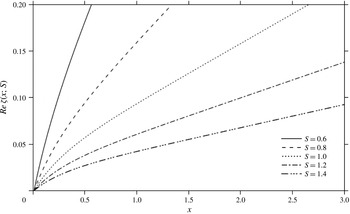
 $$\begin{eqnarray}{\it\delta}(x;Re,S)=1.38\sqrt{\frac{x}{S\,Re}}\left[1-\frac{1}{2S}\sqrt{\frac{x}{{\rm\pi}S\,Re}}\right]+O(Re^{-3/2}).\end{eqnarray}$$
The rate of decrease of inner-layer height with
 $Re$
and
 $S$
is clearly tempered by the higher-order term, pointing to the possibility of non-monotonic growth, in contrast to the case of an adhering jet. Figure 6 depicts the influence of slip on the boundary-layer profile. Note the significant jump in height for an adhering jet (see below for further discussion on this phenomenon). As the boundary layer grows with distance, it eventually invades the entire jet width, that is when
 ${\it\delta}\sim O(1)$
. Expression (3.25) indicates that this happens at a distance
 $x\sim S\,Re$
.
Finally, it is worth observing that, for an adhering jet, the boundary-layer assumption in the inner layer is valid at large Reynolds number; the boundary-layer equations are obtained from the Navier–Stokes equations by neglecting higher-order terms in the inverse of the Reynolds number. For slipping flow, the boundary-layer equations are expected to remain accurate even when the Reynolds number is only moderate. This extended range of validity is attributed to the decrease in viscous effect resulting from slip, which ensures that even moderate inertia remains relatively dominant for the boundary-layer equations to hold. Hence, the Reynolds number can be lower for the more slipping fluid for the boundary-layer equations to remain valid. The extended range of validity also holds for shear-thinning fluids (Khayat Reference Khayat2014), which was also confirmed by Wu & Thompson (Reference Wu and Thompson1996) in their comparison between experiment and numerical solution for the flow over a flat plate. In the current study, it is found that the inner-layer flow is accurate to
 $O(Re^{-1/2})$
for a slipping jet, and to
 $O(Re^{-1/3})$
for an adhering jet (Tillett Reference Tillett1968; Khayat Reference Khayat2014).
Influence of slip on boundary-layer thickness (height above jet surface) for
 $Re=80$
.

4 Flow problem in the core layer and matching process in the jet region
The core layer consists of the outer-layer regions outside the channel
 $(x>0)$
and inside the channel
 $(x<0)$
. Ultimately, the flow in the two regions must match at the channel exit
 $(x=0)$
. However, this matching is only required between the two outer-layer regions. In contrast, given the boundary-layer character of the inner regions (inside and outside the channel), similarity solutions can be sought separately. In other words, the presence of the singularity at the origin
 $(x=0,z=0)$
prohibits any matching, but can be totally avoided in the current formulation. In this case, the inner solution inside the channel
 $(x<0)$
is not required for the determination of the flow outside the channel, and will therefore not be discussed any further. This section outlines the matching at the interface of the inner and outer layers in the jet region. The matching at
 $x=0$
is described in § 5.
4.1 Core-layer equations and boundary conditions
In the core layer, which is far from the region near
 $z=0$
, equations (2.3) must be solved, and are conveniently rewritten here as
 $$\begin{eqnarray}\displaystyle & \displaystyle {\it\psi}_{z}{\it\psi}_{xz}-{\it\psi}_{x}{\it\psi}_{zz}=-p_{x}+{\it\varepsilon}^{2}({\it\psi}_{xxz}+{\it\psi}_{zzz}), & \displaystyle\end{eqnarray}$$
 $$\begin{eqnarray}\displaystyle & \displaystyle {\it\psi}_{x}{\it\psi}_{xz}-{\it\psi}_{z}{\it\psi}_{xx}=-p_{z}-{\it\varepsilon}^{2}({\it\psi}_{xxx}+{\it\psi}_{xzz}). & \displaystyle\end{eqnarray}$$
 ${\it\psi}$
and
 $p$
are represented by the following outer expansions:
 $$\begin{eqnarray}\displaystyle & \displaystyle {\it\psi}(x,z)={\it\psi}_{0}(x,z)+{\it\varepsilon}{\it\psi}_{1}(x,z)+\cdots \,, & \displaystyle\end{eqnarray}$$
 $$\begin{eqnarray}\displaystyle & \displaystyle p(x,z)=p_{0}(x,z)+{\it\varepsilon}p_{1}(x,z)+\cdots \,. & \displaystyle\end{eqnarray}$$
 ${\it\psi}_{0}(z)$
is just the base Poiseuille flow stream function given in (2.2);
 ${\it\psi}_{m}\,(m>0)$
are higher-order terms that denote the deviation from the base (Poiseuille) flow due to its interaction with the boundary layer. Expansions (4.2) are similar to Smith’s (2.1) for the flow with constriction (Smith Reference Smith1979).
Based on these assumptions, upon inserting expressions (4.2) into (4.1), a hierarchy of equations is obtained to each order. Some boundary conditions are readily available from (2.5) for
 ${\it\psi}_{m}$
, namely
 $$\begin{eqnarray}\displaystyle & \displaystyle {\it\psi}_{mz}(x\leqslant 0,z=0)=S{\it\psi}_{mzz}(x\leqslant 0,z=0),\quad {\it\psi}_{xm}(x\leqslant 0,z=0)=0, & \displaystyle\end{eqnarray}$$
 $$\begin{eqnarray}\displaystyle & \displaystyle {\it\psi}_{m}(x\rightarrow -\infty ,z)\sim 0,\quad {\it\psi}_{m}(-\infty <x<\infty ,z={\textstyle \frac{1}{2}})=0. & \displaystyle\end{eqnarray}$$
Additional boundary conditions are needed outside the channel, which will be obtained by matching the core and the inner solutions as we shall see next.
It is worth noting that the character of the base flow, (2.1) or (2.2), is reminiscent of laminar tube flow with constriction at high Reynolds number. In that case as well, the fully developed (Poiseuille) profile is the flow to leading order. Smith examined the flow for fine (Smith Reference Smith1976a
), moderate (Smith Reference Smith1976b
) and severe (Smith Reference Smith1979) constrictions. The severity of the constriction is reflected in the characteristic slope of the obstacle, which is
 $O(Re^{-1/3})$
and
 $O(Re^{-1/6})$
for mild and moderate constrictions, respectively. Here
 $Re$
is Smith’s Reynolds number based on the tube diameter and the maximum velocity. In these situations, there occurs virtually no nonlinear upstream influence of the obstacle, and the core flow is just an inviscid rotational perturbation of the base Poiseuille flow. As it turns out, this is also the situation in the current slipping jet problem, where the contraction of the jet flow constitutes a fine to moderate constriction. In contrast, in a severe constriction, where the obstacle slope is
 $O(1)$
, there is significant upstream influence on the core flow. This level of constriction severity does not correspond to the current problem, but the flow field expansion takes the same form regardless of the constriction level of severity. Thus, Smith’s (Reference Smith1979) expansion (2.1) for the flow with severe constriction is the same as the current expansion (4.1). However, in contrast to (4.1), Smith’s leading-order terms in (2.1) do not exactly correspond to fully developed flow but still satisfy the inviscid equations of motion. Free-streamline theory was adopted by Smith, which is believed to yield the proper inviscid limiting form of the Navier–Stokes equations (Smith Reference Smith1979).
4.2 Matching between the inner and outer layers in the jet region
Both the stream function (velocity) and pressure, as well as stress, must match between the inner and core layers for
 $x>0$
. The matching process is detailed in appendix C.
The matching of the stream function is ensured by equating (C 8) and (C 10) in appendix C to yield the following relations:
 $$\begin{eqnarray}\displaystyle & \displaystyle 4Sh_{0}(x)+{\it\psi}_{1}(x\geqslant 0,z=0)=0, & \displaystyle\end{eqnarray}$$
 $$\begin{eqnarray}\displaystyle & \displaystyle 4h_{0}(x)+{\it\psi}_{1z}(x\geqslant 0,z=0)=0, & \displaystyle\end{eqnarray}$$
 $$\begin{eqnarray}\displaystyle & \displaystyle 4Sh_{1}(x)+{\it\psi}_{2}(x\geqslant 0,z=0)=\frac{x}{S}, & \displaystyle\end{eqnarray}$$
 $$\begin{eqnarray}\displaystyle & \displaystyle 4h_{1}(x)+{\it\psi}_{2z}(x\geqslant 0,z=0)=-\frac{(2S-1)}{S^{2}}x. & \displaystyle\end{eqnarray}$$
We next consider the matching of the pressure by equating (C 11) to (C 13) to give
 $$\begin{eqnarray}\displaystyle \hspace{-15.00002pt} & \displaystyle p_{0}(x\geqslant 0,z=0)=p_{0z}(x\geqslant 0,z=0)=p_{0zz}(x\geqslant 0,z=0)=p_{0zzz}(x\geqslant 0,z=0)=0, & \displaystyle\end{eqnarray}$$
 $$\begin{eqnarray}\displaystyle \hspace{-15.00002pt} & \displaystyle p_{1}(x\geqslant 0,z=0)=p_{1zz}(x\geqslant 0,z=0)=0,\quad p_{1z}(x\geqslant 0,z=0)=-16S^{2}h_{0}^{\prime \prime }(x), & \displaystyle\end{eqnarray}$$
 $$\begin{eqnarray}\displaystyle \hspace{-15.00002pt} & \displaystyle p_{2}(x\geqslant 0,z=0)=0,\quad p_{2z}(x\geqslant 0,z=0)=-16S^{2}h_{1}^{\prime \prime }(x). & \displaystyle\end{eqnarray}$$
Relations (4.4)–(4.7) and (4.8)–(4.10) will be used to generate the desired boundary conditions.
4.3 Leading- and first-order core flow
Clearly, the leading-order pressure term vanishes everywhere. This is established by noting from (4.1) that
 $p_{0x}(z,z)=p_{0z}(z,z)=0$
and recalling conditions (4.8). Formally, the leading-order flow (
 $m=0$
) is then given by
 $$\begin{eqnarray}{\it\psi}_{0}(x,z)=4Sz+2z^{2}-{\textstyle \frac{4}{3}}z^{3},\quad p_{0}(x,z)=0.\end{eqnarray}$$
This result is consistent with the infinite
 $Re$
limit solution of Euler’s equations.
To next order
 $(m=1)$
, the problem is governed by
 $$\begin{eqnarray}{\it\psi}_{0z}{\it\psi}_{1xz}-{\it\psi}_{0zz}{\it\psi}_{1x}=-p_{1x},\quad {\it\psi}_{0z}{\it\psi}_{1xx}=p_{1z},\end{eqnarray}$$
which also yield
 ${\rm\nabla}^{2}{\it\psi}_{1x}-(u_{0}^{\prime \prime }/u_{0}){\it\psi}_{1x}=0$
upon eliminating the pressure, where
 ${\rm\nabla}^{2}=(\partial ^{2}/\partial x^{2})+(\partial ^{2}/\partial z^{2})$
is the Laplacian operator. A prime denotes differentiation with respect to
 $z$
. In this case, conditions (4.3) suggest that
 ${\it\psi}_{1}(x,z)$
must vanish everywhere inside the channel. The additional condition for the flow outside the channel is obtained upon eliminating
 $h_{0}(x)$
between (4.7) and (4.8). Thus, the three conditions needed are
 $$\begin{eqnarray}{\it\psi}_{1x}(x\geqslant 0,z={\textstyle \frac{1}{2}})={\it\psi}_{1}(x=0,z)={\it\psi}_{1}(x\geqslant 0,z=0)-S{\it\psi}_{1z}(x\geqslant 0,z=0)=0.\end{eqnarray}$$
Given the homogeneity of equation and boundary conditions, the stream function must also vanish outside the channel. The pressure, which must satisfy the first condition in (4.9a,b ), also vanishes. Formally,
 $$\begin{eqnarray}{\it\psi}_{1}(x,z)=p_{1}(x,z)=0.\end{eqnarray}$$
The consequent vanishing of
 ${\it\psi}_{1}(x,z)$
means that, to the order
 ${\it\varepsilon}$
, there is no interaction between the inner layer and the core flows. Simultaneously, there is no deviation of the jet profile to this order since (4.7) and (4.14) suggests that
 $$\begin{eqnarray}h_{0}(x)=0.\end{eqnarray}$$
In this case, we conclude that
 ${\it\zeta}(x)=O({\it\varepsilon}^{3})$
, at least. The non-trivial contribution is made to next order
 $(m=2)$
, which is covered in the next section.
5 Flow field in the core layer (inside and outside the channel) and matching at channel exit
Consider (4.1) with
 $m=2$
, which reduces to
 $$\begin{eqnarray}\displaystyle & \displaystyle {\it\psi}_{0z}{\it\psi}_{2xz}-{\it\psi}_{2x}{\it\psi}_{0zz}=-p_{2x}-8, & \displaystyle\end{eqnarray}$$
 $$\begin{eqnarray}\displaystyle & \displaystyle {\it\psi}_{0z}{\it\psi}_{2xx}=p_{2z}. & \displaystyle\end{eqnarray}$$
 $p_{2}$
, noting that
 $w_{2}=-{\it\psi}_{2x}$
, and using expression (2.1), we obtain the following equation for
 $-\infty \leqslant x\leqslant \infty$
and
 $0\leqslant z\leqslant 1/2$
:
 $$\begin{eqnarray}{\rm\nabla}^{2}w_{2}(x,z)-\frac{u_{0}^{\prime \prime }(z)}{u_{0}(z)}w_{2}(x,z)=0.\end{eqnarray}$$
The solution will be examined separately upstream and downstream of the channel exit, subject to different boundary and matching conditions. The velocity and pressure are sought in the core layer by solving (5.2) for
 $x<0$
and
 $x>0$
. In addition to the matching between the inner and outer flows (as discussed in § 4 and appendix C), the core flows inside and outside the channel must also match at
 $x=0$
.
5.1 Flow in the core layer inside the channel
Consider the core flow in the region inside the channel
 $(x<0)$
. In this case, recalling (4.3) for
 $m=2$
, (5.2) must be solved subject to
 $$\begin{eqnarray}w_{2}(x\leqslant 0,z=0)=w_{2}(x\leqslant 0,z={\textstyle \frac{1}{2}})=0,\quad w_{2}(x\rightarrow -\infty )\sim 0.\end{eqnarray}$$
Despite the difference in the order and boundary conditions, the general form of the solution remains the same inside the channel as in Tillett (Reference Tillett1968), namely
 $$\begin{eqnarray}w_{2}(x\leqslant 0,z)=-{\it\psi}_{2x}(x\leqslant 0,z)=-\mathop{\sum }_{k=1}^{\infty }B_{k}\text{e}^{{\it\beta}_{k}x}V_{k}(z).\end{eqnarray}$$
The shape functions
 $V_{k}(z)$
are, however, different, and are governed by the following eigenvalue problem:
 $$\begin{eqnarray}V_{k}^{\prime \prime }(z)+\left({\it\beta}_{k}^{2}-\frac{u_{0}^{\prime \prime }(z)}{u_{0}(z)}\right)V_{k}(z)=0,\quad V_{k}(0)=V_{k}\left(\frac{1}{2}\right)=0,\quad V_{k}^{\prime }(0)=1.\end{eqnarray}$$
Problem (5.5) has the same form as the case of adhering Newtonian and non-Newtonian jets (Tillett Reference Tillett1968; Saffari & Khayat Reference Saffari and Khayat2009; Khayat Reference Khayat2014), with the slip effect implied through
 $u_{0}(z;S)$
. In this case, the shape functions are orthogonal, and their orthogonality is shown in appendix D. For given
 $S,{\it\beta}_{k}$
increases with
 $k$
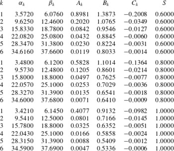
, making convergence reasonably achievable after only a few modes, as suggested by table 1, which gives the values of
 ${\it\beta}_{k}$
for
 $S=0.6$
, 0.8 and 1, for the first six modes. The stream function inside the channel is obtained by integrating expression (5.4) subject to
 ${\it\psi}_{2}(x\rightarrow -\infty ,z)=0$
, leading to
 $$\begin{eqnarray}{\it\psi}_{2}(x\leqslant 0,z)=\mathop{\sum }_{k=1}^{\infty }\frac{B_{k}}{{\it\beta}_{k}}\text{e}^{{\it\beta}_{k}x}V_{k}(z).\end{eqnarray}$$
The pressure inside the channel is determined by integrating equation (5.1b
) subject to the pressure condition at the wall, which is available upon setting
 $z=0$
in (5.1a
). In addition, since (4.10) suggests that
 $p_{2}(x=0,z=0)=0$
, then we obtain the desired boundary condition for pressure as
 $p_{2}(x\leqslant 0,z=0)=-4S\sum _{k=1}^{\infty }(B_{k}/{\it\beta}_{k})(\text{e}^{{\it\beta}_{k}x}-1)-8x$
. Inserting (5.6) into (5.1b
) and using (5.5) gives
 $$\begin{eqnarray}p_{2z}(x\leqslant 0,z)=u_{0}\mathop{\sum }_{k=1}^{\infty }{\it\beta}_{k}B_{k}\text{e}^{{\it\beta}_{k}x}V_{k}=-\mathop{\sum }_{k=1}^{\infty }\frac{B_{k}}{{\it\beta}_{k}}\text{e}^{{\it\beta}_{k}x}[(u_{0}V_{k}^{\prime })^{\prime }-(u_{0}^{\prime }V_{k})^{\prime }].\end{eqnarray}$$
Integrating subject to the pressure at the wall finally yields
 $$\begin{eqnarray}p_{2}(x\leqslant 0,z)=-8x-\mathop{\sum }_{k=1}^{\infty }\frac{B_{k}}{{\it\beta}_{k}}\{\text{e}^{{\it\beta}_{k}x}[u_{0}(z)V_{k}^{\prime }(z)-u_{0}^{\prime }(z)V_{k}(z)]-4S\}.\end{eqnarray}$$
Eigenvalues and expansion coefficients for different slip lengths,
 $S=0.6$
, 0.8 and 1.

To this order, the flow field inside the channel is given by
 $$\begin{eqnarray}\displaystyle & \displaystyle {\it\psi}(x\leqslant 0,z)={\it\psi}_{0}(z)+Re^{-1}\mathop{\sum }_{k=1}^{\infty }\frac{B_{k}}{{\it\beta}_{k}}\text{e}^{{\it\beta}_{k}x}V_{k}(z), & \displaystyle\end{eqnarray}$$
 $$\begin{eqnarray}\displaystyle & \displaystyle u(x\leqslant 0,z)=u_{0}(z)+Re^{-1}\mathop{\sum }_{k=1}^{\infty }\frac{B_{k}}{{\it\beta}_{k}}\text{e}^{{\it\beta}_{k}x}V_{k}^{\prime }(z), & \displaystyle\end{eqnarray}$$
 $$\begin{eqnarray}\displaystyle & \displaystyle w(x\leqslant 0,z)=-Re^{-1}\mathop{\sum }_{k=1}^{\infty }B_{k}\text{e}^{{\it\beta}_{k}x}V_{k}(z), & \displaystyle\end{eqnarray}$$
 $$\begin{eqnarray}\displaystyle & \displaystyle p(x\leqslant 0,z)=-Re^{-1}8x-Re^{-1}\mathop{\sum }_{k=1}^{\infty }\frac{B_{k}}{{\it\beta}_{k}}\{\text{e}^{{\it\beta}_{k}x}[u_{0}(z)V_{k}^{\prime }(z)-u_{0}^{\prime }(z)V_{k}(z)]-4S\}, & \displaystyle\end{eqnarray}$$
 $$\begin{eqnarray}\displaystyle & \displaystyle {\it\tau}_{xz}(x\leqslant 0,z)=u_{0}^{\prime }(z)-Re^{-1}\mathop{\sum }_{k=1}^{\infty }\frac{B_{k}}{{\it\beta}_{k}}\text{e}^{{\it\beta}_{k}x}\left(2{\it\beta}_{k}^{2}-\frac{u_{0}^{\prime \prime }}{u_{0}}\right)V_{k}(z), & \displaystyle\end{eqnarray}$$
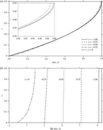
Upstream flow for
 $S=1$
at different positions: (a) velocity profiles at
 $Re=80$
, and (b) pressure profiles at any Reynolds number.

Although the coefficients
 $B_{k}$
will become available once the flow outside the channel is determined, it is helpful at this stage to nevertheless adopt their values from table 1 and examine the flow field as the fluid approaches the exit inside the channel. The upstream flow field is typically illustrated in figure 7 for
 $S=1$
, where the streamwise velocity and pressure profiles are depicted at various positions between
 $x=-1$
, where fully developed conditions are essentially met, and the channel exit is at
 $x=0$
. Figure 7(a) shows the velocity profiles for
 $Re=80$
, suggesting a rapid increase in slip as the fluid approaches
 $x=0$
. This is particularly clear from the inset. The difference between the wall and centreline velocities diminishes progressively, with gradual flattening of the velocity profile. Thus, as the fluid moves towards the channel exit, additional slippage occurs at the wall, and the flow decelerates in the core layer so as to satisfy the condition of continuity (see inset). This relative deceleration in the core layer is reduced for higher slip, and the flow retains increasingly its Poiseuille character. Figure 7(b) indicates, as expected, that the pressure profile at
 $x=-1$
presents no variation in the transverse direction. Closer to the channel exit, the pressure exhibits an almost antisymmetric variation: an increase in the pressure at the wall is accompanied by a decrease along the centreline.
Influence of slip and inertia on exit length
 $x_{0}$
(upstream position for fully developed flow): (a) exit length against
 $Re$
for different slip lengths, (b) exit length against
 $S$
for different Reynolds numbers.

Although Poiseuille conditions are theoretically recovered in the limit
 $x\rightarrow -\infty$
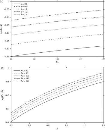
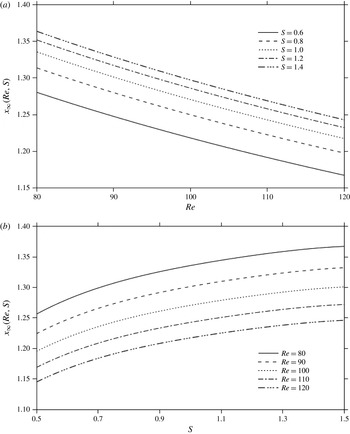
, calculations based on expressions (5.9), such as shown in figure 7 above, indicate that these conditions prevail essentially at a distance equal to one channel width. This is also the case in the absence of slip (Khayat Reference Khayat2014). As to the influence of slip, consider the exit length, the upstream position
 $x_{0}$
where fully developed Poiseuille flow is recovered inside the channel. Rather than seeking an accurate numerical prediction, an estimate of the influence of inertia and slip on the exit length is obtained analytically. Since the exit length is relatively large, only the contribution of the leading eigenmode is significant. In this case, by evaluating the relative departure in the velocity from (5.9b
) at the centreline, for relatively large distance, the exit length satisfies approximately:
 $(B_{1}/Re(4S+1){\it\beta}_{1})\text{e}^{{\it\beta}_{1}x_{0}}V_{1}^{\prime }(1/2)\simeq -10^{-c}$
, where
 $c$
is an imposed tolerance exponent. Thus,
 $$\begin{eqnarray}x_{0}(Re,S)=\frac{1}{{\it\beta}_{1}}\ln \left[-10^{-c}\frac{Re(4S+1){\it\beta}_{1}}{B_{1}}V_{1}^{\prime }\left(\frac{1}{2}\right)\right].\end{eqnarray}$$
Figure 8 depicts the influence of slip and inertia on the exit length for
 $c=4$
, which is plotted against
 $Re$
for different slip lengths (figure 8
a), and against
 $S$
for different Reynolds numbers (figure 8
b). The logarithmic dependence on
 $Re$
, which also corresponds to the behaviour predicted by Poole & Ridley (Reference Poole and Ridley2007) for the entry length in a duct at large Reynolds number (see their figure 2), is not entirely obvious from figure 8(a) over the
 $Re$
range in the figure. Figure 8 suggests that the exit length decreases both with inertia and, not surprisingly, with slip. In both cases, the viscous effect responsible for flow development is diminished; the Poiseuille character is retained up to a smaller upstream distance. In contrast, for a fluid entering a channel or a pipe, the entry length increases with slip (Chakraborty & Anand Reference Chakraborty and Anand2008; Duan & Muzychka Reference Duan and Muzychka2010). The two findings are not contradictory. For both entry and exit flows, slip (and inertia) helps retain upstream plug and parabolic flow conditions, respectively, over a longer distance.
Perhaps the most remarkable feature in figure 8 is the significant jump in exit length as
 $S$
increases, especially between adhering and slipping fluids (not shown). A similar phenomenon was also noted by Chakraborty & Anand (Reference Chakraborty and Anand2008) who examined the dependence of the entry length on the thickness of a thin gas layer at the wall. They observed that ‘even with a trace amount of nanobubble formation due to hydrophobic interactions, there is a rapid increment in the entrance length’. They also point out that a thickness (in unit of channel width) as small as
 $10^{-7}$
of the fluid layer can result in more than 50 % increase in the entry length, which was attributed to the presence of nanobubble layers covering the solid surface. Consequently, ‘the effect of wall shear penetrates into the bulk fluid only after the core flow has axially traversed a significantly greater distance than for the case devoid of any hydrophobic interactions’. The same mechanism also applies in the case of the jet exiting a hydrophobic channel, with the gas layer delaying the transition from Poiseuille conditions. In other words, and paraphrasing Chakraborty & Anand (Reference Chakraborty and Anand2008), the microscopic roughness of the solid surface impedes the motion of the fluid, ensuring adherence. In contrast, the gas layer acts as a shield, and prevents the liquid from direct contact with the surface irregularities and roughness.
5.2 Flow in the core layer outside the channel
At this stage, the solution process undergoes a major departure from the case of an adhering jet. Indeed, the flow outside the channel cannot be expressed in terms of the eigenfunctions
 $V_{k}$
as previously done (Tillett Reference Tillett1968; Khayat Reference Khayat2014). This is the result of the slip effect in the boundary condition for small
 $z$
in the jet region. This boundary condition is obtained by eliminating
 $h_{1}(x)$
between (4.6) and (4.7) to give
 $$\begin{eqnarray}{\it\psi}_{2}(x\geqslant 0,z=0)-S{\it\psi}_{2z}(x\geqslant 0,z=0)=2x.\end{eqnarray}$$
Consequently, in addition to matching with (5.4) at
 $x=0$
, the boundary conditions needed for the solution of (5.2) are
 $$\begin{eqnarray}w_{2}\left(x\geqslant 0,z={\textstyle \frac{1}{2}}\right)=0,\quad w_{2}(x\geqslant 0,z=0)-Sw_{2z}(x\geqslant 0,z=0)=-2.\end{eqnarray}$$
In this case, the solution takes the form
 $$\begin{eqnarray}w_{2}(x\geqslant 0,z)=-{\it\psi}_{2x}(x\geqslant 0,z)=-2U_{0}(z)+\mathop{\sum }_{k=1}^{\infty }A_{k}\text{e}^{-{\it\alpha}_{k}x}U_{k}(z),\end{eqnarray}$$
where
 $U_{0}(z)$
satisfies the following boundary-value problem:
 $$\begin{eqnarray}U_{0}^{\prime \prime }(z)-\frac{u_{0}^{\prime \prime }(z)}{u_{0}(z)}U_{0}(z)=0,\quad U_{0}(0)-SU_{0}^{\prime }(0)=1,\quad U_{0}\left(\frac{1}{2}\right)=0.\end{eqnarray}$$
Problem (5.14) possesses an analytical solution. The equation can be recast as
 $(U_{0}^{\prime }u_{0})^{\prime }-(U_{0}u_{0}^{\prime })^{\prime }=0,$
which, upon integrating, applying the mixed condition at
 $z=0$
and recalling (2.1), lead to
 $U_{0}^{\prime }u_{0}-U_{0}u_{0}^{\prime }=-4$
. Solving gives
 $$\begin{eqnarray}U_{0}(z)=\frac{S+z-z^{2}}{4S+1}\left[\frac{1-2z}{S+z-z^{2}}+\frac{4}{\sqrt{4S+1}}\tanh ^{-1}\left(\frac{1-2z}{\sqrt{4S+1}}\right)\right].\end{eqnarray}$$
Figure 9 illustrates the influence of slip on the
 $U_{0}$
profiles. The profiles also give the behaviour of the depthwise flow in the core region far from the exit, dominated by the first term in (5.13). In particular, the dependence of
 $U_{0}(0)$
on
 $S$
reflects the increasingly contracting jet as
 $S$
decreases. However, note that the behaviour of
 $w$
near the jet surface is fully established when the composite flow is determined (see § 6).
Influence of slip on
 $U_{0}(z)$
.

The functions
 $U_{k}\,(z)$
must satisfy the condition
 $U_{k}(0)-SU_{k}^{\prime }(0)=0$
. Without loss of generality, one then has the following eigenvalue problem:
 $$\begin{eqnarray}U_{k}^{\prime \prime }(z)+\left({\it\alpha}_{k}^{2}-\frac{u_{0}^{\prime \prime }(z)}{u_{0}(z)}\right)U_{k}(z)=0,\quad U_{k}(0)=S,\quad U_{k}^{\prime }(0)=1,\quad U_{k}\left(\frac{1}{2}\right)=0.\end{eqnarray}$$
Like
 $V_{k}$
, the
 $U_{k}$
eigenfunctions can be shown to be orthogonal (see appendix D). Note, however, that
 $V_{k}$
and
 $U_{k}$
are not mutually orthogonal. In fact, by adopting similar steps as in appendix B, it can be shown that
 $$\begin{eqnarray}\langle U_{j}V_{k}\rangle =\frac{S}{{\it\beta}_{k}^{2}-{\it\alpha}_{j}^{2}},\end{eqnarray}$$
where
 $\langle ~\rangle$
denotes integration over the interval
 $z\in [0,1/2]$
. Table 1 displays the dependence of
 ${\it\alpha}_{k}$
on
 $S$
for the first six eigenvalues.
The stream function is determined by integrating (5.13) subject to condition (5.11), suggesting that
 $$\begin{eqnarray}{\it\psi}_{2}(x\geqslant 0,z)=2U_{0}(z)x+\mathop{\sum }_{k=1}^{\infty }\left(\frac{A_{k}}{{\it\alpha}_{k}}\text{e}^{-{\it\alpha}_{k}x}+C_{k}\right)U_{k}(z),\end{eqnarray}$$
where the coefficients
 $C_{k}$
are determined by matching the flow at the channel exit (see below). Note that (5.18) also satisfies
 ${\it\psi}_{2}(x\geqslant 0,z=1/2)=0$
as (4.3) dictates.
The pressure outside the channel is obtained by first inserting
 ${\it\psi}_{2}(x\geqslant 0,z)$
from (5.18) into (5.1b
), and recalling (5.16) to yield
 $$\begin{eqnarray}p_{2z}(x\geqslant 0,z)=u_{0}\mathop{\sum }_{k=1}^{\infty }{\it\alpha}_{k}\text{e}^{-{\it\alpha}_{k}x}A_{k}U_{k}=-\mathop{\sum }_{k=1}^{\infty }\frac{A_{k}}{{\it\alpha}_{k}}\text{e}^{-{\it\alpha}_{k}x}[(U_{k}^{\prime }u_{0})^{\prime }-(U_{k}u_{0}^{\prime })^{\prime }].\end{eqnarray}$$
Integrating (5.19), subject to condition (4.10), and using the boundary conditions in (5.16), give
 $$\begin{eqnarray}p_{2}(x\geqslant 0,z)=-\mathop{\sum }_{k=1}^{\infty }\frac{A_{k}}{{\it\alpha}_{k}}\text{e}^{-{\it\alpha}_{k}x}[u_{0}(z)U_{k}^{\prime }(z)-u_{0}^{\prime }(z)U_{k}(z)].\end{eqnarray}$$
To this order, the flow outside the channel is summarized as
 $$\begin{eqnarray}\displaystyle & \displaystyle {\it\psi}(x\geqslant 0,z)={\it\psi}_{0}(z)+Re^{-1}\left[2U_{0}(z)x+\mathop{\sum }_{k=1}^{\infty }\left(\frac{A_{k}}{{\it\alpha}_{k}}\text{e}^{-{\it\alpha}_{k}x}+C_{k}\right)U_{k}(z)\right], & \displaystyle\end{eqnarray}$$
 $$\begin{eqnarray}\displaystyle & \displaystyle u(x\geqslant 0,z)=u_{0}(z)+Re^{-1}\left\{2U_{0}^{\prime }(z)x+\mathop{\sum }_{k=1}^{\infty }\left(\frac{A_{k}}{{\it\alpha}_{k}}\text{e}^{-{\it\alpha}_{k}x}+C_{k}\right)U_{k}^{\prime }(z)\right\}, & \displaystyle\end{eqnarray}$$
 $$\begin{eqnarray}\displaystyle & \displaystyle w(x\geqslant 0,z)=-Re^{-1}\left[2U_{0}(z)-\mathop{\sum }_{k=1}^{\infty }\text{e}^{-{\it\alpha}_{k}x}A_{k}U_{k}(z)\right], & \displaystyle\end{eqnarray}$$
 $$\begin{eqnarray}\displaystyle & \displaystyle p(x\geqslant 0,z)=-Re^{-1}\mathop{\sum }_{k=1}^{\infty }\frac{A_{k}}{{\it\alpha}_{k}}\text{e}^{-{\it\alpha}_{k}x}[u_{0}(z)U_{k}^{\prime }(z)-u_{0}^{\prime }(z)U_{k}(z)], & \displaystyle\end{eqnarray}$$
 $$\begin{eqnarray}\displaystyle & \displaystyle {\it\tau}_{xz}(x\geqslant 0,z)=u_{0}^{\prime }(z)+Re^{-1}\left\{2U_{0}^{\prime \prime }x+\mathop{\sum }_{k=1}^{\infty }\left[\left(\frac{A_{k}}{{\it\alpha}_{k}}\text{e}^{-{\it\alpha}_{k}x}+C_{k}\right)\frac{u_{0}^{\prime \prime }}{u_{0}}-C_{k}{\it\alpha}_{k}^{2}\right]U_{k}\right\}, & \displaystyle \nonumber\\ \displaystyle & & \displaystyle\end{eqnarray}$$
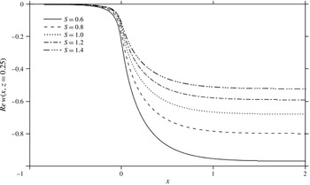
 $u$
experiences linear growth with downstream distance, coinciding with a levelling of
 $w(x,z)$
and vanishing of the pressure. Note that
 $w(x\geqslant 0,z)\sim -2Re^{-1}U_{0}(z)$
for large
 $x$
. At this stage, only the values of the expansion coefficients are missing, which we determine next.
5.3 Matching the flow at the channel exit
The coefficients,
 $A_{k},B_{k}$
and
 $C_{k}$
are now determined by matching the transverse velocity component, stream function and pressure at the channel exit. It is emphasized that although the flow is singular at the channel exit in the inner layer, it is continuous in the core region. Thus, upon evaluating
 $w(x,z)$
from (5.9c
) and (5.21c
) at
 $x=0$
, and matching, one obtains the following relation:
 $$\begin{eqnarray}2U_{0}(z)=\mathop{\sum }_{k=1}^{\infty }[B_{k}V_{k}(z)+A_{k}U_{k}(z)].\end{eqnarray}$$
This relation is a spectral representation of
 $U_{0}\,(z)$
in terms of the orthogonal functions
 $V_{k}\,(z)$
and
 $U_{k}\,(z)$
. Matching the pressure from (5.9d
) and (5.21d
) gives
 $$\begin{eqnarray}\mathop{\sum }_{k=1}^{\infty }\left\{\frac{B_{k}}{{\it\beta}_{k}}[u_{0}(z)V_{k}^{\prime }(z)-u_{0}^{\prime }(z)V_{k}(z)-4S]-\frac{A_{k}}{{\it\alpha}_{k}}[u_{0}(z)U_{k}^{\prime }(z)-u_{0}^{\prime }(z)U_{k}(z)]\right\}=0.\end{eqnarray}$$
A more suitable relation is obtained upon differentiating (5.23) and using the equations in (5.5) and (5.16), namely
 $$\begin{eqnarray}\mathop{\sum }_{k=1}^{\infty }[{\it\beta}_{k}B_{k}V_{k}(z)-{\it\alpha}_{k}A_{k}U_{k}(z)]=0.\end{eqnarray}$$
Note that this relation ensures the marching of the shear stress. Projecting both (5.22) and (5.24) onto
 $V_{k}\,(z)$
, and using (5.17), allow the expression of
 $B_{k}$
in terms of
 $A_{k}$
as
 $$\begin{eqnarray}B_{k}=\frac{S}{{\it\beta}_{k}\langle V_{k}V_{k}\rangle }\mathop{\sum }_{j=1}^{\infty }\frac{{\it\alpha}_{j}A_{j}}{{\it\beta}_{k}^{2}-{\it\alpha}_{j}^{2}},\end{eqnarray}$$
and the evaluation of the coefficients
 $A_{k}$
through the system of equations
 $$\begin{eqnarray}\mathop{\sum }_{j=1}^{\infty }\frac{A_{j}}{{\it\beta}_{k}-{\it\alpha}_{j}}=\frac{2}{S}{\it\beta}_{k}\langle V_{0}V_{k}\rangle .\end{eqnarray}$$
Finally, the third relation ensues from evaluating the stream functions in (5.9a
) and (5.21a
) at
 $x=0$
, and comparing:
 $$\begin{eqnarray}\mathop{\sum }_{k=1}^{\infty }\frac{B_{k}}{{\it\beta}_{k}}V_{k}(z)=\mathop{\sum }_{k=1}^{\infty }\left(\frac{A_{k}}{{\it\alpha}_{k}}+C_{k}\right)U_{k}(z).\end{eqnarray}$$
Upon projection and use of relations (5.17), (5.22) and (5.24), we obtain the following set of equations for
 $C_{k}$
:
 $$\begin{eqnarray}{\it\beta}_{k}\mathop{\sum }_{j=1}^{\infty }\left(\frac{C_{j}}{{\it\beta}_{k}^{2}-{\it\alpha}_{j}^{2}}\right)=\frac{2}{S}\left\langle V_{0}V_{k}\right\rangle -\mathop{\sum }_{j=1}^{\infty }\frac{A_{j}}{{\it\alpha}_{j}}\left(\frac{1}{{\it\beta}_{k}-{\it\alpha}_{j}}\right).\end{eqnarray}$$
Now that the coefficients have been determined, the flow field becomes available at any position in the core region, inside and outside the channel. Incidentally, expressions (5.9d
) and (5.21d
) are valid throughout the entire flow region as
 ${\it\varepsilon}^{2}p_{2}(x,z)$
turns out to be equal to the composite pressure (see § 6). In other words, the pressure is everywhere readily available and is given by
 $p(x,z)={\it\varepsilon}^{2}p_{2}(x,z)+O({\it\varepsilon}^{3})$
.
5.4 Influence of slip on the flow in the core layer and jet profile
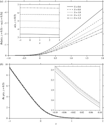
Influence of slip on flow along centreline: (a) deviation of streamwise from Poiseuille level. Inset shows actual streamwise velocity component at
 $Re=80$
, and (b) pressure, for different slip parameters. Inset shows magnification of pressure curves.

The character of the flow in the core region is reflected in the behaviour of velocity and pressure along the centreline. Figure 10 depicts the influence of slip on the streamwise velocity component
 $u(x,z=1/2)$
, and pressure
 $Re\,p(x,z=1/2)$
at any Reynolds number inside and outside the channel as functions of
 $x$
. Figure 10(a) shows the deviation from the Poiseuille level for each
 $S$
. The streamwise flow (inset in figure 10
a) retains its Poiseuille level,
 $4S$
 $+$
1, up to an upstream distance from the channel exit that decreases with slip (see figure 8). At that point
 $u$
decreases as a result of flow weakening downstream for any slip level, accompanied by the vanishing of the pressure (figure 10
b). There is an essentially linear growth in velocity departure, reflected in the
 $U_{0}^{\prime }(z)x$
term in (5.21b
), which weakens the flow and eventually halts it, as illustrated in the
 $S=0$
profile. However, at this point, the current formulation ceases to be valid. In reality, the velocity begins to flatten as the jet approaches uniform flow conditions (see Philippe & Dumargue Reference Philippe and Dumargue1991). The slope of the velocity at the centreline far downstream is determined from (5.21b
) at
 $z=1/2$
. In addition, recalling that
 $U_{0}^{\prime }(z)u_{0}(z)-U_{0}(z)u_{0}^{\prime }(z)=-4$
, then we have
 $$\begin{eqnarray}u_{x}\left(x\geqslant 0,\frac{1}{2}\right)=2Re^{-1}U_{0}^{\prime }\left(\frac{1}{2}\right)=-\frac{2}{(4S+1)Re}.\end{eqnarray}$$
In the presence of strong slip, inertia remains dominant, with the flow retaining its Poiseuille character over longer distance, which is also reflected in the larger (streamwise) pressure gradient (see the case for
 $S=1$
, for instance). Note that the upstream pressure gradient is the same for any slip level. A slipping jet experiences a milder departure from the Poiseuille level in velocity and pressure. In particular, for
 $S=1$
, figure 10 suggests that Poiseuille flow is essentially prevalent everywhere inside and, to a lesser extent, outside the channel; the pressure gradient remains constant for a relatively large downstream distance from the channel exit, at which point the pressure levels off and vanishes. For smaller
 $S$
, the contraction is relatively significant, resulting in stronger streamwise flow as figure 10 indicates. In this case, inertia becomes essentially the only driving force to balance viscous force as the jet exits the channel, without any driving pressure. In contrast, a slipping jet experiences less friction, which relatively enhances the effect of inertia. Consequently, the jet behaves closer to inviscid than viscous flow, with inertia being predominantly balanced by a driving pressure. In fact, figure 10 suggests that for large
 $S$
, the driving pressure force remains essentially the same as for Poiseuille flow However, there is a saturation behaviour as
 $S$
increases, and we may not be able to infer the large
 $S$
behaviour given that
 $S=O(1)$
in the present formulation. In general, the more slipping fluid tends to retain further (and farther) its original (upstream) Poiseuille character in pressure and velocity, with reduced contraction.
The change of
 $u$
along the centreline reflects the presence of normal (elongational) stress, and is, evidently, accompanied by a change in
 $w$
in the transverse direction, starting from the zero level at the centreline. Figure 11 displays the influence of slip on the transverse flow at
 $z=0.25$
. The effect of flow discontinuity remains felt at this height, but lessens with slip. Far from the exit,
 $w$
tends to level off at a value equal to
 $-\!2Re^{-1}U_{0}(0.25;S)$
. This value increases with
 $S$
(see figure 10
a). Figure 11 shows that
 $w$
is negative, as expected, since
 $w_{z}(x,z=1/2)=-u_{x}(x,z=1/2)>0$
, suggesting a fountain flow character of the jet in the core layer, which does not prevail necessarily over the entire (half) width of the jet unless the jet is expanding (see below).
Influence of slip on transverse velocity profiles in the core layer
 $(x=0.25)$
.

Influence of slip and inertia on relaxation length
 $x_{\infty }$
: (a) relaxation length against
 $Re$
for different slip lengths, (b) relaxation length against
 $S$
for different Reynolds numbers.

We consider next the relaxation length
 $x_{\infty }$
or the downstream distance from the channel exit where the pressure gradient vanishes as suggested by figure 10(b). Like the exit length, an estimate of the influence of inertia and slip on the relaxation lengths is obtained analytically, accounting only for the contribution of the leading eigenmode. In this case, evaluating the pressure gradient from (5.21d
) at the centreline, the relaxation length becomes
 $$\begin{eqnarray}x_{\infty }(Re,S)=-\frac{1}{{\it\alpha}_{1}}\ln \left[-\frac{10^{-c}Re}{(4S+1)A_{1}U_{1}^{\prime }\left({\textstyle \frac{1}{2}}\right)}\right].\end{eqnarray}$$
The resulting profiles are displayed in figure 12 for
 $c=3$
against the Reynolds number, and should be contrasted with those reported earlier in figure 8 for the exit length. The relaxation length increases with
 $S$
but decreases with
 $Re$
. Interestingly, in comparison to an adhering jet, a slipping jet tends to recover more rapidly its Poiseuille profile upstream but takes longer to relax downstream from the channel exit. In general,
 $x_{\infty }(S>0)>-x_{0}(S<0)$
.
Finally, the jet profile is now determined by evaluating
 ${\it\psi}_{2}(x,z)$
from (5.18) at
 $z=0$
, and substituting into (4.6). We obtain
 $h_{1}(x)$
, and, consequently, the jet height as
 $$\begin{eqnarray}{\it\zeta}(x;Re,S)=\frac{Re^{-1}}{4S}\left\{\left[\frac{1}{S}-2U_{0}(0;S)\right]x-S\mathop{\sum }_{k=1}^{\infty }\left(\frac{A_{k}}{{\it\alpha}_{k}}\text{e}^{-{\it\alpha}_{k}x}+C_{k}\right)\right\},\end{eqnarray}$$
where (5.15) is evaluated at
 $z=0$
to give
 $$\begin{eqnarray}U_{0}(0;S)=\frac{S}{4S+1}\left[\frac{1}{S}+\frac{4}{\sqrt{4S+1}}\tanh ^{-1}\left(\frac{1}{\sqrt{4S+1}}\right)\right].\end{eqnarray}$$
At the channel exit,
 $$\begin{eqnarray}{\it\zeta}(x=0;Re,S)=-\frac{Re^{-1}}{4}\mathop{\sum }_{k=1}^{\infty }\left(\frac{A_{k}}{{\it\alpha}_{k}}+C_{k}\right)=0,\end{eqnarray}$$
which follows from evaluating (5.18) at
 $z=0$
and using the boundary conditions in (5.5) and (5.16). Thus, the jet height vanishes at the channel exit. Figure 13 illustrates the influence of slip on the jet profile for any Reynolds number. As expected, the jet height decreases with increasing slip effect. The jet height grows monotonically with distance. Like an adhering jet (Tillett Reference Tillett1968; Khayat Reference Khayat2014), a slipping jet contracts indefinitely (until uniform conditions are reached far downstream). This was predicted and verified experimentally by Philippe & Dumargue (Reference Philippe and Dumargue1991) for an adhering jet. Expression (5.31) indicates that the jet behaves linearly close to the exit as well as far from the exit; with a decrease in slope equal to
 $(Re^{-1}/4)\sum _{k=1}^{\infty }A_{k}$
. Consequently, more inertial jets tend to be flatter.
Jet profiles for different slip parameter values.

6 Flow over the entire jet region
 $(x>0)$

The flow at any location in the jet region (outside the channel) is obtained by determining the composite velocity and pressure. Following Van Dyke (Reference Van Dyke1975), the composite-expansion operations are defined by
 $$\begin{eqnarray}C_{i}{\it\psi}\equiv E_{i}{\it\psi}+H_{i}{\it\psi}-E_{i}H_{i}{\it\psi},\quad C_{i}p\equiv E_{i}p+H_{i}p-E_{i}H_{i}p.\end{eqnarray}$$
This expression provides a uniform approximation to order
 ${\it\varepsilon}^{i}$
over the whole width of the jet. Given the availability of the treatment in the previous section, it is convenient to first generate
 $C_{2}{\it\psi}$
, and then deduce
 $C_{1}u$
and
 $C_{2}w$
. The composite stream function is constructed by invoking the expressions of
 $H_{2}{\it\psi}$
and
 $E_{2}{\it\psi}$
(see appendix C):
 $$\begin{eqnarray}\displaystyle & \displaystyle H_{2}{\it\psi}=4S{\it\varepsilon}{\it\eta}+{\it\varepsilon}^{2}{\it\xi}f_{2}=4Sy+{\it\varepsilon}^{2}{\it\xi}f_{2}, & \displaystyle\end{eqnarray}$$
 $$\begin{eqnarray}\displaystyle & \displaystyle E_{2}{\it\psi}=4S(y+{\it\varepsilon}^{2}h_{1})+2(y^{2}+2y{\it\varepsilon}^{2}h_{1})-{\textstyle \frac{4}{3}}(y^{3}+3y^{2}{\it\varepsilon}^{2}h_{1})+{\it\varepsilon}^{2}{\it\psi}_{2}(x,z). & \displaystyle\end{eqnarray}$$
In this case,
 $$\begin{eqnarray}H_{2}E_{2}{\it\psi}=4S(y+{\it\varepsilon}^{2}h_{1})+2y^{2}+{\it\varepsilon}^{2}{\it\psi}_{2}(x,0),\end{eqnarray}$$
and the composite stream function is given by
 $$\begin{eqnarray}C_{2}{\it\psi}(x,z)=4Sz-\frac{4}{3}z^{3}+Re^{-1}\left[xf_{2}({\it\theta})+4zh_{1}(x)+{\it\psi}_{2}(x\geqslant 0,z)-\frac{x}{S}\right]+O(Re^{-3/2}).\end{eqnarray}$$
As a check on the validity of this composite expression, there are three limits that it must satisfy. The first limit is at the channel exit and large
 ${\it\theta}$
where (6.5) must collapse onto (5.21a
). Indeed, noting that
 ${\it\varepsilon}^{2}{\it\xi}f_{2}({\it\theta})\rightarrow 2(z^{2}-2z{\it\varepsilon}^{2}h_{1})+{\it\varepsilon}^{2}(x/S)$
for large
 ${\it\theta}$
, then (6.5) reduces to
 $C_{2}{\it\psi}(x=0,z)={\it\psi}_{0}(z)+{\it\varepsilon}^{2}{\it\psi}_{2}(x=0,z)$
. The second limit is at the jet surface. In this case, setting
 $z={\it\zeta}={\it\varepsilon}^{2}h_{1}$
in (6.5), we find that
 $C_{2}{\it\psi}(x,{\it\zeta})={\it\varepsilon}^{2}xf_{2}(0)$
, which agrees with (3.19) for
 ${\it\eta}=0$
. Finally, the third limit is at the jet centreline. Setting
 $z=1/2$
in (6.5) and assuming large
 ${\it\theta}$
, we have
 $C_{2}{\it\psi}(x,z=1/2)={\it\psi}_{0}(z=1/2)$
.
Similarly, the composite streamwise and transverse velocity components are written down to first and second order, respectively, as
 $$\begin{eqnarray}\displaystyle C_{1}u(x,z)=4S-4z^{2}+\sqrt{\frac{x}{Re}}f_{2}^{\prime }({\it\theta})+O(Re^{-1}), & & \displaystyle\end{eqnarray}$$
 $$\begin{eqnarray}\displaystyle C_{2}w(x,z)=Re^{-1}\left\{w_{2}(x,z)+\frac{1}{4S}[4-f_{2}^{\prime \prime }({\it\theta})]\right\}+O(Re^{-3/2}). & & \displaystyle\end{eqnarray}$$
Here
 ${\it\psi}_{2},u_{2}$
and
 $w_{2}$
are given through (5.18), and its derivatives. Finally, the pressure is readily available to
 $O({\it\varepsilon}^{2})$
, or
 $$\begin{eqnarray}C_{2}p(x,z)=Re^{-1}p_{2}(x\geqslant 0,z)+O(Re^{-3/2}),\end{eqnarray}$$
where
 $p_{2}$
is given by (5.20).
Figure 14 depicts the streamwise flow component for
 $S=0.6$
. The figure shows the velocity profiles at different downstream positions, including the exit (
 $x=0$
). The height of the inner layer,
 $z={\it\zeta}(x)+{\it\delta}(x)$
is also displayed as well as that of the jet surface,
 $z={\it\zeta}(x)$
. For any slip length, the flow retains essentially its Poiseuille character of figure 2 at the exit, despite the presence of a significant vertical flow component as reflected by (6.7). Further downstream, there is growing slip at the free surface, with the flow becoming increasingly uniform with transverse position. The flow becomes predominantly elongational, with sustained normal stress effect. That shearing weakens with distance is evident from the profile flattening as well as from the increase in velocity at the surface relative to the velocity along the centreline. Simultaneously, the inner-layer region thickens at a higher rate for the less slipping fluid. Its consequence is particularly felt by the flow in the transverse direction as discussed next.
Composite streamwise velocity profiles at different positions in the jet region for
 $S=0.6$
. Here
 $Re=100$
. Jet surface (dashed line) and inner-layer height (dotted lines) also shown. Vertical lines indicate
 $x$
position.

Composite transverse velocity profiles at different positions in the jet region for
 $S=0.6$
. Note that
 $x$
positions are the same as in figure 14.

The corresponding transverse velocity profiles are depicted in figure 15 at the same positions. Generally, the velocity is positive near the jet surface as a result of jet contraction; recall from figure 4(a) that the streamwise velocity component is always positive. At some height, which increases slightly with slip,
 $w$
becomes and remains negative until it vanishes at the centreline, exhibiting essentially a linear growth with respect to
 $z$
before and after the turning point. Shearing and elongation are particularly strong near the exit as a result of the sharp jump in depthwise motion at
 $x=0$
, especially for a jet with low slip. For a slipping jet, the contraction weakens, and so does the depthwise motion. Generally,
 $w$
diminishes in intensity with distance from the channel exit, to become uniform at a rate that increases with slip. It is important to observe the progressive drop in accuracy as the boundary layer grows, particularly for the smaller
 $S$
cases (not shown). Recall from (3.25) that the boundary layer grows predominantly like
 ${\it\delta}\approx \sqrt{x/S\,Re}$
. Consequently, the lower the slip (and/or inertia), the faster the growth. However, if
 ${\it\delta}$
is large compared to the jet width, the current formulation ceases to be valid, as the inner solution dictates the flow field. This becomes particularly clear for small
 $S$
, where
 $w$
does not vanish at the centreline, reflecting the invalidity of the present formulation for small
 $S$
.
7 Influence of slip on jet thickness and speed far from channel exit
In this section, the flow is examined far downstream from the channel exit by adopting an integral approach. From conservation of mass and linear momentum,
 $$\begin{eqnarray}\int _{C}\boldsymbol{u}\boldsymbol{\cdot }\boldsymbol{n}\,\text{d}l=0,\quad \int _{C}({\bf\sigma}-\boldsymbol{u}\boldsymbol{u})\boldsymbol{\cdot }\boldsymbol{n}\,\text{d}l=0\end{eqnarray}$$
where
 $\boldsymbol{u}$
is the velocity vector and
 ${\bf\sigma}$
is the total stress tensor, which is scaled similarly to the pressure (see § 2). Thus:
 $$\begin{eqnarray}{\bf\sigma}=-p\unicode[STIX]{x1D644}+Re^{-1}(\boldsymbol{{\rm\nabla}}\boldsymbol{u}+\boldsymbol{{\rm\nabla}}\boldsymbol{u}^{t}).\end{eqnarray}$$
Here
 $\unicode[STIX]{x1D644}$
is the identity tensor,
 $\text{d}l$
denotes a line element of the closed curve
 $C$
and
 $\boldsymbol{n}$
is the unit normal vector outward at
 $C$
. The curve
 $C$
consists of the following arcs illustrated in figure 1: (i) a line
 $x=x_{0}<0$
,
 $0\leqslant z\leqslant 1/2$
far upstream, (ii) a segment
 $x_{0}\leqslant x\leqslant 0$
,
 $z=0$
along the (lower) wall, (iii) a segment
 $0\leqslant x\leqslant x_{\infty }$
,
 $z={\it\zeta}\,(x)$
of the lower free streamline, (iv) a line
 $x=x_{\infty }$
,
 ${\it\zeta}\,(x_{\infty })\leqslant z\leqslant 1/2$
downstream and (v) the segment
 $x_{0}\leqslant x\leqslant x_{\infty }$
,
 $z=1/2$
along the symmetry line.
More explicitly, the stress components are given by
 $$\begin{eqnarray}{\it\sigma}_{xx}=-p+2{\it\varepsilon}^{2}u_{x},\quad {\it\sigma}_{xz}={\it\sigma}_{zx}={\it\varepsilon}^{2}(u_{z}+w_{x}),\quad {\it\sigma}_{zz}=-p-2{\it\varepsilon}^{2}u_{z}.\end{eqnarray}$$
Only the
 $x$
component of (7.1) is considered. Thus, since there is no traction on the free surface, (iii) will not make any contribution. Also, from symmetry, there is no contribution along (v). For large
 $x_{\infty }$
, one obtains:
 $$\begin{eqnarray}\int _{0}^{1/2}[p-2{\it\varepsilon}^{2}u_{x}+u^{2}]_{x=x_{0}}\,\text{d}z-{\it\varepsilon}^{2}\int _{x_{0}}^{0}u_{z}(x,0)\,\text{d}x-\int _{{\it\zeta}(x_{\infty })}^{1/2}[p-2{\it\varepsilon}^{2}u_{x}+u^{2}]_{x=x_{\infty }}\,\text{d}z=0.\end{eqnarray}$$
Obviously, only contributions to
 $O({\it\varepsilon}^{2})$
will be considered. Consider the first and second integrals. Far upstream, the flow is fully developed, with no inner layer. In this case, for large
 $|x_{0}|$
, one deduces
 $u(x_{0},z)\sim u_{0}(z)$
from (5.9b
), and
 $p(x_{0},z)\sim -8{\it\varepsilon}^{2}x_{0}$
from (5.9d
), so that the first integral reads
 $$\begin{eqnarray}\int _{0}^{1/2}[p-2{\it\varepsilon}^{2}u_{x}+u^{2}]_{x=x_{0}}\,\text{d}z=-4{\it\varepsilon}^{2}x_{0}+\frac{4}{15}+\frac{8}{3}S+8S^{2}.\end{eqnarray}$$
Upon recalling from (5.9b
) that
 $u_{z}(x\leqslant 0,z=0)=u_{0}^{\prime }(0)+{\it\varepsilon}^{2}\sum _{k=1}^{\infty }(B_{k}/{\it\beta}_{k})\text{e}^{{\it\beta}_{k}x}V_{k}^{\prime \prime }(0)=4$
, the second integral reduces to
 $$\begin{eqnarray}{\it\varepsilon}^{2}\int _{x_{0}}^{0}u_{z}(x,0)\,\text{d}x=-4{\it\varepsilon}^{2}x_{0}.\end{eqnarray}$$
Substituting (7.5) and (7.6) into (7.4), and noting the uniform flow conditions far downstream, the momentum integral relation reduces to
 $$\begin{eqnarray}{\textstyle \frac{1}{2}}U^{2}T={\textstyle \frac{4}{15}}+{\textstyle \frac{8}{3}}S+8S^{2}.\end{eqnarray}$$
Here
 $T$
and
 $U$
are the constant (dimensionless) thickness and speed of the uniform jet. From mass conservation,
 $$\begin{eqnarray}\frac{1}{2}UT=\int _{0}^{1/2}u_{0}\,\text{d}z=\frac{1}{3}+2S=\frac{1+6S}{3}.\end{eqnarray}$$
Finally, the contraction ratio and jet velocity become
 $$\begin{eqnarray}T(S)=\frac{5}{6}\frac{(1+6S)^{2}}{1+10S+30S^{2}},\quad U(S)=\frac{4}{5}\frac{1+10S+30S^{2}}{1+6S}.\end{eqnarray}$$
In the limit of a sticking jet,
 $T(S=0)=5/6$
and
 $U(S=0)=4/5$
, which agrees with Tillett (Reference Tillett1968) and Khayat (Reference Khayat2014) for a Newtonian jet. Interestingly, for large
 $S$
,
 $T=1$
and
 $U=4S=u_{0}(z=1/2)$
, indicating that the jet preserves its width and speed, as in the case of an extremely shear-thinning jet (Khayat Reference Khayat2014). Figure 16 depicts the influence of slip on
 $U$
and
 $T$
. While the growth of the velocity ratio is essentially linear with slip length, the jet width ratio grows rapidly for small
 $S$
but eventually saturates asymptotically towards
 $T=1$
for large
 $S$
. The rapid growth and saturation phenomena are commensurate with the earlier findings throughout this study (see next section).
Influence of slip on jet thickness,
 $T$
, and speed,
 $U$
, ratios (relative to channel exit) for the jet far downstream.

8 Concluding remarks
The paper deals with a moderate Reynolds number liquid stream emerging from a 2-D channel to form a free-surface jet. The fluid is assumed to experience partial slip at the channel walls. The interplay between inertia and slip is emphasized. The problem is treated by the method of singular matched asymptotic expansions. At the exit of the jet a singularity occurs where the boundary condition changes from partial slip at the channel wall to tension free on the free surface of the jet. Surface tension effect is neglected. The flow domain thus consists of two different layers, namely an inner layer, adjacent to the unknown free surface of the jet, and a rotational inviscid core adjoining the centreline (see figure 1). The slip is assumed to be relatively large, with ratio,
 $S$
, of slip length to channel width of order one. The flow is matched at successive orders in the small parameter
 ${\it\varepsilon}$
, which is identified as the inverse of a suitable power of the Reynolds number. The relation between
 ${\it\varepsilon}$
and
 $Re$
is determined by ensuring the balance of inertial and viscous terms in the momentum conservation equation, and identifying the order of the leading term in the inner layer. In the presence of slip, it is established that
 ${\it\psi}=O({\it\varepsilon})$
and
 ${\it\varepsilon}=Re^{-1/2}$
as opposed to
 ${\it\psi}=O({\it\varepsilon}^{2})$
and
 ${\it\varepsilon}=Re^{-1/3}$
for an adhering jet.
In contrast to an adhering jet, it is possible to determine analytically the similarity solution to each order considered (see § 3.1). This is possible when the slip length is relatively large, which is a fundamental assumption in the present paper. Generally, the similarity form of the solution found in the inner layer allows us to avoid dealing explicitly with the singularity at the exit point, and does not require matching with the corresponding layer inside the channel. Instead the rotational, inviscid core layer has to be matched at the exit section where the core solution changes from the fully developed profile well inside the channel to the profile at the exit of the channel. The composite flow in the entire jet domain is obtained after matching the flows between the inner and outer layers.
In comparison to an adhering jet, the presence of slip adds a significant challenge in the matching process, both at the channel exit
 $(x=0)$
and at the inner–outer-layer interface. For an adhering jet, be it Newtonian (Tillett Reference Tillett1968; Miyake et al.
Reference Miyake, Yukai and Iemoto1979; Philippe & Dumargue Reference Philippe and Dumargue1991) or non-Newtonian (Saffari & Khayat Reference Saffari and Khayat2009; Khayat Reference Khayat2014), the core solutions inside and outside the channel are obtained in terms of the same spectral representation, in terms of orthogonal functions,
 $V_{k}\,(z)$
, resulting in the same eigenvalue problem inside and outside the channel. In contrast, for a slipping jet, different eigenmodes,
 $U_{k}\,(z)$
, are required for the flow outside the channel. The choice of the eigenfunctions
 $U_{k}\,(z)$
is not obvious since a mixed boundary condition, (5.11), involving slip effect, must be satisfied. Note that this condition reduces to a Dirichlet condition for
 $S=0$
, which is much less difficult to handle. The flow field must also match at the channel exit in the core layer. Given the inviscid rotational character of the core layer, the problem reduces to determining the transverse velocity component, and matching it at the channel exit. For an adhering jet, the remaining flow field (stream function and pressure) matches readily. In contrast, for a slipping jet, the matching of every field quantity, including the stream function, pressure and stress, must be ensured, leading to additional coupled relations, such as (5.22)–(5.24) and (5.27), which govern additional expansion coefficients.
Although an adhering jet is found to contract more than a slipping jet, the contraction is not necessarily accompanied by an increase in streamwise flow along the jet surface because of higher viscous dissipation. In fact, figure 4 shows little influence of slip on the velocity relative to the slip flow velocity at the wall. Thus, slip plays a role similar to inertia, prohibiting jet contraction. The inner-layer thickness is
 $O(Re^{-1/2})$
and decreases with slip length like
 $S^{-1/2}$
. The free-surface height is
 $O(Re^{-1})$
for a slipping jet, compared to
 $O(Re^{-1/3})$
for an adhering jet. Moreover, an adhering jet contracts with downstream distance like
 $x^{1/3}$
, whereas a slipping jet does not obey a clear behaviour except near and far from the channel exit where it contracts linearly with
 $x$
. Eventually, the jet reaches uniform conditions far downstream.
The developing upstream distance (exit length) inside the channel, and the relaxation downstream distance for the jet, are found to grow logarithmically with the Reynolds number, as in the case of entry flow (Poole & Ridley Reference Poole and Ridley2007). A slipping jet exhibits a shorter exit length and a longer relaxation length. Hence, a slipping jet tends to lose its Poiseuille character at a position closer to the channel exit, and relaxes to uniform jet conditions over a longer distance compared to an adhering jet. An integral approach is also implemented, suggesting that the jet contracts with a ratio (relative to channel width) of
 $(5/6)((1+6S)^{2}/(1+10S+30S^{2}))$
far downstream, at a relative speed of
 $(4/5)((1+10S+30S^{2})/(1+6S))$
. Note that the limits,
 $5/6$
and
 $4/5$
, corresponding to an adhering jet
 $(S=0)$
, are recovered (Tillett Reference Tillett1968). As in the case of entry flow (Chakraborty & Anand Reference Chakraborty and Anand2008; Duan & Muzychka Reference Duan and Muzychka2010), there is a rapid departure in flow behaviour for a slipping jet from the
 $S=0$
limit. This rapid change is notably observed in the drop of boundary-layer thickness, increase in exit and relaxation lengths as well as in jet width with slip length.
Finally, the solution procedure developed here, as in previous studies, is important since the singularity at the exit makes a converged purely numerical solution difficult to achieve. It can be used, e.g. as initial condition a little downstream the exit for a purely numerical solution, as is done in problems of transition to turbulence in the classical Blasius boundary-layer flow.
Acknowledgements
The author acknowledges the financial support of the Natural Science and Engineering Research Council of Canada.
Appendix A. Transformed equations and boundary conditions in the inner layer
Upon applying transformation (3.1), and recalling that
 $Re={\it\varepsilon}^{-1/{\it\alpha}}$
, (2.3) can be rewritten as
 $$\begin{eqnarray}\displaystyle {\it\psi}_{{\it\eta}}{\it\psi}_{{\it\xi}{\it\eta}}-{\it\psi}_{{\it\xi}}{\it\psi}_{{\it\eta}{\it\eta}} & = & \displaystyle -{\it\varepsilon}({\it\varepsilon}p_{{\it\xi}}-h^{\prime }p_{{\it\eta}})+{\it\varepsilon}^{(1/{\it\alpha}-1)}{\it\psi}_{{\it\eta}{\it\eta}{\it\eta}}\nonumber\\ \displaystyle & & \displaystyle +\,{\it\varepsilon}^{(1/{\it\alpha}+1)}({\it\psi}_{{\it\xi}{\it\xi}{\it\eta}}-h^{\prime \prime }{\it\psi}_{{\it\eta}{\it\eta}}-2h^{\prime }{\it\psi}_{{\it\xi}{\it\eta}{\it\eta}}+h^{\prime 2}{\it\psi}_{{\it\eta}{\it\eta}{\it\eta}}),\end{eqnarray}$$
 $$\begin{eqnarray}\displaystyle & & \displaystyle -{\it\psi}_{{\it\eta}}{\it\psi}_{{\it\xi}{\it\xi}}+{\it\psi}_{{\it\xi}}{\it\psi}_{{\it\xi}{\it\eta}}+h^{\prime \prime }{\it\psi}_{{\it\eta}}^{2}+h^{\prime }({\it\psi}_{{\it\eta}}{\it\psi}_{{\it\xi}{\it\eta}}-{\it\psi}_{{\it\xi}}{\it\psi}_{{\it\eta}{\it\eta}})\nonumber\\ \displaystyle & & \displaystyle \qquad =-p_{{\it\eta}}-{\it\varepsilon}^{(1/{\it\alpha}-1)}({\it\psi}_{{\it\xi}{\it\eta}{\it\eta}}-h^{\prime }{\it\psi}_{{\it\eta}{\it\eta}{\it\eta}})-{\it\varepsilon}^{(1/{\it\alpha}+1)}\left(\frac{\partial }{\partial {\it\xi}}-h^{\prime }\frac{\partial }{\partial {\it\eta}}\right)^{3}{\it\psi}.\end{eqnarray}$$
Similarly, the boundary conditions (2.4) become
 $$\begin{eqnarray}\displaystyle & \displaystyle {\it\psi}({\it\xi},{\it\eta}=0)=0, & \displaystyle\end{eqnarray}$$
 $$\begin{eqnarray}\displaystyle & \displaystyle h^{\prime }p({\it\xi},{\it\eta}=0)-{\it\varepsilon}^{1/{\it\alpha}-1}\left[\left(\frac{\partial }{\partial {\it\xi}}-h^{\prime }\frac{\partial }{\partial {\it\eta}}\right)^{2}{\it\psi}+2h^{\prime }({\it\psi}_{{\it\xi}{\it\eta}}-h^{\prime }{\it\psi}_{{\it\eta}{\it\eta}})-{\it\varepsilon}^{-2}{\it\psi}_{{\it\eta}{\it\eta}}\right]_{{\it\xi},{\it\eta}=0}=0, & \displaystyle \nonumber\\ \displaystyle & & \displaystyle\end{eqnarray}$$
 $$\begin{eqnarray}\displaystyle & \displaystyle p({\it\xi},{\it\eta}=0)+{\it\varepsilon}^{1/{\it\alpha}-1}\left[2{\it\psi}_{{\it\xi}{\it\eta}}-h^{\prime }{\it\psi}_{{\it\eta}{\it\eta}}-{\it\varepsilon}^{2}h^{\prime }\left(\frac{\partial }{\partial {\it\xi}}-h^{\prime }\frac{\partial }{\partial {\it\eta}}\right)^{2}{\it\psi}\right]_{{\it\xi},{\it\eta}=0}=0. & \displaystyle\end{eqnarray}$$
 $$\begin{eqnarray}\displaystyle \left(\frac{\partial }{\partial {\it\xi}}-h^{\prime }\frac{\partial }{\partial {\it\eta}}\right)^{2}\!{\it\psi}({\it\xi},{\it\eta}=0)=-2h^{\prime }{\it\psi}_{{\it\xi}{\it\eta}}({\it\xi},{\it\eta}=0)+h^{\prime 2}{\it\psi}_{{\it\eta}{\it\eta}}({\it\xi},{\it\eta}=0)-h^{\prime \prime }{\it\psi}_{{\it\eta}}({\it\xi},{\it\eta}=0) & & \displaystyle \nonumber\\ \displaystyle & & \displaystyle\end{eqnarray}$$
to reduce to
 $$\begin{eqnarray}\displaystyle \hspace{-20.00003pt} & \displaystyle h^{\prime }p({\it\xi},{\it\eta}=0)+{\it\varepsilon}^{1/{\it\alpha}-3}[(1+{\it\varepsilon}^{2}h^{\prime 2}){\it\psi}_{{\it\eta}{\it\eta}}+{\it\varepsilon}^{2}h^{\prime \prime }{\it\psi}_{{\it\eta}}]_{{\it\xi},{\it\eta}=0}=0, & \displaystyle\end{eqnarray}$$
 $$\begin{eqnarray}\displaystyle \hspace{-20.00003pt} & \displaystyle p({\it\xi},{\it\eta}=0)+{\it\varepsilon}^{1/{\it\alpha}-1}[2(1+{\it\varepsilon}^{2}h^{\prime 2}){\it\psi}_{{\it\xi}{\it\eta}}-h^{\prime }(1+{\it\varepsilon}^{2}h^{\prime 2}){\it\psi}_{{\it\eta}{\it\eta}}+{\it\varepsilon}^{2}h^{\prime }h^{\prime \prime }{\it\psi}_{{\it\eta}}]_{{\it\xi},{\it\eta}=0}=0. & \displaystyle\end{eqnarray}$$
 ${\it\alpha}$
and deduce equations and conditions (3.2) and (3.3).
Appendix B. Solution of problem (3.13) and (3.14) and asymptotic form (3.23)
Consider the solution of problem (3.13) and (3.14). Integrating once, and noting the matching condition from (C 6) in appendix C, the problem becomes
 $$\begin{eqnarray}\displaystyle 4S{\it\Psi}_{2{\it\xi}}={\it\Psi}_{2{\it\eta}{\it\eta}},\quad {\it\Psi}_{2}({\it\xi},{\it\eta}=0)=0,\quad {\it\Psi}_{2}({\it\xi},{\it\eta})\sim 2{\it\eta}^{2}\quad \text{as }{\it\eta}\rightarrow \infty . & & \displaystyle\end{eqnarray}$$
Problem (B 1) admits a similarity solution of the form:
 $$\begin{eqnarray}\displaystyle {\it\Psi}_{2}({\it\xi},{\it\eta})={\it\xi}f_{2}({\it\theta}), & & \displaystyle\end{eqnarray}$$
where
 ${\it\theta}={\it\xi}^{-1/2}{\it\eta}$
is the similarity variable. In this case, it is not difficult to show that the problem reduces to
 $$\begin{eqnarray}\displaystyle f_{2}^{\prime \prime }+2S({\it\theta}f_{2}^{\prime }-2f_{2})=0,\quad f_{2}({\it\theta}=0)=0,\quad f_{2}({\it\theta})\sim 2{\it\theta}^{2}\quad \text{as }{\it\theta}\rightarrow \infty . & & \displaystyle\end{eqnarray}$$
A more precise behaviour far from the origin (jet surface) is obtained by expecting the quadratic term to be dominant, so that one estimates the solution to be, possibly, of the form
 $f_{2}({\it\theta})\sim 2{\it\theta}^{2}+E{\it\theta}+F$
as
 ${\it\theta}\rightarrow \infty$
. Direct substitution into (B 3) shows that the constants
 $E=0$
and
 $F=1/S$
, so that
 $$\begin{eqnarray}\displaystyle f_{2}({\it\theta})\sim 2{\it\theta}^{2}+\frac{1}{S}\quad \text{as }{\it\theta}\rightarrow \infty . & & \displaystyle\end{eqnarray}$$
The equation in (B 3) admits an analytical solution. It is of the Hermite type, and may be rewritten as
 $y^{\prime \prime }+2ty^{\prime }-4y=0$
, where
 $y(t)=f_{2}$
and
 $t={\it\theta}/\sqrt{S}$
. Since it admits the solution
 $y_{1}=2t^{2}+1$
, a second general solution can be assumed of the form
 $y_{2}(t)=y_{1}(t){\it\nu}(t)$
, where
 ${\it\nu}(t)$
is some differentiable function. By definition, the Wronskian becomes
 $W(y_{1},y_{2})=y_{1}^{2}(t){\it\nu}^{\prime }(t)=(2t^{2}+1)^{2}{\it\nu}^{\prime }(t)$
. Simultaneously, Abel’s theorem asserts that
 $W(y_{1},y_{2})=\text{e}^{-2\int t\,\text{d}t}=\text{e}^{-t^{2}}$
. Thus, one can generally write the second solution in terms of the error function:
 $y_{2}=y_{1}\int (2t^{2}+1)^{-2}\text{e}^{-t^{2}}\,\text{d}t=(\sqrt{{\rm\pi}}/4)(2t^{2}+1)\text{erf}(t)+t\text{e}^{-t^{2}}/2$
. In this case, the solution of problem (B 3), along with the slope and concavity, are given as
 $$\begin{eqnarray}\displaystyle & \displaystyle f_{2}({\it\theta})=\left(\frac{1}{S}+2{\it\theta}^{2}\right)\text{erf}(\sqrt{S}{\it\theta})+\frac{2{\it\theta}}{\sqrt{{\rm\pi}S}}\text{e}^{-S{\it\theta}^{2}}, & \displaystyle\end{eqnarray}$$
 $$\begin{eqnarray}\displaystyle & \displaystyle f_{2}^{\prime }({\it\theta})=4{\it\theta}\,\text{erf}(\sqrt{S}{\it\theta})+\frac{4}{\sqrt{{\rm\pi}S}}\text{e}^{-S{\it\theta}^{2}}, & \displaystyle\end{eqnarray}$$
 $$\begin{eqnarray}\displaystyle & \displaystyle f_{2}^{\prime \prime }({\it\theta})=4\,\text{erf}(\sqrt{S}{\it\theta}). & \displaystyle\end{eqnarray}$$
This completes the solution of problem (3.13) and (3.14). Upon substituting (B 5) into (3.15), we obtain the flow field to
 $O({\it\varepsilon}^{2})$
.
To
 $O({\it\varepsilon}^{3})$
, the solution of problem (3.21) and (3.22a−c
) is obtained upon first recalling the lower-order stream functions from (3.15a
) to get
 $$\begin{eqnarray}\displaystyle {\it\Psi}_{3{\it\eta}{\it\eta}{\it\eta}}-4S{\it\Psi}_{3{\it\xi}{\it\eta}}={\textstyle \frac{1}{2}}\hspace{1.0pt}f_{2}^{\prime }\hspace{1.0pt}f_{2}^{\prime }-f_{2}\hspace{1.0pt}f_{2}^{\prime \prime }. & & \displaystyle\end{eqnarray}$$
This equation admits a similarity solution of the form
 $$\begin{eqnarray}\displaystyle {\it\Psi}_{3}({\it\xi},{\it\eta})={\it\xi}f_{3}({\it\theta}). & & \displaystyle\end{eqnarray}$$
Substituting (B 7) into (B 6) yields the following differential equations for
 $f_{3}$
 $$\begin{eqnarray}\displaystyle 2f_{3}^{\prime \prime \prime }+4S({\it\theta}f_{3}^{\prime \prime }-2\hspace{1.0pt}f_{3}^{\prime })=f_{2}^{\prime }\hspace{1.0pt}f_{2}^{\prime }-2f_{2}\hspace{1.0pt}f_{2}^{\prime \prime }, & & \displaystyle\end{eqnarray}$$
subject to the following boundary conditions and matching condition (C 6):
 $$\begin{eqnarray}\displaystyle f_{3}(0)=f_{3}^{\prime \prime }(0)=0,\quad f_{3}({\it\theta})\sim -{\textstyle \frac{4}{3}}{\it\theta}^{3}\quad \text{as }{\it\theta}\rightarrow \infty . & & \displaystyle\end{eqnarray}$$
It is not difficult to verify that the asymptotic solution is
 $$\begin{eqnarray}\displaystyle f_{3}({\it\theta})\sim -\frac{4}{3}\left[{\it\theta}^{3}+3\frac{(2S-1)}{4S^{2}}{\it\theta}+d\right]\quad \text{as }{\it\theta}\rightarrow \infty , & & \displaystyle\end{eqnarray}$$
where
 $d$
is determined numerically, but is not needed for our purpose as only (B 10) and not the full solution of (B 8) is of relevance here. Expression (B 10) yields the asymptotic form (3.23).
Appendix C. Matching between the inner and outer layers
The matching rule employed by Van Dyke (Reference Van Dyke1975) is adopted here, namely
 $$\begin{eqnarray}\displaystyle E_{j}H_{i}{\it\psi}=H_{i}E_{j}{\it\psi},\quad E_{j}H_{i}p=H_{i}E_{j}p, & & \displaystyle\end{eqnarray}$$
where
 $i$
and
 $j$
are integers.
 $E_{j}$
is the core-expansion operator, which truncates immediately after the term of order
 ${\it\varepsilon}^{i}$
when the expansion is expressed in terms of the core variable,
 $y$
.
 $H_{i}$
is the corresponding inner-expansion operator, which truncates after the term of order
 ${\it\varepsilon}^{j}$
when the expansion is expressed in terms of the inner variable,
 ${\it\eta}$
. For successful application of the matching rule (C 1), the stretching transformation between the inner and outer variables must be in the canonical form
 $y={\it\varepsilon}{\it\eta}$
. In this case, the core expansion must be written in terms of
 $y$
(transverse position from the jet surface as in figure 1), not
 $z$
; otherwise (C 1) can be satisfied only approximately, with error in the order of free-surface height.
Starting with the matching of the stream function, a useful relation is obtained upon expanding
 ${\it\psi}_{m}(x,z)={\it\psi}_{m}(x,y+{\it\varepsilon}h)$
in (4.2a
) in powers of
 ${\it\varepsilon}$
:
 $$\begin{eqnarray}\displaystyle {\it\psi}(x,z) & = & \displaystyle {\it\psi}_{0}(y)+{\it\varepsilon}h{\it\psi}_{0y}(y)+\frac{{\it\varepsilon}^{2}h^{2}}{2}{\it\psi}_{0yy}(y)\nonumber\\ \displaystyle & & \displaystyle +\,{\it\varepsilon}\left[{\it\psi}_{1}(x,y)+{\it\varepsilon}h{\it\psi}_{1y}(x,y)+\frac{{\it\varepsilon}^{2}h^{2}}{2}{\it\psi}_{1yy}(x,y)+\cdots \right]\nonumber\\ \displaystyle & & \displaystyle +\,{\it\varepsilon}^{2}\left[{\it\psi}_{2}(x,y)+{\it\varepsilon}h{\it\psi}_{2y}(x,y)+\frac{{\it\varepsilon}^{2}h^{2}}{2}{\it\psi}_{2yy}(x,y)+\cdots \right]+\cdots\end{eqnarray}$$
where, from (2.2)
 $$\begin{eqnarray}\displaystyle {\it\psi}_{0}(y)=4Sy+2y^{2}-{\textstyle \frac{4}{3}}y^{3}. & & \displaystyle\end{eqnarray}$$
The asymptotic form for the inner stream function terms
 ${\it\Psi}_{1}$
,
 ${\it\Psi}_{2}$
and
 ${\it\Psi}_{3}$
is determined by considering the application of (C 1) for
 $i=3$
and
 $j=0$
. Of course, one could obtain the same asymptotic forms to first, second and third order by considering separately
 $i=1$
, 2 and 3, respectively. Applying
 $E_{0}$
on (C 2) gives
 $$\begin{eqnarray}\displaystyle E_{0}{\it\psi}=4Sy+2y^{2}-{\textstyle \frac{4}{3}}y^{3}. & & \displaystyle\end{eqnarray}$$
In terms of the inner variable,
 ${\it\eta}$
, we have
 $$\begin{eqnarray}\displaystyle H_{3}E_{0}{\it\psi}=4S{\it\varepsilon}{\it\eta}+2{\it\varepsilon}^{2}{\it\eta}^{2}-{\textstyle \frac{4}{3}}{\it\varepsilon}^{3}{\it\eta}^{3}. & & \displaystyle\end{eqnarray}$$
To third order, the inner expansion for the stream function is obtained from (3.4), leading to
 $E_{0}H_{3}{\it\psi}={\it\varepsilon}{\it\Psi}_{1}+{\it\varepsilon}^{2}{\it\Psi}_{2}+{\it\varepsilon}^{3}{\it\Psi}_{3}$
, which, when matched with (C 5), gives
 $$\begin{eqnarray}\displaystyle {\it\Psi}_{1}({\it\xi},{\it\eta})\sim 4S{\it\eta},\quad {\it\Psi}_{2}({\it\xi},{\it\eta})\sim 2{\it\eta}^{2},\quad {\it\Psi}_{3}({\it\xi},{\it\eta})\sim -{\textstyle \frac{4}{3}}{\it\eta}^{3},\quad \text{as }{\it\eta}\rightarrow \infty , & & \displaystyle\end{eqnarray}$$
which are the conditions needed for problems (3.9), (3.13) and (3.21), respectively.
Next, consider the application of (C 1) for
 $i=3$
and
 $j=2$
. Applying
 $E_{2}$
on (C 2) and recalling (C 3), we have
 $$\begin{eqnarray}\displaystyle E_{2}{\it\psi} & = & \displaystyle 4Sy+2y^{2}-{\textstyle \frac{4}{3}}y^{3}+{\it\varepsilon}(h_{0}+{\it\varepsilon}h_{1})(4S+4y-4y^{2})+2{\it\varepsilon}^{2}h_{0}^{2}(1-4y)\nonumber\\ \displaystyle & & \displaystyle +\,{\it\varepsilon}{\it\psi}_{1}(x,y)+{\it\varepsilon}^{2}h_{0}{\it\psi}_{1y}(x,y)+{\it\varepsilon}^{2}{\it\psi}_{2}(x,y).\end{eqnarray}$$
The terms surviving to
 $O({\it\varepsilon}^{3})$
, when operator
 $H_{3}$
is used, are identified by expressing
 $E_{2}{\it\psi}$
in terms of
 ${\it\eta}$
. Thus, upon replacing
 $y$
by
 ${\it\varepsilon}{\it\eta}$
, expanding
 ${\it\psi}_{1}(x,{\it\varepsilon}{\it\eta})$
and
 ${\it\psi}_{2}(x,{\it\varepsilon}{\it\eta})$
in powers of
 ${\it\varepsilon}$
, and rewriting (C 7) in terms of
 $y$
, we have
 $$\begin{eqnarray}\displaystyle H_{3}E_{2}{\it\psi} & = & \displaystyle 4Sy+2y^{2}-\frac{4}{3}y^{3}+{\it\varepsilon}\left[h_{0}(4S+4y-4y^{2})+{\it\psi}_{1}(x,0)+y{\it\psi}_{1y}(x,0)+\frac{y^{2}}{2}{\it\psi}_{1yy}(x,0)\right]\nonumber\\ \displaystyle & & \displaystyle +\,{\it\varepsilon}^{2}[h_{1}(4S+4y)+2h_{0}^{2}+h_{0}{\it\psi}_{1y}(x,0)+h_{0}y{\it\psi}_{1yy}(x,0)+{\it\psi}_{2}(x,0)+y{\it\psi}_{2y}(x,0)].\nonumber\\ \displaystyle & & \displaystyle\end{eqnarray}$$
On the other hand, recalling (3.11), (3.14) and (3.23) yields
 $$\begin{eqnarray}\displaystyle H_{3}{\it\psi} & = & \displaystyle {\it\varepsilon}{\it\Psi}_{1}+{\it\varepsilon}^{2}{\it\Psi}_{2}+{\it\varepsilon}^{3}{\it\Psi}_{3}=4{\it\varepsilon}S{\it\eta}+2{\it\varepsilon}^{2}\left({\it\eta}^{2}+\frac{{\it\xi}}{2S}\right)\nonumber\\ \displaystyle & & \displaystyle -\frac{4}{3}{\it\varepsilon}^{3}\left[{\it\eta}^{3}+3\frac{(2S-1)}{4S^{2}}{\it\xi}{\it\eta}+{\it\xi}^{3/2}d\right],\end{eqnarray}$$
which, in turn, gives
 $$\begin{eqnarray}\displaystyle E_{2}H_{3}{\it\psi}=4Sy+2\left(y^{2}+{\it\varepsilon}^{2}\frac{x}{2S}\right)-\frac{4}{3}\left[y^{3}+3{\it\varepsilon}^{2}\frac{(2S-1)}{4S^{2}}xy\right]. & & \displaystyle\end{eqnarray}$$
Matching (C 8) and (C 10) by equating terms of order
 ${\it\varepsilon},{\it\varepsilon}y,{\it\varepsilon}^{2}$
and
 ${\it\varepsilon}^{2}y$
, leads, respectively, to relations (4.4)–(4.7).
Similarly, consider next the matching of the pressure by taking
 $i=3$
and
 $j=2$
in (C 1). Note that, unlike
 ${\it\psi}_{0}$
, the leading term in pressure,
 $p_{0}(x,z)$
, is not known yet. Thus,
 $$\begin{eqnarray}\displaystyle H_{3}E_{2}p & = & \displaystyle p_{0}(x,0)+yp_{0y}(x,0)+\frac{y^{2}}{2}p_{0yy}(x,0)+\frac{y^{3}}{6}p_{0yyy}(x,0)\nonumber\\ \displaystyle & & \displaystyle +\,{\it\varepsilon}\left[p_{1}(x,0)+yp_{1y}(x,0)+\frac{y^{2}}{2}p_{1yy}(x,0)\right]+{\it\varepsilon}^{2}[p_{2}(x,0)+yp_{2y}(x,0)].\nonumber\\ \displaystyle & & \displaystyle\end{eqnarray}$$
We also have, from (3.19)
 $$\begin{eqnarray}\displaystyle H_{3}p={\it\varepsilon}^{2}P_{2}({\it\xi},{\it\eta})+{\it\varepsilon}^{3}P_{3}({\it\xi},{\it\eta})=-16S^{2}{\it\varepsilon}^{2}h_{0}^{\prime \prime }{\it\eta}-4{\it\varepsilon}^{3}\left(4S^{2}h_{1}^{\prime \prime }{\it\eta}+\frac{1}{\sqrt{{\rm\pi}S{\it\xi}}}\right), & & \displaystyle\end{eqnarray}$$
so that
 $$\begin{eqnarray}\displaystyle E_{2}H_{3}p=-16S^{2}{\it\varepsilon}h_{0}^{\prime \prime }y-16S^{2}h_{1}^{\prime \prime }{\it\varepsilon}^{2}y. & & \displaystyle\end{eqnarray}$$
Appendix D. Orthogonality of
$V_{k}$
and
$U_{k}$


The orthogonality of the shape functions is shown here. Consider first the eigenfunctions
 $V_{k}(z)$
. Projection of the equation in (5.5) leads to the following relations:
 $$\begin{eqnarray}\displaystyle \langle V_{k}^{\prime \prime }V_{j}\rangle -\left\langle \frac{u_{0}^{\prime \prime }}{u_{0}}V_{k}V_{j}\right\rangle ={\it\beta}_{k}^{2}\left\langle V_{k}V_{j}\right\rangle ,\quad \langle V_{j}^{\prime \prime }V_{k}\rangle -\left\langle \frac{u_{0}^{\prime \prime }}{u_{0}}V_{j}V_{k}\right\rangle ={\it\beta}_{j}^{2}\langle V_{j}V_{k}\rangle , & & \displaystyle\end{eqnarray}$$
where the bracket denotes integration over the
 $z$
interval
 $[0,1/2]$
. Adding the two equations and rearranging terms give
 $$\begin{eqnarray}\displaystyle \langle (V_{k}^{\prime }V_{j})^{\prime }\rangle -\langle (V_{j}^{\prime }V_{k})^{\prime }\rangle =({\it\beta}_{k}^{2}-{\it\beta}_{j}^{2})\langle V_{k}V_{j}\rangle . & & \displaystyle\end{eqnarray}$$
Carrying out the integration on the left-hand side and using the boundary conditions in (5.5) gives
 $$\begin{eqnarray}\displaystyle ({\it\beta}_{k}^{2}-{\it\beta}_{j}^{2})\langle V_{k}V_{j}\rangle =V_{k}^{\prime }\left({\textstyle \frac{1}{2}}\right)V_{j}\left({\textstyle \frac{1}{2}}\right)-V_{k}^{\prime }(0)V_{j}(0)-V_{j}^{\prime }\left({\textstyle \frac{1}{2}}\right)V_{k}\left({\textstyle \frac{1}{2}}\right)+V_{j}^{\prime }(0)V_{k}(0)=0, & & \displaystyle \nonumber\\ \displaystyle & & \displaystyle\end{eqnarray}$$
which proves the orthogonality of the
 $V_{k}$
eigenfunctions.
The proof for
 $U_{k}\,(z)$
proceeds similarly, starting with problem (5.16). In this case, one obtains
 $$\begin{eqnarray}\displaystyle ({\it\alpha}_{k}^{2}-{\it\alpha}_{j}^{2})\langle U_{k}U_{j}\rangle & = & \displaystyle U_{k}^{\prime }\left({\textstyle \frac{1}{2}}\right)U_{j}\left({\textstyle \frac{1}{2}}\right)-U_{k}^{\prime }(0)U_{j}(0)-U_{j}^{\prime }\left({\textstyle \frac{1}{2}}\right)U_{k}\left({\textstyle \frac{1}{2}}\right)\nonumber\\ \displaystyle & & \displaystyle +\,U_{j}^{\prime }(0)U_{k}(0)=-S+S=0.\end{eqnarray}$$