1.0 INTRODUCTION
High-performance computing is prevalent in every aspect of modern aerospace engineering. For example, advanced computational methods have had a dramatic impact on design and optimisation(Reference Nair and Keane1). Computing has made design and optimisation more efficient, expeditious and less risky. The outcome of the design and optimisation process is often a physical part, such as a bracket or a turbine blade, or an entire aircraft. Once an optimal design has been identified, it must be manufactured. Manufacturability is often a considerable constraint, as design complexity can come at high cost. Additive Manufacturing (AM), a relatively new technology, has the potential to remove the manufacturing limitations of the design and optimisation process. Additive manufacturing makes the design process more efficient; component complexity has little correlation with component cost, eliminating the need to sacrifice performance for manufacturability. The short iteration time of additive manufacturing allows for efficient exploration while reducing the risk of investigating new ideas. The exact impact of additive manufacturing as a way of making production parts remains to be seen, however, it is clear that this technology has significant potential to change the design process.
This paper presents a design loop that couples high-performance computing and additive manufacturing. The goal of this design loop is to reduce the design and optimisation time of small unmanned aircraft system (sUAS). These are often required to fly a bespoke payload for a particular mission. Because payloads come in a variety of masses, sizes, shapes and power requirements, each payload could, ideally, require a bespoke aircraft. This work focuses on combining numerically simulated data and free-flight performance data into a single model that can be used to optimise designs for additively manufactured sUAS. Generally, aircraft under 5 kg will be considered in this design loop.
2.0 THE DESIGN LOOP
In this section, we propose a design loop for sUAS. The goal of this loop is to generate the optimal airframe for a particular, unique payload. This approach is an inversion of the prevailing design methodology today, which prefers the integration of a payload into the most suitable one of the existing airframes. The approach outlined in this paper is made possible by the manufacturing flexibility offered by additive manufacturing and surrogate modelling techniques.
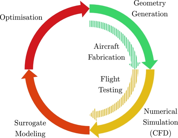
The design loop, shown in Fig. 1, is based on a co-Kriging surrogate model trained with numerically simulated data and data captured during free-flight testing of airframes manufactured through a rapid additive manufacturing process. These two sources of data are fundamentally complementary. Steady-state numerical simulations are conducted in highly constrained and controlled environments. This method of testing allows for the identification of subtle differences in aerodynamic properties across a given set of geometries. Free-flight testing data, which is considerably less deterministic than steady-state numerical simulations, provides physically accurate performance data for an aircraft geometry. Because flight testing provides the most realistic information about aircraft performance, here we will consider it to be the highest fidelity data available. In this work, the additional information gained from flight testing implies that numerically simulated data is viewed as low-fidelity data for the purposes of building co-Kriging surrogate models.
The complete design loop. The outer loop resembles a typical surrogate model driven optimisation process. The addition of the inner loop corrects the numerically simulated data with results of physical experiments.

Co-Kriging excels at producing predictive models with limited data, making it a useful technology for problems where data is costly to obtainFootnote *, such as in merging CFD data with experimental data(Reference Forrester2,Reference Kuya, Takeda, Zhang and Forrester3) . Additionally, Co-Kriging models consolidate multi-fidelity data efficiently; the accuracy of the model significantly improves with the addition of limited high-fidelity data. The resulting model can provide a physically accurate prediction at any point in the design domain. Querying this model takes milliseconds on a standard desktop computer, enabling efficient design search optimisation using global optimisers. This enables the use of these models in platforms such as pyMDO(Reference Martins, Marriage and Tedford4) and pyOpt(Reference Perez, Jansen and Martins5) Footnote **.
The remainder of this paper introduces and discusses the individual elements that comprise this proposed design loop. These topics include a discussion on the state of additively manufactured sUAS, aircraft geometry parameterisation, numerical simulation of sUAS, surrogate model construction and automated flight testing of sUAS. A case study is presented in the final section that demonstrates the application of this design loop.
3.0 THE STATE OF ADDITIVE MANUFACTURING OF AIRCRAFT
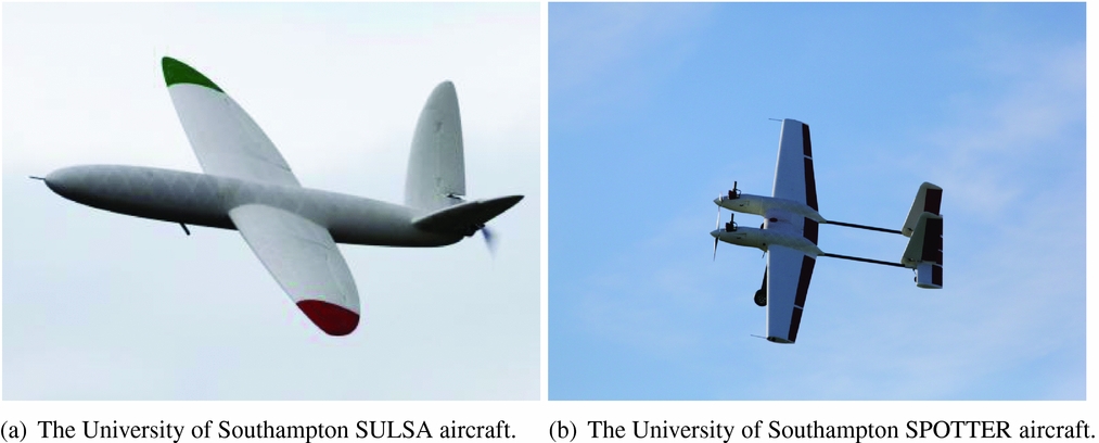
Southampton University Laser Sintered Aircraft (SULSA), see Fig. 2(a), was the first aircraft featuring an airframe wholly manufactured via Selective Laser Sintering, an additive manufacturing technology(Reference Marks6). The aircraft was fabricated in five components and included kinematic joints and locking mechanisms, eliminating the need for fasteners. The SULSA aircraft was a technology demonstrator for additive manufacturing technologies in airframe fabrication. The lessons learned during the design and fabrication have since been integrated into subsequent airframe designs, such as the 3.5 m wingspan Spotter aircraft, Fig. 2(b). Additive manufacturing, specifically selective laser sintering, was extensively used in the fabrication of the fuselage, wings, cowlings and empennage.
Example airframes that used additive manufacturing in construction.

Example geometries produced with Rhino and the parametric wing formulation of Equation (1).

Since SULSA, a number of additional aircraft have been additively manufactured elsewhere. Aurora Flight Sciences demonstrated a 1.6 m wing printed through an Fused Deposition Modelling (FDM) process(7). The MIT Lincoln Lab demonstrated a variable span unmanned aircraft wing fabricated using additive manufacturing(Reference Stern and Cohen8). More recently, the University of Sheffield’s Advanced Manufacturing Research Centre demonstrated a blended wing body glider and powered blended wing body aircraft fabricated via FDM(Reference Nicholson9). These examples are presented as evidence that additive manufacturing of sUAS is feasible.
4.0 AIRCRAFT GEOMETRIES
The method of defining an aircraft geometry is fundamental to this, or any, design and optimisation process. In this work, the geometry engine is required to produce not only high-quality, parametric outer mould lines for numerical simulation but also detailed solid geometries for manufacturing. The geometry engine selected for this design loop is the publicly available AirCONICS platformFootnote * (Reference Sóbester10,Reference Sóbester and Forrester11) . AirCONICS is built on Rhinoceros 5(12) and the OpenNURBS toolkit(13). Rhinoceros 5 is a powerful tool for generating outer mould line surfaces and provides a wide selection of computer aided design tools that can be used to create the solid geometries required for fabrication.
The geometry code used to generate the lifting surfaces of the aircraft at the centre of this paper implements three suggestions from Sóbester(Reference Sóbester10): it uses object-oriented shape primitives, separates the shape definition and scaling properties of geometries and uses a geometry-attached, leading-edge curvilinear coordinate system to define the shape of the geometry.
As an illustration of the concept of the geometry-attached curvilinear coordinate system, consider an axis that is anchored at the root chord and the tip chord of a wing and is coincident with the leading edge of the wing. This axis, which we shall refer to as the ε axis, has a non-dimensional value of zero at the root and one at the tip.
A lifting surface geometry is generated by defining values of sweep, dihedral, twist and aerofoil section as functions of ε. Sweep and dihedral describe the shape of the leading edge of the wing, while twist and chord length define the shape of the trailing edge. The aerofoil cross section is also defined at each point along the ε axis, establishing the outer mould line and the volume of the wing. The description of the wing can be summarised as
 $$\begin{equation}
\mathrm{Lifting\;Surface} = G(\underbrace{{f_{sweep}}({{\epsilon }}), f_{dihedral}({{\epsilon }})}_{\scriptstyle{\rm{Leading \ Edge}}}, \overbrace{f_{twist}({\epsilon}), f_{chord}({\epsilon})}^{\text{Trailing Edge}}, f_{section}({\epsilon })).
\end{equation}$$
Each function f must be smooth and continuous for ε ∈ [0, 1]. The function can take any form, from a constant value to a piecewise function, allowing for a broad range of geometries.
Two additional parameters control the scaling of a non-dimensional shape to a fully dimensioned wing: a scaling factor applied to the entire geometry (this scales the geometry whilst preserving the shape of the wing) and a separate scaling factor applied to the chord length, called the chord factor.
Wing properties, such as span, planform area, wetted area and aspect ratio, may be used as design variables in wing optimisation. The relationship of the chord and scale factor to these metrics depends on the mathematical description of the wing shape (Equation (1)). For certain geometries, an analytical solution exists to relate the aforementioned geometry scaling factors to the parameterised wing properties, like planform area and aspect ratio. However, not every geometry offers an obvious analytical mapping between them. In such cases, these parameters can be found via a numerical method – effectively a low level, internal optimiser. As we aim for generality here (after all, the freedom to use a wide variety of shapes is one of the unique selling points of additive manufacturing) we adopt this more generic approach of using a local search to identify these parameters in this work.
The Python programming language is used internally in Rhinoceros 5 to generate geometries (defining the geometry as a script), allowing external libraries to be imported for use. The search for the optimal chord factor and scaling factor is conducted using the optimisation toolkit of the Scipy package(Reference Jones14). We use the Nelder-Mead simplex algorithm(Reference Nelder and Mead15) to modify the two scaling factors of the wing to obtain the target aspect ratio and wing area. The objective function for this optimisation is an aggregate of two separate functions, one for the area and one for the aspect ratio. The optimal scaling factors produce a wing that is defined in both shape and scale.
We use Rhinoceros 5 to generate all necessary files for computer simulation and manufacturing. Additionally, the Rhinoceros 5 model calculates the key geometric properties of the aircraft wing, such as surface area, mean chord length, volume and planform surface area. These values and the wing geometry represent a complete set of geometry data that can be evaluated with numerical methods or flight testing.
5.0 NUMERICAL SIMULATION OF THE FLOW AROUND AN AIRCRAFT
Once the digital geometry has been generated, the aerodynamic merit of the design must be established. OpenFOAMFootnote * was selected as the Reynolds-Averaged Navier-Stokes (RANS) solver for generating numerically simulated data. SimpleFOAM, one of the solvers within OpenFOAM, was used for steady-state incompressible turbulent flow simulations using an SST k − ω turbulence model. Meshes were constructed using the OpenFOAM SnappyHexMesh mesh generation software. SnappyHexMesh allows for control of curvature refinement and boundary-layer additions, both of which were employed in these simulations. While the final mesh cell count depends on the underlying aircraft geometry, the typical mesh would consist of between 7 million and 7 million cells.
Because this design loop requires the numerical simulation of a large number of geometries, we needed to automate the simulation process. A software package, droneCFDFootnote **, was written to automate the tasks of pre-processing, meshing, simulating and post-processing data. droneCFD automatically configures the simulation, pre-processes the model, generates and meshes the simulation domain and runs the simulation. Command line arguments allow a user to specify many attributes of the simulation, including the angles of attack (AoAs). droneCFD uses a steady-state solver, such that each simulation converges on a numerical estimate for the lift and the drag for an aircraft geometry. For this design loop, each aircraft geometry is tested at five AoAs. The sUAS considered in the paper typically operate at Reynolds numbers of around 70,000 to 150,000. The Reynolds number of each of the simulations described here is fixed at a root chord Reynolds number of 120,000.
A simple aerodynamics model of the aircraft is created using the computational fluid dynamics results thus obtained. The model consists of an equation that describes the lift coefficient (Equation (2)) and one to model the drag coefficient (Equation (3)) of each design as a function of the AoA.
 $$\begin{equation}
L_f(\alpha , v) = qS (m\alpha + C_{l_0}),
\end{equation}$$
 $$\begin{equation}
D_f(\alpha , v) = qS ( m_1\alpha ^2 + m_2\alpha + C_{d_0}),
\end{equation}$$
where q, or the dynamic pressure, is calculated as q = ρv 2/2.
This model depends on five variables,
 $m, C_{l_0}, m_1, m_2 \;\text{and } C_{d_0}$
, which are unique to each aircraft geometry. These parameters can be extracted easily from the numerically simulated data, and, as we shall see shortly, also from free-flight testing, making these parameters ideal for demonstrating this design loop.
Once these model values have been identified, the steady and level cruise performance and optimal flight condition of the aircraft can be determined. For an aircraft to be at cruise, the lift force, L 0, generated by the wing must be equal and opposite to the gravitational force acting on the aircraft. This constraint leads to a limited number of flight conditions this aircraft can operate in, being primarily driven by the AoA and the cruise airspeed. The optimal flight condition for this aircraft is assumed to be the point where the drag is at a minimum.
Given that both D f (α, v) and L f (α, v) have smooth and continuous first partial derivatives, a constraint condition can be added to the lift function. Equation (2) is converted into an equality constraint, adding a term for the desired lift force, or L 0, and setting the function equal to zero:
 $$\begin{equation}
L_{f_c}(\alpha , v) = q (m\alpha + C_{l_0}) -L_0 = 0
\end{equation}$$
This function depends only on α and v. Solving Equation (4) for α produces
 $$\begin{equation}
\alpha = - \frac{\left(\mathrm{A}\, C_{l_0}\, \rho \, v^2 + 2\, \mathrm{L_0}\right)}{A\, m\, \rho \, v^2}
\end{equation}$$
This can now be substituted into Equation (3):
 $$\begin{equation}
D_f(v) = \frac{\mathrm{A}\, \rho \, v^2}{2}{\, \left(C_{d_0} - \frac{m_2\, \left(\mathrm{A}\, C_{l_0}\, \rho \, v^2 + 2\, \mathrm{L_0}\right)}{\mathrm{A}\, \mathrm{m}\, \rho \, v^2} + \frac{\mathrm{m_1}\, {\left(\mathrm{A}\, \mathrm{c_{l_0}}\, \rho \, v^2 + 2\, \mathrm{L_0}\right)}^2}{\mathrm{A}^2\, \mathrm{m}^2\, {\rho }^2\, v^4}\right)}.
\end{equation}$$
Differentiating the right-hand side of Equation (6) and setting it to zero locates the critical points of the function, allowing the minimum drag condition to be identified. The AoA can be found by evaluating Equation (5) at the velocity obtained for the minimum drag force.
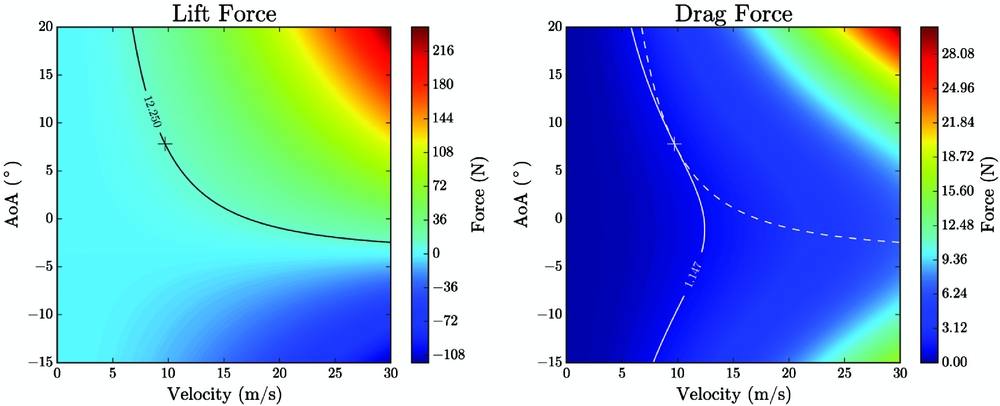
These analytical solutions can be visualised by plotting Equations (2) and (3). Figure 4 shows two contour plots, one indicating the lift force and one showing the drag force. The lift force has a single black contour line, indicating a range of values that produce the correct lift for the aircraft (which is 12.25 N the example is shown in Fig. 4). The lift contour line is projected onto the drag plot as a dotted line. The solid white contour line shows a drag contour that is tangent to the lift contour, indicating a minimum value. The + indicates the analytical solution obtained from the equations above.
Contour plots of Equations (2) and (3) used for the determination of optimal aircraft performance.

This completes the process of numerically simulating an aircraft. The next step is to collect these numerically simulated data into a single model that provides an understanding of the entire design region. The task of converting discrete simulations into a predictive model is left to a Kriging surrogate model – this is the aspect of the design loop we turn our attention to next.
6.0 SURROGATE MODELLING
Surrogate models are a powerful means of learning the response of a physical system from a limited number of discrete data points, typically obtained through expensive numerical or physical experimentation. This section is dedicated to a discussion of the creation, training and refinement of surrogate models. The creation of a surrogate model begins with the design of a sampling plan. Each point in this sampling plan describes a vector that comprises the design variables of the aircraft geometry. The ideal sampling plan is one that contains the number of sampling points that matches the available computational budget and that fills the design space uniformly. In this work, Morris-Mitchell optimised Latin hypercubes are used(Reference Morris and Mitchell16). In our proposed design loop, each point in the sampling plan is evaluated using numerical simulation, and some subset of the initial population is selected for fabrication and flight testing. The resulting data are used to train a co-Kriging surrogate model. For details on the mathematical formulation and process of creating a co-Kriging model, we recommended Jones(Reference Jones17) and Forrester et al(Reference Forrester, Sobester and Keane18).
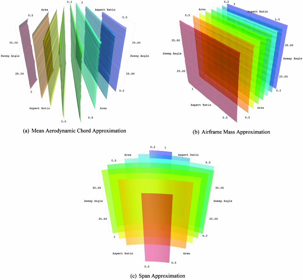
For the case study presented in detail in Section 8, an initial sampling plan was created with 150 points. The box-wing aircraft is parameterised by three design variables: aspect ratio, planform area, and wing sweep. The digital geometry for each point is created in AirCONICS and evaluated using droneCFD. The polynomial aerodynamics model introduced in the last section requires five unique parameters. This variable count means that five individual surrogate models are produced in this design loop, one model for each aerodynamic coefficient. Once trained, these five models will predict the C l (α) and C d (α) curves for any point in the design domain. Three additional surrogate models trained using data related to geometric characteristics of the aircraft for use in the optimisation process. These three models allow for the approximation of span, mean aerodynamic chord and airframe mass (calculated using the volume of the additive manufacturing ready AirCONICS model and density of the fabrication material), based on only the design vector of a parameterised aircraft without the instantiation of a new AirCONICS geometry model. This becomes useful in stochastic optimisation, because it reduces the approximation of these properties from a few seconds of wall time per evaluation (using an AirCONICS model) to tens of milliseconds per evaluation (using a surrogate model).
A Genetic Algorithm, specifically the NSGA-II(Reference Deb, Pratap, Agarwal and Meyarivan19), is used to identify the optimal hyper-parameters for each of the eight models. These hyper-parameters provide insight into the response of the model for each design variable. The initial fit provides valuable information about where a model lacks sufficient information to generate accurate predictions. The task of identifying and adding data to a surrogate model is often referred to as ‘generating infill points.’
When the initial sampling plan is generated, the only objective is to create a space filling set of points. This is because no information about the response of the model is known at this stage. Once the training of the initial surrogate model is complete, additional information is available for adding points that can beneficially affect the usefulness of the model. The method used to improve the model largely depends on the desired outcome. The surrogate models discussed in this work are used to provide predictions at sites left un-sampled by the costly CFD analysis. Therefore, they require a consistent accuracy across the domain.
An accurate model is one that exhibits a low mean-squared prediction error estimate over the entire design domain. For the general improvement of a model, a search can be performed that identifies regions of significant error, which is driven by the Euclidean distance between points and the hyper-parameters of the model. When such an area is found, a sample point can be added, and the model retrained. This process is repeated for several iterations until the computational budget is exhausted, or the model reaches the desired accuracy. If points are to be added in parallel, imputation may be used in the selection of points to choose.
Imputation is the process of temporarily allowing a predicted value at a point in the model domain to be considered as a valid observation. This method is used in situations where multiple infill values are added to a model in parallel. Adding the predicted value into the model modifies the mean-squared error distribution of the model without requiring retraining of the hyper-parameters. This allows for the selection of the next most significant error source in the model. Each temporary value is replaced with the observed value after the evaluation is complete, and the model is retrained to reflect the addition of new information in the model.
Imputation assumes additional significance when several surrogates are being trained simultaneously. The selection of a point in one model impacts the choice of infill location in the other models (four in our case). In this work, the mean error of each model is established and is used as a ranking to guide the infill process. A 500-point random latin hypercube is created to determine the average mean-squared error of each model. The mean-squared errors are computed at each point for the five models,
 $m, C_{l_0}, m_1, m_2 \;\text{and } C_{d_0}$
, and the values are averaged. The model with the highest overall error is selected to choose the first infill point while the most accurate model is last to pick an infill point.
7.0 AUTOMATED FLIGHT TESTING AND AERODYNAMIC PERFORMANCE EVALUATION
This section discusses the techniques used in this study to collect aerodynamics data from small unmanned aerial vehicles during flight testing. Because these data are directly compared to the aerodynamics models generated from simulated data, the type of the data collected must be of the same type as the aerodynamics data gathered from CFD simulations.
7.1 Instrumentation for flight testing
The Flight Management Unit (FMU) of an autonomous sUAS handles control and navigation. Microelectromechanical Systems (MEMS) technologies have enabled the miniaturisation of flight management units for sUAS. MEMS sensors were first explored for missile guidance systems(Reference Ruffin20) before being applied to sUAS flight management units(Reference Jang and Liccardo21). The number of MEMS-based autopilots has increased quickly(Reference Chao, Cao and Chen22). A complete flight control system, with MEMS sensors, GPS, and telemetry downlinks are now commonly available for approximately $300Footnote *.
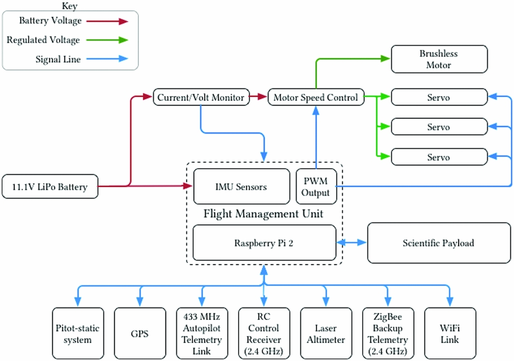
The hardware used for the experiments described here represents the state-of-the-art for low-cost flight management units. The central processing unit is a Raspberry Pi 2, running a real-time Linux kernel. GPS, inertial data, and radio control inputs are supplied by the Navio+ board mounted on the Raspberry Pi. A schematic of the specific hardware system used here is shown in Fig. 5.
The unmanned aircraft system used for flight testing.

This flight management unit runs the open-source ArduPlane softwareFootnote **. This software, first released in 2007, has acquired a wide user base and is under active development. While this software was originally designed to be run on 8-bit microcontrollers, significant development work has been completed to make the software portable across many platforms, including the ARM processors used in the Raspberry Pi 2. The ability to use high-performance processors has led to the development of sophisticated sensor fusion and control algorithms. ArduPlane currently employs an advanced Extended Kalman filter for sensor fusion and state estimation. Additionally, the current generation of flight management unit software allows for real-time access to flight data and the parameters that determine how the flight management unit controls the aircraft.
Programmatic access to the parameters that control the flight management unit, as well as the current attitude data for the aircraft, are available through a Python interface. This programmatic interface allows for high-level scripting of the flight tests described in the next section. Safety is the primary concern when using a programmatic interface to the flight management unit. The process of developing flight testing procedures begins in a software-in-the-loop testing environment. This environment allows the script to be run for hundreds of flight hours. This method of testing is used to identify any software interaction issues that would cause unsafe operations during physical flight testing. Once the script passes the software-in-the-loop environment testing, the script is moved to the aircraft.
While a script is running, an independent safety system is run that can automatically abort the flight testing should any anomalies be detected. This system monitors the vital statistics of the aircraft, looking for any parameter that falls outside of its acceptable range. For example, if the telemetry radio signal strength drops below an acceptable level, the test is terminated. Should something unexpected happen during an aerodynamics flight test, the flight management unit reverts to the last known stable configuration and returns to a loiter over the launch position. Finally, a professional pilot, in visual line of sight at all times, monitors the flight. The pilot can override the flight management unit with a switch on a radio control transmitter and return the aircraft to the launch location safely.
7.2 Flight test method
The goal the of flight testing described here is to measure the aerodynamic performance of a prototype, as part of an iterative design process. High-resolution behaviour data is supplied by the flight management unit, which records and logs every aspect of the aircraft system. An unpowered glide test was used to extract the aerodynamics data needed.
A racetrack pattern of waypoints is used to conduct a gliding test, as shown in Fig. 6. Specifically, the pattern is used for glide slope testing. Navigation waypoints are indicated by circles and the waypoint number is shown inside the circle. The aircraft enters the circuit at waypoint one. Here, the onboard computer sets the airspeed target for the aircraft. The flight management unit is instructed to maintain a particular airspeed during the descent, which changes during each circuit of the racetrack pattern. This method leads to data collected at a broad range of pitch angles and glide slopes. At waypoint two, once the aircraft has converged on the requested airspeed, it is instructed to enter an unpowered glide. At waypoint three, full power is restored to the aircraft and the airspeed is set to cruise. Waypoints four and five are included for navigational purposes only. The number of waypoints and the shape of the actual flight trajectory varies based on flying location and wind conditions, but the concept of each flight plan is the same.
The flight path used for glide slope identification testing.

The flight management unit configuration requires alterations to conduct these glide tests. The ArduPlane software has an internal energy management scheme known as TECS, or the Total Energy Control System. In typical autonomous operation the TECS system manages the altitude of the aircraft, airspeed, and throttle. The objective functions of the TECS system are an error metric for altitude and an error metric for airspeed, which it seeks to minimise. As altitude and airspeed may be competing objectives, the flight management unit attempts to balance altitude errors and airspeed errors.
During gliding flight, the flight management unit accumulates a significant altitude error while the throttle is disabled. If left in a normal operating mode, the aircraft will sacrifice airspeed in an attempt to regain altitude. This behaviour leads to a feedback cycle that causes the aircraft to pitch up and down during flight, and may cause a stall. To prevent this, the flight management unit is instructed to ignore altitude errors during the testing phase of the flight. Once the test leg of the flight is completed, these parameters need to be reset to the normal operating condition, as maintaining altitude is critical to safe flight operations.
7.3 Flight testing data processing
Once a test flight is completed, the data recorded by the flight management unit can be processed to extract the C l and C d polars of the aircraft. We extracted the parameters using techniques inspired by work on motion tracking(Reference Cory and Tedrake23-Reference Uhlig and Selig25) and flight testing(Reference Li, Hoffer, Stark and Chen26-Reference Sørensen, Blanke and Johansen29). Uhlig and Selig(Reference Uhlig and Selig25) outlined a method for converting trajectory information into aerodynamic data for micro air vehicles, which was used to post-process the data from the Inertial Measurement Unit (IMU) of the aircraft.
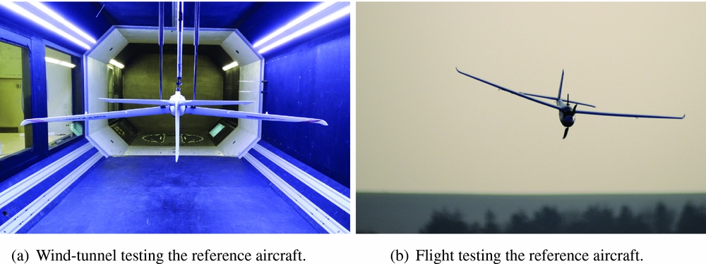
While the additive manufacturing process for fabricating the aircraft discussed in Section 8 was being developed, initial flight testing was conducted using a modified off-the-shelf sUAS. This sUAS, which was both flight tested and wind-tunnel tested, allowed for the verification of the data extraction methods outlined above. This aircraft, shown in Fig. 7(b), provided a stable platform for the development of the onboard software and for quick testing of data collection. This aircraft performed the glide test manoeuvres described above and used the same FMU and sensors as the parametric aircraft that forms the object of the case study in Section 8, demonstrating the design loop proposed here.
Collecting data from the reference aircraft to validate the IMU data extraction.

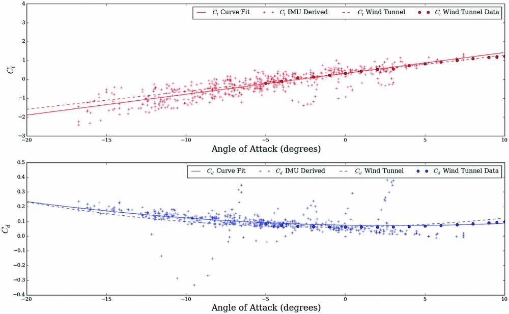
A comparison of flight test and wind-tunnel test data is shown in Fig. 8. The dotted lines indicate a polynomial fit of two wind-tunnel tests. The solid lines indicate the fit to the flight test observed data, indicated by the ‘+’ symbols. The fitting process of the flight test data starts with generating an initial guess for the curve fit. For this test, these values were taken from the wind-tunnel data curve fit. The results show good correlation to wind-tunnel data, although the noise in the C l measurement is significant.
A comparison of flight testing results to wind-tunnel tests. The dashed lines represent wind-tunnel testing, the solid lines represent a polynomial fit of the flight data and the + symbols represent IMU observations. As the IMU generates a significant number of observations, only one in 20 data points are shown here for plot clarity. These points were selected using a pseudo-random number generator.

Advances in intelligent aircraft structures, such as distributed sensor networks(Reference Salowitz, Guo, Nardari, Li, Kim, Kopsaftopoulos and Chang30,Reference Kopsaftopoulos, Nardari, Li, Wang, Ye and Chang31) , should dramatically improve the ability to perform this type of a flight testing activity. Kopsaftopoulos et al(Reference Kopsaftopoulos, Nardari, Li, Wang and Chang32) demonstrated AoA determination using wing-embedded pressure and strain sensors in a composite wing. Distributed sensors may soon be fabricated directly into the aircraft using additive manufacturing(Reference Lopes, MacDonald and Wicker33-Reference Espalin, Muse, MacDonald and Wicker37). These technologies, and other similar technologies under development, will further advance the ability to determine the aerodynamic performance of an aircraft in flight.
8.0 APPLICATION OF THE DESIGN LOOP
We demonstrate the methodology proposed here on an example sUAS: a jointed wing parametric aircraft, an additively manufactured instance of which is shown in Fig. 19. This aircraft is parameterised with three variables: aspect ratioFootnote *, planform area and sweep angle. Table 1 lists the ranges for each of these variables used for simulation.
Box-wing design parameters with upper and lower limits used in the demonstration of the design loop

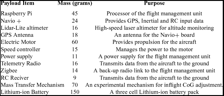
The total mass of the flight payload is 450 g. The payload contains a laser altimeter for terrain mapping and a novel system for adjusting the centre of gravity of the aircraft in flight, a detailed breakdown can be found in Table 2.
The payload of the aircraft considered in this design loop

An optimal Latin hypercube of 150 points was selected as the initial sampling plan to generate the initial low-fidelity surrogate model. The outer mould line geometries for each point in the sampling plan were instantiated from a parametric model defined in AirCONICS and evaluated with droneCFD. The post-processed data was collected and the initial model was trained. An additional 120 infill points were added to the model. To expedite this process, imputation was used to select parallel infill points. Three consecutive sets of 40 points each were selected for evaluation. The model was retrained after the complete evaluation of each set of 40 points.
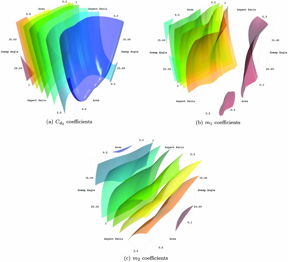
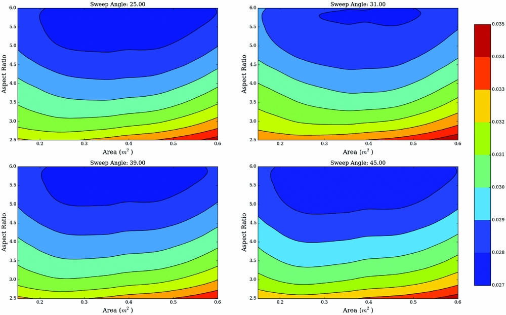
The models based on numerically simulated data are shown in Figs. 9–11. The plots show fixed-value iso-contours of the surrogate models. These plots demonstrate the complex interactions between the design variables for each modelled parameter. Each plot is captioned by the aerodynamic coefficient the plot represents. Additionally, Fig. 12 shows four 2D contour plots of C d 0 . These plots show the same data as Fig. 9, but sliced at four fixed sweep angle. The formulation of the aerodynamic model has been repeated here in Equations (7) and (8) for quick reference:
 $$\begin{equation}
L_f(\alpha , v) = qS (m\alpha + C_{l_0}),
\end{equation}$$
 $$\begin{equation}
D_f(\alpha , v) = qS ( m_1\alpha ^2 + m_2\alpha + C_{d_0}),
\end{equation}$$
where q, or the dynamic pressure, is calculated as q = ρv 2/2.
Drag coefficient surrogate models trained with data from CFD data.

Lift coefficient surrogate models trained with data from CFD data.

Geometry property surrogate models trained with data from CAD generated data.

These sliced 2D plots show data from the C d 0 Kriging model at fixed sweep angles of 25°, 31°, 39° and 45°.

Once the surrogate models are constructed, a multi-objective optimiser is used to identify designs optimally suited for the payload listed in Table 2. The chosen design will be the first aircraft manufactured for flight testing. Equation (9) summarises the optimisation formulation used in this design loop.
 $$\begin{equation}
\begin{array}{l@{\quad \;}l} {\text{minimise}}_{{\bf x}} & F_{drag}({\bf x})\,\,, \alpha ({\bf x}) \,\, \text{and}\,\, v_{cruise}({\bf x}),\\
\text{such that} &F_{lift}(\mathrm{\mathbf {x}}) - F_g(\mathrm{\mathbf {x}}) = 0,\\
\text{and} & b_{max} - b({\bf x}) > 0,\\
\text{and} & Re(\mathrm{\mathbf {x}}) - Re_{min} > 0,\\
\text{and} & \alpha _{max} - \alpha (\mathrm{\mathbf {x}}) > 0,\\
\text{subject to} & x_i \in [x_i^L,x_i^U]\hspace*{60pt} i = 1,2,\ldots ,n. \\
\end{array}
\end{equation}$$
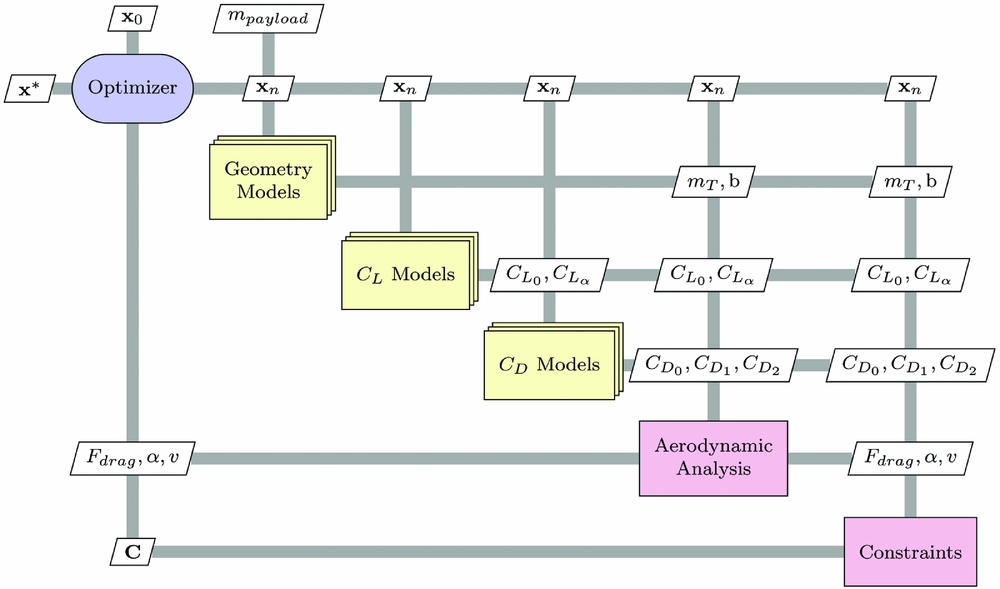
Three objectives are explored: minimising the drag force of the aircraft at cruise, minimising the AoA of the aircraft at cruise and minimising the airspeed of the aircraft. An equality constraint on the lift force of the aircraft is used to ensure the aircraft is operating in steady level flight. Three inequality constraints are placed on this optimisation: the span must be no greater than 2 mFootnote *, the chord Reynolds number at cruise must be greater than 100,000Footnote ** and the AoA, α, must be small such that the optimiser does not design an aircraft that operates near the stall point of the wing. As the aircraft is operating in low Reynolds number conditions, the maximum allowed AoA is α max ≈ 8°. A summary of the optimisation process is shown in Fig. 13.
A graphical flow chart of the design loop optimisation process. This figure follows the guidance as outlined by Lambe and Martins(Reference Lambe and Martins39).

This optimisation is conducted with the NSGA-II multi-objective optimiser. On a standard desktop computerFootnote † , the optimisation process requires less than 5 min. The only input variable to the process is the payload mass, in this case 450 g. For each design considered, the optimiser begins by building a mass estimate for the airframe. This mass comes from the solid geometry files created during the evaluation of outer mould line geometries for numerical simulation. The sum of the airframe mass and the payload mass is the required lift force of the aircraft. This required lift force is used to formulate the lift constraint function, Equation (4). Each of the five aerodynamic coefficient surrogate models is queried to supply the necessary information to identify the optimal cruise condition. Once the drag force, the optimal AoA and the cruise velocity are determined, the constraint conditions of the optimiser are evaluated. These objective and constraint data are returned to the optimiser.
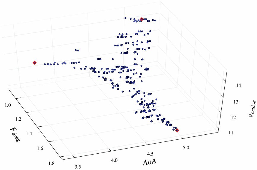
The optimiser is run with a population size of 150 for 100 generations. The NSGA-II used a tournament selection for cross-over, and random Gaussian mutations are set to occur at a rate of 5%. Fig. 14 shows the Pareto-optimal results from the optimisation. The design selected for fabrication from these results was the one with the lowest Euclidean distance to the minimum observed values of the set. Each design variable is first normalised, such that the magnitude of the of the objective does not bias the selection of the optimal design.
The Pareto front resulting from a multi-objective optimisation. The square markers indicate the best designs for each design variable, and the star indicates the aircraft design nearest the Utopian point.

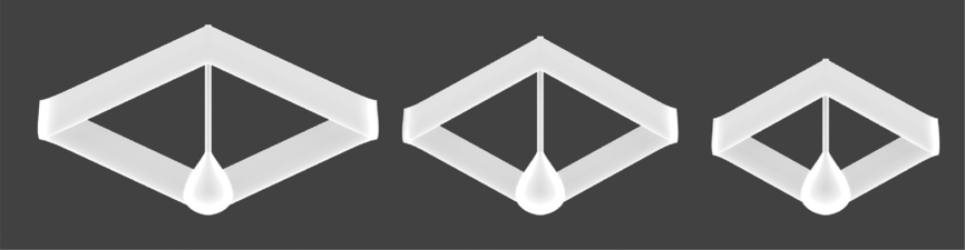
Three aircraft were selected from the Pareto front shown in Fig. 14. Aircraft 1 was selected by identifying the utopia point in the model. Two additional aircraft were selected by modifying the weighting factors of the importance of two variables: cruise velocity and drag force. These two variables were selected as factors likely to impact the scale and shape of the aircraft. Ultimately, the desired outcome of this weighting scheme is to select two aircraft that have performance similar to Aircraft 1, but have different geometry properties. These aircraft are called Aircraft 2 and Aircraft 3, respectively. The corresponding design vectors can be found in Table 3. A visual comparison of the aircraft can be found in Fig. 18.
A summary of aircraft selected for flight testing

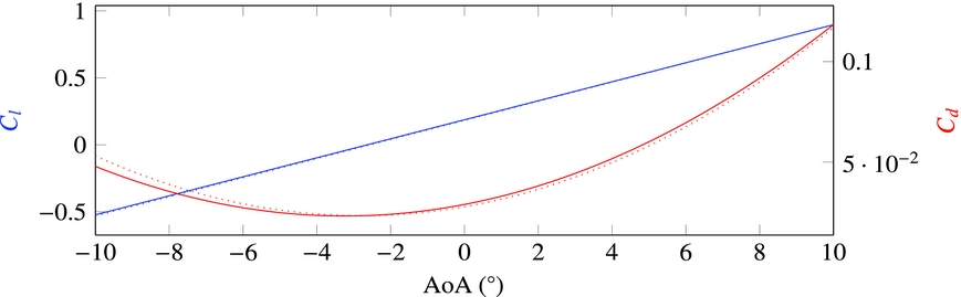
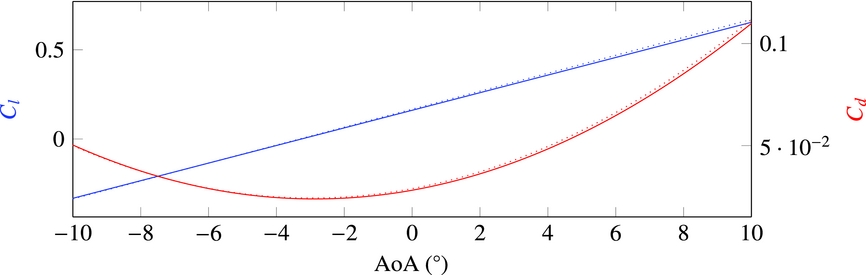
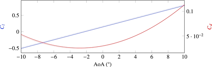
Once the three aircraft were selected for flight testing, new OML geometries were generated and numerically simulated to validate the prediction of the model. The results of the simulations are shown in Figs 15–17. In these three figures, the results the OpenFOAM RANS solver are plotted against the Kriging model predictions. These curves show good agreement. This gives confidence in the predictive capabilities of Kriging models and the optimisation results.
Surrogate model prediction compared with the simulated results for Aircraft 1.

Surrogate model prediction compared with the simulated results for Aircraft 2.

Surrogate model prediction compared with the simulated results for Aircraft 3.

CAD renderings of the aircraft selected for flight testing. Aircraft 1 is on the left, Aircraft 2 in the middle and Aircraft 3 is on the right.

The aircraft were constructed using a number of additive manufacturing technologies. The wings were fabricated primarily using FDM. The fuselage was fabricated using ink jet deposited UV curable materials, and parts of the empennage were fabricated using a Stereo Lithography Apparatus (SLA). The fabrication files for these aircraft were generated using a modified version of the AirCONICS platform that allows for the generation of three-dimensional solids.
Additive manufacturing simplifies the fabrication of these aircraft but introduces unique material considerations. The primary concern in fabricating an aircraft is the strength and mass of the airframe. The polymers used in the construction of these aircraft have a density of approximately 1 g/cm3.
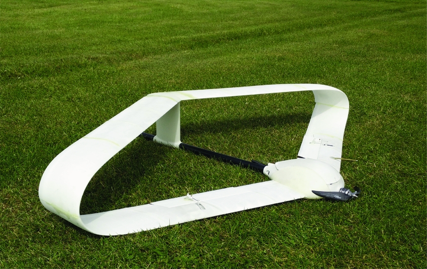
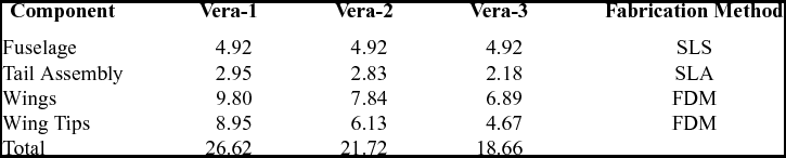
Commercially available Selective Laser Sintering (SLS) services often require wall thicknesses of 0.8 mm for components made of sintered nylon. VERA-1 was first fabricated using this technology with a skin thickness of 1 mm. The resulting aircraft was robust but had a higher than desired mass. The SLS version of VERA-1 is pictured in Fig. 19. The next iteration of VERA-1, as well as VERA-2 and VERA-3, were fabricated using FDM. In the FDM process, the skin thickness is controlled by the diameter of the extrusion nozzle. For the three aircraft flown here, a wall thickness of 0.3 mm was achieved, resulting in lightweight structures. Additional internal supports were necessary to improve the robustness of the wing segments. Additionally, two carbon fibre spars were included in the wing sections. Two hollow 4 mm carbon fibre rods are placed at 10% Mean Aerodynamic Chord (MAC) and 60% MAC. These tubes extend from the fuselage to the curved joined wing of the aircraft, and again from the tail of the aircraft to the curved joint of the wing. The carbon fibre tubes used in this construction of these aircraft have a mass of 10 g/m. The control surfaces of these aircraft were fabricated from commercially available balsa wood trailing edge. The hinge of the aircraft was constructed using fibre reinforced tape. The total time required to make and assemble each aircraft was around 30–40 h wall time, of which 20–30 h was the time needed for additive manufacturing. A summary of fabrications times for the various fabrication runs required to fabricate these aircraft can be found in Table 4. These figures indicate wall time to fabricate and build several aircraft for this application of the design loop. These wall time figures could be improved significantly. Assembly times can easily be reduced with additional design development component interconnects. The fabrication time of the aircraft could also be reduced. The specific mechanism for reducing the wall time depends on the method of additive manufacturing used. For FDM, additional equipment allows for the production of parts in parallel, reducing wall time. In SLS, several aircraft could be fabricated in the same run, reducing the wall time per aircraft.
The SLS fabricated version of Aircraft 1.

Aircraft fabrication time breakdown

After fabrication, these three aircraft were flight tested. Each aircraft flew at least three times. The first flight was a flight management system tuning flight. The flight envelope of the aircraft is also tested during the first flight. Airspeeds were of specific interest here, as the flight envelope of the aircraft needs to be established. The second flight of each aircraft was a largely autonomous flight of the aircraft in which the flight management unit was allowed to conduct the glide testing routine described in Section 7. The third flight was used for validation of the second, and to correct any problems.
The manufacturing of the blended wing shape using additive manufacturing modifies how mass is distributed in the aircraft. The curved portion of the wing tips have a mass of a few hundred grams, or approximately 25–35% of the mass of the wings. In a conventional planar wing, this is mass that would not be present (unless wing tip fuel tanks are used). In the box-wing structure, the increased mass at the wing tips may modify the roll moment of the aircraft. An increase of roll moment requires careful control of the aircraft in flight. As a precaution, the sUAS tested here were constrained to bank angles of no more than 20°. Additionally, the maximum roll rate of the aircraft was set to 40° s−1 to prevent sudden rolls during navigational turns. The waypoints for the test flight were assigned such that no turn greater than this roll angle would be required. Additionally, great care was taken to fly these aircraft on days with calm conditions to reduce the impact of weather on the dispersion of the data.
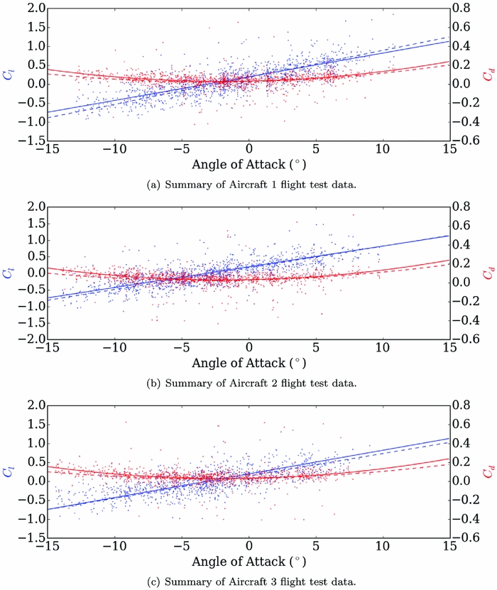
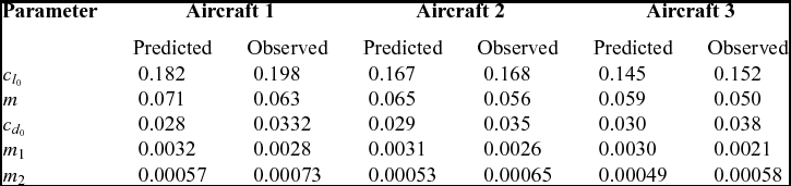
The results of the flight testing are shown in Fig. 20 and summarised in Table 5. In Fig. 20 , the dotted line represents the prediction, data points represent data collected during the flights, and the solid lines indicate the regression fit of these flight test data. One in every 20 data points is plotted here for clarity. In general, the flight tests agree well with the predicted results. The numerical simulation model shows an underestimate of drag and an overestimate of lift in every model. This is partly due to sources of parasitic drag present on the real aircraft, but not modelled by the simulation: servo arms, control linkages, and antennae. Additionally, because these aircraft were not monolithically fabricated, joints and other assembly artefacts add to the total drag of the aircraft.
Flight test data for the three selected instances of our parametric model.

Summary of predicted and observed results

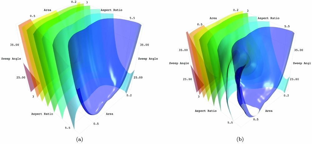
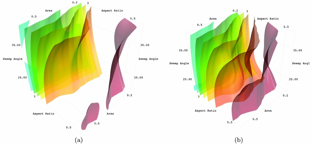
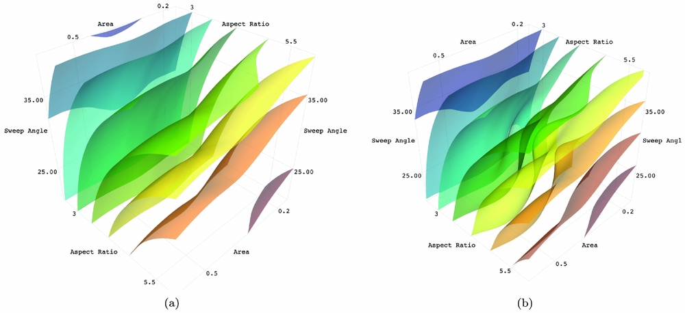
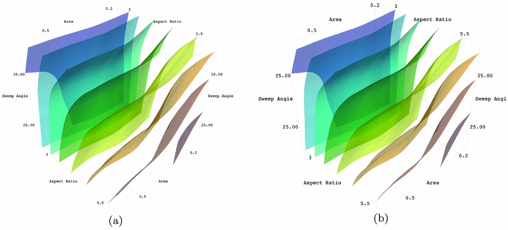
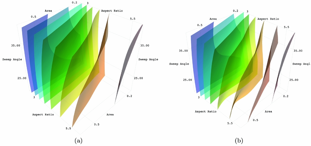
The results from flight testing allow for the construction of a co-Kriging surrogate model. The goal of co-Kriging is to build a model that is globally more accurate in the predicted outcome than a model trained solely with low-fidelity data. To achieve this, a second model is constructed that contains information about the difference between the observed low-fidelity data point and a high-fidelity observation made at the same point in the model. This second model describes the offset at any location in the model between the low-fidelity data and what the expected high-fidelity observation would be. Every prediction from the co-Kriging model is, in effect, a prediction of the low-fidelity model combined with a predicted offset. A comparison of the Kriging and co-Kriging models is shown in Figs. 21–25. In each of the aforementioned figures, the plot shown in panels (a) is the result of Kriging trained using only numerically simulated data obtained from post-processing CFD data. The plot shown in panels (b) shows co-Kriging models that are trained with both numerically simulated data and flight test data.
Co-Kriging Results for C d 0 coefficient, models trained using only numerically simulated data is shown in (a), co-Kriging is shown in (b).

Co-Kriging results for m 1 coefficient, models trained using only numerically simulated data is shown in (a), co-Kriging is shown in (b).

Co-Kriging results for m 2 coefficient, models trained using only numerically simulated data is shown in (a), co-Kriging is shown in (b).

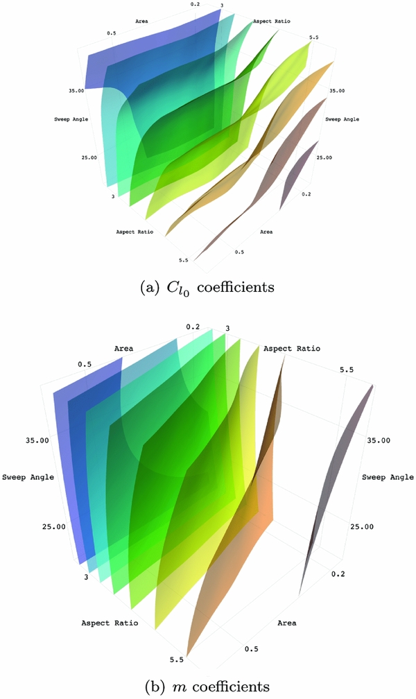
Co-Kriging results for C l 0 coefficient, models trained using only numerically simulated data is shown in (a), co-Kriging is shown in (b).

Co-Kriging results for m coefficient, models trained using only numerically simulated data is shown in (a), co-Kriging is shown in (b).

The iso-contour plot was selected to show how the Kriging model varies with the addition of high-fidelity data. These differences in the shapes of these iso-contours, which is obvious in certain models and less obvious in others, is due to the addition to high-fidelity data. These changes represent the correction of numerically simulated data with flight testing data. As almost all predictive models, the ability to make accurate predictions depends on the amount of information contained in the model. Additional test flights of new aircraft would continue to improve the results presented here.
This case study of the proposed design loop demonstrates how to build a predictive model that allows reasonable predictions of physically accurate results in milliseconds. This rapid prediction capability enables efficient and fast optimisation of new sUAS that can be additively manufactured. While the data collected here was specific to one payload configuration, this model is constructed in such a way that many other payloads can be considered. Additionally, with these data, several types of optimisation are possible. Aircraft may be optimised for endurance, range or other metrics suitable for a particular mission profile.
This design loop was envisioned as a way to reduce the time required to construct new aircraft. Optimisation using the design loop occurs in minutes (wall time) and the fabrication time necessary for a flight-ready aircraft is around 30 to 40 h. Each new design draws information from a library of previous numerical simulations and flight tests, reducing the need to recreate these data. Because the aircraft topology may not be obvious for a particular mission, multiple parameterised aircraft models may be considered in the optimisation process (though the ideal solution may be to parameterise the topology too). This approach represents a significant decrease in design time and allows engineering teams to explore wider design spaces and a broader range of aircraft topologies for sUAS. Because the time between initial design conception and flight testing is short, airframes can be iterated quickly. The result is an efficient design process that produces an aircraft that satisfies the expectations of the design team.
The results presented here demonstrate the potential of the design loop proposed in this paper. For future work, two key questions remain: what density of high-fidelity data is required for physically realistic predictions and how does this required data density depend on the accuracy of the low-fidelity data source. The first question is answered by building and flying additional aircraft. Based on flight test results it is possible to ascertain information about accuracy though model convergence monitoring and cross-validation methods. The second question could be answered by replacing the RANS data presented here with a different source of low-fidelity data. An example of changing data fidelity would be to use, for example, full potential code in place of RANS. Answers to these questions will lead to recommendations as to how best to train and use the design loop proposed here.
9.0 CONCLUSIONS
We introduced a novel design loop that integrates numerically simulated data and free-flight data into a single model for optimisation. This design loop demonstrates the benefits of closely coupling high-performance computing and additive manufacturing in the development and optimisation process of an sUAS. A case study of the application of the design loop demonstrates that an optimal aircraft for a bespoke payload can be optimised in under 10 min, once the initial low-fidelity surrogate model is constructed using numerically simulated data. This identified design can be fabricated with additive manufacturing and flight tested, a process that can be completed in approximately 1–2 days. The data observed from flight testing that aircraft can be used to generate co-Kriging models, improving the overall accuracy of existing Kriging models. These data can then be used to develop and test new, bespoke airframes for a range of payloads and mission applications. These aircraft can likewise be designed and fabricated in 1–2 days so rapid design iterations can be made. The work presented here outlines the foundation of this design loop, and demonstrated one instance of the design loop being used for the design of a box-wing aircraft. Future work will focus on studying the required density of high fidelity in the co-Kriging models of the design loop.
ACKNOWLEDGEMENTS
The authors acknowledge the use of the IRIDIS High Performance Computing Facility, and associated support services at the University of Southampton, in the completion of this work.