1 Introduction
In this paper, the Rayleigh–Taylor instability (RTI) induced turbulence is studied, focusing on vorticity and mixing. We present a detailed data analysis of a large-scale direct numerical simulation (DNS) carried out with a pseudo-spectral code under the Boussinesq approximation (Boussinesq Reference Boussinesq1903).
The RTI is the potentially unstable superposition of a heavy fluid above a lighter one in a slowly variable acceleration field. This buoyancy mixing flow has been the object of a continuous interest over the last decades. It frequently occurs in natural phenomena and technological processes. Indeed, among other fields, RTI occurs in astrophysics (Zingale et al. Reference Zingale, Woosley, Rendleman, Day and Bell2005), geophysics (Kaus & Becker Reference Kaus and Becker2007) and in solids (Plohr & Sharp Reference Plohr and Sharp1984). RTI is an efficient mechanism to mix components, and, at least for fluids, this is the most efficient (Dalziel et al. Reference Dalziel, Patterson, Caulfield and Coomaraswamy2008). A strong motivation for its study is the inertial confinement fusion, which aims at obtaining thermonuclear ignition by compressing a pellet filled with deuterium–tritium (Atzeni & Meyer-Ter-Vhen Reference Atzeni and Meyer-Ter-Vhen2004). Indeed RTI may jeopardize ignition. More recently, investigators interested in universal properties of turbulence consider RT–Boussinesq turbulence as a realizable example of the Kraichnan scaling regime (the so-called ‘ultimate state of thermal convection’ (Kraichnan Reference Kraichnan1962)), motivating a theoretical and numerical effort (Celani, Mazzino & Vozella Reference Celani, Mazzino and Vozella2006). Some aspects of turbulent mixing state-of-the-art focusing on RT flows have been recently summarized in a theme issue (Abarzhi, Gauthier & Sreenivasan Reference Abarzhi, Gauthier and Sreenivasan2013), see also the conference websites: Turbulent Mixing and Beyond (http://www.tmbw.org/) and International Workshop on the Physics of Compressible Turbulent Mixing (http://www.iwpctm.org/). On the other hand, visualizations of RT-turbulent mixing layers are given in Schneider & Gauthier (Reference Schneider and Gauthier2015b ).
DNS means a fully resolved simulation where numerical errors (dissipation and dispersion) are negligible (Livescu Reference Livescu2013). Moreover, the model under study has to be derived from first principles. This is the case here since the Boussinesq model is used and solved with a spectral method (Schneider et al.
Reference Schneider, Hammouch, Labrosse and Gauthier2015). The Boussinesq model describes the mixing of two miscible fluids only through an advection–diffusion equation for the concentration. This model has been used for years and it has been recently rigorously derived – with the anelastic and quasi-isobaric approximations – through asymptotic expansions from the full Navier–Stokes equations (Schneider & Gauthier Reference Schneider and Gauthier2015a
). This model describes the configuration of two unstratified fluid layers at vanishing Atwood numbers,
 $A_{t}$
(the dimensionless difference of the heavy and light fluid densities), and for infinite ratio of specific heats. On the other hand, it is well known that any small-amplitude motion in a compressible flow may be decomposed as elementary motions, called ‘Kovásznay modes’ (Chu & Kovásznay Reference Chu and Kovásznay1958), (Monin & Yaglom Reference Monin and Yaglom1962, § 1.7). These are the vorticity, entropic and acoustic modes. In the Boussinesq model (Boussinesq Reference Boussinesq1903) for RT flows, i.e. the simplest model where density variations occur only in the buoyancy source term, only the vorticity mode is present. Moreover the velocity field is solenoidal although the mixture density evolves in space and time. This is allowed since the model is restricted to vanishing Atwood numbers.
The first temporal behaviour that has emerged in RTI studies is the
 $gt^{2}$
scaling, where
 $g$
is the external acceleration and
 $t$
the time. In particular, it means that the thickness of a turbulent mixing layer grows as
 $gt^{2}$
. This temporal scaling holds in the limit case of perfect fluids, i.e. for an infinite Reynolds number, in an infinite geometry where only the acceleration
 $g$
is taken into account. Therefore the sole length scale that can be formed is
 $h_{b}=\unicode[STIX]{x1D6FC}_{b}A_{t}gt^{2}$
, where
 $\unicode[STIX]{x1D6FC}_{b}$
is a constant and
 $\unicode[STIX]{x1D6FC}_{b}A_{t}$
is called the prefactor (Sharp Reference Sharp1984; Youngs Reference Youngs1984, Reference Youngs2013). This temporal scaling and the presence of the Atwood number is discussed by Olson & Jacobs (Reference Olson and Jacobs2009) and by Schneider & Gauthier (Reference Schneider and Gauthier2015a
). The numerical value of
 $\unicode[STIX]{x1D6FC}_{b}$
has been the object of large debates over the last three decades (Dimonte et al.
Reference Dimonte, Youngs, Dimits, Weber, Marinak, Wunsch, Garasi, Robinson, Andrews and Ramaprabhu2004). It turns out that the prefactor estimates have dropped from 0.060 to 0.070 in the 1980s to much smaller values. Indeed, the recent experiments performed by Olson & Jacobs (Reference Olson and Jacobs2009) show values in the range
 $0.03$
–
 $0.04$
, less than that previously found in experiments. This is explained by the presence of long-wavelength perturbations in the initial conditions, as detailed by Glimm et al. (Reference Glimm, Sharp, Kaman and Lim2013). The situation is rather similar in computational studies. Indeed the consensus is now
 $\unicode[STIX]{x1D6FC}_{b}=0.020$
–
 $0.030$
for miscible fluids (Glimm et al.
Reference Glimm, Sharp, Kaman and Lim2013; Livescu Reference Livescu2013; Youngs Reference Youngs2013), provided that turbulence is seeded with small-wavelength perturbations. We will see that the present calculation gives
 $\unicode[STIX]{x1D6FC}_{b}=0.021$
, at the lower bound of the above range (§ 3).
The first spectral result about Boussinesq turbulence was obtained by Mikaelian (Reference Mikaelian1989), with the model of Canuto & Goldman (Reference Canuto and Goldman1985). This model aims at giving the large-scale kinetic energy spectrum in a turbulent flow. The linear growth rate of the instability-generating turbulence is used to close the model in the spectral space. For thermal convection, the Canuto & Goldman model gives the exponent of the scaling between the Nusselt and the Rayleigh numbers, which is equal to
 $1/3$
, close the experimental value
 $\unicode[STIX]{x1D6FD}=0.309$
(Niemela et al.
Reference Niemela, Skrbek, Sreenivasan and Donnelly2000). For the Kelvin–Helmholtz instability, the dominant contribution at large scales of the energy spectrum is found to be
 $k^{-1}$
(Mikaelian Reference Mikaelian1989; Souffland et al.
Reference Souffland, Grégoire, Gauthier and Schiestel2002) in very good agreement with experimental data (Hinze Reference Hinze1959, § 4.4). For RTI, the dominant contribution to the energy spectrum is
 $E(k)\sim k^{-7/4}$
. Notice that Zhou (Reference Zhou2001) have investigated the inertial subrange in RT-turbulent flows and suggest a
 $k^{-7/4}$
kinetic energy spectrum.
However, Chertkov (Reference Chertkov2003) was the first to provide a phenomenological spectral analysis of RT turbulence within the Boussinesq approximation. He generalized the Kolmogorov–Obukhov (KO) scenario (Kolmogorov Reference Kolmogorov1941a
,Reference Kolmogorov
b
, Reference Kolmogorov1962) to this quasistationary (where the flux changes slowly) adiabatic situation. The large scales are the ‘pumping scales’ related to buoyancy and small scales are fed by the KO cascade. Spatio-temporal scaling for various quantities may thus be derived. However, if the kinetic energy spectrum of free turbulence is believed to be close to
 $k^{-5/3}$
, the RT-turbulence spectrum may be affected by the buoyancy forcing. Two contributions leading to a
 $k^{-2}$
-kinetic energy spectrum have been published. Poujade (Reference Poujade2006) shows that a balance mechanism between buoyancy and spectral energy transfer can settle at low wavenumbers in the self-similar regime, i.e. where the temporal scaling of the turbulent mixing thickness holds. It leads to a
 $k^{-2}$
kinetic energy spectrum. Abarzhi (Reference Abarzhi2010) uses dimensional analysis to suggest that invariance of the rate of momentum loss leads to
 $E(k)\sim k^{-2}$
for the specific kinetic energy spectrum. Several contributions on the small-scale behaviour have been published. Soulard & Griffond (Reference Soulard and Griffond2012) use an unstably stratified flow and derive closed expressions for the anisotropic spectra of velocity and density, valid at small scales. On the other hand, by means of two-dimensional (2-D) simulations, Celani et al. (Reference Celani, Mazzino and Vozella2006) confirm the spatio-temporal prediction of Chertkov’s theory and show that small-scale statistics of velocity and temperature follow the Bolgiano–Obukhov scaling (Bolgiano Reference Bolgiano1959; Obukhov Reference Obukhov1959). With a high-resolution 2-D numerical study within the Boussinesq approximation, Zhou (Reference Zhou2013) confirms the theoretical predictions of Chertkov (Reference Chertkov2003). In particular, the buoyancy force balances the nonlinear term (inertial force) at scales smaller than the integral length scale. We note that the inverse cascade of net energy fluxes in 2-D turbulence results in a markedly different spectral distribution of energy as compared with the 3-D case; however, for typical RT initial conditions, the directions of mean vorticities are the same in two and three dimensions.
Numerous numerical simulations of the RTI have been presented along the years using the Navier–Stokes equations (NSE) (see table 1 in Le Creurer & Gauthier (Reference Le Creurer and Gauthier2008) and table 2 in Schneider & Gauthier (Reference Schneider and Gauthier2015b )), molecular dynamics (Barber et al. Reference Barber, Kadau, Germann and Alde2008) and the lattice Boltzmann model (Biferale et al. Reference Biferale, Mantovani, Sbragaglia, Scagliarini, Toschi and Tripiccione2010). However, very few 3-D DNS have been carried out under the Boussinesq approximation: Young et al. (Reference Young, Tufo, Dubey and Rosner2001), Ristorcelli & Clark (Reference Ristorcelli and Clark2004), Vladimirova & Chertkov (Reference Vladimirova and Chertkov2009) and Boffetta et al. (Reference Boffetta, Mazzino, Musacchio and Vozella2010). Livescu et al. (Reference Livescu, Ristorcelli, Petersen and Gore2010) also carried out numerical simulations near the Boussinesq limit to obtain reference solutions. For large Atwood numbers, many investigators use the Sandoval model (Sandoval Reference Sandoval1995; Cabot & Cook Reference Cabot and Cook2006; Cabot & Zhou Reference Cabot and Zhou2013; Livescu Reference Livescu2013).
Young et al. (Reference Young, Tufo, Dubey and Rosner2001) investigate the RT flow in two and three dimensions with a spectral Chebyshev–Fourier–Fourier method. They have found dramatic differences between the 2-D and 3-D geometries. They have identified three temporal phases for the mixing zone: a free-falling phase, which follows the linear growth period, a mixing phase where the free falling slows down and where more mixing is generated as a result of the horizontal motions and finally the temporal scaling regime in
 $gt^{2}$
. From these considerations, the authors discussed two analytical buoyancy drag models. They also provide various diagnostics including the PDF of the scalar – temperature or concentration – fluctuations. This PDF is Gaussian centred in the middle of the mixing layer and evolves to an exponential distribution away from the centre.
Ristorcelli & Clark (Reference Ristorcelli and Clark2004) generalize the self-similar analysis classically applied to equations for mean quantities to the second-order moment equations. Indeed, by assuming a self-similar behaviour of the second-order moments, they derived a nonlinear ordinary differential equation (ODE) for the mixing layer half-width,
 $h(t)$
, whose solution gives the classical temporal scaling
 $gt^{2}$
with an additional linear term. In other words, the effective value of the scaling constant
 $\unicode[STIX]{x1D6FC}_{b}$
can be seen as time dependent. Moreover, numerical simulations have shown that
 $\unicode[STIX]{x1D6FC}_{b}$
is not a universal constant, it depends on second-order quantities. In particular, it increases as the lower wavenumbers in the initial perturbation spectrum increase. The self-similar analysis allows them to determine the time dependences of the mixing width, the Taylor and Kolmogorov scales, i.e.
 $t^{2}$
,
 $t^{1/2}$
and
 $t^{-1/4}$
, respectively. They also remark that this is not a classical self-similar behaviour since there are three different time dependences. Let us note that the widening of the spectra at both large and small scales may also be found on the basis of first-order turbulence modelling in the physical space (Grégoire Reference Grégoire1997; Souffland et al.
Reference Souffland, Grégoire, Gauthier and Schiestel2002). In Ristorcelli & Clark (Reference Ristorcelli and Clark2004), it is also shown that turbulence length scales and velocity variances reach a self-similar regime after three and five initial eddy turn over times, respectively. As Young et al. (Reference Young, Tufo, Dubey and Rosner2001), they conclude that the whole mixing layer cannot be self-similar due to the low Reynolds number regions close to the boundaries and molecular mixing is never achieved in time and space. In the following, we will use the phrase ‘self-similar’ in the sense given in Ristorcelli & Clark (Reference Ristorcelli and Clark2004).
Vladimirova & Chertkov (Reference Vladimirova and Chertkov2009) have carried out 3-D simulations of the RTI within the Boussinesq approximation using a spectral element code to compare with the mean-field theory (Chertkov Reference Chertkov2003). They discuss self-similarity and universality of the picture of the RT turbulence given by these simulations. In particular, the energy-containing scale,
 $R_{o}$
, is defined with the normalized two-point velocity correlation. In this way,
 $R_{o}$
is close to the maximum of the turbulent energy spectrum. This scale approximately behaves as
 $R_{o}\approx 0.05h(t)$
, while the large scale behaves as
 $L=u_{z}^{3}/\unicode[STIX]{x1D700}\approx 0.50h(t)$
. There is thus a separation of scales between
 $L$
and
 $R_{o}$
. They also observe that these two scales do not depend strongly on the initial conditions and that the turbulent spectra do not depend on the altitude
 $z$
.
By means of numerical simulations carried out in a triply periodic domain, the results of Boffetta et al. (Reference Boffetta, Mazzino, Musacchio and Vozella2009, Reference Boffetta, Mazzino, Musacchio and Vozella2010) support Chertkov (Reference Chertkov2003)’s mean-field theory. Temperature behaves as a passive scalar at small scales. They also measured the scaling exponents of both velocity and temperature structure functions and found compatible values with those obtained in standard turbulence. They remark the isotropy of the velocity field in the inertial range. These results suggest comparison of RT turbulence with isotropic homogeneous turbulence (IHT).
RT-Boussinesq turbulence represents an idealized state of the RT-turbulence. As we have already said, it is a simplified representation (neither thermodynamics nor acoustics, simplified baroclinic term) but it is probably the sole model that may exhibit a self-similar regime and universal behaviours. Despite the apparent simplicity of the Boussinesq approximation and the efforts reported above, some questions remain open. The convergence to a self-similar behaviour has been reached for the mean quantities, but results are not fully satisfactory for higher-order moments, vorticity, dissipation, etc. (Livescu et al. Reference Livescu, Ristorcelli, Petersen and Gore2010). The shape of the spectra, at various scales, is also an open problem. Indeed the large-scale spectra obtained from numerical simulations usually do not agree with the Canuto & Goldman model prediction – concave up – except the large eddy simulation (LES) calculation of Cook, Cabot & Miller (Reference Cook, Cabot and Miller2004) and the DNS of Cabot & Cook (Reference Cabot and Cook2006). The inertial range spectrum is likely of KO type, but corrections are possible in view of the numerical results. Dynamics and small-scale mixing anisotropy are not fully elucidated. In other words, the presence or the absence of buoyancy at various scales has to be confirmed. Moreover, if the mixing transition (Dimotakis Reference Dimotakis2000) is obtained today with LES techniques (Cook et al. Reference Cook, Cabot and Miller2004; Youngs Reference Youngs2013), and in the DNS of Cabot & Cook (Reference Cabot and Cook2006), it has to be reached within the Boussinesq approximation.
This situation is reminiscent of IHT studies (Celani Reference Celani2007, table 1), (Ishihara, Gotoh & Kaneda Reference Ishihara, Gotoh and Kaneda2009). Indeed, since the paper of Orszag & Patterson (Reference Orszag and Patterson1972), IHT is periodically simulated when a new generation of computers comes out. In this way, in 34 years, the Taylor Reynolds number has jumped from 35 to 1200. The list of the differences between low and high Reynolds number behaviour may be found in Ishihara et al. (Reference Ishihara, Gotoh and Kaneda2009).
The paper is organized as follows. The Boussinesq model is recalled in § 2 with the turbulent kinetic energy and vorticity equations. The first global numerical results are given in § 3. The statistics of velocity, pressure and dissipation are given in § 4. Vorticity behaviour is reported in § 5. Mixing is studied and discussed in § 6 before summarizing the main results in the conclusion.
2 Boussinesq model
In this section we present the governing equations and the mixing model. The motion takes place in a 3-D domain
 $(L_{x},L_{y},L_{z})$
. The heavy fluid (subscript
 $H$
) is initially located in the upper side of the domain, i.e. for
 $0\leqslant z\leqslant z_{t}$
, on top of a light fluid (subscript
 $L$
) occupying the region
 $z_{b}\leqslant z\leqslant 0$
, where
 $z_{b}$
and
 $z_{t}$
are the coordinates of the bottom and the top of the domain. The mixing of these two miscible fluids is analysed within the framework of the single fluid approximation. The partial densities are such that
 $\int _{V}\unicode[STIX]{x1D70C}_{H}\,\text{d}y\,\text{d}x\,\text{d}z=m_{H}$
and
 $\int _{V}\unicode[STIX]{x1D70C}_{L}\,\text{d}y\,\text{d}x\,\text{d}z=m_{L}$
, where
 $m_{H,L}$
are the masses of the heavy and light fluids contained in the volume
 $V$
. We use the ‘partial pressures–partial densities’ mixing model, which is written
 $$\begin{eqnarray}\displaystyle p=p_{H}+p_{L}\quad \text{and}\quad \unicode[STIX]{x1D70C}=\unicode[STIX]{x1D70C}_{H}+\unicode[STIX]{x1D70C}_{L}. & & \displaystyle\end{eqnarray}$$
We also define a fluid concentration
 $c$
such that the partial densities are
 $$\begin{eqnarray}\displaystyle \unicode[STIX]{x1D70C}_{H}=c\unicode[STIX]{x1D70C}\quad \text{and }\quad \unicode[STIX]{x1D70C}_{L}=(1-c)\unicode[STIX]{x1D70C}. & & \displaystyle\end{eqnarray}$$
The full NSE for a binary mixture of two Newtonian miscible fluids can be written as (Hirschfelder, Curtiss & Bird Reference Hirschfelder, Curtiss and Bird1954, chap. 11; Cook Reference Cook2009)
 $$\begin{eqnarray}\displaystyle \left.\begin{array}{@{}c@{}}\displaystyle \unicode[STIX]{x2202}_{t}\unicode[STIX]{x1D70C}+\unicode[STIX]{x2202}_{j}\unicode[STIX]{x1D70C}u_{j}=0,\\ \displaystyle \unicode[STIX]{x2202}_{t}\unicode[STIX]{x1D70C}u_{i}+\unicode[STIX]{x2202}_{j}\unicode[STIX]{x1D70C}u_{i}u_{j}=-\unicode[STIX]{x2202}_{i}p+\unicode[STIX]{x2202}_{j}\unicode[STIX]{x1D70E}_{ij}-g\unicode[STIX]{x1D70C}\unicode[STIX]{x1D6FF}_{i3},\\ \displaystyle \unicode[STIX]{x2202}_{t}\unicode[STIX]{x1D70C}e+\unicode[STIX]{x2202}_{j}\unicode[STIX]{x1D70C}u_{j}e=-p\unicode[STIX]{x2202}_{i}u_{i}+\unicode[STIX]{x1D70E}_{ij}\unicode[STIX]{x1D61A}_{ij}-\unicode[STIX]{x2202}_{i}q_{i},\\ \displaystyle \unicode[STIX]{x2202}_{t}\unicode[STIX]{x1D70C}c+\unicode[STIX]{x2202}_{j}\unicode[STIX]{x1D70C}u_{j}c=\unicode[STIX]{x2202}_{i}[(\unicode[STIX]{x1D70C}\mathscr{D})\unicode[STIX]{x2202}_{i}c].\end{array}\right\} & & \displaystyle\end{eqnarray}$$
The equation of state of each component is
 $$\begin{eqnarray}\displaystyle p_{i}=\unicode[STIX]{x1D70C}_{i}\mathscr{R}/\mathscr{M}_{i}T\quad \text{with }i=H,L. & & \displaystyle\end{eqnarray}$$
The momentum equation (2.3) contains the buoyancy term
 $-g\unicode[STIX]{x1D70C}\unicode[STIX]{x1D6FF}_{i3}$
, where
 $g$
is the acceleration due to gravity. The stress tensor,
 $\unicode[STIX]{x1D70E}_{ij}=\unicode[STIX]{x1D707}(\unicode[STIX]{x2202}_{j}u_{i}+\unicode[STIX]{x2202}_{i}u_{j}-2/3\unicode[STIX]{x1D6FF}_{ij}\unicode[STIX]{x2202}_{\ell }u_{\ell })$
, is defined within the Stokes approximation, where
 $\unicode[STIX]{x1D707}$
is the dynamic viscosity coefficient, and
 $\unicode[STIX]{x1D61A}_{ij}=1/2(\unicode[STIX]{x2202}_{j}u_{i}+\unicode[STIX]{x2202}_{i}u_{j})$
is the rate-of-deformation tensor. The dissipation function in the energy equation is
 $\unicode[STIX]{x1D70E}_{ij}\unicode[STIX]{x1D61A}_{ij}$
. The heat flux is
 $q_{i}=+h_{\unicode[STIX]{x1D6FC}}J_{\unicode[STIX]{x1D6FC}i}-\unicode[STIX]{x1D705}\unicode[STIX]{x2202}_{i}T$
, (
 $\unicode[STIX]{x1D6FC}=H,L$
) where
 $h_{\unicode[STIX]{x1D6FC}}$
is the enthalpy of the species
 $\unicode[STIX]{x1D6FC}$
and
 $J_{\unicode[STIX]{x1D6FC}i}=-\unicode[STIX]{x1D70C}\mathscr{D}\unicode[STIX]{x2202}_{i}c_{\unicode[STIX]{x1D6FC}}$
is the diffusive mass flux. Finally the diffusion of species coefficient is
 $\mathscr{D}$
and the thermal conductivity coefficient is denoted
 $\unicode[STIX]{x1D705}$
. The molar weights are
 $\mathscr{M}_{H}$
and
 $\mathscr{M}_{L}$
and the perfect-gas constant is
 $\mathscr{R}$
. Appropriate initial and boundary conditions have to be added to system (2.3). As is well known, this system contains the three Kovásznay modes, namely the vorticity, entropic and acoustic modes (Chu & Kovásznay Reference Chu and Kovásznay1958; Monin & Yaglom Reference Monin and Yaglom1962).
2.1 The Boussinesq model
The Boussinesq approximation is derived from the full NSE (2.3) by using asymptotic analysis (Schneider & Gauthier Reference Schneider and Gauthier2015a
). The main steps of the derivation are recalled here. The equations have first to be written in a dimensionless form and then dependent variables are expanded as powers of a small parameter, here the Atwood number,
 $A_{t}$
. In a third step, one takes the limit of vanishing stratification and Atwood numbers and infinite ratio of specific heats,
 $\unicode[STIX]{x1D6FE}$
. The system of equations (2.3) is adimensionalized with the following four reference quantities: (i) length
 $L_{y}$
, (ii) velocity
 $U_{r}=\sqrt{A_{t}gL_{y}}$
, (iii) density
 $\unicode[STIX]{x1D70C}_{r}=(\unicode[STIX]{x1D70C}_{H}(0^{+})+\unicode[STIX]{x1D70C}_{L}(0^{-}))/2$
and (iv) temperature, the uniform temperature of the equilibrium state. The pressure reference is
 $p_{r}=\unicode[STIX]{x1D70C}_{r}(\mathscr{R}/\mathscr{M}_{r})T_{r}$
with
 $2/\mathscr{M}_{r}=1/\mathscr{M}_{H}+1/\mathscr{M}_{L}$
. As a result, system (2.3) reads
 $$\begin{eqnarray}\displaystyle \left.\begin{array}{@{}c@{}}\displaystyle \unicode[STIX]{x1D70C}(\unicode[STIX]{x2202}_{t}u_{i}+u_{j}\unicode[STIX]{x2202}_{j}u_{i})=-(A_{t}\mathit{Sr})^{-1}\unicode[STIX]{x2202}_{i}p+\mathit{Re}^{-1}\unicode[STIX]{x2202}_{j}\unicode[STIX]{x1D70E}_{ij}-{A_{t}}^{-1}\unicode[STIX]{x1D70C}\unicode[STIX]{x1D6FF}_{i3},\\ \displaystyle \unicode[STIX]{x1D70C}(\unicode[STIX]{x2202}_{t}c+\unicode[STIX]{x2202}_{j}\unicode[STIX]{x1D70C}u_{j}c)=(\mathit{Re}\mathit{Sc})^{-1}\unicode[STIX]{x2202}_{jj}^{2}c,\end{array}\right\} & & \displaystyle\end{eqnarray}$$
for a constant diffusion of species coefficient
 $\mathscr{D}$
. The expression of the dimensionless numbers (Atwood, stratification, Reynolds and Schmidt) are
 $$\begin{eqnarray}\displaystyle \left.\begin{array}{@{}c@{}}\displaystyle A_{t}=\displaystyle \frac{\unicode[STIX]{x1D70C}_{H}(z=0^{+})-\unicode[STIX]{x1D70C}_{L}(z=0^{-})}{\unicode[STIX]{x1D70C}_{H}(z=0^{+})+\unicode[STIX]{x1D70C}_{L}(z=0^{-})},\quad \mathit{Sr}=\displaystyle \frac{gL_{y}}{\left(\mathscr{R}/\mathscr{M}_{r}\right)T_{r}},\\ \mathit{Re}={A_{t}}^{1/2}\displaystyle \frac{g^{1/2}L_{y}^{3/2}}{\unicode[STIX]{x1D707}/\unicode[STIX]{x1D70C}_{r}}\quad \text{and}\quad \mathit{Sc}=\displaystyle \frac{\unicode[STIX]{x1D707}}{\unicode[STIX]{x1D70C}_{r}\mathscr{D}}.\end{array}\right\} & & \displaystyle\end{eqnarray}$$
In the following, we will use indifferently either
 $(x,y,z)$
or
 $x_{i}$
for the coordinates. The dependent variables
 $\unicode[STIX]{x1D711}=u_{i}$
,
 $\unicode[STIX]{x1D70C}$
,
 $c$
and
 $p$
are expanded as
 $$\begin{eqnarray}\displaystyle \unicode[STIX]{x1D711}=\unicode[STIX]{x1D711}^{(0)}+A_{t}\unicode[STIX]{x1D711}^{(1)}+{A_{t}}^{2}\unicode[STIX]{x1D711}^{(2)}+\cdots . & & \displaystyle\end{eqnarray}$$
This expansion (2.7) shows that the mean density
 $\unicode[STIX]{x1D70C}^{(0)}$
is steady and uniform for zero Atwood number
 $A_{t}=0$
, chosen such that
 $\unicode[STIX]{x1D70C}^{(0)}=1$
. For incompressible fluids, the speed of sound is infinite. This is equivalent to assuming that the adiabatic indexes go to the infinity, i.e.
 $\unicode[STIX]{x1D6FE}\rightarrow \infty$
, with
 $C_{v}\rightarrow 0$
and
 $C_{p}=O(1)$
(Zeytounian Reference Zeytounian1990). It also implies that the compressibility goes to zero
 $\unicode[STIX]{x1D70F}_{s}=\unicode[STIX]{x1D70C}^{-1}(\unicode[STIX]{x2202}\unicode[STIX]{x1D70C}/\unicode[STIX]{x2202}p)_{s}=0$
, so that the density does not depend on pressure and it does not depend on the temperature either. By expanding the equation of state (2.4) in terms of the Atwood number, one has
 $\unicode[STIX]{x1D70C}^{(1)}=(2c^{(0)}-1)$
.
Let us now seek the limiting form of equations (2.5) when the stratification
 $\mathit{Sr}$
and the Atwood number
 $A_{t}$
simultaneously go to zero in such a way the similarity relation (Zeytounian Reference Zeytounian1990)
 $$\begin{eqnarray}\displaystyle \displaystyle \frac{\mathit{Sr}}{A_{t}}=\widehat{B}=O(1), & & \displaystyle\end{eqnarray}$$
is satisfied. At zeroth order in the Atwood number, the velocity field is solenoidal,
 $\unicode[STIX]{x2202}_{i}u_{i}^{(0)}=0$
, and the temperature is uniform Schneider & Gauthier (Reference Schneider and Gauthier2015a
). At the order
 ${A_{t}}^{-2}$
, the momentum equation (2.5) reduces to
 ${A_{t}}^{-2}\widehat{B}^{-1}\unicode[STIX]{x2202}_{i}p^{(0)}=0$
, which implies that
 $p^{(0)}=p^{(0)}(t)$
. At the next order,
 ${A_{t}}^{-1}$
, we obtain the hydrostatic equilibrium
 $$\begin{eqnarray}\displaystyle \widehat{B}^{-1}\unicode[STIX]{x2202}_{i}p^{(1)}+\unicode[STIX]{x1D70C}^{(0)}\unicode[STIX]{x1D6FF}_{i3}=0. & & \displaystyle\end{eqnarray}$$
At zeroth order, the momentum equation (2.5) is
 $$\begin{eqnarray}\displaystyle \unicode[STIX]{x2202}_{t}u_{i}^{(0)}+u_{j}^{(0)}\unicode[STIX]{x2202}_{j}u_{i}^{(0)}=-\widehat{B}^{-1}\unicode[STIX]{x2202}_{i}p^{(2)}+\mathit{Re}^{-1}\unicode[STIX]{x2202}_{jj}u_{i}^{(0)}-\unicode[STIX]{x1D70C}^{(1)}\unicode[STIX]{x1D6FF}_{i3}, & & \displaystyle\end{eqnarray}$$
where the constant
 $\widehat{B}$
may be absorbed in the Lagrangian multiplier
 $p^{(2)}$
. Moreover, at zeroth order, the concentration equation is written
 $$\begin{eqnarray}\displaystyle \displaystyle \unicode[STIX]{x2202}_{t}c^{(0)}+u_{j}^{(0)}\unicode[STIX]{x2202}_{j}c^{(0)}=(\mathit{Sc}\mathit{Re})^{-1}\unicode[STIX]{x2202}_{ii}c^{(0)}. & & \displaystyle\end{eqnarray}$$
Using the density fluctuation expression given above, one obtains the Boussinesq equations for the velocity
 $u_{i}^{(0)}$
, pressure
 $p^{(2)}$
and concentration
 $c^{(0)}$
, in the case of RT flow
 $$\begin{eqnarray}\displaystyle \left.\begin{array}{@{}c@{}}\unicode[STIX]{x2202}_{t}u_{i}+u_{j}\unicode[STIX]{x2202}_{j}u_{i}=-\unicode[STIX]{x2202}_{i}p+\mathit{Re}^{-1}\unicode[STIX]{x2202}_{jj}u_{i}-A_{t}(2c-1)\unicode[STIX]{x1D6FF}_{i3},\\ \text{with the constraint}\quad \unicode[STIX]{x2202}_{i}u_{i}=0,\\ \displaystyle \unicode[STIX]{x2202}_{t}c+u_{j}\unicode[STIX]{x2202}_{j}c=(\mathit{Sc}\mathit{Re})^{-1}\unicode[STIX]{x2202}_{ii}c,\end{array}\right\} & & \displaystyle\end{eqnarray}$$
where we now omit the superscripts. For convenience, these equations have been rescaled by using the unit of velocity
 $U_{r}=\sqrt{gL_{y}}$
. The expression of the Reynolds number (2.6) is now
 $\mathit{Re}=g^{1/2}L_{y}^{3/2}/(\unicode[STIX]{x1D707}/\unicode[STIX]{x1D70C}_{r})$
. Boundary conditions are periodic in the horizontal
 $(x,y)$
-directions for all physical quantities with stress-free conditions along the top and bottom boundaries for the velocity. With such periodic horizontal boundary conditions, a simulation is valid if the number of structures in the flow remains sufficiently high, so that interactions between the flow and its mirror images are negligible. This is the case for the simulation described in this paper. There is also no flow and therefore no mass flux through the top and bottom boundaries. Consequently the boundary conditions are
 $$\begin{eqnarray}\displaystyle \left.\begin{array}{@{}c@{}}\unicode[STIX]{x2202}_{3}u_{1,2}|_{x_{1},x_{2},x_{3}=x_{3,b},x_{3,t};t}=u_{3}(x_{1},x_{2},x_{3}=x_{3,b},x_{3,t};t)=0,\\ \unicode[STIX]{x2202}_{3}c|_{x_{1},x_{2},x_{3}=x_{3,b},x_{3,t};t}=0.\end{array}\right\} & & \displaystyle\end{eqnarray}$$
It is worth noting that the pressure
 $p$
involved in (2.12) is the second-order contribution in the expansion (2.7) while the velocity is of zeroth order. Moreover, as it is usual in Boussinesq approximations, the pressure
 $p$
is defined up to an additive constant,
 $p^{(0)}(t)$
.
2.2 The averaging procedure
For the data analysis in the turbulent regime, we will use the Reynolds averaging procedure where the ensemble averaging of a general variable
 $\unicode[STIX]{x1D711}$
is computed from a spatial average as
 $$\begin{eqnarray}\displaystyle \unicode[STIX]{x1D711}(x,y,z,t)=\overline{\unicode[STIX]{x1D711}}(z,t)+\unicode[STIX]{x1D711}^{\prime }(x,y,z,t), & & \displaystyle\end{eqnarray}$$
where
 $\overline{\unicode[STIX]{x1D711}}(z,t)=(L_{x}L_{y})^{-1}\int \unicode[STIX]{x1D711}(x,y,z,t)\,\text{d}x\,\text{d}y$
. As a result, one has
 $\overline{\unicode[STIX]{x1D711}^{\prime }}=0$
. The volume average is defined as
 $\langle \overline{\unicode[STIX]{x1D711}}(z,t)\rangle =L_{z}^{-1}\int \overline{\unicode[STIX]{x1D711}}(z,t)\,\text{d}z$
, to obtain global time-dependent quantities. We will also use the volume average over a vertical fraction of the mixing layer defined as
 $$\begin{eqnarray}\displaystyle \langle \overline{\unicode[STIX]{x1D711}}\rangle _{\unicode[STIX]{x1D6FD}}(t)=\displaystyle \frac{1}{2\unicode[STIX]{x1D6FD}h(t)}\int _{-\unicode[STIX]{x1D6FD}h(t)}^{\unicode[STIX]{x1D6FD}h(t)}\overline{\unicode[STIX]{x1D711}}(z,t)\,\text{d}z, & & \displaystyle\end{eqnarray}$$
where
 $\unicode[STIX]{x1D6FD}$
is a positive constant. In this paper we will use the two values
 $\unicode[STIX]{x1D6FD}=0.2$
or
 $0.8$
. A first consequence of the horizontal periodicity is that the average value of the
 $z$
-velocity component is zero. Indeed, by averaging the continuity equation,
 $\unicode[STIX]{x2202}_{i}u_{i}=0$
, one obtains
 $$\begin{eqnarray}\displaystyle \unicode[STIX]{x2202}_{3}\overline{u}_{3}=0\quad \text{and}\quad \unicode[STIX]{x2202}_{i}u_{i}^{\prime }=0. & & \displaystyle\end{eqnarray}$$
Therefore
 $\overline{u}_{3}=\text{constant}$
. This constant is taken to be zero and the mean velocity field is
 $$\begin{eqnarray}\displaystyle \overline{u}_{1}\neq 0,\quad \overline{u}_{2}\neq 0\quad \text{and}\quad \overline{u}_{3}=0. & & \displaystyle\end{eqnarray}$$
2.3 The vorticity transport equation
The vorticity is a solenoidal vector field defined by
 $\unicode[STIX]{x1D714}_{i}=\unicode[STIX]{x1D700}_{ijk}\unicode[STIX]{x2202}_{j}u_{k}$
. This is a key quantity in turbulence since it gives access to vortex motion (see for example, Schneider & Gauthier (Reference Schneider and Gauthier2015b
)) and it is involved in enstrophy, helicity and also palintrosphy. Its evolution equation may be found either by taking the limit value of the vorticity equation of the full NSE or by applying the curl on the Boussinesq velocity equation (2.12). One obtains the same result but in the second case, the baroclinic term comes from the buoyancy term, while in the first case, it classically comes from the pressure term. Let us first take the curl of the momentum equation (2.3) (Thompson Reference Thompson1972, § 2.4). It can be written in the form
 $$\begin{eqnarray}\displaystyle \unicode[STIX]{x2202}_{t}\unicode[STIX]{x1D714}_{i}+u_{j}\unicode[STIX]{x2202}_{j}\unicode[STIX]{x1D714}_{i}=\unicode[STIX]{x1D714}_{j}\unicode[STIX]{x2202}_{j}u_{i}-S_{jj}\unicode[STIX]{x1D714}_{i}+(A_{t}\mathit{Sr})^{-1}\unicode[STIX]{x1D70C}^{-2}\unicode[STIX]{x1D700}_{ijk}\unicode[STIX]{x2202}_{j}\unicode[STIX]{x1D70C}\unicode[STIX]{x2202}_{k}p+\mathit{Re}^{-1}\unicode[STIX]{x1D700}_{ijk}\unicode[STIX]{x2202}_{j}(\unicode[STIX]{x1D70C}^{-1}\unicode[STIX]{x2202}_{m}\unicode[STIX]{x1D70E}_{km}), & & \displaystyle\end{eqnarray}$$
with the units defined above. The asymptotic analysis is carried out with the same methodology used to derive the Boussinesq model. Variables are first expanded as in (2.7) and terms of order
 ${A_{t}}^{-1}$
and
 ${A_{t}}^{-2}$
are zero since both
 $\unicode[STIX]{x1D70C}^{(0)}$
and
 $p^{(0)}$
do not depend on space variables. The order
 ${A_{t}}^{0}$
gives the transport equation of vorticity within the Boussinesq approximation
 $$\begin{eqnarray}\displaystyle \unicode[STIX]{x2202}_{t}\unicode[STIX]{x1D714}_{i}+u_{j}\unicode[STIX]{x2202}_{j}\unicode[STIX]{x1D714}_{i}=\unicode[STIX]{x1D714}_{j}\unicode[STIX]{x2202}_{j}u_{i}+\unicode[STIX]{x1D700}_{ijk}\unicode[STIX]{x2202}_{j}\unicode[STIX]{x1D70C}^{(1)}\unicode[STIX]{x2202}_{k}p^{(1)}+\mathit{Re}^{-1}\unicode[STIX]{x2202}_{jj}^{2}\unicode[STIX]{x1D714}_{i}, & & \displaystyle\end{eqnarray}$$
where we have used
 $\unicode[STIX]{x1D70C}^{(0)}\equiv 1$
and
 $\unicode[STIX]{x2202}_{i}u_{i}^{(0)}=0$
. The pressure
 $p^{(1)}$
is actually the hydrostatic pressure whose the vertical gradient is
 $\unicode[STIX]{x2202}_{3}p^{(1)}=-1$
, given by (2.12). The baroclinic production is therefore
 $$\begin{eqnarray}\displaystyle \unicode[STIX]{x1D700}_{ijk}\unicode[STIX]{x2202}_{j}\unicode[STIX]{x1D70C}^{(1)}\unicode[STIX]{x2202}_{k}p^{(1)}=-\unicode[STIX]{x2202}_{2}\unicode[STIX]{x1D70C}^{(1)}\unicode[STIX]{x1D6FF}_{i1}+\unicode[STIX]{x2202}_{1}\unicode[STIX]{x1D70C}^{(1)}\unicode[STIX]{x1D6FF}_{i2}. & & \displaystyle\end{eqnarray}$$
With the expression for the density fluctuation, one obtains the vorticity transport equation for the RT-Boussinesq model
 $$\begin{eqnarray}\displaystyle \unicode[STIX]{x2202}_{t}\unicode[STIX]{x1D714}_{i}+u_{j}\unicode[STIX]{x2202}_{j}\unicode[STIX]{x1D714}_{i}=\unicode[STIX]{x1D714}_{j}\unicode[STIX]{x2202}_{j}u_{i}-2A_{t}(\unicode[STIX]{x2202}_{2}c\unicode[STIX]{x1D6FF}_{i1}-\unicode[STIX]{x2202}_{1}c\unicode[STIX]{x1D6FF}_{i2})+\mathit{Re}^{-1}\unicode[STIX]{x2202}_{jj}^{2}\unicode[STIX]{x1D714}_{i}, & & \displaystyle\end{eqnarray}$$
where the baroclinic production term acts only in the horizontal directions through the horizontal concentration gradients. As a result, the equation for the vertical vorticity component is identical to the vorticity equation for a homogeneous isotropic turbulence. In particular, the two source terms are homogeneous, i.e. no vertical vorticity can be generated from an initial irrotational vector field.
2.4 The turbulent kinetic energy equation
The turbulent kinetic energy is a key quantity in turbulence and it introduces naturally the dissipation rate, which is frequently used in turbulence and analysed in this paper. The equation for the mean turbulent kinetic energy
 $\overline{k}_{B}=1/2\overline{u_{i}^{\prime }u_{i}^{\prime }}$
is obtained by first writing down the evolution equation for the velocity fluctuation
 $u_{i}^{\prime }$
from (2.12). Multiplying this equation by
 $u_{i}^{\prime }$
and taking the mean value, one obtains
 $$\begin{eqnarray}\displaystyle \unicode[STIX]{x2202}_{t}\overline{k}_{B}+\overline{u}_{j}\unicode[STIX]{x2202}_{j}\overline{k}_{B}=-\overline{u_{i}^{\prime }u_{j}^{\prime }}\unicode[STIX]{x2202}_{j}\overline{u}_{i}-\overline{u_{i}^{\prime }\unicode[STIX]{x2202}_{i}p^{\prime }}-2A_{t}\overline{u_{i}^{\prime }c^{\prime }}\unicode[STIX]{x1D6FF}_{i3}+\displaystyle \frac{1}{\mathit{Re}}\unicode[STIX]{x2202}_{jj}^{2}\overline{k}_{B}-\overline{\unicode[STIX]{x1D700}}, & & \displaystyle\end{eqnarray}$$
where the dissipation rate
 $\overline{\unicode[STIX]{x1D700}}$
is defined as
 $$\begin{eqnarray}\displaystyle \overline{\unicode[STIX]{x1D700}}=\overline{\unicode[STIX]{x1D700}}_{jj}\quad \text{with }\overline{\unicode[STIX]{x1D700}}_{ij}=\displaystyle \frac{1}{\mathit{Re}}\overline{\unicode[STIX]{x2202}_{k}u_{i}^{\prime }\unicode[STIX]{x2202}_{k}u_{j}^{\prime }}. & & \displaystyle\end{eqnarray}$$
It has been checked that the same equation is obtained by starting from the full compressible kinetic energy equation and taking the limit of vanishing Atwood numbers.
2.5 Linear stability
The linear stability analysis has been studied with both the heuristic formula of Duff, Harlow & Hirt (Reference Duff, Harlow and Hirt1962) and the multidomain pseudo-spectral numerical stability code speclmd (Gauthier et al. Reference Gauthier, Le Creurer, Abéguilé, Boudesocque-Dubois and Clarisse2005; Lafay, Le Creurer & Gauthier Reference Lafay, Le Creurer and Gauthier2007). The Duff et al. formula is
 $$\begin{eqnarray}\displaystyle \unicode[STIX]{x1D70E}_{DHH}=\sqrt{\frac{A_{t}k}{\unicode[STIX]{x1D713}}+\frac{k^{4}}{\mathit{Re}^{2}}}-\left(\displaystyle \frac{1}{\mathit{Re}}+\frac{1}{Sc\mathit{Re}}\right)k^{2}, & & \displaystyle\end{eqnarray}$$
where
 $\unicode[STIX]{x1D713}$
is a factor that takes into account the dynamic diffusion. Equation (2.24) also takes into account viscosity and diffusion effects. The maximum of the growth rate, the corresponding wavenumber and the cutoff wavenumber, beyond which the mode is stable, are
 $$\begin{eqnarray}\displaystyle \unicode[STIX]{x1D70E}_{max}=2.37\quad \text{for }k_{max}=101,\quad \text{and}\quad k_{c}=264, & & \displaystyle\end{eqnarray}$$
with
 $\unicode[STIX]{x1D713}=1$
and for
 $A_{t}=0.1$
,
 $\mathit{Re}=3\times 10^{4}$
and
 $\mathit{Sc}=0.7$
. On the other hand, the code speclmd solved the linear boundary value problem for the full Navier–Stokes equations. So we have used limit values for the stratification parameter,
 $\mathit{Sr}=0.1$
, the Prandtl number,
 $\mathit{Pr}=10^{-4}$
and the ratio of specific heats,
 $\unicode[STIX]{x1D6FE}=10$
, in addition to the parameter values of the simulation. The density, temperature and concentration profiles are regularized with an
 $\text{erf}(z/\unicode[STIX]{x1D6FF})$
function, with
 $\unicode[STIX]{x1D6FF}=5\times 10^{-3}$
. The same value will be used in the numerical simulation. The results obtained are close to, but slightly below, the previous ones
 $$\begin{eqnarray}\displaystyle \unicode[STIX]{x1D70E}_{max}=1.94\quad \text{for }k_{max}=93.8,\quad \text{and}\quad k_{c}=260. & & \displaystyle\end{eqnarray}$$
The differences between these two estimates (2.25) and (2.26) of the maximum of the growth rate, the corresponding wavenumber and the cutoff wavenumber are
 $18\,\%$
,
 $7\,\%$
and
 $1.5\,\%$
, respectively. Except for the growth rate, these differences are rather small.
3 Numerical results
The code Aménophis solves the Boussinesq equations (2.12) with an auto-adaptive multidomain Chebyshev–Fourier–Fourier pseudo-spectral method, with manual grid refinement (Schneider & Gauthier Reference Schneider and Gauthier2015a
). The consistent Uzawa algorithm is used and time marching is handled in the Fourier space with a second-order three-step semi-implicit low-storage Runge–Kutta method. A full paper has been recently devoted to the numerical method and its validation (Schneider et al.
Reference Schneider, Hammouch, Labrosse and Gauthier2015) and where the manual grid refinement technique is described and therefore only the main features of this method are recalled in appendix A. The density, temperature and concentration profiles are regularized. In particular, the density profile is written
 $\displaystyle \overline{\unicode[STIX]{x1D70C}}(z)=(1+A_{t})H_{+}(z)+(1-A_{t})H_{-}(z)$
, with
 $H_{\pm }(z)=(1\pm \text{erf}(z/\unicode[STIX]{x1D6FF}))/2$
, where
 $\unicode[STIX]{x1D6FF}$
is the thickness of the pseudo-interface. The simulation is initialized with a multimode solenoidal velocity vector field built with Fourier functions. This is achieved with a vector potential. The wavenumbers are chosen within an annulus defined by
 $k_{min}=150.8$
and
 $k_{max}=182.2$
, with
 $k=\sqrt{k_{x}^{2}+k_{y}^{2}}$
. The mode amplitudes are chosen randomly so that the perturbation is defined as a white-noise process. Physical parameters have the following values:
 $A_{t}=0.10$
,
 $\mathit{Re}=3\times 10^{4}$
and
 $\mathit{Sc}=0.7$
. The vertical computational domain is [
 $-5$
:
 $+5$
], while the depth and width are equal to 1. The simulation utilizes the following spatial resolutions: at
 $t=0$
(initial time),
 $24$
subdomains with 30 Chebyshev polynomials and
 $600$
Fourier collocation points in the horizontal directions, so a total number of collocation points equal to
 $(24\times 30)\times 600^{2}=259M$
. At time
 $t=8.9$
, the resolution is increased to
 $(24\times 30)\times 810^{2}=472M$
and finally, from
 $t=12.4$
, the grid is
 $(24\times 40)\times 940^{2}=848M$
. It is classical to start a study on a RT-turbulent mixing layer by calculating the constant
 $\unicode[STIX]{x1D6FC}_{b}$
. This one is evaluated here with three methods
 $$\begin{eqnarray}\displaystyle \unicode[STIX]{x1D6FC}_{b1}=\frac{{\dot{h}}}{2A_{t}t},\quad \unicode[STIX]{x1D6FC}_{b2}=\frac{{\dot{h}}^{2}}{4A_{t}h}\quad \text{and}\quad h=h_{0}+\unicode[STIX]{x1D6FC}_{b3}A_{t}(t-t_{0})^{2}, & & \displaystyle\end{eqnarray}$$
where the second uses the differential equation derived in Ristorcelli & Clark (Reference Ristorcelli and Clark2004). In the third method, the value of
 $\unicode[STIX]{x1D6FC}_{b3}$
is obtained from a second-order polynomial fit of the function
 $h(t)$
. It has to be noted that the ODE involving
 $\unicode[STIX]{x1D6FC}_{b2}$
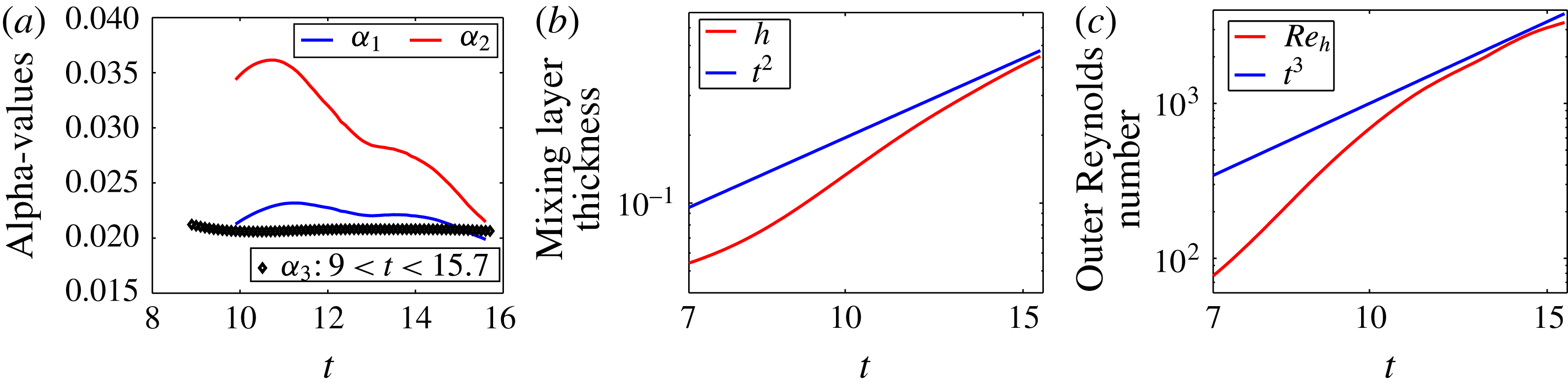
was also independently derived by Cook et al. (Reference Cook, Cabot and Miller2004) and by Jacobs & Dalziel (Reference Jacobs and Dalziel2005). Results are displayed in figure 1(a). It turns out that the first two evaluations depend strongly on time, while the third gives close results depending on the time range used. The value
 $\unicode[STIX]{x1D6FC}_{b3}=0.021$
, obtained from a fit performed in the time interval
 $9\leqslant t\leqslant 15.7$
, is retained. This value is at the lower bound of the admitted range (Glimm et al.
Reference Glimm, Sharp, Kaman and Lim2013; Youngs Reference Youngs2013). Figure 1(b) displays the mixing layer thickness calculated from
 $h(t)=3\langle \overline{c}(1-\overline{c})\rangle$
, as suggested by Poujade & Peybernes (Reference Poujade and Peybernes2010). It shows a good agreement with the
 $t^{2}$
-power law at the end of the calculation. The evolution of the outer Reynolds number
 $\mathit{Re}_{h}=4\mathit{Re}h{\dot{h}}$
, compared with the
 $t^{3}$
-power law is also shown (figure 1
c). The horizontal and vertical Taylor Reynolds numbers are
 $\mathit{Re}_{\unicode[STIX]{x1D706}_{xx}}=\mathit{Re}\unicode[STIX]{x1D706}_{xx}\sqrt{2\widetilde{k}}\approx 86$
and
 $\mathit{Re}_{\unicode[STIX]{x1D706}_{zz}}=\mathit{Re}\unicode[STIX]{x1D706}_{zz}\sqrt{2\widetilde{k}}\approx 142$
, respectively. This set of global quantities shows that the simulation satisfies the classical quality criteria, i.e. the
 $\unicode[STIX]{x1D6FC}_{b}$
coefficient, the evolution of the mixing length,
 $h(t)$
and the Reynolds number evolutions,
 $\mathit{Re}_{h}$
and
 $\mathit{Re}_{\unicode[STIX]{x1D706}_{zz}}$
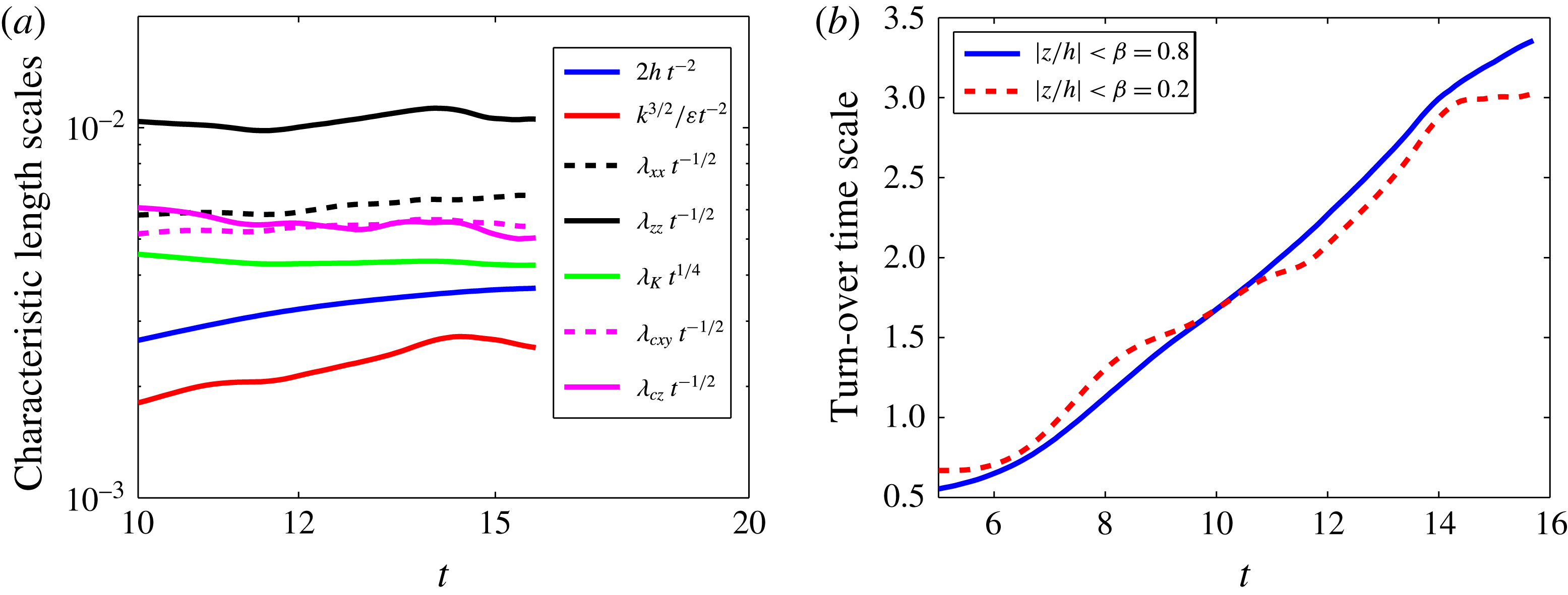
. Prior to a data analysis, it is also useful to draw the main characteristic length scales. The evolution of the following length scales are plotted in figure 2(a):
(a) The three methods to evaluate the
 $\unicode[STIX]{x1D6FC}_{b}$
-constant; evolution of
 $\unicode[STIX]{x1D6FC}_{b1}$
,
 $\unicode[STIX]{x1D6FC}_{b2}$
and
 $\unicode[STIX]{x1D6FC}_{b3}$
versus time (blue, red and black lines, respectively). The value
 $\unicode[STIX]{x1D6FC}_{b}=0.021$
is retained. (b) Mixing layer thickness calculated from
 $h(t)=3\langle \overline{c}(1-\overline{c})\rangle$
(red) with the
 $t^{2}$
-power law (blue). (c) Outer Reynolds number
 $\mathit{Re}_{h}=4\mathit{Re}h{\dot{h}}$
(red), with the
 $t^{3}$
-power law (blue).

-
(i) mixing zone thickness
 $\mathscr{L}=2h$
;
-
(ii) integral scale
$\ell =\langle \overline{k}_{B}^{3/2}/\overline{\unicode[STIX]{x1D700}}\rangle _{\unicode[STIX]{x1D6FD}}$
; -
(iii) horizontal Taylor length scale,
$\unicode[STIX]{x1D706}_{xx}^{2}=\langle \overline{u_{x}^{\prime 2}}/\overline{(\unicode[STIX]{x2202}_{x}u_{x}^{\prime })^{2}}\rangle _{\unicode[STIX]{x1D6FD}}$
; -
(iv) vertical Taylor length scale,
$\unicode[STIX]{x1D706}_{zz}^{2}=\langle \overline{u_{z}^{\prime 2}}/\overline{(\unicode[STIX]{x2202}_{z}u_{z}^{\prime })^{2}}\rangle _{\unicode[STIX]{x1D6FD}}$
; -
(v) horizontal Taylor mixing length scale,
$\unicode[STIX]{x1D706}_{cxy}^{2}=2\;\langle \overline{c^{\prime 2}}/(\overline{(\unicode[STIX]{x2202}_{x}c^{\prime })^{2}}+\overline{(\unicode[STIX]{x2202}_{y}c^{\prime })^{2}})\rangle _{\unicode[STIX]{x1D6FD}}$
; -
(vi) vertical Taylor mixing length scale,
$\unicode[STIX]{x1D706}_{cz}^{2}=\langle \overline{c^{\prime 2}}/\overline{(\unicode[STIX]{x2202}_{z}c^{\prime })^{2}}\rangle _{\unicode[STIX]{x1D6FD}}$
; -
(vii) Kolmogorov length scale,
$\unicode[STIX]{x1D706}_{K}=(\mathit{Re}^{3}\langle \overline{\unicode[STIX]{x1D700}}\rangle _{\unicode[STIX]{x1D6FD}})^{-1/4}$
;







with
 $\unicode[STIX]{x1D6FD}=0.2$
. These length scales have been compensated by their temporal scalings recalled in the introduction. The KO length scale is compensated by
 $t^{-1/4}$
, while the four Taylor length scales are compensated by
 $t^{1/2}$
. The integral scale
 $\ell$
and the largest length scale
 $\mathscr{L}=2h$
are both compensated by
 $t^{2}$
. This shows how the various steps of the evolution of the flow (transition to turbulence and to self-similarity) are reached, at different scales. It appears that the integral length scale is not stabilized, the thickness is converging, while the horizontal length scales
 $\unicode[STIX]{x1D706}_{xx}$
and
 $\unicode[STIX]{x1D706}_{cxy}$
have almost reached their temporal scalings. The vertical length scales
 $\unicode[STIX]{x1D706}_{zz}$
and
 $\unicode[STIX]{x1D706}_{cz}$
reach their scalings around
 $t\approx 15$
. The Kolmogorov scale, i.e. the smallest scale, reaches its temporal scaling very early, at around
 $t\approx 12$
. As a result the RT-turbulence spectrum widens both at low wavenumbers, as
 $t^{-2}$
, and large wavenumbers, as
 $t^{+1/4}$
. Finally, the chronology of the simulation is the following. The linear regime ends very early and mushroom-like structures appear visually at time
 $t\approx 5.5$
, transition to turbulence occurs at
 $t\approx 8.5$
, where a plateau has been reached for the ratio of the integral scale to the mixing zone thickness
 $\ell /\mathscr{L}\approx 0.7$
. Transition to self-similarity occurs at
 $t\approx 11$
. This estimate is based on the evolution of the outer Reynolds number
 $\mathit{Re}_{h}$
. Finally the simulation has been stopped at
 $t=15.7$
, where only few large-scale bubbles are present (figure 22). The evolution of the turn-over time scale
 $\langle \overline{k}_{B}/\overline{\unicode[STIX]{x1D700}}\rangle _{\unicode[STIX]{x1D6FD}}$
is displayed in figure 2(b), with
 $\unicode[STIX]{x1D6FD}=0.8$
and
 $0.2$
. It turns out that this time scale reaches a plateau at
 $t\approx 14$
in the very central part of the layer.
(a) Characteristic length scales versus time. The KO length scale
 $\unicode[STIX]{x1D706}_{K}$
compensated by
 $t^{-1/4}$
; the vertical Taylor mixing length scale
 $\unicode[STIX]{x1D706}_{cz}$
, the horizontal Taylor mixing length scale
 $\unicode[STIX]{x1D706}_{cxy}$
, the horizontal Taylor length scale
 $\unicode[STIX]{x1D706}_{xx}$
, the vertical Taylor length scale
 $\unicode[STIX]{x1D706}_{zz}$
, all four Taylor scales being compensated by
 $t^{1/2}$
; the integral scale
 $\ell$
and the largest length scale
 $\mathscr{L}=2h$
both compensated by
 $t^{2}$
. (b) Turn-over time scale versus time,
 $\langle \overline{k}_{B}/\overline{\unicode[STIX]{x1D700}}\rangle _{\unicode[STIX]{x1D6FD}}$
, with
 $\unicode[STIX]{x1D6FD}=0.8$
and 0.2.

Times
 $t=12.4$
and 15.7 are often used in the data analysis given below. They correspond to a time where the flow is turbulent and in a quasi-self-similar regime and to the final time of the simulation, where the flow is more turbulent and in a more achieved self-similar regime.
4 Velocity, pressure, kinetic energy and dissipation
4.1 Velocity
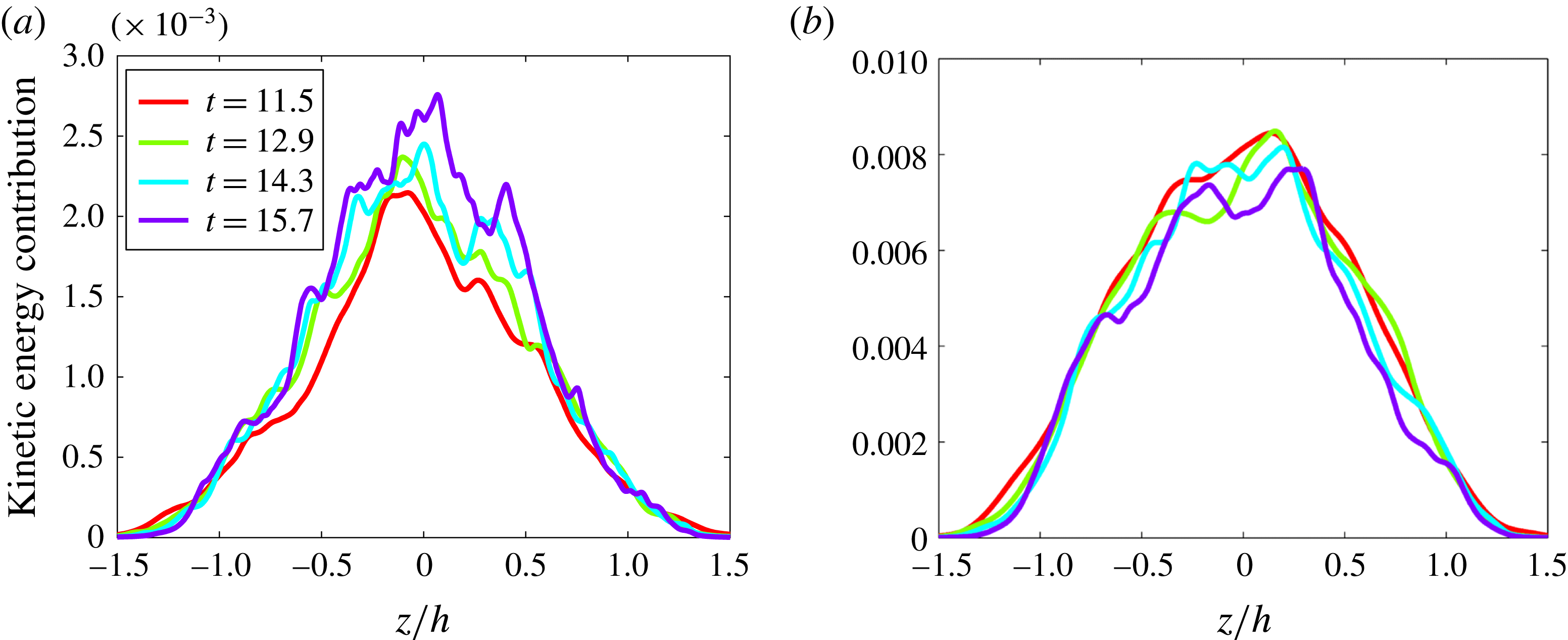
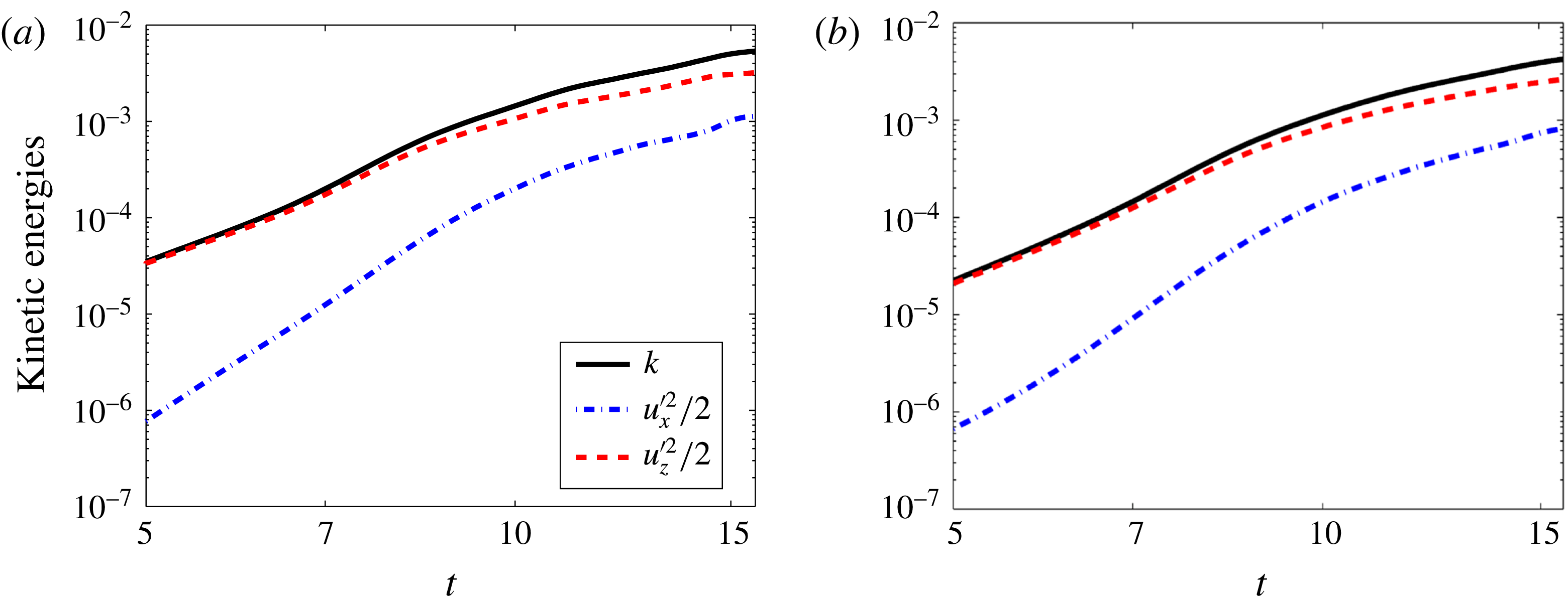
The self-similar character of the Boussinesq turbulence has been investigated in detail in Ristorcelli & Clark (Reference Ristorcelli and Clark2004). In particular, scalings of various quantities have emerged from this analysis. These scalings are used below to check the self-similarity of the flow. Figure 3 displays the superimposition of velocity moments
 $\overline{u_{x,z}^{\prime 2}}/2h$
(contributions to the kinetic energy) versus the self-similar variable
 $z/h$
. A trend to convergence is observed for the horizontal contribution, while it is clearly confirmed for the vertical contribution. Figure 4 confirms this trend. Note that the velocity profile supports are larger than the mixing layer thickness. These velocities correspond to large-scale bubbles escaped from the mixing layer and located beyond the front defined by
 $h(t)$
.
Velocity fluctuation kinetic energy versus the self-similar coordinate
 $z/h$
at four different times
 $t=11.5$
,
 $t=12.9$
,
 $t=14.3$
and
 $t=15.7$
. (a) Horizontal velocity component
 $\overline{u_{x}^{\prime 2}}/2h$
. (b) Vertical velocity
 $\overline{u_{z}^{\prime 2}}/2h$
. The trend to convergence of the latter appears clearly.

Velocity fluctuation kinetic energies,
 $\langle \overline{k}\rangle _{\unicode[STIX]{x1D6FD}}$
(black),
 $\langle \overline{u_{x}^{\prime 2}}\rangle _{\unicode[STIX]{x1D6FD}}/2$
(blue) and
 $\langle \overline{u_{z}^{\prime 2}}\rangle _{\unicode[STIX]{x1D6FD}}/2$
(red), versus time in log–log scale. Beginning of convergence is more pronounced for the vertical contribution. Two values of
 $\unicode[STIX]{x1D6FD}$
,
 $\unicode[STIX]{x1D6FD}=0.2$
(a) and 0.8 (b). The result does not depend significantly on this value.

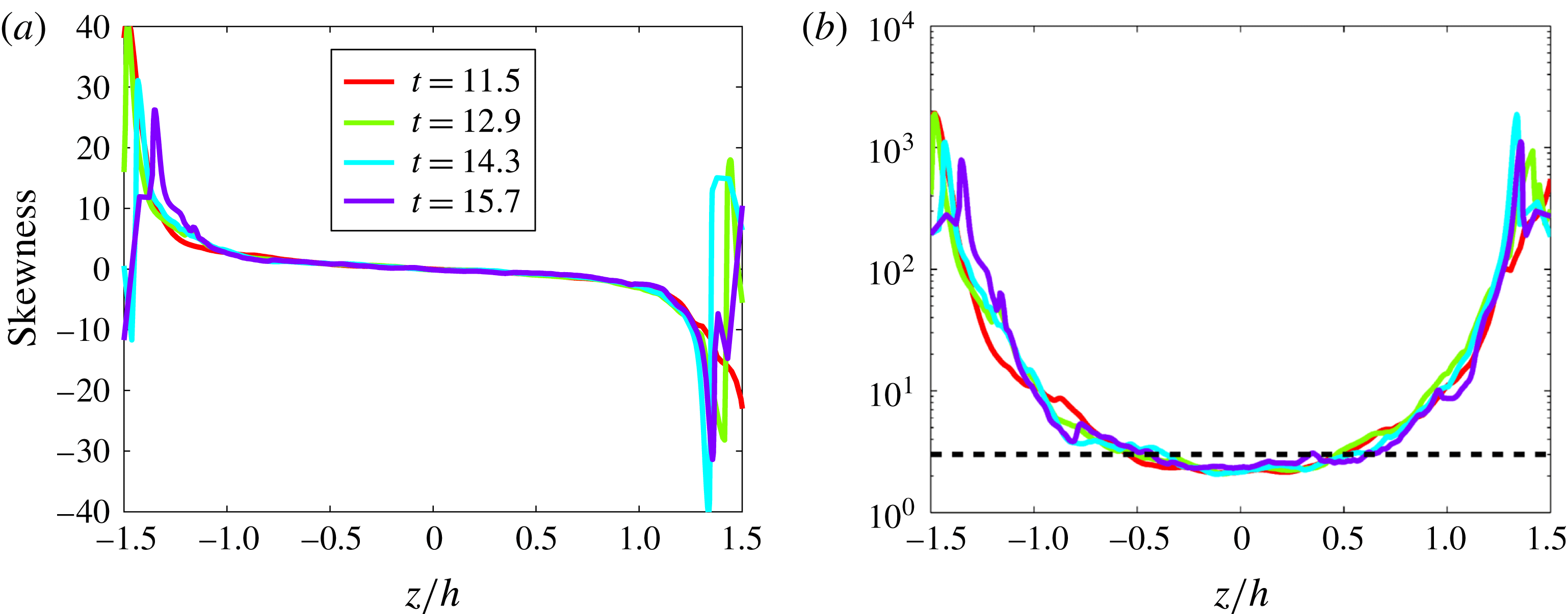
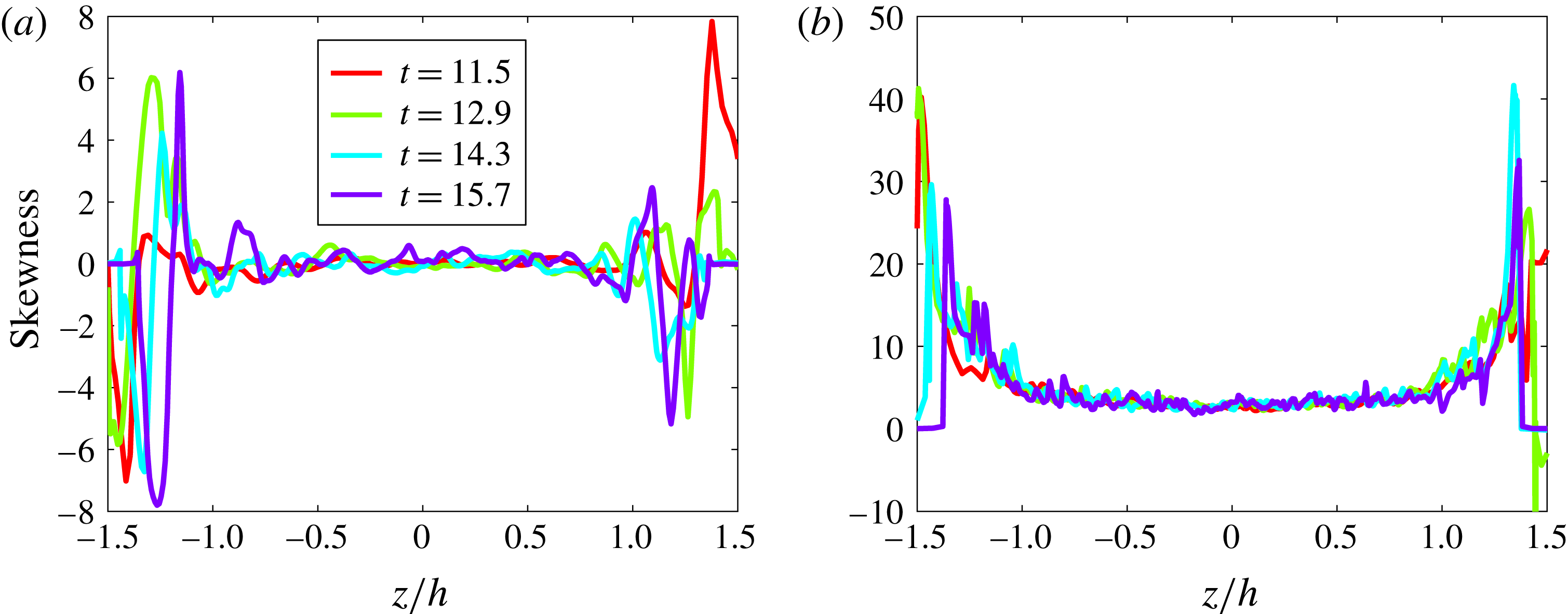
The velocity statistics are now described. The skewness of one horizontal velocity component,
 $\overline{u_{x}^{\prime 3}}/\overline{u_{x}^{\prime 2}}^{3/2}$
and the vertical component,
 $\overline{u_{z}^{\prime 3}}/\overline{u_{z}^{\prime 2}}^{3/2}$
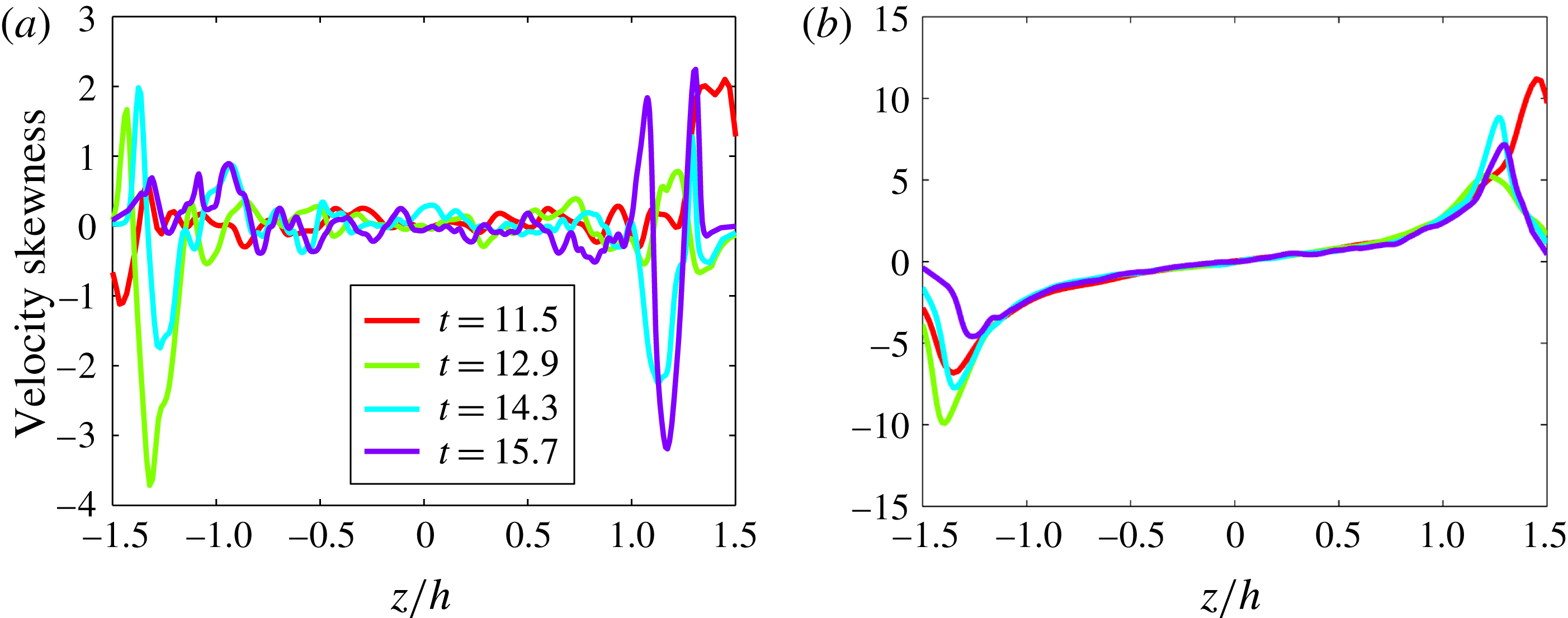
, are represented in figure 5. Skewness measures the asymmetry of the PDF of the corresponding quantity. For the
 $x$
component, the skewness has no particular structure. Very small values are obtained in the middle of the mixing layer and large values are obtained on the mixing layer boundaries. We may thus anticipate symmetric velocity component PDFs. Recall that the Reynolds number reaches its maximum at the centre of the mixing layer and decreases sharply at the boundaries. The skewness of the
 $z$
-velocity component is made of two peaks roughly centred around
 $z/h=\pm 1.4$
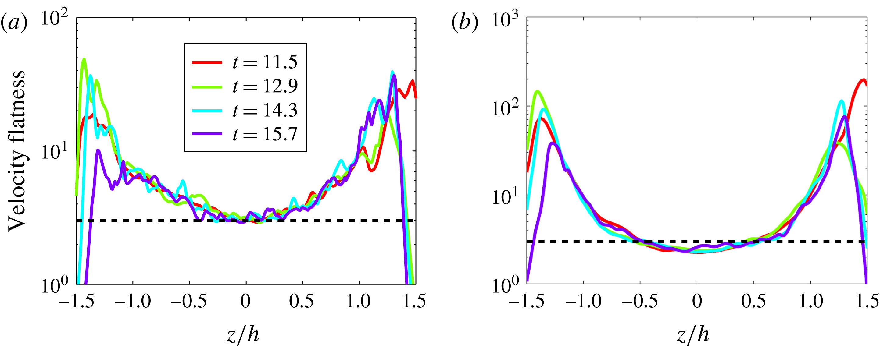
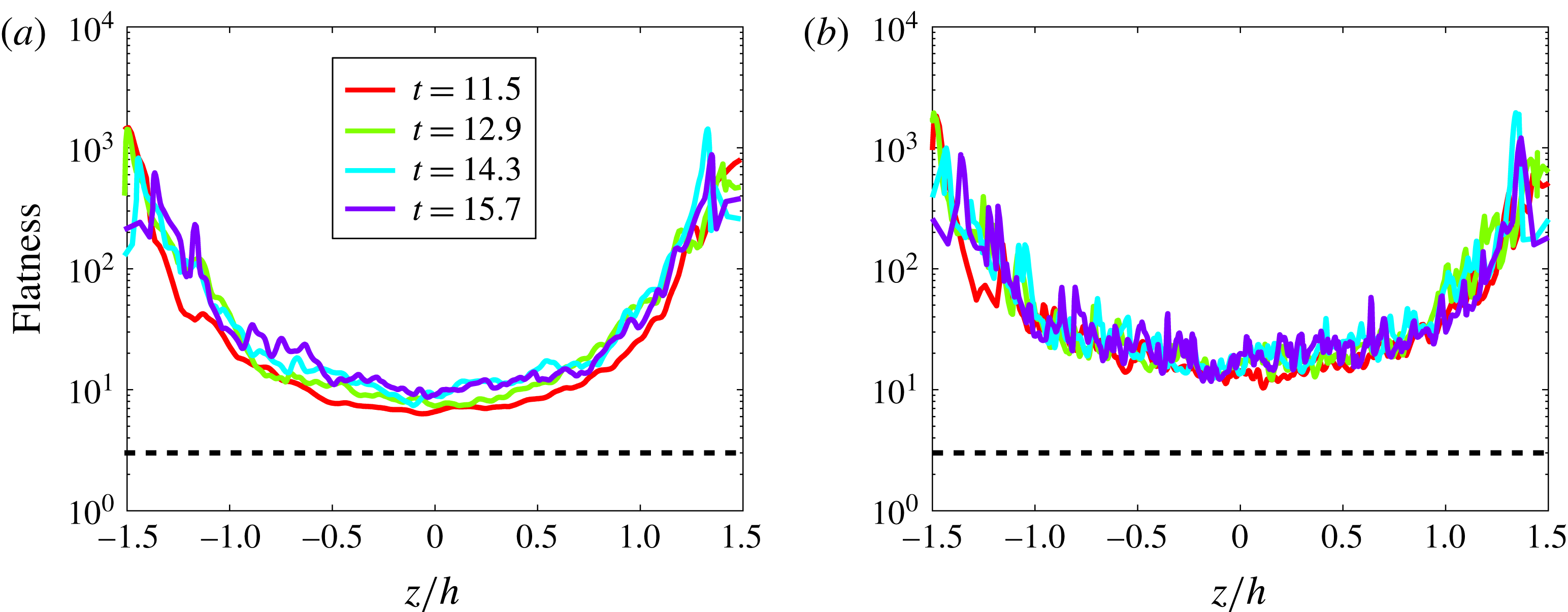
, corresponding to the mixing layer boundaries, matched by a region of small values. Peaks have the sign of the predominant events, i.e. positive velocities on the upper side and negative on the lower side. Flatness of the two velocity components are given in figure 6. Once again, flatnesses have peaks corresponding to the mixing layer boundaries. However inside the mixing layer flatnesses are close to 3, the value of a Gaussian random process.
Skewness of the velocity fluctuations versus the self-similar coordinate
 $z/h$
at four different times
 $t=11.5$
,
 $t=12.9$
,
 $t=14.3$
and
 $t=15.7$
. (a) Horizontal velocity component
 $\overline{u_{x}^{\prime 3}}/\overline{u_{x}^{\prime 2}}^{3/2}$
. (b) Vertical velocity
 $\overline{u_{z}^{\prime 3}}/\overline{u_{z}^{\prime 2}}^{3/2}$
.

Flatness of the velocity fluctuations versus the self-similar coordinate
 $z/h$
at four different times
 $t=11.5$
,
 $t=12.9$
,
 $t=14.3$
and
 $t=15.7$
. (a) Horizontal velocity component
 $\overline{u_{x}^{\prime 4}}/\overline{u_{x}^{\prime 2}}^{2}$
. (b) Vertical velocity
 $\overline{u_{z}^{\prime 4}}/\overline{u_{z}^{\prime 2}}^{2}$
. The flatness of a Gaussian process is represented by the horizontal dashed line.

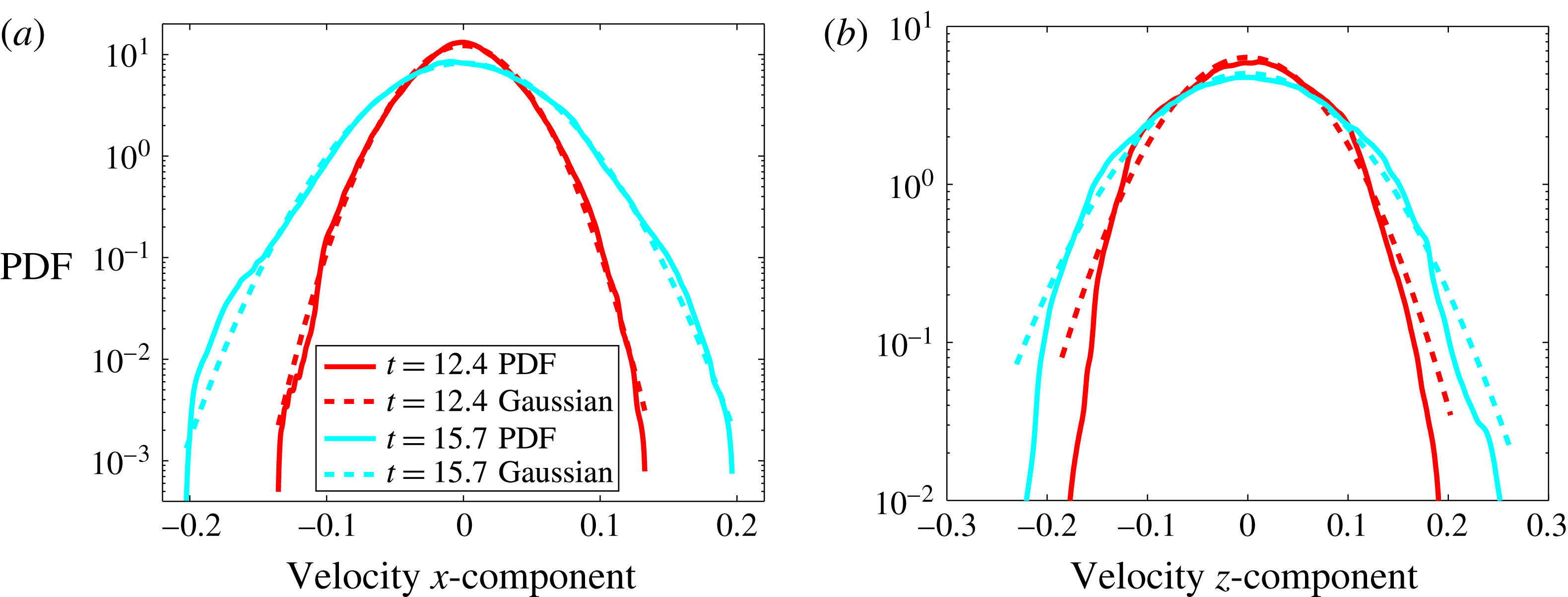
PDFs of the velocity components,
 $u_{x}^{\prime }$
(a) and
 $u_{z}^{\prime }$
(b). PDFs have been built with data located in the domain
 $[0:1;0:1;z_{1}:z_{2}]$
, where
 $z_{1}$
and
 $z_{2}$
are defined by
 $\overline{c}(z_{1})=0.4$
and
 $\overline{c}(z_{2})=0.6$
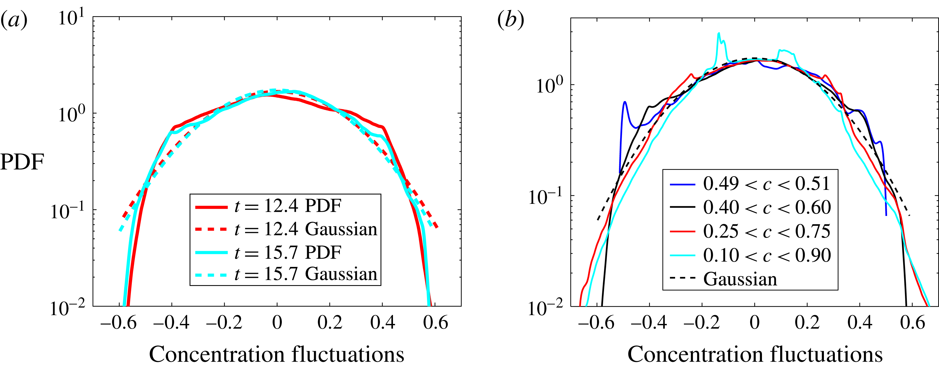
(see appendix B). On each plot, the dashed lines show Gaussian distribution with the same mean and variance.

These skewness and flatness plots have to be read with the velocity component PDFs represented in figure 7. It appears that the
 $x$
-velocity component PDF follows a Gaussian behaviour, even at the first selected time
 $t=12.4$
. Only small departures from Gaussianity is observed for large-amplitude events. This is mainly the case for the
 $z$
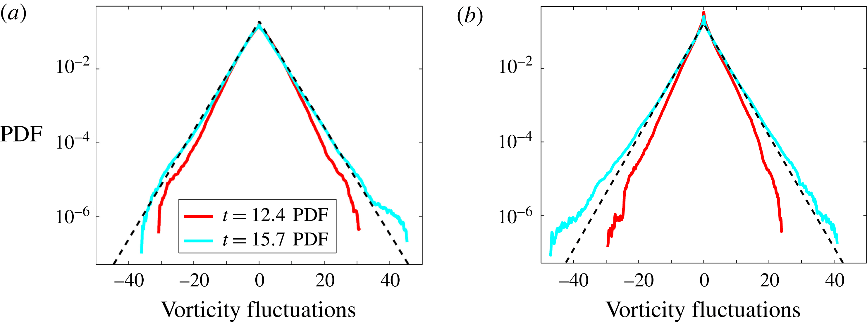
component. The Gaussian behaviour is associated with random interactions (She, Jackson & Orszag Reference She, Jackson and Orszag1990) and no particular structure is attached to this behaviour. However, velocity data located around the boundaries, which are not turbulent, have been excluded. We will see in § 5 that this Gaussian behaviour does not hold for vorticity, i.e. for the velocity gradients.
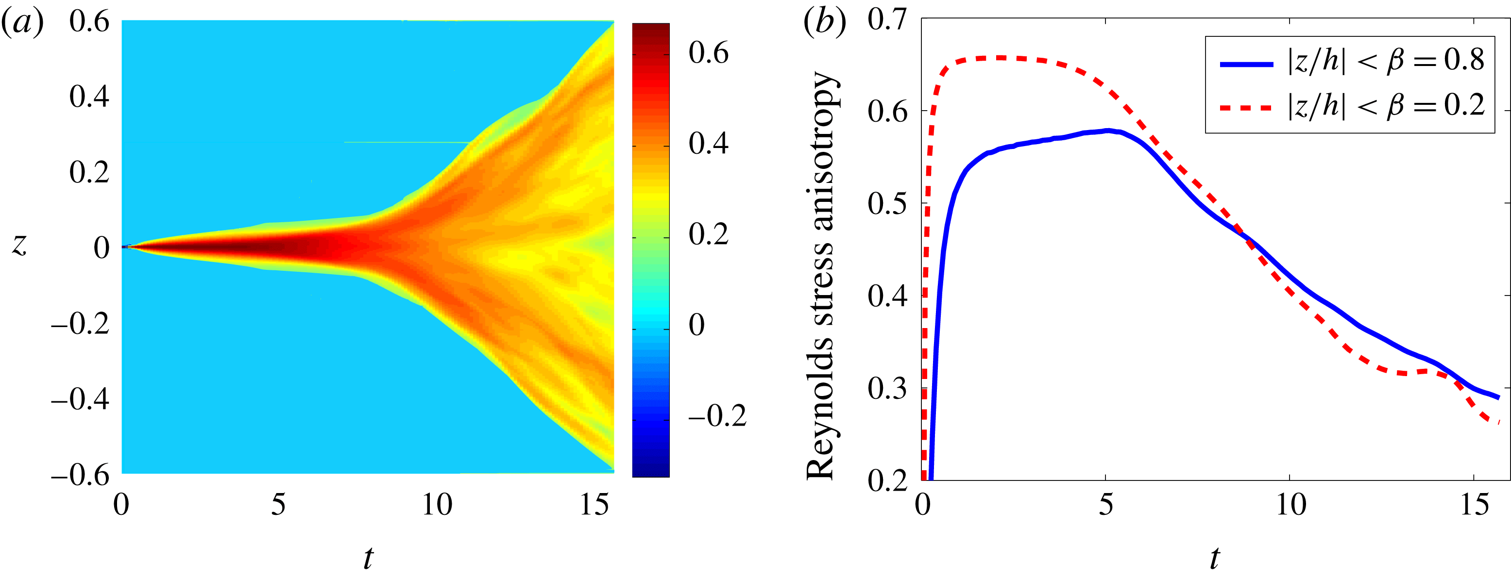
Reynolds stress anisotropy tensor. (a) 2-D map in the plane
 $(t,z)$
of the component
 $\overline{\unicode[STIX]{x1D623}}_{zz}$
. (b) Evolution of the averaged value,
 $\langle \overline{\unicode[STIX]{x1D623}}_{zz}\rangle _{\unicode[STIX]{x1D6FD}}$
versus time. Two values of
 $\unicode[STIX]{x1D6FD}$
have been used, 0.2 (red line) and 0.8 (blue line).

Since anisotropy at various scales is an issue of RT-Boussinesq turbulence, we investigate this issue with three indicators. First, turbulence anisotropy is classically measured with the Reynolds stress anisotropy tensor
 $$\begin{eqnarray}\displaystyle \overline{\unicode[STIX]{x1D623}}_{ij}=\displaystyle \frac{\overline{u_{i}^{\prime }u_{j}^{\prime }}}{2\overline{k}_{B}}-\displaystyle \frac{1}{3}\unicode[STIX]{x1D6FF}_{ij}\quad \text{for }i,j=1,2,3. & & \displaystyle\end{eqnarray}$$
This quantity is mainly related to the large scales. The behaviour of the third diagonal component
 $\unicode[STIX]{x1D623}_{zz}$
is reported in figure 8. The 2-D map of
 $\overline{\unicode[STIX]{x1D623}}_{zz}$
in the plane
 $(t,z)$
shows the inhomogeneity of the anisotropy in the
 $z$
-direction. However the evolution of the mean value
 $\langle \overline{\unicode[STIX]{x1D623}}_{zz}\rangle _{\unicode[STIX]{x1D6FD}}$
shows a trend to convergence. The anisotropy decrease is faster at the very middle of the layer (
 $\unicode[STIX]{x1D6FD}=0.2$
, red dashed line). This is in agreement with previous findings about large-scale anisotropy. Indeed Vladimirova & Chertkov (Reference Vladimirova and Chertkov2009) and Boffetta et al. (Reference Boffetta, Mazzino, Musacchio and Vozella2009) report an anisotropy between the two velocity components equal to
 $w_{rms}/u_{rms}\approx 1.8$
. Second velocity anisotropy at various scales may be investigated with the following indicator
 $$\begin{eqnarray}\displaystyle B_{\unicode[STIX]{x2202}_{k}^{(d)}u_{z}^{\prime }}=\left\langle \displaystyle \frac{\overline{(\unicode[STIX]{x2202}_{k}^{(d)}u_{z}^{\prime })^{2}}}{\overline{\unicode[STIX]{x2202}_{k}^{(d)}u_{i}^{\prime }\unicode[STIX]{x2202}_{k}^{(d)}u_{i}^{\prime }}}\right\rangle _{\unicode[STIX]{x1D6FD}}-\displaystyle \frac{1}{3}, & & \displaystyle\end{eqnarray}$$
with summation on the index
 $i$
, but not on
 $k=x,z$
. The superscript
 $(d)$
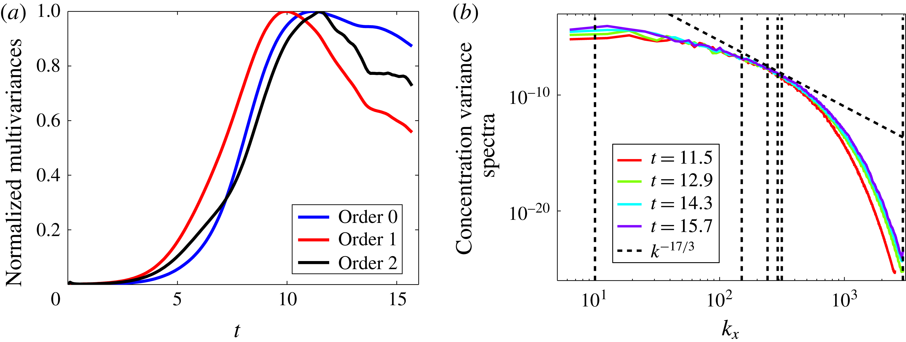
is the order of the derivative. Definition (4.2) generalizes the Reynolds stress tensor anisotropy (4.1) and gives some indications on the return to isotropy of the various scales, depending on the value of
 $d$
. For
 $d=0$
, one has
 $B_{\unicode[STIX]{x2202}_{k}^{(0)}u_{z}^{\prime }}\equiv b_{zz}$
, while for
 $d=1$
, this quantity may be seen as a measure of intermediate-scale anisotropy. For
 $d=2$
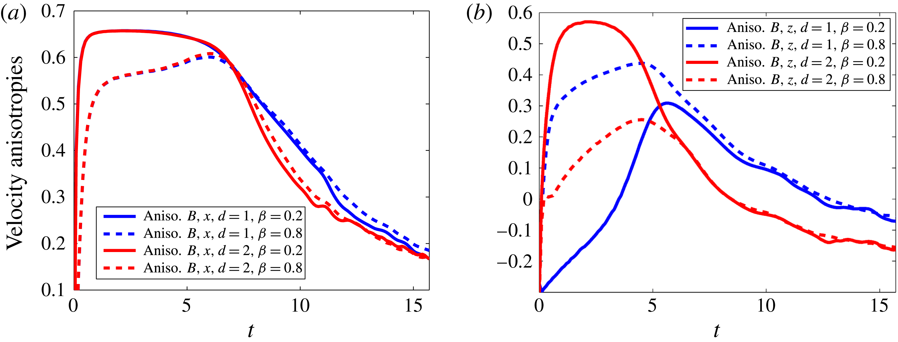
, it gives the small-scale anisotropy. Similar quantities have been introduced by Lin, Thiffeault & Doering (Reference Lin, Thiffeault and Doering2011) and called ‘multiscale variances’ in order to quantify the efficiency of mixing on different scales. The evolution of these indicators is given in figure 9. In figure 9(a), horizontal gradient evolution is shown. First- and second-order derivatives roughly behave in the same way. During the nonlinear regime,
 $t\leqslant 5.5$
, the indicator
 $B$
reaches large values, approximately 0.6, so that the horizontal gradients of the vertical velocity are much larger than the horizontal gradients of the horizontal velocities. This is related to the mainly vertical motions (updrafts and downdrafts) of the mushroom-like structures. Anisotropy decays slowly during the regime of transition to turbulence. At the end of the simulation, in the horizontal direction, intermediate and small scales have roughly the same ratio of anisotropy,
 $B_{\unicode[STIX]{x2202}_{x}^{(1)}u_{z}^{\prime }}\approx B_{\unicode[STIX]{x2202}_{x}^{(2)}u_{z}^{\prime }}\approx 0.20$
, so that the horizontal gradients of the vertical velocity are around twice those of the horizontal velocities. In other words, a positive anisotropy means that
 $u_{z}^{\prime }$
-intermediate and small scales are stronger than the horizontal components. The specific value of
 $\unicode[STIX]{x1D6FD}$
is not essential. The situation is different in the vertical direction (figure 9
b), where anisotropies depend significantly on the value of
 $\unicode[STIX]{x1D6FD}$
. The indicator
 $B_{\unicode[STIX]{x2202}_{z}^{(1)}u_{z}^{\prime }}$
starts at approximately
 $-1/3$
, so that the vertical gradient of the vertical velocity is close to zero. It thus grows to approximately
 $1/3$
in the nonlinear regime. This means that the vertical gradient of the vertical velocity is roughly twice the same gradient of the horizontal velocity. However, for
 $\unicode[STIX]{x1D6FD}=0.8$
, the averaging partially encompasses the boundaries and anisotropy is therefore much larger. In the transitional regime, this difference vanishes, the anisotropy does not depend on
 $\unicode[STIX]{x1D6FD}$
. At the end of the simulation, anisotropies are both slightly negative. At intermediate scales, one has
 $B_{\unicode[STIX]{x2202}_{z}^{(1)}u_{z}^{\prime }}\approx -0.06$
, while at small scales
 $B_{\unicode[STIX]{x2202}_{z}^{(2)}u_{z}^{\prime }}\approx -0.15$
. It turns out that, at small scales,
 $u_{z}^{\prime }$
is smaller than the fluctuations in the horizontal directions.
Velocity anisotropies calculated from
 $B_{\unicode[STIX]{x2202}_{k}^{(d)}u_{z}^{\prime }}$
(definition (4.2)). (a) Intermediate-scale anisotropy
 $B_{\unicode[STIX]{x2202}_{x}^{(1)}u_{z}^{\prime }}$
(blue) and small-scale anisotropy
 $B_{\unicode[STIX]{x2202}_{x}^{(2)}u_{z}^{\prime }}$
(red). (b) Intermediate-scale anisotropy
 $B_{\unicode[STIX]{x2202}_{z}^{(1)}u_{z}^{\prime }}$
(blue) and small-scale anisotropy
 $B_{\unicode[STIX]{x2202}_{z}^{(2)}u_{z}^{\prime }}$
(red). The return to isotropy is quicker for the intermediate vertical scales. Two values of
 $\unicode[STIX]{x1D6FD}$
have been used, 0.2 (full lines) and 0.8 (dashed lines).

Velocity anisotropies calculated from
 $C_{\unicode[STIX]{x2202}_{z}^{(d)}u_{i}^{\prime }}$
(definition (4.3)). (a) Intermediate-scale anisotropy
 $C_{\unicode[STIX]{x2202}_{z}^{(1)}u_{x}^{\prime }}$
(blue) and small-scale anisotropy
 $C_{\unicode[STIX]{x2202}_{z}^{(1)}u_{z}^{\prime }}$
(red). (b) Intermediate-scale anisotropy
 $C_{\unicode[STIX]{x2202}_{z}^{(2)}u_{x}^{\prime }}$
(blue) and small-scale anisotropy
 $C_{\unicode[STIX]{x2202}_{z}^{(2)}u_{z}^{\prime }}$
(red). Two values of
 $\unicode[STIX]{x1D6FD}$
have been used, 0.2 (full lines) and 0.8 (dashed lines).

We use a third indicator to characterize the velocity anisotropy. We define
 $$\begin{eqnarray}\displaystyle C_{\unicode[STIX]{x2202}_{z}^{(d)}u_{i}^{\prime }}=\left\langle \displaystyle \frac{\overline{(\unicode[STIX]{x2202}_{z}^{(d)}u_{i}^{\prime })^{2}}}{\overline{|\unicode[STIX]{x1D735}^{(d)}u_{i}^{\prime }|^{2}}}\right\rangle _{\unicode[STIX]{x1D6FD}}-\displaystyle \frac{1}{3}. & & \displaystyle\end{eqnarray}$$
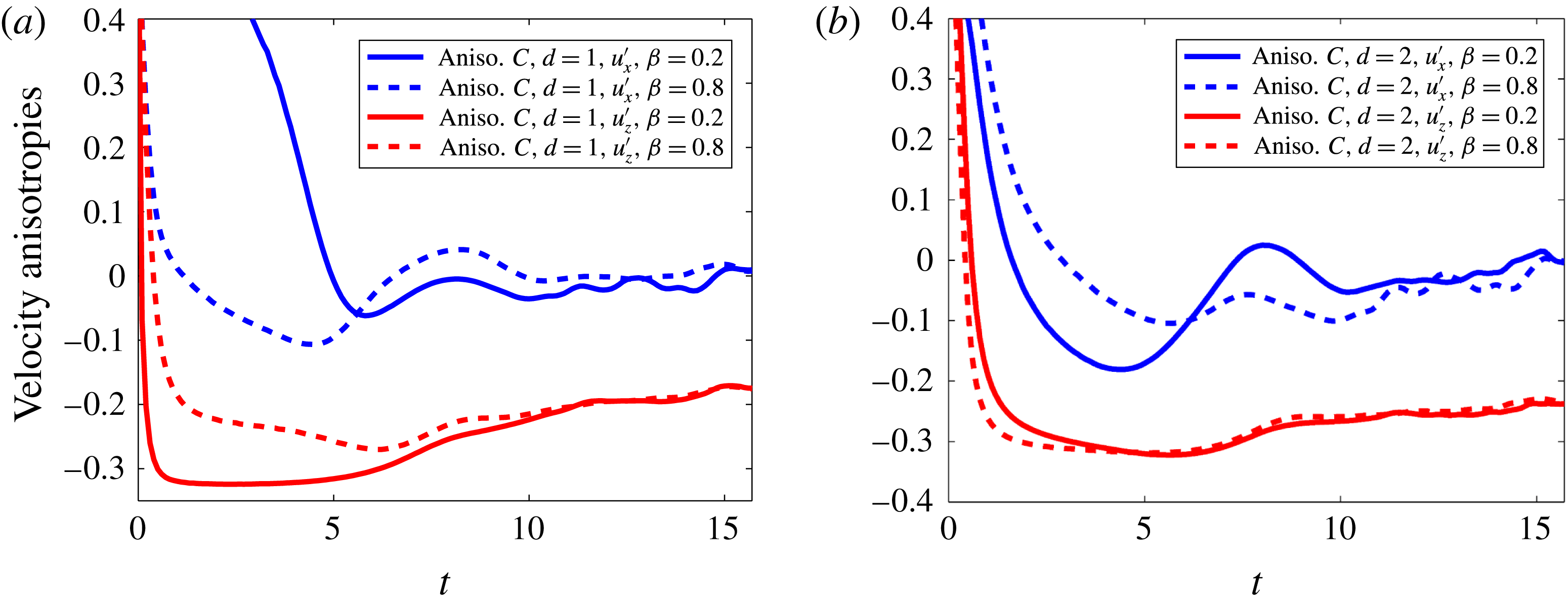
This definition applies to the three velocity components and it will allow us to compare with concentration anisotropies calculated in § 6 and displayed in figure 33. Criterion (4.3) is displayed in figure 10 for an horizontal and the vertical velocity component and for the intermediate (
 $d=1$
) and small (
 $d=2$
) scales. They all start with very large values and decay abruptly. At the beginning of the transitional regime they evolve slowly toward their final values. Within this transitional regime, the vertical gradient of the horizontal velocity reaches small values at the end of the transition for
 $\unicode[STIX]{x1D6FD}=0.8$
, while in the very interior of the mixing layer (
 $\unicode[STIX]{x1D6FD}=0.2$
) small anisotropy values are reached very early during the nonlinear regime. Vertical gradients of the vertical velocity are very small during the transitional regime and reach small negative values compatible with the quasi-isotropy of the intermediate scales. At the end of the simulation, it turns out that
 $C_{\unicode[STIX]{x2202}_{z}^{(1)}u_{x}^{\prime }}$
and
 $C_{\unicode[STIX]{x2202}_{z}^{(2)}u_{x}^{\prime }}$
goes to zero, while
 $C_{\unicode[STIX]{x2202}_{z}^{(1)}u_{z}^{\prime }}\approx -0.17$
and
 $C_{\unicode[STIX]{x2202}_{z}^{(2)}u_{z}^{\prime }}\approx -0.24$
. It means that with respect to the vertical gradient the horizontal velocity is almost isotropic but the vertical velocity component remains anisotropic both at intermediate and small scales. It is related to updraft and downdraft motions superimposed to the background turbulent flow. On the other hand, spectral velocity anisotropy have been investigated by Livescu et al. (Reference Livescu, Ristorcelli, Petersen and Gore2010) by taking the Fourier transform of the Reynolds stress anisotropy tensor,
 $\overline{\unicode[STIX]{x1D623}}_{zz}$
. We use here a fourth indicator, which will also be used for the concentration-gradient anisotropy
 $$\begin{eqnarray}\displaystyle S_{u}(k_{x},t)=\displaystyle \frac{\langle \widehat{u}_{3}^{2}(k_{x},k_{y}=0,z,t)\rangle }{\displaystyle \mathop{\sum }_{i=1}^{3}\langle \widehat{u}_{i}^{2}(k_{x},k_{y}=0,z,t)\rangle }-\displaystyle \frac{1}{3}, & & \displaystyle\end{eqnarray}$$
where
 $\widehat{u}$
denotes the Fourier transform of the variable
 $u$
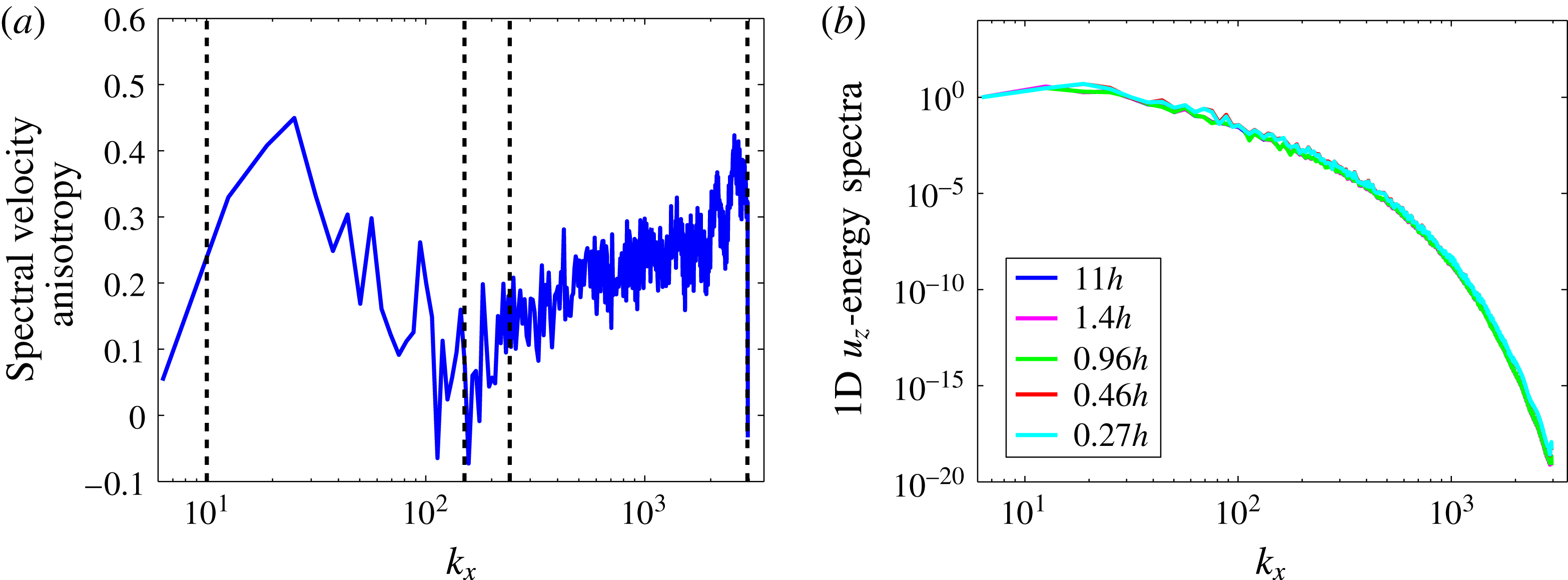
. The Fourier spectra calculation is detailed below. Results for velocity anisotropy are shown in figure 11(a), where the integral scale and the horizontal and vertical Taylor length scales have also been indicated. Anisotropy reaches very small values around these two length scales. For smaller scales, the anisotropy increases with the wavenumber
 $k_{x}$
up to the Kolmogorov length scale. It confirms that the intermediate velocity scales are nearly isotropic while small scales are anisotropic.
(a) Spectral anisotropy of the velocity field at the final time of the simulation. The vertical dashed black lines stand for the integral scale, the horizontal and vertical Taylor length scales and the Kolmogorov scale. (b) Spectra of the vertical velocity averaged over various heights in the vertical direction, from
 $0.27h$
to
 $11h$
. Spectra have been normalized by the first-mode amplitude. Final time of the simulation.

In this section and below, we show Fourier spectra of various quantities. In that purpose, spectra are computed by performing a 1-D Fourier transform in an horizontal direction and averaged with respect to the second horizontal direction. A vertical averaging is also performed. As a result, spectra depend on the horizontal wavenumber
 $k_{x}$
and on time
 $t$
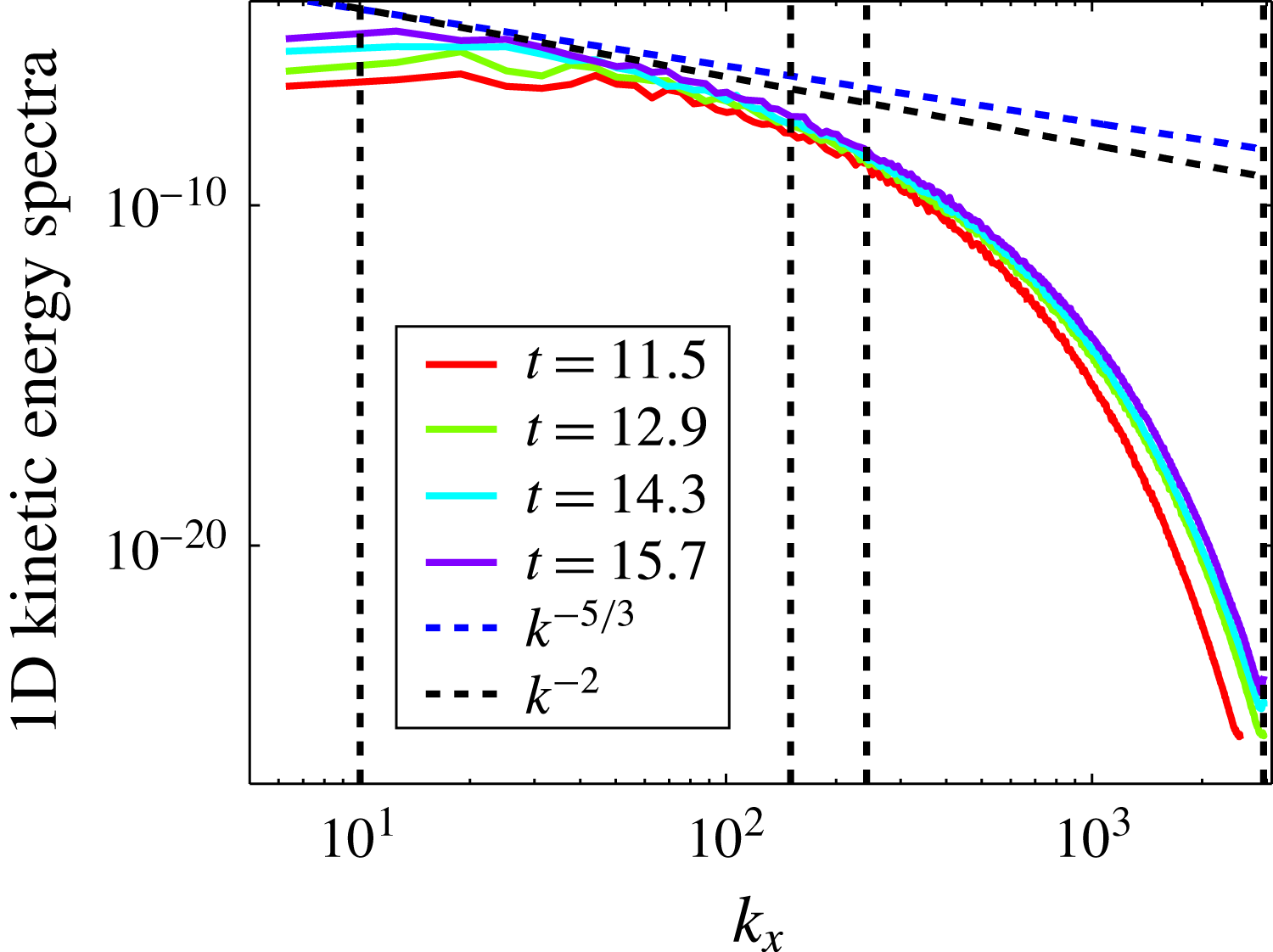
. The question arises of whether the result depends on the proportion of the mixing layer on which the average is performed. The answer is given in figure 11(b) where the spectra have been averaged on various fractions of the mixing layer. These spectra have also been normalized by the amplitude of the largest scale. It appears clearly that the spectral structure is invariant with respect to the vertical averaging. The 1-D energy spectra of the velocity fluctuations are presented in figure 12 at four different times. The two slopes,
 $k^{-5/3}$
and
 $k^{-2}$
, have also been displayed since the
 $k^{-2}$
energy spectrum has been suggested. However, LES and DNS seem to be in favour of the classical KO spectrum, at least within the Sandoval approximation (Cabot & Cook Reference Cabot and Cook2006; Livescu Reference Livescu2013). A short inertial range is visible between large and Taylor scales in figure 12, while a large dissipation zone is present. Since RT turbulence is continuously fed, spectra shift with time to higher energy. They also widen toward large scales on the one hand, and toward smaller scales on the other hand.
One-dimensional kinetic energy spectra as function of the wavenumber
 $k_{x}$
in a log–log scale. The vertical lines stand for the integral scale, the vertical and horizontal Taylor length scales and the Kolmogorov scale. Selected times are
 $t=11.5$
,
 $t=12.9$
,
 $t=14.3$
and
 $t=15.7$
.

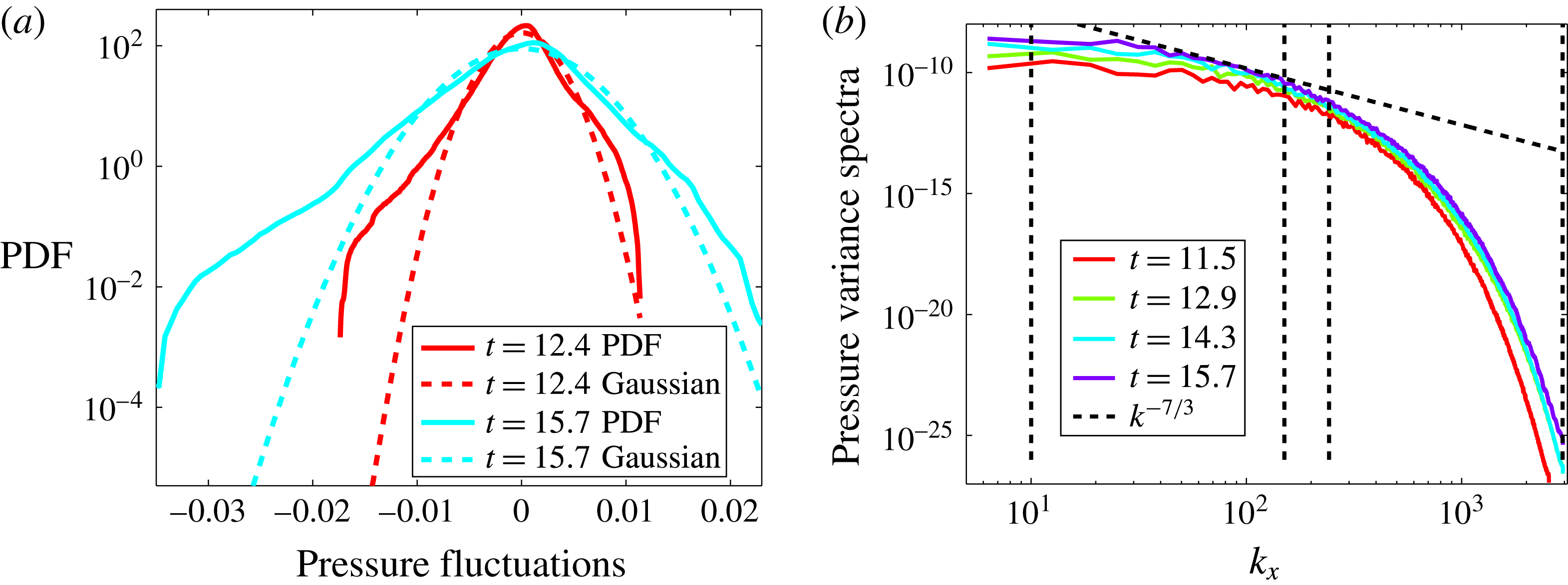
(a) PDF of the pressure fluctuations
 $p^{\prime }$
at two different times
 $t=12.4$
and
 $t=15.7$
. The corresponding Gaussian distributions are plotted in dashed lines. Departures from Gaussianity and asymmetry appear clearly. The PDFs have quasi-exponential wings in the lows and in the highs. However, negative values are more probable than positive values. This is related to the fact that centre of vortices correspond to pressure minima. (b) Power spectra of the pressure fluctuations at the four selected times
 $t=11.5$
,
 $t=12.9$
,
 $t=14.3$
and
 $t=15.7$
. The
 $k^{-7/3}$
-scaling has also been plotted. The vertical dashed lines have the same meaning as in figure 12.

The pressure PDFs have been plotted in figure 13(a) at two times,
 $t=12.4$
and
 $t=15.7$
. Departures from Gaussianity and asymmetry appear clearly on these plots. The positive side of the PDF behaves as an exponential. On the negative side, there are two different exponential regimes, which can also be approximated by straight lines of different slopes. This behaviour is consistent with earlier observations on various turbulent flows (Lesieur Reference Lesieur1997, § 8). Indeed, it occurs in decaying isotropic turbulence with Taylor–Green initial conditions (Brachet Reference Brachet1991). It also occurs in statistically steady turbulence (Pumir Reference Pumir1994a
; Cao, Chen & Doolen Reference Cao, Chen and Doolen1999) and it has been recently confirmed for the decaying isotropic turbulence (Kalelkar Reference Kalelkar2006). This asymmetry is related to the fact that centres of vortices correspond to pressure minima. Therefore high vorticity fluctuations are correlated with low pressure fluctuations. Moreover, it has been demonstrated by Pumir (Reference Pumir1994a
) that the superexponential part of the pressure PDF comes from intermittent fluctuations of vorticity. The pressure power spectra are displayed in figure 13(b). The
 $k^{-7/3}$
-scaling obtained from a quasi-normal approximation within an isotropic turbulence (Batchelor Reference Batchelor1971; Leslie Reference Leslie1973, § 11.5) is also plotted. This scaling appears to be a good fit for scales above the vertical Taylor length scale.
4.2 Mass flux spectrum
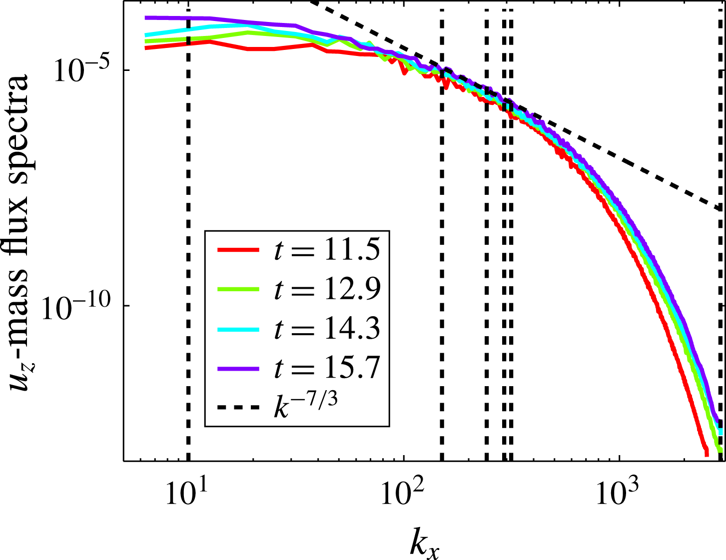
Figure 14 displays the spectra of the vertical mass flux
 $\unicode[STIX]{x1D70C}^{\prime }u_{z}^{\prime }$
at the four selected times. We have also plotted the
 $k^{-7/3}$
-scaling given by Lumley (Reference Lumley1967) to predict the effect of buoyancy on the turbulent energy spectrum (see also Kaneda & Yoshida (Reference Kaneda and Yoshida2004)). It provides a good scaling around the Taylor length scales.
One-dimensional spectra of the vertical component
 $\unicode[STIX]{x1D70C}^{\prime }u_{z}^{\prime }$
of the mass flux. The Lumley
 $k^{-7/3}$
-scaling has been plotted (dashed black line) and the vertical lines stand for the integral scale, the vertical and horizontal Taylor length scales, the horizontal and vertical Taylor mixing length scales and the Kolmogorov scale, respectively.

4.3 Dissipation
Dissipation is one of the key turbulent quantities that has to be investigated. It has been introduced in (2.22) and (2.23). In Ristorcelli & Clark (Reference Ristorcelli and Clark2004) it has been proved rigorously that the third dissipation component
 $\unicode[STIX]{x1D700}_{zz}$
scales as
 $h^{1/2}\propto t$
. Moreover, by dimensional analysis, it appears that the dissipation rate should grow linearly with time (Souffland et al.
Reference Souffland, Grégoire, Gauthier and Schiestel2002; Boffetta et al.
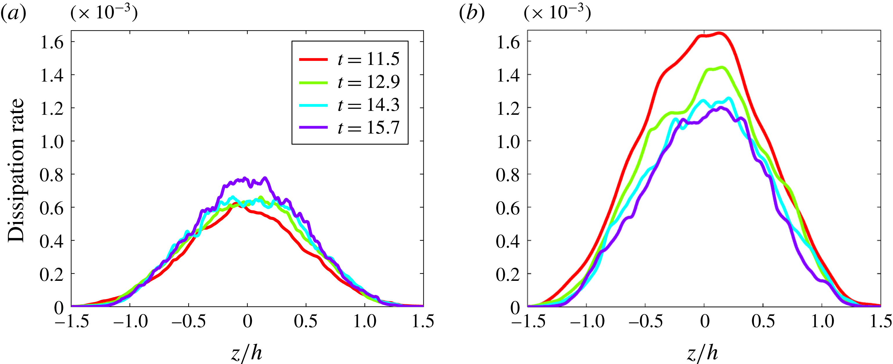
Reference Boffetta, Mazzino, Musacchio and Vozella2010). This scaling is used to check the self-similarity of the dissipation contributions. Figure 15 displays the
 $x$
(a) and
 $z$
(b)-contribution versus the self-similar variable, i.e.
 $\overline{\unicode[STIX]{x2202}_{j}u_{1}\unicode[STIX]{x2202}_{j}u_{1}}/h^{1/2}$
and
 $\overline{\unicode[STIX]{x2202}_{j}u_{3}\unicode[STIX]{x2202}_{j}u_{3}}/h^{1/2}$
versus
 $z/h$
. The
 $z$
-contribution is closer to convergence than the
 $x$
-contribution. On the other hand, if dissipation has reached a self-similar regime, one has
 $\overline{\unicode[STIX]{x1D700}}(z,t)=h^{1/2}(t)\unicode[STIX]{x1D6F6}(\unicode[STIX]{x1D709})$
, where
 $\unicode[STIX]{x1D6F6}$
is the structure function of the dissipation and
 $\unicode[STIX]{x1D709}=z/h(t)\sim z/t^{2}$
. In the self-similar regime, we must have
 $\int _{-\infty }^{+\infty }\unicode[STIX]{x1D6F6}(\unicode[STIX]{x1D709})\,\text{d}\unicode[STIX]{x1D709}=C^{st}$
. Therefore
 $$\begin{eqnarray}\displaystyle \int _{-\infty }^{+\infty }\overline{\unicode[STIX]{x1D700}}(z,t)\,\text{d}z\propto \int _{-\infty }^{+\infty }\overline{\unicode[STIX]{x1D700}}(z,t)t^{2}\,\text{d}\unicode[STIX]{x1D709}\propto t^{3}\int _{-\infty }^{+\infty }\unicode[STIX]{x1D6F6}(\unicode[STIX]{x1D709})\,\text{d}\unicode[STIX]{x1D709}\propto t^{3}. & & \displaystyle\end{eqnarray}$$
As a result, the
 $z$
-averaged value over the thickness
 $h(t)$
behaves as
 $$\begin{eqnarray}\displaystyle \langle \overline{\unicode[STIX]{x1D700}}\rangle =\displaystyle \frac{1}{h(t)}\int _{-\infty }^{+\infty }\overline{\unicode[STIX]{x1D700}}(z,t)\,\text{d}z\propto t. & & \displaystyle\end{eqnarray}$$
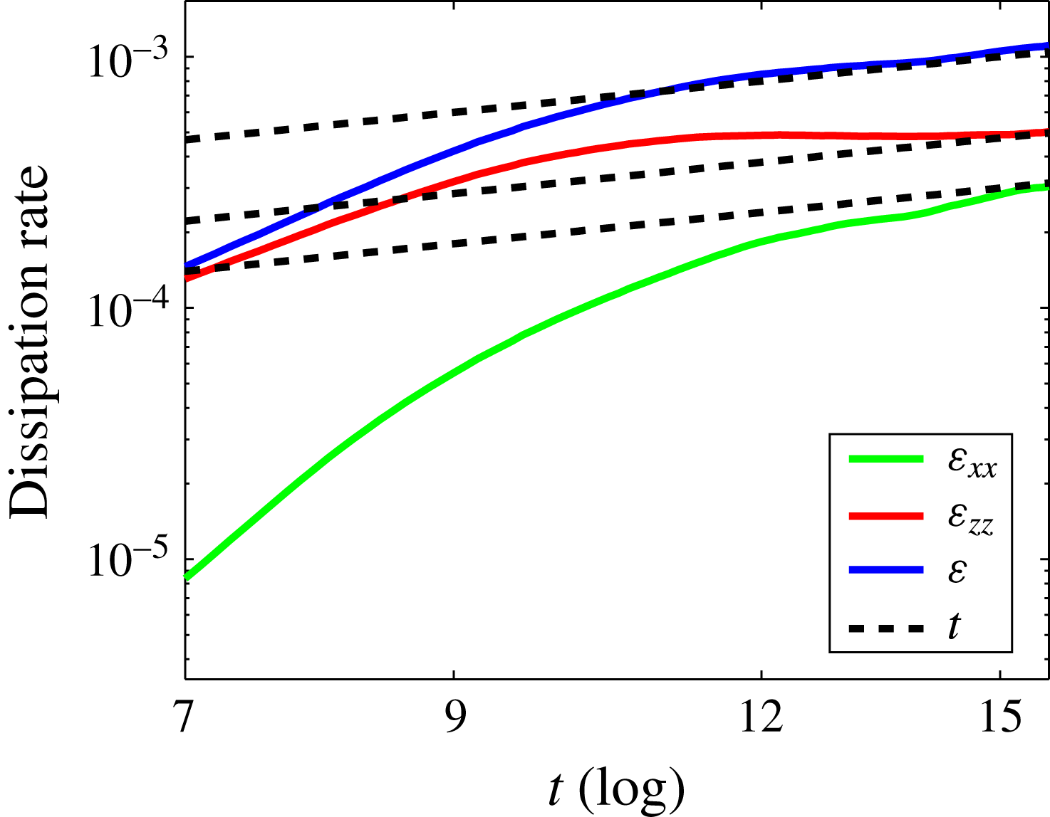
This result is well known in IHT (Sreenivasan Reference Sreenivasan1998). The evolution of the
 $x$
- and
 $z$
-contributions and the total dissipation rate is represented in figure 16. Both contributions show a satisfactory agreement with the linear temporal scaling (4.6) while the total dissipation rate displays a very good agreement.
Dissipation rate contributions
 $\unicode[STIX]{x1D700}_{jj}$
. (a) Scaled
 $x$
-contribution of the dissipation,
 $\overline{\unicode[STIX]{x2202}_{j}u_{1}\unicode[STIX]{x2202}_{j}u_{1}}/h^{1/2}$
, as a function of the self-similar variable
 $z/h$
for four different times. (b) Scaled
 $z$
-contribution of the dissipation,
 $\overline{\unicode[STIX]{x2202}_{j}u_{3}\unicode[STIX]{x2202}_{j}u_{3}}/h^{1/2}$
.

Dissipation rate
 $\unicode[STIX]{x1D700}$
. Evolution of the
 $x$
- and
 $z$
-contributions and the total dissipation, averaged over
 $xyz$
. The dissipation rate shows a very good agreement with the linear temporal scaling (4.6).

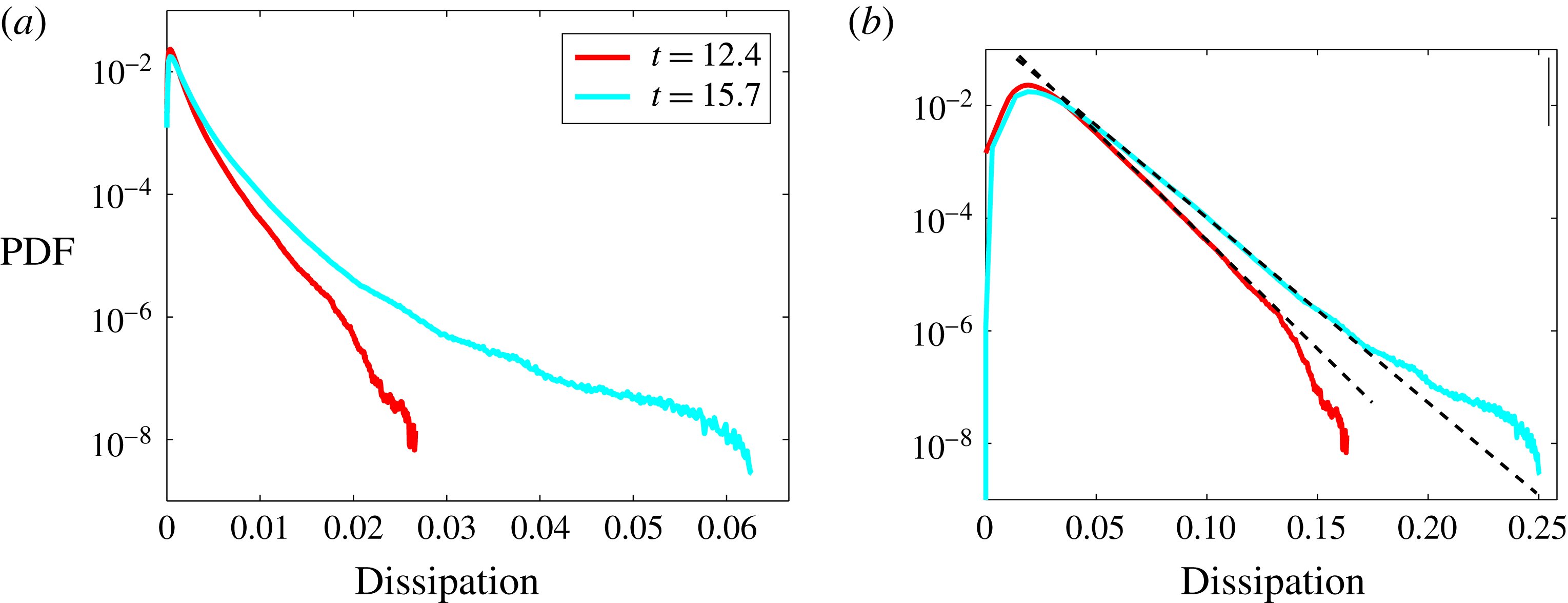
Finally, the PDF of the dissipation is displayed in figure 17 at two different times. Since dissipation is homogeneous to the square of a velocity gradient, we also display the PDF of the square-root of the dissipation
 $\unicode[STIX]{x1D700}$
. It clearly exhibits exponential wings. The slope increases with time – or the Reynolds number – and so does the intermittency.
PDF of the dissipation
 $\unicode[STIX]{x1D700}$
, at two different times. (a) PDF (
 $\unicode[STIX]{x1D700}$
). (b) PDF (
 $\unicode[STIX]{x1D700}^{1/2}$
), to highlight the exponential wings. The slope of these wings increases with time, i.e. the Reynolds number.

5 Vorticity
5.1 Vorticity properties
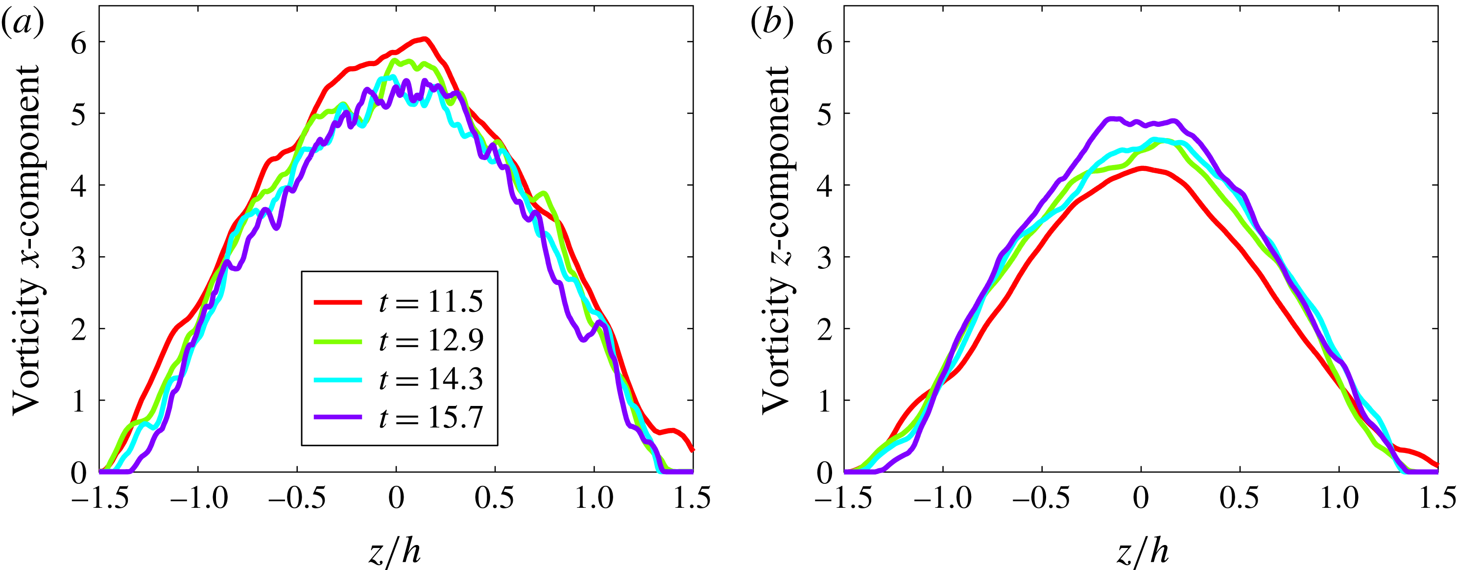
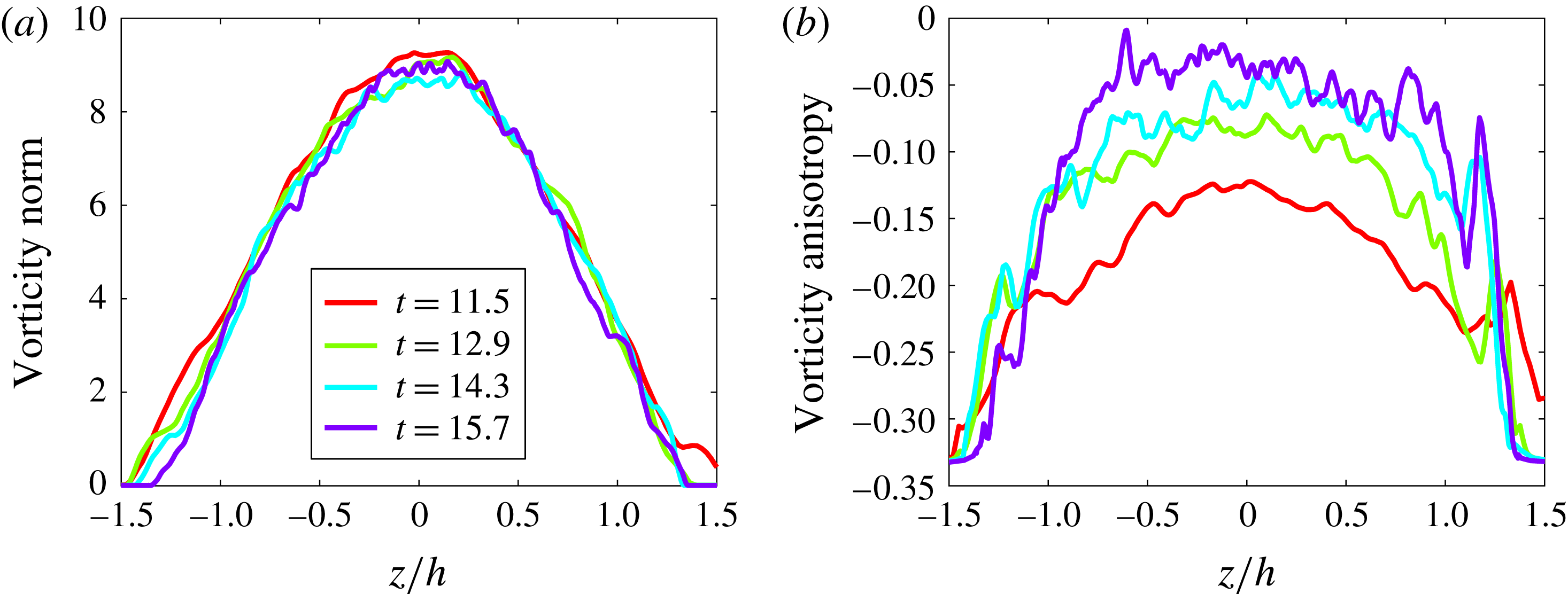
In this section we study the properties of the vorticity whose transport equation has been derived in § 2.3 for the RT-Boussinesq flow. On the one hand, the mean vorticity components are given by
 $$\begin{eqnarray}\displaystyle \overline{\unicode[STIX]{x1D714}}_{1}=-\unicode[STIX]{x2202}_{3}\overline{u}_{2},\quad \overline{\unicode[STIX]{x1D714}}_{2}=\unicode[STIX]{x2202}_{3}\overline{u}_{1}\quad \text{and}\quad \overline{\unicode[STIX]{x1D714}}_{3}=0. & & \displaystyle\end{eqnarray}$$
On the other hand, from the vorticity equation (2.21), one finds with the mean value definition (2.14)
 $$\begin{eqnarray}\displaystyle \left.\begin{array}{@{}c@{}}\displaystyle \unicode[STIX]{x2202}_{t}\overline{\unicode[STIX]{x1D714}}_{1}={\textstyle \frac{1}{2}}\overline{\unicode[STIX]{x1D714}_{3}^{\prime }\unicode[STIX]{x2202}_{3}u_{2}^{\prime }}+{\textstyle \frac{1}{2}}\overline{\unicode[STIX]{x1D714}_{3}^{\prime }\unicode[STIX]{x2202}_{1}u_{3}^{\prime }}+\unicode[STIX]{x2202}_{3}(-\overline{\unicode[STIX]{x1D714}_{1}^{\prime }u_{3}^{\prime }}+\mathit{Re}^{-1}\unicode[STIX]{x2202}_{3}\overline{\unicode[STIX]{x1D714}}_{1}),\\ \displaystyle \unicode[STIX]{x2202}_{t}\overline{\unicode[STIX]{x1D714}}_{2}={\textstyle \frac{1}{2}}\overline{\unicode[STIX]{x1D714}_{3}^{\prime }\unicode[STIX]{x2202}_{2}u_{3}^{\prime }}+{\textstyle \frac{1}{2}}\overline{\unicode[STIX]{x1D714}_{3}^{\prime }\unicode[STIX]{x2202}_{3}u_{2}^{\prime }}+\unicode[STIX]{x2202}_{3}(-\overline{\unicode[STIX]{x1D714}_{2}^{\prime }u_{3}^{\prime }}+\mathit{Re}^{-1}\unicode[STIX]{x2202}_{3}\overline{\unicode[STIX]{x1D714}}_{2}).\end{array}\right\} & & \displaystyle\end{eqnarray}$$
In these evolution equations, there is neither transport nor baroclinic production. The baroclinic term vanishes due to the symmetry of the RT-Boussinesq flow. Turbulence production is limited to the stretching contribution, i.e. production through correlation between the third vorticity component and the gradients of the horizontal velocity components. There are also two diffusion terms, one turbulent, one molecular. Moreover these non-zero mean vorticity values come from a small large-scale drift in the velocity field. As such, the averaged values of the vorticity components do not appear to be relevant to the understanding of vorticity motion. Let us note that such simplification does not occur in the compressible case where baroclinic contributions of the form
 $\unicode[STIX]{x1D700}_{ijk}\overline{\unicode[STIX]{x2202}_{j}\unicode[STIX]{x1D70C}^{\prime }\unicode[STIX]{x2202}_{k}p^{\prime }}$
do not vanish. We thus turn our attention to the square of the mean vorticity. Owing to vorticity equation (2.21), we have
 $$\begin{eqnarray}\displaystyle \unicode[STIX]{x2202}_{t}\unicode[STIX]{x1D714}_{i}\unicode[STIX]{x1D714}_{i}+u_{j}\unicode[STIX]{x2202}_{j}\unicode[STIX]{x1D714}_{i}\unicode[STIX]{x1D714}_{i}=2\unicode[STIX]{x1D714}_{i}\unicode[STIX]{x1D61A}_{ij}\unicode[STIX]{x1D714}_{j}-4A_{t}\unicode[STIX]{x1D714}_{i}(\unicode[STIX]{x1D6FF}_{i1}\unicode[STIX]{x2202}_{2}c-\unicode[STIX]{x1D6FF}_{i2}\unicode[STIX]{x2202}_{1}c)+\mathit{Re}^{-1}\unicode[STIX]{x2202}_{jj}^{2}(\unicode[STIX]{x1D714}_{i}\unicode[STIX]{x1D714}_{i})-\unicode[STIX]{x1D700}_{\unicode[STIX]{x1D714}}, & & \displaystyle\end{eqnarray}$$
where we have introduced the dissipation of vorticity square
 $\unicode[STIX]{x1D700}_{\unicode[STIX]{x1D714}}=2\mathit{Re}^{-1}\unicode[STIX]{x2202}_{j}\unicode[STIX]{x1D714}_{i}\unicode[STIX]{x2202}_{j}\unicode[STIX]{x1D714}_{i}$
. In this (5.3) summation over the index
 $i$
may be performed or not. If it is performed, we obtain an equation for the vorticity norm and thus for the enstrophy (see below equation (5.11)). If not, equation (5.3) leads to the three equations for the three vorticity component square
 $$\begin{eqnarray}\displaystyle & \displaystyle \unicode[STIX]{x2202}_{t}\unicode[STIX]{x1D714}_{1}^{2}+u_{j}\unicode[STIX]{x2202}_{j}\unicode[STIX]{x1D714}_{1}^{2}=2\unicode[STIX]{x1D714}_{1}S_{1j}\unicode[STIX]{x1D714}_{j}-4A_{t}\unicode[STIX]{x1D714}_{1}\unicode[STIX]{x2202}_{2}c+\mathit{Re}^{-1}\unicode[STIX]{x2202}_{jj}^{2}\unicode[STIX]{x1D714}_{1}^{2}-\unicode[STIX]{x1D700}_{\unicode[STIX]{x1D714}_{1}}, & \displaystyle\end{eqnarray}$$
 $$\begin{eqnarray}\displaystyle & \displaystyle \unicode[STIX]{x2202}_{t}\unicode[STIX]{x1D714}_{2}^{2}+u_{j}\unicode[STIX]{x2202}_{j}\unicode[STIX]{x1D714}_{2}^{2}=2\unicode[STIX]{x1D714}_{2}S_{2j}\unicode[STIX]{x1D714}_{j}+4A_{t}\unicode[STIX]{x1D714}_{2}\unicode[STIX]{x2202}_{1}c+\mathit{Re}^{-1}\unicode[STIX]{x2202}_{jj}^{2}\unicode[STIX]{x1D714}_{2}^{2}-\unicode[STIX]{x1D700}_{\unicode[STIX]{x1D714}_{2}}, & \displaystyle\end{eqnarray}$$
 $$\begin{eqnarray}\displaystyle & \displaystyle \unicode[STIX]{x2202}_{t}\unicode[STIX]{x1D714}_{3}^{2}+u_{j}\unicode[STIX]{x2202}_{j}\unicode[STIX]{x1D714}_{3}^{2}=2\unicode[STIX]{x1D714}_{3}S_{3j}\unicode[STIX]{x1D714}_{j}+\mathit{Re}^{-1}\unicode[STIX]{x2202}_{jj}^{2}\unicode[STIX]{x1D714}_{3}^{2}-\unicode[STIX]{x1D700}_{\unicode[STIX]{x1D714}_{3}}. & \displaystyle\end{eqnarray}$$
The baroclinic production is only present in the horizontal directions. On the other hand, it has been demonstrated in Ristorcelli & Clark (Reference Ristorcelli and Clark2004) that the third component of the velocity dissipation asymptotically scales as
 $t$
or
 $h(t)^{1/2}$
(see figure 15). For dimensional reasons, we will used the same scaling for the vorticity square. We thus may use the same argument given in § 4.3 for the dissipation. Therefore
 $$\begin{eqnarray}\displaystyle \overline{\unicode[STIX]{x1D714}_{i}\unicode[STIX]{x1D714}_{i}}^{1/2}(z,t)=h^{1/4}(t)\unicode[STIX]{x1D6FA}(\unicode[STIX]{x1D709})\quad \text{with }\unicode[STIX]{x1D709}=z/h(t). & & \displaystyle\end{eqnarray}$$
If vorticity has reached a self-similar regime, one has
 $\int _{-\infty }^{+\infty }\unicode[STIX]{x1D6FA}(\unicode[STIX]{x1D709})\,\text{d}\unicode[STIX]{x1D709}=C^{st}$
, so that
 $$\begin{eqnarray}\displaystyle \int _{-\infty }^{+\infty }\overline{\unicode[STIX]{x1D714}_{i}\unicode[STIX]{x1D714}_{i}}^{1/2}(z,t)\,\text{d}z\propto \int _{-\infty }^{+\infty }\overline{\unicode[STIX]{x1D714}_{i}\unicode[STIX]{x1D714}_{i}}^{1/2}(z,t)t^{2}\,\text{d}\unicode[STIX]{x1D709}\propto t^{5/2}\int _{-\infty }^{+\infty }\unicode[STIX]{x1D6FA}(\unicode[STIX]{x1D709})\,\text{d}\unicode[STIX]{x1D709}\propto t^{5/2}. & & \displaystyle\end{eqnarray}$$
As a result, the value of the vorticity norm averaged over the thickness
 $h(t)$
behaves as
 $$\begin{eqnarray}\displaystyle \langle \overline{\unicode[STIX]{x1D714}_{i}\unicode[STIX]{x1D714}_{i}}^{1/2}\rangle _{1}\propto t^{1/2}. & & \displaystyle\end{eqnarray}$$
In the same way, the mean values of the vorticity components
 $\langle \overline{\unicode[STIX]{x1D714}_{i}^{2}}^{1/2}\rangle _{1}(t)$
,
 $i=1,2,3$
should also behave as
 $t^{1/2}$
. This is indeed the case for the horizontal contribution, the agreement with this temporal scaling is less good for the
 $z$
-contribution (not represented).
2-D vorticity map in the plane
 $(t,z)$
. (a) Horizontal vorticity component
 $\overline{\unicode[STIX]{x1D714}_{1}^{2}}^{1/2}$
. (b) Vertical vorticity component
 $\overline{\unicode[STIX]{x1D714}_{3}^{2}}^{1/2}$
.

Figure 18 displays the 2-D maps in the
 $(t,z)$
plane of the horizontal and vertical vorticity component
 $\overline{\unicode[STIX]{x1D714}_{x}^{2}}^{1/2}$
and
 $\overline{\unicode[STIX]{x1D714}_{z}^{2}}^{1/2}$
. The horizontal component reaches higher values sooner than the vertical component. In other words, it reaches a turbulent behaviour and a self-similar behaviour sooner. This is obvious from the plots given in figure 19 where both contributions, normalized by
 $h^{1/4}$
, are represented versus the self-similar coordinate
 $z/h$
. The norm of the vorticity is displayed in figure 20(a) and shows the self-similar behaviour (5.7). The vorticity anisotropy computed from
 $\overline{\unicode[STIX]{x1D714}_{z}^{2}}/\overline{\unicode[STIX]{x1D714}_{i}\unicode[STIX]{x1D714}_{i}}-1/3$
is displayed in the same figure 20(b). It appears that the permanent regime, where the self-similar solution holds, is not fully reached. The vorticity anisotropy decreases with time, as the self-similar regime is more and more established. The final value is approximately
 $-0.05$
, i.e. a small value corresponding to a quasi-isotropy of the vorticity (Cabot & Cook Reference Cabot and Cook2006). This is in accord with the quasi-isotropy of both velocity and mixing at Taylor scales observed in §§ 4.1 and 6.
Vorticity component scaling. (a)
 $\overline{\unicode[STIX]{x1D714}_{x}^{2}}^{1/2}/h^{1/4}$
versus the vertical coordinate
 $z/h$
at times
 $t=11.5$
,
 $t=12.9$
,
 $t=14.3$
and
 $t=15.7$
. (b)
 $\overline{\unicode[STIX]{x1D714}_{z}^{2}}^{1/2}/h^{1/4}$
versus
 $z/h$
, at the same times.

Vorticity. (a) Vorticity norm,
 $\overline{\unicode[STIX]{x1D714}_{i}\unicode[STIX]{x1D714}_{i}}^{1/2}/h^{1/4}$
, as a function of
 $z/h$
at times
 $t=11.5$
,
 $t=12.9$
,
 $t=14.3$
and
 $t=15.7$
. (b) Vorticity anisotropy
 $\overline{\unicode[STIX]{x1D714}_{z}^{2}}/\overline{\unicode[STIX]{x1D714}_{i}\unicode[STIX]{x1D714}_{i}}-1/3$
at the same times.

The norm of the baroclinic source term is obtained from (2.21). This term can be expressed as
 $2A_{t}(\overline{(\unicode[STIX]{x2202}_{1}c^{\prime })^{2}}^{1/2}+\overline{(\unicode[STIX]{x2202}_{2}c^{\prime })^{2}}^{1/2})$
and its evolution is displayed in figure 21(a). This plot shows that the baroclinic production is larger in the middle of the mixing layer and reaches a maximum in time between transition to turbulence and transition to self-similarity. Afterwards, it slightly decays and reaches roughly a constant and uniform value over a small region around
 $z=0$
. It means that concentration gradients slightly decrease after transition to self-similarity. This might be explained by a more complete mixing after transition. This is also a classic way to reach an equilibrium state by first exceeding this final state.
(a) Baroclinic production of the vorticity equation (2.21),
 $2A_{t}(\overline{(\unicode[STIX]{x2202}_{1}c^{\prime })^{2}}^{1/2}+\overline{(\unicode[STIX]{x2202}_{2}c^{\prime })^{2}}^{1/2})$
: 2-D map in the
 $(t,z)$
-plane. (b) Enstrophy budget. Source terms of (5.14): stretching (blue), enstrophy–baroclinic production (green), dissipation (red) and full right-hand side (black).

On the other hand, the expression of the enstrophy is
 $$\begin{eqnarray}\displaystyle \mathscr{E}(t)=\int _{V}\unicode[STIX]{x1D714}_{i}\unicode[STIX]{x1D714}_{i}\,\text{d}V. & & \displaystyle\end{eqnarray}$$
With (5.3) and the symmetry properties (2.17) one finds
 $$\begin{eqnarray}\displaystyle d_{t}\mathscr{E}=\int _{V}2\unicode[STIX]{x1D714}_{i}\unicode[STIX]{x1D61A}_{ij}\unicode[STIX]{x1D714}_{j}\,\text{d}V-4A_{t}\int _{V}(\unicode[STIX]{x1D714}_{1}\unicode[STIX]{x2202}_{2}c-\unicode[STIX]{x1D714}_{2}\unicode[STIX]{x2202}_{1}c)\,\text{d}V+2\mathit{Re}^{-1}\int _{V}\unicode[STIX]{x1D714}_{i}\unicode[STIX]{x2202}_{jj}^{2}\unicode[STIX]{x1D714}_{i}\,\text{d}V. & & \displaystyle\end{eqnarray}$$
Through an integration by parts, the last term of (5.11) may also be written
 $$\begin{eqnarray}\displaystyle \int _{V}\unicode[STIX]{x1D714}_{i}\unicode[STIX]{x2202}_{jj}^{2}\unicode[STIX]{x1D714}_{i}\,\text{d}V=\left.\unicode[STIX]{x1D714}_{i}\unicode[STIX]{x2202}_{j}\unicode[STIX]{x1D714}_{i}\right|_{\mathscr{S}}-\int _{V}\unicode[STIX]{x2202}_{j}\unicode[STIX]{x1D714}_{i}\unicode[STIX]{x2202}_{j}\unicode[STIX]{x1D714}_{i}\,\text{d}V\equiv -(\mathit{Re}/2)\unicode[STIX]{x1D700}_{\unicode[STIX]{x1D714}^{2}}. & & \displaystyle\end{eqnarray}$$
The second source term in (5.11) is
 $$\begin{eqnarray}\displaystyle \int _{V}(\unicode[STIX]{x1D714}_{1}\unicode[STIX]{x2202}_{2}c-\unicode[STIX]{x1D714}_{2}\unicode[STIX]{x2202}_{1}c)\,\text{d}V=\int (\overline{\unicode[STIX]{x1D714}_{1}\unicode[STIX]{x2202}_{2}c}-\overline{\unicode[STIX]{x1D714}_{2}\unicode[STIX]{x2202}_{1}c})\,\text{d}z=\int (\overline{\unicode[STIX]{x1D714}_{1}^{\prime }\unicode[STIX]{x2202}_{2}c^{\prime }}-\overline{\unicode[STIX]{x1D714}_{2}^{\prime }\unicode[STIX]{x2202}_{1}c^{\prime }})\,\text{d}z. & & \displaystyle\end{eqnarray}$$
As a result, the equation (5.11) is written
 $$\begin{eqnarray}\displaystyle d_{t}\mathscr{E}=2\langle \overline{\unicode[STIX]{x1D714}_{i}\unicode[STIX]{x1D61A}_{ij}\unicode[STIX]{x1D714}_{j}}\rangle -4A_{t}\langle \overline{\unicode[STIX]{x1D714}_{1}^{\prime }\unicode[STIX]{x2202}_{2}c^{\prime }}\rangle +4A_{t}\langle \overline{\unicode[STIX]{x1D714}_{2}^{\prime }\unicode[STIX]{x2202}_{1}c^{\prime }}\rangle -\langle \overline{\unicode[STIX]{x1D700}_{\unicode[STIX]{x1D714}^{2}}}\rangle , & & \displaystyle\end{eqnarray}$$
where the first contribution of the right-hand side comes from the stretching source term of the vorticity equation (2.18), while the second and the third are the baroclinic source term as detailed in § 2.3. The fourth contribution is the dissipation term. These contributions have been plotted as functions of time in figure 21. The enstrophy–baroclinic production term grows during the transition stage and stabilizes at late time, at around
 $t\approx 14$
. The stretching grows strongly as well as the dissipation (with the opposite sign), such that the full right-hand side grows with time. This production by stretching is by far the most important. As a result, there is an increasing enstrophy disequilibrium between production and dissipation. A fit of the right-hand side of (5.14) with the function
 $t^{b}$
gives
 $b=1.70$
. A fit of the enstrophy
 $\mathscr{E}(t)\sim t^{c}$
gives the value
 $c=2.71$
. According to (5.14), one should have indeed
 $b=c-1$
. This result may be compared with the exponent
 $5/2$
obtained for the time dependence of the integral of the vorticity norm square-root (5.8).
5.2 Intermittent vorticity structure
The intermittent vorticity structure in homogeneous turbulence has been revealed by a series of works (Siggia Reference Siggia1981; She et al.
Reference She, Jackson and Orszag1990; Vincent & Meneguzzi Reference Vincent and Meneguzzi1991, Reference Vincent and Meneguzzi1994) and small-scale properties of a passive scalar in a homogeneous turbulence have been studied by Pumir (Reference Pumir1994b
,Reference Pumir
c
). Similar analysis may be conducted in RT flows. However, the RT flow is bounded, i.e. the thickness of the mixing layer is finite. Visually figure 22(a) indicates clearly the energetic large-scale baroclincally generated structures that drive the turbulent Rayleigh–Taylor flow. Indeed vorticity appears in toroidal structures corresponding to the mushroom-like features in concentration isosurfaces (not included). These very large-scale structures are not turbulent. Indeed, the Reynolds number is fairly low on the boundaries. However, vortices and coherent structures in a turbulent flow are better detected with the
 $Q$
-criterion, since vorticity does not always correspond to vortices (Jeong & Hussain Reference Jeong and Hussain1995; Dubief & Delcayre Reference Dubief and Delcayre2000). This
 $Q$
-criterion refers to the second invariant of the velocity-gradient tensor
 $\unicode[STIX]{x1D735}_{i}u_{j}$
,
 $Q=1/2(\unicode[STIX]{x1D6FA}_{ij}\unicode[STIX]{x1D6FA}_{ij}-\unicode[STIX]{x1D61A}_{ij}\unicode[STIX]{x1D61A}_{ij})$
, where
 $\unicode[STIX]{x1D6FA}$
and
 $S$
are respectively the antisymmetric and symmetric parts of
 $\unicode[STIX]{x1D735}_{i}u_{j}$
. Positive values of
 $Q$
correspond to vortices, while negative values are associated with shear. The same figure 22(b) shows the
 $Q$
-criterion for
 $Q=50$
, i.e. a rather large value. This picture shows that intermediate scales have some coherence. Indeed vortices take the form of tubes of finite length (Vincent & Meneguzzi Reference Vincent and Meneguzzi1994). These vortices are localized inside the mixing layer. To be more specific, we have plotted the vorticity PDF in figure 23, at two different times,
 $t=12.4$
and
 $t=15.7$
. These PDFs reveal strong non-Gaussian character, as opposed to the velocity PDFs in figure 7. At the final time of the simulation, the horizontal component
 $\unicode[STIX]{x1D714}_{x}$
PDF has exponential wings. At the same time, the vertical component
 $\unicode[STIX]{x1D714}_{z}$
PDF has bended wings, i.e. more than exponential. This is the signature of some organized motion at intermediate scales. Symmetry of these PDFs with respect to zero must also be noted.
(a) Vorticity isosurface coloured by the concentration (heavy fluid in red and light fluid in blue), top view,
 $|\unicode[STIX]{x1D714}|=3$
. (b) Isosurface
 $Q$
-criterion coloured by the concentration,
 $Q=50$
. The
 $Q$
-criterion reveals the small-scale vortex structure of the mixing layer.

Vorticity PDFs at two different times
 $t=12.4$
and
 $t=15.7$
. (a) The horizontal component
 $\unicode[STIX]{x1D714}_{x}$
. (b) The vertical component
 $\unicode[STIX]{x1D714}_{z}$
. They all exhibit a non-Gaussian behaviour. The component
 $\unicode[STIX]{x1D714}_{x}$
has exponential wings and the component
 $\unicode[STIX]{x1D714}_{z}$
is beyond exponential. PDFs have been built with data located in the domain
 $[0:1;0:1;z_{1}:z_{2}]$
, where
 $z_{1}$
and
 $z_{2}$
are defined by
 $\overline{c}(z_{1})=0.4$
and
 $\overline{c}(z_{2})=0.6$
.

Molecular mixing fraction
 $\unicode[STIX]{x1D703}(z,t)=\overline{c(1-c)}/\overline{c}(1-\overline{c})$
. (a) 2-D
 $(t,z)$
map. (b)
 $\unicode[STIX]{x1D703}$
versus the self-similar coordinate
 $z/h$
at four different times
 $t=11.5$
,
 $t=12.9$
,
 $t=14.3$
and
 $t=15.7$
.

Concentration. (a) Concentration fluctuation variance,
 $\overline{c^{\prime 2}}^{1/2}$
, versus the self-similar coordinate
 $z/h$
. Profiles at four different times have been superimposed (
 $t=11.5$
,
 $t=12.9$
,
 $t=14.3$
and
 $t=15.7$
) to show the self-similar regime. (b) Molecular mixing fraction
 $\langle \unicode[STIX]{x1D703}\rangle _{\unicode[STIX]{x1D6FD}}=\langle \overline{c(1-c)}/\overline{c}(1-\overline{c})\rangle _{\unicode[STIX]{x1D6FD}}$
versus time. Two values of
 $\unicode[STIX]{x1D6FD}$
have been used, 0.2 (red dashed line) and 0.8 (blue line).

Mixing statistics. (a) Skewness of the concentration fluctuations,
 $\overline{c^{\prime 3}}/\overline{c^{\prime 2}}^{3/2}$
. (b) Flatness of the concentration fluctuations,
 $\overline{c^{\prime 4}}/\overline{c^{\prime 2}}^{2}$
. Both are plotted versus the self-similar coordinate
 $z/h$
at four different times
 $t=11.5$
,
 $t=12.9$
,
 $t=14.3$
and
 $t=15.7$
. The flatness of the Gaussian process is represented by the horizontal dashed line.

6 Mixing
We now study the mixing by using the same tools, i.e. statistics including moments, PDFs, anisotropy indicators and spectra. Figure 24(a) displays the 2-D map of the mixing fraction
 $\unicode[STIX]{x1D703}(z,t)=\overline{c(1-c)}/\overline{c}(1-\overline{c})$
(Dalziel, Linden & Youngs Reference Dalziel, Linden and Youngs1999). At the end of the simulation, it appears rather homogeneous, except at the boundaries. The self-similar regime is thus reached for this quantity. This is confirmed by the plot of
 $\unicode[STIX]{x1D703}(z,t)$
(figure 24
b) versus the self-similar coordinate
 $z/h$
, at four different times where the curves superimpose coarsely. The concentration fluctuation variance,
 $\overline{c^{\prime 2}}^{1/2}$
, is represented in figure 25(a). According to the self-similar regime, these profiles superimpose satisfactorily. The maximum, located around
 $z=0$
, reaches the asymptotic value
 $\overline{c^{\prime 2}}^{1/2}\approx 0.25$
. On figure 25(b), the
 $z$
-averaged molecular mixing fraction
 $\langle \unicode[STIX]{x1D703}\rangle _{\unicode[STIX]{x1D6FD}}(t)$
is represented. It starts close to the value 1, corresponding to the separation of the two fluids in the rest state and drops to 0.76 after transition to turbulence occurs. It then slowly increases to 0.79. This is in good agreement with the experimental data of Linden, Redondo & Youngs (Reference Linden, Redondo and Youngs1994), Dalziel et al. (Reference Dalziel, Linden and Youngs1999) and Ramaprabhu & Andrews (Reference Ramaprabhu and Andrews2004). Indeed, they all observed that the mixing fraction remains constant across the mixing layer at approximately 0.75–0.80.
The skewness of the concentration fluctuations is represented in figure 26(a). It shows important values at the edges of the mixing layer, negative on the side of the heavy fluid and positive on the side of the light fluid. Inside the mixing layer, skewness is nearly zero. Notice that this quantity has also reached self-similarity. Thus, the concentration fluctuations display a symmetric behaviour – not skewed – inside the mixing layer. Let us recall that asymmetry between the two halves of the mixing layer is only generated if the Atwood number is large enough and if the physical model handles some compressibility. As the Boussinesq model does not, the low skewness values of the concentration fluctuations observed here are not surprising. As for the flatness of the concentration fluctuations (figure 26(b), plotted in semi-log scale), it also displays self-similarity. Its maxima are located on the edges of the mixing layer. The deeper inside the mixing layer, the weaker the flatness. The flatness in the core of the mixing layer is close to 2.5 and is increasing outside this core. There are thus some departures from Gaussianity also visible in concentration fluctuation PDFs in figure 29. The skewness of the horizontal and vertical gradients of the concentration fluctuations are given in figure 27. The former,
 $\overline{(\unicode[STIX]{x2202}_{x}c^{\prime })^{3}}/\overline{(\unicode[STIX]{x2202}_{x}c^{\prime })^{2}}^{3/2}$
, is nearly zero in the entire mixing layer, and displays some oscillations with no particular structure at the boundaries. Therefore there is no asymmetry for the horizontal gradient
 $\unicode[STIX]{x2202}_{x}c^{\prime }$
. The latter,
 $\overline{(\unicode[STIX]{x2202}_{z}c^{\prime })^{3}}/\overline{(\unicode[STIX]{x2202}_{z}c^{\prime })^{2}}^{3/2}$
, presents a structure and has reached self-similarity. The peaks at the boundaries of the mixing layer take high values while a small positive quasi-uniform value is observed inside. This means that the PDF of the vertical gradient of the concentration fluctuations is skewed, as will be seen in figure 30. The flatness of these two gradients is represented in figure 28. They display similar structures. Again, peaks at the boundaries of the mixing layer and slow-evolving lower values inside. Minimum values are reached near the midplane and are near 10 for the horizontal gradient flatness and close to 20 for the vertical gradient flatness. Both are far from a Gaussian random process, which means that mixing has some organization in this turbulent flow.
Mixing statistics. Skewness of the concentration-fluctuation gradient versus the self-similar coordinate
 $z/h$
at four different times
 $t=11.5$
,
 $t=12.9$
,
 $t=14.3$
and
 $t=15.7$
. (a) Horizontal gradient,
 $\overline{(\unicode[STIX]{x2202}_{x}c^{\prime })^{3}}/\overline{(\unicode[STIX]{x2202}_{x}c^{\prime })^{2}}^{3/2}$
. (b) Vertical gradient,
 $\overline{(\unicode[STIX]{x2202}_{z}c^{\prime })^{3}}/\overline{(\unicode[STIX]{x2202}_{z}c^{\prime })^{2}}^{3/2}$
. The horizontal gradient has a vanishing skewness on the main part of the mixing layer, while the vertical gradient has a non-zero skewness. These results have to be seen with the PDFs displayed in figure 30.

Mixing statistics. Flatness of the concentration-fluctuation gradient versus the self-similar coordinate
 $z/h$
at four different times
 $t=11.5$
,
 $t=12.9$
,
 $t=14.3$
and
 $t=15.7$
. (a) Horizontal gradient,
 $\overline{(\unicode[STIX]{x2202}_{x}c^{\prime })^{4}}/\overline{(\unicode[STIX]{x2202}_{x}c^{\prime })^{2}}^{2}$
. (b) Vertical gradient,
 $\overline{(\unicode[STIX]{x2202}_{z}c^{\prime })^{4}}/\overline{(\unicode[STIX]{x2202}_{z}c^{\prime })^{2}}^{2}$
. The flatness of a Gaussian process is represented by the horizontal dashed line.

PDFs of the concentration fluctuations
 $c^{\prime }$
are represented in figure 29. Figure 29(a) displays the PDF at two different times. They are calculated on the centre of the mixing layer, for
 $z_{1}\leqslant z\leqslant z_{2}$
, in such a way that
 $\overline{c}(z_{1})=0.4$
and
 $\overline{c}(z_{2})=0.6$
, where turbulence is the more intense. As expected from the skewness of the concentration fluctuations (figure 26
a) the PDFs are symmetric, not skewed, and they are close to Gaussianity although some departures are visible. To investigate these departures, we have varied the size of the vertical domain and the results are given in figure 29(b). Four different sets have been used, defined by the mean concentration profile,
 $\overline{c}_{1}\leqslant \overline{c}\leqslant \overline{c}_{2}$
. Notice that the concentration fluctuations satisfy the inequality
 $-\overline{c}_{2}\leqslant c^{\prime }\leqslant 1-\overline{c}_{1}$
, due to the bounded character of the concentration
 $c$
. For the PDF calculated with the data restricted to
 $0.49\leqslant \overline{c}\leqslant 0.51$
, the PDF is distorted with respect to a Gaussian by this constraint and overshoots appear close to the boundaries. On the other hand, for the PDF calculated with
 $0.10\leqslant \overline{c}\leqslant 0.90$
, there are two weak-amplitude event overshoots, likely associated with the non-turbulent flow close to the boundaries. The two other PDFs are satisfactory. We may conclude that concentration fluctuations are quasi-Gaussian with some perturbations due to inhomogeneity and to the bounded character of the concentration.
Mixing statistics. Concentration fluctuations
 $c^{\prime }$
PDFs. (a) PDFs calculated at two different times. (b) PDFs at time
 $t=15.7$
for four vertical ranges defined by
 $\overline{c}_{1}\leqslant \overline{c}\leqslant \overline{c}_{2}$
.

PDFs of concentration fluctuation gradients. (a) PDF of the horizontal gradient of the concentration fluctuations,
 $\unicode[STIX]{x2202}_{x}c^{\prime }$
. (b) PDF of the vertical gradient,
 $\unicode[STIX]{x2202}_{z}c^{\prime }$
. The PDF of the
 $x$
-gradient is symmetric with respect to 0 as opposed the PDF of the
 $z$
-gradient, which is strongly asymmetric. These results are consistent with the concentration skewness in figure 27. Both PDFs show strong departures from Gaussianity. They have been built with data located in the domain
 $[0:1;0:1;z_{1}:z_{2}]$
, where
 $z_{1}$
and
 $z_{2}$
are defined by
 $\overline{c}(z_{1})=0.4$
and
 $\overline{c}(z_{2})=0.6$
.

The PDF of the horizontal and vertical gradients of the concentration fluctuations are displayed in figure 30. They show different behaviour. The PDF of the horizontal gradient
 $\unicode[STIX]{x2202}_{x}c^{\prime }$
is symmetric, as expected from the zero skewness of this quantity (figure 27). The tails of this PDF are exponential and thus far from Gaussianity. Again, the concentration fluctuations show organization at intermediate scales. The PDF of the vertical gradient of the concentration fluctuations
 $\unicode[STIX]{x2202}_{z}c^{\prime }$
is not symmetric, which is related to its non-zero skewness (see figure 27) (Pumir Reference Pumir1994b
). The tails of the PDF could be fitted with a piecewise exponential, with a smaller slope for positive values than for the negative. It means that very large values of the vertical gradient concentration are not rare.
Mixing anisotropy at intermediate scales,
 $C_{\unicode[STIX]{x2202}_{z}^{(1)}c^{\prime }}$
. (a) 2-D map in the plane
 $(t,z)$
. (b) Versus the self-similar coordinate
 $z/h$
at four different times
 $t=11.5$
,
 $t=12.9$
,
 $t=14.3$
and
 $t=15.7$
.

Mixing anisotropy at small scales,
 $C_{\unicode[STIX]{x2202}_{z}^{(2)}c^{\prime }}$
. (a) 2-D map in the plane
 $(t,z)$
. (b) Versus the self-similar coordinate
 $z/h$
at four different times
 $t=11.5$
,
 $t=12.9$
,
 $t=14.3$
and
 $t=15.7$
.

Mixing concentration gradient anisotropies versus time. Mixing anisotropy is defined as
 $C_{\unicode[STIX]{x2202}_{z}^{(1)}c^{\prime }}$
(4.3), at intermediate scales (a) and as
 $C_{\unicode[STIX]{x2202}_{z}^{(2)}c^{\prime }}$
at small scales (b). Two values of
 $\unicode[STIX]{x1D6FD}$
have been used, 0.2 (red line) and 0.8 (blue line).

6.1 Mixing anisotropy
In order to have a deeper insight of the mixing structure, we use several indicators. The multiscale variances,
 $\langle \overline{|\unicode[STIX]{x1D735}^{(d)}c^{\prime }|^{2}}\rangle _{\unicode[STIX]{x1D6FD}}$
(Lin et al.
Reference Lin, Thiffeault and Doering2011), the anisotropy indicator,
 $C_{\unicode[STIX]{x2202}_{z}^{(d)}c^{\prime }}$
, defined in (4.3), with
 $d=1$
for the intermediate scales and
 $d=2$
for the small scales and the spectral indicator defined in (4.4). The anisotropy indicator evolution,
 $C_{\unicode[STIX]{x2202}_{z}^{(d)}c^{\prime }}(z,t)$
, is represented in figure 31 for
 $d=1$
. The 2-D map shows spatial oscillations along the
 $z$
-direction, which are confirmed by the plot of the anisotropy indicator as a function of the self-similar variable
 $z/h$
. For
 $d=2$
, the
 $z$
-variations are similar to the intermediate-scale mixing anisotropy, as shown in figure 32. The average of this small-scale mixing anisotropy over a part of the mixing layer shows good convergence (see figure 33
b). As for the intermediate scales, the vertical concentration gradients are close to zero in the nonlinear regime. However, in the transitional regime, they quickly reach their final values. This final value is approximately
 $0.10$
, i.e. some mixing anisotropy remains at small scales. Figure 33(a) displays the evolution of the anisotropy indicator (4.3) averaged over a part of the mixing layer in the direction
 $z$
,
 $\langle C_{\unicode[STIX]{x2202}_{z}^{(d)}c^{\prime }}\rangle _{\unicode[STIX]{x1D6FD}}(t)$
. Intermediate- and small-scale anisotropies start at very large values. In the nonlinear regime, where mushrooms develop, they drop to smaller negative values. The vertical concentration gradients are thus smaller than the horizontal gradients. Within the core of the mixing layer (
 $\unicode[STIX]{x1D6FD}=0.2$
), the vertical concentration gradients are even vanishing. In the transitional regime, the mixing anisotropy grows monotonically and reaches
 $0.03$
at the final time of the simulation. It means that the intermediate scales of the mixing are close to isotropy. Spectral velocity anisotropy have been investigated with the indicator whose expression is given in (4.4). We use here the same indicator written for the concentration-fluctuation gradient. It reads
 $$\begin{eqnarray}\displaystyle S_{\unicode[STIX]{x1D735}c}(k_{x},t)=\displaystyle \frac{\langle \widehat{\unicode[STIX]{x1D735}_{3}c}^{2}(k_{x},k_{y}=0,z,t)\rangle }{\displaystyle \mathop{\sum }_{i=1}^{3}\langle \widehat{\unicode[STIX]{x1D735}_{i}c}^{2}(k_{x},k_{y}=0,z,t)\rangle }-\displaystyle \frac{1}{3}. & & \displaystyle\end{eqnarray}$$
The variations with respect to the horizontal wavenumber
 $k_{x}$
are shown in figure 34. As expected, large scales are strongly anisotropic. This anisotropy decreases for smaller scales, the isotropy being reached for the vertical velocity Taylor wavenumber. At these scales, buoyancy is negligible and the scalar behaves passively. For larger wavenumbers, anisotropy grows again, buoyancy is no longer negligible and the scalar can be considered as active. At the Kolmogorov scale the anisotropy is close to
 $-1/3$
, which means that the vertical concentration gradients vanish faster than the horizontal gradients. In other words, full mixing is achieved at this scale.
Spectral anisotropy of the concentration gradient. The vertical dashed black lines stand for the integral scale, the horizontal and vertical Taylor length scales, the horizontal and vertical Taylor mixing length scales and the Kolmogorov scale, respectively.

(a) Spatial average of multiscale concentration variances for large, intermediate and small scales,
 $\langle \overline{c^{\prime 2}}\rangle _{\unicode[STIX]{x1D6FD}}$
(blue),
 $\langle \overline{|\unicode[STIX]{x1D735}c^{\prime }|^{2}}\rangle _{\unicode[STIX]{x1D6FD}}$
(red) and
 $\langle \overline{|\unicode[STIX]{x1D6FB}^{2}c^{\prime }|^{2}}\rangle _{\unicode[STIX]{x1D6FD}}$
(black). Each quantity is normalized by its maximum over time. The order of temporal convergence, from the slowest to the fastest, is large, small and intermediate scales. (b) One-dimensional power spectra of the concentration fluctuation,
 $c^{\prime }$
, at the four selected times. The
 $k^{-17/3}$
-scaling have also been plotted. The vertical lines stand for the integral scale, the horizontal and vertical Taylor mixing length scales and the Kolmogorov scale, respectively.

The multiscale variances at orders 0, 1 and 2 are represented in figure 35(a). They describe the efficiency of the mixing at large, intermediate and small scales, respectively. These variances are 0 in pure fluid or in perfectly mixed fluid. The maximum of these quantities happens around the transition to turbulence of the flow. After that time, as turbulence develops to smaller and smaller scales, the two fluids mix more and more efficiently. Since the large scales are responsible for the engulfment of resting fluids into the continuously growing mixing layer, the large-scale variance remains high. Comparing the intermediate and the small scales, the mixing seems to be more efficient at the former. The anisotropy at the small scales may slow down the mixing at these scales. Finally the 1-D power spectrum of the concentration fluctuations,
 $c^{\prime }$
, is represented in figure 35(b). The region around the Taylor scales is not incompatible with the
 $k^{-17/3}$
-scaling (Batchelor, Howells & Townsend Reference Batchelor, Howells and Townsend1959; Ristorcelli Reference Ristorcelli2006). However this scaling is uncertain since the scalar may be active at small scales. Moreover, this scaling holds for small Schmidt numbers in the inertial diffusive range. In our case, the Schmidt number is
 $\mathit{Sc}=0.7$
, which is not so small.
7 Conclusion
We have presented a detailed analysis of a large-scale DNS of the Boussinesq Rayleigh–Taylor turbulence. The simulation uses an auto-adaptive multidomain Chebyshev–Fourier–Fourier numerical method implemented in the code Aménophis. The spatial resolution is increased up to
 $(24\times 40)\times 940^{2}=848M$
collocation points. The vertical Taylor Reynolds number reaches
 $\mathit{Re}_{\unicode[STIX]{x1D706}_{zz}}\approx 142$
and a short inertial range is observed. The turbulent mixing layer nonlinear growth rate is found to be close to
 $\unicode[STIX]{x1D6FC}_{b}=0.021$
. The turbulent regime, the self-similarity and the mixing transition are the objectives sought in such studies. The first step has been achieved – the flow simulated is clearly turbulent – as attested by the
 $\mathit{Re}_{\unicode[STIX]{x1D706}}$
, the intermittence and the PDFs of large, intermediate and small scales. However self-similarity is only partially achieved and the mixing transition has still to be reached with a DNS under the Boussinesq approximation. We have focused on mixing and vorticity and our conclusion is the following:
(i) For the kinetic energy spectrum, it is difficult to discriminate between the KO
 $k^{-5/3}$
-scaling and the
 $k^{-2}$
-scaling. The concentration spectrum is not incompatible with the
 $k^{-17/3}$
-scaling. For the pressure (
 $k^{-7/3}$
-scaling) and vertical mass flux (
 $k^{-7/3}$
-scaling), results are more convincing.
(ii) Mean quantities have reach a self-similar behaviour, but 2-D maps often reveal some inhomogeneity in the vertical direction. For higher-order quantities and derived quantities, the self-similar regime is not fully achieved. The mixing statistics is more converged than the dynamics. Indeed the skewness and flatness of the concentration and concentration gradients are fairly converged, although improvements are possible. Many dynamical quantities need larger Reynolds numbers to be converged. For example, skewness of the horizontal velocity components, anisotropy indicators that involve velocity components and velocity gradient components are not converged. A similar conclusion can be drawn for the vorticity. If horizontal components seem to be converged, this is not the case for the vertical component and therefore for the anisotropy.
(iii) In the self-similar regime the mean dissipation rate and the enstrophy follow the temporal scalings,
 $\langle \overline{\unicode[STIX]{x1D700}}\rangle \propto t$
and
 $\langle \overline{\unicode[STIX]{x1D714}_{i}\unicode[STIX]{x1D714}_{i}}^{1/2}\rangle \propto t^{1/2}$
, respectively. Our data are in agreement with these behaviours.
(iv) The analysis of velocity and vorticity shows that the largest scales – the integral scales – bear the track of the instability that generates turbulence, i.e. they have a torus-like shape. However inside the mixing layer, RT-turbulence is close to isotropic homogeneous turbulence. Large scales have a Gaussian behaviour, which is associated with random interactions. PDF of vorticity shows large departure from Gaussianity, associated with intermittency. Indeed PDF wings are straight lines or are even bended at the final time of the simulation. This reveals a more intermittent character. Dissipation PDF also exhibit a non-Gaussian character.
(v) Properties and behaviours of vorticity and enstrophy have been detailed. Equations for the mean vorticity and enstrophy have been written down under the Boussinesq approximation. The specific nature of the Boussinesq baroclinic term has been exhibited.
(vi) Pressure PDF shows a typical turbulent behaviour. It has departures from Gaussianity and are strongly skewed. This is related to vortex coherent structures.
(vii) Several anisotropy indicators have been used, for various scales. It appears that the intermediate scales of the mixing are isotropic, while small scales remain anisotropic. This leaves open the possibility of a small-scale buoyancy and departures from classic scalings for the spectra. We confirm that intermediate scales of the velocity fluctuations are isotropic, while small scales remain anisotropic. This is consistent with the mixture small-scale anisotropy. This raises some doubts about the passive scalar character of the concentration in small-scale Rayleigh–Taylor Boussinesq turbulence.
(viii) Concentration PDFs show a quasi-Gaussian character while concentration gradients are strongly non-Gaussian. In particular, the vertical concentration gradient is both non-Gaussian and strongly skewed.
This overall situation is reminiscent of the isotropic homogeneous turbulence studies. Indeed, the increasing power of computers over the last decades has made it possible to gain new insight into this elementary flow. In the same way, achieving higher Reynolds numbers, well-established self-similarity, possible corrections to the Kolmogorov-Obhukov scaling and mixing transition under the Boussinesq approximation through DNS are still goals for the next years.
Acknowledgements
We thank R. Schiestel (retired from IRPHEE, Marseilles, France) for useful discussions. This work was granted access to the HPC resources of TGCC under the allocation t20142a6133 made by GENCI.
Appendix A. Numerical method
Space discretization utilizes a non-overlapping Chebyshev multidomain method in the
 $z$
-inhomogeneous direction. A coordinate transform is defined in each subdomain. A Fourier method is used in the
 $(x,y)-$
homogeneous directions. Time marching is handled in the Fourier space, with a second-order three-step semi-implicit low-storage Runge–Kutta method (Canuto et al.
Reference Canuto, Hussaini, Quarteroni and Zang1988, § 4.3.2). The velocity equation and the associated constraint lead to a generalized Stokes problem while the concentration equation leads to a Helmholtz problem. Physical quantities
 $\unicode[STIX]{x1D719}=u_{i}$
(
 $i=1,2,3$
or
 $u$
,
 $v$
and
 $w$
),
 $p$
and
 $c$
are first expanded on Fourier series along the (
 $x$
,
 $y$
)-directions:
 $$\begin{eqnarray}\displaystyle \unicode[STIX]{x1D719}^{(m)}(x,y,z,t)=\mathop{\sum }_{k_{x}=-N_{x}/2}^{N_{x}/2-1}\mathop{\sum }_{k_{y}=-N_{y}/2}^{N_{y}/2-1}\widetilde{\unicode[STIX]{x1D719}}_{k_{x}k_{y}}^{(m)}(z,t)\text{e}^{\text{i}(k_{x}x+k_{y}y)}, & & \displaystyle\end{eqnarray}$$
with
 $m=1,\ldots ,M$
, where
 $M$
is the number of subdomains. There is no preferred direction in the
 $(x,y)$
-horizontal plane, which allows us to reduce the problem to two dimensions, the second horizontal velocity component being solution of a Helmholtz problem. As a consequence, only one horizontal wavenumber is considered, i.e.
 $k=\sqrt{k_{x}^{2}+k_{y}^{2}}$
. Inserting the decompositions (A 1) into Boussinesq system (2.12) provides us with the Fourier version of the problem for each wavenumber
 $k$
. The following change of variables
 $$\begin{eqnarray}\displaystyle k\widetilde{v}_{k}^{(m)}=\text{i}k_{x}\widetilde{u}_{1,k}^{(m)}+\text{i}k_{y}\widetilde{u}_{2,k}^{(m)}\quad \text{and}\quad k\tilde{v}_{k}^{\bot (m)}=\text{i}k_{x}\widetilde{u}_{1,k}^{(m)}-\text{i}k_{y}\widetilde{u}_{2,k}^{(m)}, & & \displaystyle\end{eqnarray}$$
allows us to decouple the third velocity component. The resulting matrix system reads (
 $p^{(1)}$
is now written
 $p$
)
 $$\begin{eqnarray}\displaystyle \left.\begin{array}{@{}c@{}}\displaystyle \unicode[STIX]{x2202}_{t}\left(\begin{array}{@{}c@{}}\widetilde{v}_{k}\\ \widetilde{w}_{k}\end{array}\right)=-\mathscr{G}_{Ak}\widetilde{p}_{k}+\displaystyle \frac{1}{\mathit{Re}}\mathscr{L}_{Ak}\left(\begin{array}{@{}c@{}}\widetilde{v}_{k}\\ \widetilde{w}_{k}\end{array}\right)+\left(\begin{array}{@{}c@{}}\widetilde{s}_{v,k}\\ \widetilde{s}_{w,k}\end{array}\right),\\ \unicode[STIX]{x2202}_{t}\widetilde{v}_{k}^{\bot }=\mathit{Re}^{-1}(\unicode[STIX]{x2202}_{zz}^{2}-k^{2})\widetilde{v}_{k}^{\bot }+\widetilde{s}_{v,k}^{\bot }.\end{array}\right\} & & \displaystyle\end{eqnarray}$$
At this stage
 $\widetilde{v}_{k}$
,
 $\widetilde{w}_{k}$
,
 $\widetilde{v}_{k}^{\bot }$
,
 $\widetilde{p}_{k}$
,
 $\widetilde{s}_{v,k}$
,
 $\widetilde{s}_{w,k}$
and
 $\widetilde{s}_{v,k}^{\bot }$
depend on
 $(z,t)$
. The operators
 $\mathscr{G}_{Ak}$
and
 $\mathscr{L}_{Ak}$
are defined as
 $$\begin{eqnarray}\displaystyle \mathscr{G}_{Ak}=\left(k\quad \unicode[STIX]{x2202}_{z}\right)^{\top },\quad \mathscr{L}_{Ak}=(\unicode[STIX]{x2202}_{zz}^{2}-k^{2})I_{2}, & & \displaystyle\end{eqnarray}$$
with
 $$\begin{eqnarray}\displaystyle k\widetilde{v}_{k}+\unicode[STIX]{x2202}_{z}\widetilde{w}_{k}=0, & & \displaystyle\end{eqnarray}$$
where
 $\widetilde{s}_{v,k}$
and
 $\widetilde{s}_{v,k}^{\bot }$
are obtained using the change of variables (A 2) applied on the nonlinear and source terms, written in the Fourier space. The first equation of system (A 3) is a Stokes problem, while
 $\widetilde{v}_{k}^{\bot }$
is governed by a Helmholtz equation. The difficulty in solving this Stokes problem is to decouple the velocity from the pressure. We used the consistent Uzawa decoupling method. As a result, the pressure is solution of the equation
 $$\begin{eqnarray}\displaystyle A_{Pk}\widetilde{P}_{k}=F_{Pk}, & & \displaystyle\end{eqnarray}$$
where
 $A_{Pk}$
is the
 $(N_{z}+1)\times (N_{z}+1)$
-Uzawa operator whose expression may be found in Schneider et al. (Reference Schneider, Hammouch, Labrosse and Gauthier2015),
 $N_{z}+1$
being the Chebyshev cutoff. Capital letters are used for the discrete version of variables,
 $V$
,
 $W$
,
 $V^{\bot }$
,
 $P$
, etc. The velocity components are solution of Helmholtz equations at each subcycle and for each subsolution of the influence matrix method
 $$\begin{eqnarray}\displaystyle \left.\begin{array}{@{}c@{}}H_{k}\widetilde{V}_{k,I}+k\underline{I}\widetilde{P}_{k}=\widetilde{S}_{v,k}\unicode[STIX]{x1D6FF}_{0s}+\widetilde{\unicode[STIX]{x1D6F4}}_{v,k},\\ H_{k}\widetilde{W}_{k,I}+\underline{D}\widetilde{P}_{k}=\widetilde{S}_{w,k}\unicode[STIX]{x1D6FF}_{0s}+\widetilde{\unicode[STIX]{x1D6F4}}_{w,k},\\ H_{k}\widetilde{V}_{k,I}^{\bot }=\widetilde{S}_{v,k}^{\bot }\unicode[STIX]{x1D6FF}_{0s}+\widetilde{\unicode[STIX]{x1D6F4}}_{v,k}^{\bot },\end{array}\right\} & & \displaystyle\end{eqnarray}$$
where
 $S$
stands for the nonlinear and source terms and
 $\unicode[STIX]{x1D6F4}$
are the boundary term contributions, while the expression of the Helmholtz operator is
 $$\begin{eqnarray}\displaystyle H_{k}=\frac{\unicode[STIX]{x1D6E4}_{q}}{\unicode[STIX]{x0394}t}-\displaystyle \frac{1}{\mathit{Re}}(-k^{2}I_{N-1}+D_{I}^{2}). & & \displaystyle\end{eqnarray}$$
In these equations,
 $\overline{\unicode[STIX]{x1D644}}$
and
 $\overline{\unicode[STIX]{x1D63F}}$
are two
 $(N_{z}+1)\times (N_{z}-1)$
rectangular matrices obtained from the identity matrix
 $\unicode[STIX]{x1D644}$
and the first-derivation matrix
 $\unicode[STIX]{x1D63F}$
, respectively.
 $D_{I}$
is the
 $(N_{z}-1)\times (N_{z}-1)$
inner part of
 $\unicode[STIX]{x1D63F}$
.
As we have already said, the Uzawa algorithm is embedded in an auto-adaptive multidomain Chebyshev–Fourier–Fourier method. Two types of grid modifications are allowed. First the Chebyshev collocation points are dynamically adapted and second the spatial resolution may be varied during a calculation. The adaptation is based on a classical theorem of convergence, which states that the projection error is bounded by the norm of the function (Guillard, Malé & Peyret Reference Guillard, Malé and Peyret1992). Therefore the optimization consists in minimizing a functional defined as the norm of a chosen test function. The dependence of this norm on the interface locations between subdomains and the mapping parameters is the key point. An iterative procedure has been devised for determining the best interface locations and the best values of the mapping parameters (Renaud & Gauthier Reference Renaud and Gauthier1997), (Peyret Reference Peyret2002, § 8.3.4). This method has been used in several fluid dynamics problems (Gauthier et al.
Reference Gauthier, Le Creurer, Abéguilé, Boudesocque-Dubois and Clarisse2005). In the simulation reported in this paper, 237 adaptations have been necessary, 1 every 146 time steps. Moreover, in this simulation, the pure heavy and light fluids are unstratified, so that the mixing layer is automatically described by
 $M-2$
subdomains. It turns out that the fraction of grid points involved in the mixing layer is
 $(M-2)/M$
, for
 $M=24$
, one has
 $(M-2)/M\approx 92\,\%$
.
To increase the cutoffs in Chebyshev or Fourier directions, the spectrum of every dependent variable is supplemented with zeros, up to the new cutoff. The physical variables are then rebuilt in the new physical space. It is also possible to add subdomains, this is carried out by building the Lagrange interpolation polynomial. Two resolution changes have been necessary for the simulation presented in this paper. At each grid adaptation or resolution change, the error, the derivative jumps at the subdomain interfaces and the momentum divergence decrease (see Gauthier et al. (Reference Gauthier, Le Creurer, Abéguilé, Boudesocque-Dubois and Clarisse2005), figure 3, Schneider et al. (Reference Schneider, Hammouch, Labrosse and Gauthier2015), figures 4 and 15). From figure 6 (Schneider et al. Reference Schneider, Hammouch, Labrosse and Gauthier2015), it is clear that a four-subdomain calculation with fixed interfaces is less accurate than the same calculation with mobile interfaces. This one is less accurate than the eight subdomains with mobile interfaces and with the same total number of collocation points. The reason is that there are more degrees of freedom, i.e. the interface locations and possibly the mapping parameters.
The numerical algorithm and the code have been validated against the laminar single-mode experiment of Waddell, Niederhaus & Jacobs (Reference Waddell, Niederhaus and Jacobs2001). More generally, several comparisons between spectral methods and local numerical methods are available, see for example Canuto et al. (Reference Canuto, Hussaini, Quarteroni and Zang1988, § 1.2.1), Gauthier et al. (Reference Gauthier, Guillard, Lumpp, Malé, Peyret, Renaud, Désidéri, Hirsch, Le Tallec, Pandolfi and Périaux1996) and (Peyret Reference Peyret2002, § 8.3.4). It turns out that within spectral methods, numerical dissipation is very low, one thus obtains the ‘true’ solution of the PDEs as opposed to local methods. In particular, local methods artificially reduce the spectral dissipation range in a turbulent flow. Therefore small-scale behaviour obtained from spectral methods is more reliable.
Appendix B. Probability density function (PDF) on a non-uniform grid
The PDF is built through the kernel method and we use a Gaussian kernel. Other kernels (triangular and Epanechnikov, for example) lead to smaller calculation times but are less adapted to the reconstruction of Gaussian or quasi-Gaussian density functions. However, calculating a PDF of a discrete random variable requires a uniform grid. This is clear on the example of two PDF calculations reported in figure 36. The first one is carried out on a non-uniform grid (red) and the second on an uniform grid (green). If differences are localized on the tails of the PDF for the velocity (a), this not the case for the concentration (b). It is thus necessary to interpolate the data available on the spectral grid to a uniform grid. Let
 $\{x_{i}\}$
,
 $i=1,\ldots ,N_{z}M+1$
, be the entire Chebyshev grid. The interpolation is achieved by computing the Lagrange interpolation polynomial locally since the number of grid points localized within the mixing layer is very large. Let
 $J_{inf}^{r}$
et
 $J_{sup}^{r}$
be the indices of the bounds of the subset of the series
 $\{x_{i}\}$
used for the interpolation. Let
 $\{X_{r}\},r=1,\ldots ,N_{reg}$
be the local uniform grid. One has
 $J_{sup}^{r}=J_{inf}^{r}+N_{interp}-1$
. The Lagrangian polynomial is therefore
 $$\begin{eqnarray}\displaystyle L_{ij}(X_{r})=\mathop{\sum }_{m=J_{inf}^{r}}^{J_{sup}^{r}}y_{ijm}\left(\mathop{\prod }_{\ell =J_{inf}^{r},\ell \neq m}^{J_{sup}^{r}}\frac{X_{r}-x_{\ell }}{x_{m}-x_{\ell }}\right). & & \displaystyle\end{eqnarray}$$
Numerical tests have shown that
 $N_{interp}=8$
gives good results. The kernel method may thus be applied on the interpolated data.
Comparison of PDF calculations carried out on a non-uniform grid (red) and on an uniform grid (green). (a) PDF of the velocity
 $u_{x}$
. (b) PDF of the concentration
 $c$
.

The definition of the collocation point subset used to build the PDF is based on the mean concentration profile,
 $\overline{c}$
. Let
 $z_{1}$
and
 $z_{2}$
be the coordinates such that
 $\overline{c}(z_{1})=0.4$
and
 $\overline{c}(z_{2})=0.6$
. Generally,
 $z_{1}\neq z_{2}$
since the concentration profile is not symmetric. The vertical range is thus made symmetric by redefining
 $|z_{1}|=|z_{2}|=(|z_{1}|+|z_{2}|)/2$
. The entire
 $xyz$
domain used to build the PDFs is defined by
 $[0:1;0:1;z_{1}:z_{2}]$
.