1 Introduction
Flow control can improve the performance of fluid systems, and a large number of approaches exist today to determine useful control parameters. However, prior to any flow control application, the decision must be made as to what kind of actuator should be used and where it should be placed; for closed-loop control a sensor must also be selected and located. Often historical evidence, intuition and hardware availability provide the driving rationales for determining actuator–sensor selection and placement, and there are many examples of parametric exploration to determine the optimal (in some sense) set-up. It is possible to use the solution of the adjoint eigenvalue problem to provide information of the spatial location of maximum receptivity of the system as a means to locate the controller (Hill Reference Hill1992; Schmid & Henningson Reference Schmid and Henningson2000). However, the location of maximum receptivity does not necessarily imply that flow control applied at that location will be effective. Instead, methods that involve a spatial overlap of the forward and adjoint global modes of the system – the so-called ‘wavemaker’ – have been used to obtain effective locations of control. Giannetti & Luchini (Reference Giannetti and Luchini2007) used the wavemaker region, defined as the part of the domain
 ${\mathcal{D}}$
where
 $$\begin{eqnarray}\unicode[STIX]{x1D701}(x,y)\equiv \frac{\Vert \widehat{\boldsymbol{Q}}(x,y)\Vert \Vert \widehat{\boldsymbol{Q}}^{\dagger }(x,y)\Vert }{\displaystyle \int _{{\mathcal{D}}}\widehat{\boldsymbol{Q}}\boldsymbol{\cdot }\widehat{\boldsymbol{Q}}^{\dagger }\,\text{d}{\mathcal{V}}},\end{eqnarray}$$
achieves its maximum magnitude, for a given global forward mode
 $\widehat{\boldsymbol{Q}}$
and adjoint mode
 $\widehat{\boldsymbol{Q}}^{\dagger }$
, to show that, in this wavemaker region, a change in the linearized operator
 $\boldsymbol{L}$
creates the largest possible change in the corresponding eigenvalue
 $\unicode[STIX]{x1D70E}$
. The wavemaker region indicates a region of high dynamic sensitivity (Chomaz Reference Chomaz2005), where an actuator has a powerful influence on the flow, and localized feedback is effective. Our objective is to expand the information extracted from structural sensitivity relative to the wavemaker concept, as proposed in preliminary form by Bodony & Natarajan (Reference Bodony and Natarajan2012), to aid in actuator–sensor selection and placement.
1.1 Background
Flow control is a diverse field with several summaries available (Gad-el Hak Reference Gad-el Hak2001; Docquier & Candel Reference Docquier and Candel2002; Kim & Bewley Reference Kim and Bewley2007; Joslin & Miller Reference Joslin and Miller2009; Theofilis & Colonius Reference Theofilis and Colonius2011, for example); in what follows we review only those articles where actuator and sensor placement was a significant component of the investigation. Adjoint-based methods for flow control were first used by Hill (Reference Hill1992) to suppress vortex shedding from a cylinder by placing a smaller cylinder in the wake of a larger one. In a similar configuration, Marquet, Sipp & Jacquin (Reference Marquet, Sipp and Jacquin2008) used adjoint-based sensitivity analysis of the unstable eigenmode and demonstrated how it can be used to identify regions of the baseflow that contribute to the onset of vortex shedding. In the context of linear control theory, Högberg & Henningson (Reference Högberg and Henningson2002) utilized linear controllers for spatially evolving boundary layers and demonstrated that the control was capable of stabilizing Tollmien–Schlichting waves and could inhibit transient growth. Högberg, Bewley & Henningson (Reference Högberg, Bewley and Henningson2003) utilized spatially localized convolution kernels for significantly expanding the basin of attraction of the laminar state in a subcritical nonlinear channel flow system using direct numerical simulations for a range of Reynolds numbers and a variety of initial conditions of physical interest. Chen & Rowley (Reference Chen and Rowley2011) developed an
 $H_{2}$
optimal controller for the control of a supercritical, infinite-domain formulation of a system based on a linearized Ginzburg–Landau equation, as a model for the evolution of small perturbations, such as in a bluff body wake. Their optimal results were close to those given by the ‘wavemaker’ concept. However, the linear system they needed to solve for optimal actuator placement does not easily scale to large systems.
Recent work on the use of the structural sensitivity approach in the context of control has been reviewed by Sipp et al. (Reference Sipp, Marquet, Meliga and Barbagallo2010), wherein passive control of the incompressible flow over a cylinder at
 $Re=47$
was done by placing a smaller cylinder in its wake (Sipp & Lebedev Reference Sipp and Lebedev2007) to explain the observed wake stabilization. They utilized the global mode sensitivity to explain the effect of the smaller cylinder as being analogous to an external forcing field. This type of control attains eigensystem stabilization by a modification of the baseflow due to the presence of the smaller cylinder. Direct numerical simulations of control of a globally unstable boundary layer flow along a shallow cavity was considered by Henningson & Åkervik (Reference Henningson and Åkervik2008). Marquet et al. (Reference Marquet, Lombardi, Chomaz, Sipp and Jacquin2009) considered the stability of the recirculation bubble behind a smoothed backward-facing step and provided certain guidelines for flow control. They observed that for efficient passive control, the flow inside the recirculation bubble should be modified, whereas for active control, the actuator should be placed just upstream of the separation point. A linear–quadratic-Gaussian feedback controller, which senses the wall shear stress at the downstream lip of the cavity and provides the actuation at the upstream lip, was used to damp out the global oscillations. Open-loop control using adjoint-based methods for compressible afterbody flows have been investigated by Meliga, Sipp & Chomaz (Reference Meliga, Sipp and Chomaz2010), who evaluated several open-loop techniques to stabilize the oscillating global mode to suppress unsteadiness.
1.2 Objectives of the present work
We combine direct numerical simulations and global mode analysis using the concept of operator structural sensitivity (Giannetti & Luchini Reference Giannetti and Luchini2007; Sipp et al. Reference Sipp, Marquet, Meliga and Barbagallo2010) for linear feedback control of compressible viscous flows, such that the optimization problem of selecting and locating an actuator–sensor pair is tractable. The method is demonstrated on, but not limited to, a separated flow in a Mach 0.65 asymmetric diffuser that demonstrates the control of a flow with separation and vortex shedding in the compressible regime for internal flows. This particular flow was motivated by the need to develop a control strategy to lessen the inflow distortion generated within a S-duct inlet to a buried aircraft engine. Moreover, this application has the features of flows previously analysed in literature, such as flow control of boundary layers and open cavities (Henningson & Åkervik Reference Henningson and Åkervik2008; Sipp et al. Reference Sipp, Marquet, Meliga and Barbagallo2010), passive control of open, compressible flows (Meliga et al. Reference Meliga, Sipp and Chomaz2010) and global mode analysis of an incompressible, recirculation bubble in a S-shaped duct (Marquet et al. Reference Marquet, Lombardi, Chomaz, Sipp and Jacquin2009). The methodology allows us to obtain effective locations for actuator–sensor pairs, and is flexible in that different types of control can be compared for different sensed flow quantities. The natural disturbance modes supported by the diffuser flow (the forward global modes) and their receptivity to change (the adjoint global modes) are integrated to locate an actuator–sensor pair that most effectively controls the linear system. The formulation and calculation of the global modes are discussed in § 2, and modes are used in § 3, where the control is designed and demonstrated. Though the approach is general, in this demonstration we restrict the support of actuation to have a Gaussian shape and optimize its size and location. We show that it can both fully stabilize a modest Reynolds number boundary layer separation for short downstream distances, and suppress amplification of instabilities for longer distances and at higher Reynolds numbers. Conclusions are summarized in § 4.
2 Formulation of the nonlinear and eigenvalue problems
2.1 Governing equations and discretization
The continuity, momentum and total energy equations for a compressible viscous ideal gas are
 $$\begin{eqnarray}\displaystyle \left.\begin{array}{@{}c@{}}\displaystyle \frac{\unicode[STIX]{x2202}\unicode[STIX]{x1D70C}}{\unicode[STIX]{x2202}t}+\frac{\unicode[STIX]{x2202}}{\unicode[STIX]{x2202}x_{i}}(\unicode[STIX]{x1D70C}u_{i})=0,\\ \displaystyle \frac{\unicode[STIX]{x2202}\unicode[STIX]{x1D70C}u_{i}}{\unicode[STIX]{x2202}t}+\frac{\unicode[STIX]{x2202}}{\unicode[STIX]{x2202}x_{j}}\left(\unicode[STIX]{x1D70C}u_{i}u_{j}+p\unicode[STIX]{x1D6FF}_{ij}-\unicode[STIX]{x1D70F}_{ij}\right)=0,\\ \displaystyle \frac{\unicode[STIX]{x2202}\unicode[STIX]{x1D70C}E}{\unicode[STIX]{x2202}t}+\frac{\unicode[STIX]{x2202}}{\unicode[STIX]{x2202}x_{j}}\left[\left(\unicode[STIX]{x1D70C}E+p\right)u_{j}+q_{j}-u_{i}\unicode[STIX]{x1D70F}_{ij}\right]=0,\end{array}\right\} & & \displaystyle\end{eqnarray}$$
where repeated indices are summed and all symbols have their usual meanings. We solve (2.1) on a non-uniform, non-orthogonal mesh defined by the smooth mappings
 $$\begin{eqnarray}\boldsymbol{x}=\boldsymbol{X}(\unicode[STIX]{x1D743},t),\quad \text{with inverse }\unicode[STIX]{x1D743}=\unicode[STIX]{x1D729}(\boldsymbol{x},t),\end{eqnarray}$$
where
 $\boldsymbol{X}^{-1}=\unicode[STIX]{x1D729}$
and Jacobian
 $J=|\unicode[STIX]{x2202}\boldsymbol{X}/\unicode[STIX]{x2202}\unicode[STIX]{x1D729}|$
. It can be shown that (2.1) maps into an equivalent conservative form in the computational variables
 $\unicode[STIX]{x1D743}$
(Vinokur Reference Vinokur1974). The time integration is performed using the standard fourth-order Runge–Kutta method. Finite differences are used to approximate the spatial derivatives in the computational coordinates. We use the summation-by-parts operators (Strand Reference Strand1994) which, when coupled to the simultaneous-approximation-term (SAT) boundary condition (Svärd, Carpenter & Nordström Reference Svärd, Carpenter and Nordström2007; Svärd & Nordström Reference Svärd and Nordström2008), yield a provably stable method that has been shown to be accurate as well (Bodony Reference Bodony2010). The spatial approximation to
 $\unicode[STIX]{x2202}/\unicode[STIX]{x2202}\unicode[STIX]{x1D709}$
is
 $\unicode[STIX]{x1D64B}^{-1}\unicode[STIX]{x1D64C}$
, where
 $\unicode[STIX]{x1D64C}$
has the property that
 $\unicode[STIX]{x1D64C}+\unicode[STIX]{x1D64C}^{\text{T}}=\text{diag}(-1,0,\ldots ,0,1)$
and
 $\unicode[STIX]{x1D64B}$
is a symmetric, positive-definite matrix. Sponge zones (Colonius Reference Colonius2004) are used to prevent spurious reflections from the boundaries and to maintain the flow by using a specified target state,
 $\boldsymbol{Q}_{target}$
. For the SAT boundary condition formulation, a penalty term is added to the right-hand side of the discrete form of the governing equations. Following the notation in Svärd et al. (Reference Svärd, Carpenter and Nordström2007), the penalized equation with SAT and sponge terms is
 $$\begin{eqnarray}\frac{\text{d}\boldsymbol{Q}}{\text{d}t}=\boldsymbol{R}(\boldsymbol{Q})+\underbrace{\unicode[STIX]{x1D70E}_{i}\unicode[STIX]{x1D64B}^{-1}\unicode[STIX]{x1D640}_{1}\unicode[STIX]{x1D63C}^{+}(\boldsymbol{Q}-\boldsymbol{g}_{i})}_{SAT\,inviscid}+\underbrace{\frac{\unicode[STIX]{x1D70E}_{v}}{Re}\unicode[STIX]{x1D64B}^{-1}\unicode[STIX]{x1D640}_{1}(\boldsymbol{Q}-\boldsymbol{g}_{v})}_{SAT\,viscous}-\underbrace{A_{s}\unicode[STIX]{x1D705}^{n_{s}}(\boldsymbol{Q}-\boldsymbol{Q}_{target})}_{Sponge\,zone},\end{eqnarray}$$
where
 $\unicode[STIX]{x1D70E}_{i}$
and
 $\unicode[STIX]{x1D70E}_{v}$
are the penalty parameters for the inviscid and viscous boundary conditions, respectively, and
 $\unicode[STIX]{x1D640}_{1}$
is a matrix whose (1,1) element is 1 and all others are 0. Here
 $\boldsymbol{R}(\boldsymbol{Q})$
represents the divergence of the fluxes in the governing equations, and
 $\unicode[STIX]{x1D63C}^{+}$
is a Roe matrix (Svärd et al.
Reference Svärd, Carpenter and Nordström2007) evaluated using the states
 $\boldsymbol{Q}$
and
 $\boldsymbol{g}_{i}$
. It is known that
 $\unicode[STIX]{x1D70E}_{i}\leqslant -2$
and
 $$\begin{eqnarray}\unicode[STIX]{x1D70E}_{v}\leqslant -\frac{1}{4p_{0}}\max \left(\frac{\unicode[STIX]{x1D6FE}\unicode[STIX]{x1D707}}{\mathit{Pr}\unicode[STIX]{x1D70C}},\frac{5\unicode[STIX]{x1D707}}{3\unicode[STIX]{x1D70C}}\right),\end{eqnarray}$$
where
 $p_{0}$
is the
 $(1,1)$
element of
 $\unicode[STIX]{x1D64B}$
, for stability. Also,
 $A_{s}=5.0$
is the amplitude of the sponge,
 $n_{s}=2.0$
, the spatial strength and
 $\unicode[STIX]{x1D705}$
is a scaled coordinate which ranges from
 $\unicode[STIX]{x1D705}=0$
at the interior of the sponge to
 $\unicode[STIX]{x1D705}=1$
at the exterior.
2.2 Forward and adjoint eigenvalue problems
For convenience, the discrete nonlinear equations are expressed as
 $$\begin{eqnarray}\frac{\text{d}\boldsymbol{Q}}{\text{d}t}=\tilde{\boldsymbol{R}}(\boldsymbol{Q}),\end{eqnarray}$$
where
 $\boldsymbol{Q}$
is the vector of unknowns and
 $\tilde{\boldsymbol{R}}(\boldsymbol{Q})$
is the discretized right-hand side, including the SAT and sponge terms. The structural sensitivity analysis is based on a linearization of (2.5) about an equilibrium baseflow
 $\boldsymbol{Q}_{e}$
that satisfies
 $\tilde{\boldsymbol{R}}(\boldsymbol{Q}_{e})=0$
. The selective frequency damping (SFD) method (Åkervik et al.
Reference Åkervik, Brandt, Henningson, Hœpffner, Marxen and Schlatter2006) is used to obtain the equilibrium solution when it is linearly unstable. The forward eigenvalue problem is formulated from the linearized equations as follows. Linearization of (2.5) for small perturbation
 $\boldsymbol{Q}^{\prime }$
from
 $\boldsymbol{Q}_{e}$
, yields
 $$\begin{eqnarray}\frac{\text{d}\boldsymbol{Q}^{\prime }}{\text{d}t}=\unicode[STIX]{x1D647}(\boldsymbol{Q}_{e})\boldsymbol{Q}^{\prime },\end{eqnarray}$$
where
 $$\begin{eqnarray}\unicode[STIX]{x1D647}(\boldsymbol{Q}_{e})=\frac{\unicode[STIX]{x2202}\tilde{\boldsymbol{R}}(\boldsymbol{Q})}{\unicode[STIX]{x2202}\boldsymbol{Q}}\bigg|_{\boldsymbol{Q}_{e}}\end{eqnarray}$$
includes the boundary and sponge terms. The eigenvalue problem we consider is based on a modal decomposition of the form
 $$\begin{eqnarray}\boldsymbol{Q}^{\prime }(\boldsymbol{x},t)=\widehat{\boldsymbol{Q}}(\boldsymbol{x})\text{e}^{\unicode[STIX]{x1D70E}t},\end{eqnarray}$$
so that (2.6) becomes
 $$\begin{eqnarray}\unicode[STIX]{x1D70E}\widehat{\boldsymbol{Q}}=\unicode[STIX]{x1D647}(\boldsymbol{Q}_{e})\widehat{\boldsymbol{Q}},\end{eqnarray}$$
with
 $\unicode[STIX]{x1D70E}$
as the eigenvalue and
 $\widehat{\boldsymbol{Q}}$
as the eigenvector. A discrete-adjoint approach is used to solve the adjoint eigenvalue problem using a volume correction formulation (Chandler et al.
Reference Chandler, Juniper, Nichols and Schmid2012), such that the discrete-adjoint operator is
 $$\begin{eqnarray}\unicode[STIX]{x1D647}^{\dagger }=\unicode[STIX]{x1D651}^{-1}\unicode[STIX]{x1D647}^{\text{T}}\unicode[STIX]{x1D651},\end{eqnarray}$$
where
 $\unicode[STIX]{x1D651}=\text{diag}(v_{1}/V,v_{2}/V,\ldots ,v_{n}/V)$
, with
 $V$
, the volume of the fluid domain and
 $v_{i}$
, the volume of the cell associated with grid point
 $i$
. With (2.10), the adjoint eigenvalue problem is
 $$\begin{eqnarray}\unicode[STIX]{x1D647}^{\dagger }\widehat{\boldsymbol{Q}}^{\dagger }=\unicode[STIX]{x1D70E}\widehat{\boldsymbol{Q}}^{\dagger }.\end{eqnarray}$$
Since (2.10) is a similarity transformation for
 $\unicode[STIX]{x1D647}^{\text{T}}$
, it can be seen that the eigenspectrum of the forward operator
 $\unicode[STIX]{x1D647}$
matches the discrete-adjoint operator
 $\unicode[STIX]{x1D647}^{\dagger }$
, whereas the eigenmodes will differ. We thus obtain a forward–adjoint pair of eigenmodes for each eigenvalue. The discretization used for the global modes in (2.9) and (2.11) is the same as is used for the nonlinear solver of (2.5).
2.3 Numerical evaluation of the global modes
The eigensystems (2.9) and (2.11) were solved using PETSc (Balay et al. Reference Balay, Gropp, Mcinnes, Smith, Arge, Bruaset and Langtangen1997) for storing and manipulating the matrix operators and SLEPc (Hernandez, Roman & Vidal Reference Hernandez, Roman and Vidal2005) for the eigenvalue analysis. The eigenvalue problems are solved using the Krylov–Schur implementation of the Implicit Restart Arnoldi Method (IRAM) with MUMPS (Amestoy et al. Reference Amestoy, Duff, L’Excellent and Koster2001) for the LU factorization.
3 Control with linear feedback forcing
The method for estimating the actuator types and locations for control utilizes the forward (
 $\widehat{\boldsymbol{Q}}$
) and adjoint global modes (
 $\widehat{\boldsymbol{Q}}^{\dagger }$
). To illustrate a specific and important case, we consider collocated linear feedback forcing to affect flow control to suppress the growth rate of specific global modes of the baseflow, though other choices are possible, including, for example, multiple sensors that may not be co-located with the actuators. It may even be desirable to selectively increase a mode’s growth rate or change its frequency to cause or avoid resonance. The present demonstration using the canonical example of stabilization will clearly show how the theory is generalized to include actuator shape for a specific control–feedback pairing.
3.1 Formulation
The linear forcing is included in (2.6) as
 $$\begin{eqnarray}\displaystyle \frac{\text{d}\boldsymbol{Q}^{\prime }}{\text{d}t}=\unicode[STIX]{x1D647}(\boldsymbol{Q}_{e})\boldsymbol{Q}^{\prime }+\underbrace{\unicode[STIX]{x1D6FC}\unicode[STIX]{x1D63E}\boldsymbol{Q}^{\prime }}_{Forcing}=[\unicode[STIX]{x1D647}(\boldsymbol{Q}_{e})+\unicode[STIX]{x1D6FC}\unicode[STIX]{x1D63E}]\boldsymbol{Q}^{\prime }, & & \displaystyle\end{eqnarray}$$
where
 $\unicode[STIX]{x1D6FC}$
is the control gain and the actuator matrix operator
 $\unicode[STIX]{x1D63E}$
is designed to alter the eigensystem of the linearized operator. The objective we pursue is to optimize the movement of the eigenvalues towards the stable half of the complex-
 $\unicode[STIX]{x1D70E}$
plane and, if possible, stabilize them. The actuator, defined by
 $$\begin{eqnarray}\unicode[STIX]{x1D63E}(\boldsymbol{x})=\underbrace{\left[\begin{array}{@{}cccc@{}}c_{11} & c_{12} & c_{13} & c_{14}\\ c_{21} & c_{22} & c_{23} & c_{24}\\ c_{31} & c_{32} & c_{33} & c_{34}\\ c_{41} & c_{42} & c_{43} & c_{44}\\ \end{array}\right]}_{\displaystyle \tilde{\unicode[STIX]{x1D63E}}}\text{e}^{-(x-x_{0})^{2}/\ell _{x}^{2}-(y-y_{0})^{2}/\ell _{y}^{2}},\end{eqnarray}$$
is centred at
 $(x_{0},y_{0})$
, and has Gaussian support in both directions (
 $\ell _{x},\ell _{y}$
). Restricting the spatial support of the forcing is a matter of convenience, and is not a restriction of the method; instead, it is used to improve realizability of the estimated controller in a physical experiment. The choice of Gaussian functions is arbitrary, and they may be constrained, if desired, to exist solely on surfaces.
The actuator
 $\tilde{\unicode[STIX]{x1D63E}}$
specifies the control–feedback pair. For example, consider the case with just one non-zero element in
 $\tilde{\unicode[STIX]{x1D63E}}$
,
 $c_{12}=1$
(say). Such an actuator adds the forcing term to the continuity equation based on the sensed streamwise momentum perturbation, hence the control–feedback pair is
 $\unicode[STIX]{x1D70C}$
–
 $\unicode[STIX]{x1D70C}u$
. The eigenspectrum shift created by the actuator matrix operator
 $\unicode[STIX]{x1D6FC}\unicode[STIX]{x1D63E}$
(Giannetti & Luchini Reference Giannetti and Luchini2007) is estimated by the integral over the flow domain
 ${\mathcal{V}}$
,
 $$\begin{eqnarray}\displaystyle \unicode[STIX]{x1D6FF}\unicode[STIX]{x1D70E}=\unicode[STIX]{x1D6FC}\frac{\displaystyle \int _{{\mathcal{V}}}\widehat{\boldsymbol{Q}^{\dagger }}^{\text{T}}\unicode[STIX]{x1D63E}\widehat{\boldsymbol{Q}}\,\text{d}{\mathcal{V}}}{\displaystyle \int _{{\mathcal{V}}}\widehat{\boldsymbol{Q}^{\dagger }}^{\text{T}}\widehat{\boldsymbol{Q}}\,\text{d}{\mathcal{V}}}. & & \displaystyle\end{eqnarray}$$
Although we do not pursue this option, we note that the definition of
 $\tilde{\unicode[STIX]{x1D63E}}$
can be expanded to allow for sensing differential quantities such as gradients, wall shear stress, vorticity or dilatation.
The optimization to stabilize the forward global mode
 $\widehat{\boldsymbol{Q}}$
seeks
 $$\begin{eqnarray}\displaystyle \unicode[STIX]{x1D63E}^{\ast }\stackrel{\text{def}}{\equiv }\underset{\unicode[STIX]{x1D63E},||\tilde{\unicode[STIX]{x1D63E}}||=1}{\operatorname{argmin}}~\text{Re}(\unicode[STIX]{x1D6FC}^{-1}\unicode[STIX]{x1D6FF}\unicode[STIX]{x1D70E}), & & \displaystyle\end{eqnarray}$$
with respect to the parameters
 $\{\{c_{ij}\}_{i,j=1}^{4},x_{0},y_{0},\ell _{x},\ell _{y}\}$
. Because the structural sensitivity estimate is linear in the
 $c_{ij}$
coefficients, we bound
 $\tilde{\unicode[STIX]{x1D63E}}$
. Importantly, as formulated, this is a small optimization problem with 20 parameters in two dimensions. (The extension to three dimensions is straightforward.) It is important to note that (3.3) provides detailed information about the change in the eigensystem, more than the basic wavemaker of (1.1) used by Giannetti & Luchini (Reference Giannetti and Luchini2007), and its use to formulate an effective optimization problem for actuator/sensor selection and placement in (3.4) enables us to rationally select probable control strategies.
Only collocated control–feedback is considered for the remainder of the paper. The case of spatially separated control and feedback would increase the parametric space for optimization, and the corresponding optimization problem would involve other parameters such as the size and location of the feedback region. However, the dimension of the problem scales with the number of actuators and sensors, and not on the dimensionality of the discretized system. Furthermore, we note that there are many examples of flow control where linearization about a time-averaged flow, rather than the true equilibrium solution, is desirable for reasons discussed in Sipp et al. (Reference Sipp, Marquet, Meliga and Barbagallo2010) and, in these cases, a baseflow determined from either a Reynolds-averaged Navier–Stokes, large-eddy, or direct numerical simulation may be profitable.
It is important to note that the optimization problem (3.4) is not guaranteed to be convex. Therefore, a local minimum need not be a global minimum and the optimized control parameters may depend on the initial condition. Hence, the optimal values obtained from the above procedure are only locally optimal.
To measure the performance of the actuator–sensor pair selected, one should evaluate the objective function for the flow control, such as from direct numerical simulations. Controlled simulations using a given actuator with different values of the control gain
 $\unicode[STIX]{x1D6FC}$
would give some indication as to how the control objective changes with the actuation and its relation to the eigenspectrum. The control algorithm is flexible, and different control–feedback combinations for actuation can be chosen. However, the actual performance of the control can be determined only through simulations and, hence, finding the optimal actuator with respect to the control objective is a trial and error procedure that can be cast in a variational framework (Bewley, Moin & Temam Reference Bewley, Moin and Temam2001; Wei & Freund Reference Wei and Freund2006; Kim, Bodony & Freund Reference Kim, Bodony and Freund2014).
3.2 Computational domain and flow conditions
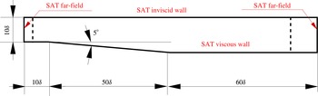
We apply the method to try to stabilize a separated boundary layer within a duct. Figure 1 shows the computational domain and the boundary conditions for the flow under consideration. The incoming flow is a Mach 0.65 (free stream) boundary layer at a Reynolds number of
 $c_{\infty }\unicode[STIX]{x1D6FF}/\unicode[STIX]{x1D708}=250$
. The grid size used for the present simulation is
 $(N_{\unicode[STIX]{x1D709}},N_{\unicode[STIX]{x1D702}})\equiv (1386,200)$
, in the streamwise and wall-normal directions, respectively.
Computational domain (drawn to scale,
 $\unicode[STIX]{x1D6FF}$
is the boundary layer thickness of the incoming boundary layer) showing the boundary conditions. The dotted lines denote the sponge zones.

3.3 Steady baseflow for the Mach 0.65 diffuser
The equilibrium baseflow solution for the Mach 0.65 diffuser was computed using the SFD method, with parameters
 $\unicode[STIX]{x1D712}=0.05$
and
 $\unicode[STIX]{x0394}=20.0$
(in the notation of Åkervik et al.
Reference Åkervik, Brandt, Henningson, Hœpffner, Marxen and Schlatter2006) estimated from the eigenanalysis of the unsteady flow field. Figure 2 shows the Mach number contours for the equilibrium baseflow
 $\boldsymbol{Q}_{e}$
for which the residual
 $||\tilde{\boldsymbol{R}}(\boldsymbol{Q}_{e})||_{\infty }$
was reduced to
 $10^{-11}$
over time
 $\unicode[STIX]{x0394}tc_{\infty }/\unicode[STIX]{x1D6FF}=10\,000$
. Mesh independence was established by verifying that the relevant portion of the global eigenspectrum for the steady baseflow showed very little change upon refinement (e.g. the change in the growth rate of the most unstable eigenmode was less than 0.02 % upon increasing the grid points by a factor of 2). Further quantitative comparisons of the growth rate of the global modes, those computed directly from the simulation, and those from the linear stability analysis, also showed that the simulation was well resolved (not shown).
Mach number contours at steady state.

3.4 Actuator–sensor selection
Controller selection and placement for localized linear feedback control requires the solution of the optimization problem (3.4), with
 $\tilde{\unicode[STIX]{x1D63E}}$
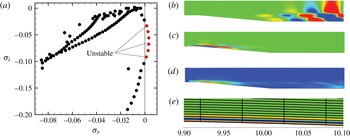
bounded, applied to a specific eigenvalue. To demonstrate the method we target the most unstable eigenvalue in figure 3(a), whose forward and adjoint global modes are shown in figure 3(b,c) and wavemaker
 $\unicode[STIX]{x1D706}$
in figure 3(d). Observe that the wavemaker shown in figure 3(d) suggests that the separated flow may be efficiently affected by a controller slightly downstream of the diffuser corner. However, it does not suggest which specific control/sensor pair(s) should be examined, nor does it yield a spatially precise location for actuation that is specific to the control/sensor pair.
To first demonstrate the methodology of controller selection and placement, we consider the constrained case of mass control with the forcing based on different feedback variables:
 $\unicode[STIX]{x1D70C}$
,
 $\unicode[STIX]{x1D70C}u$
,
 $\unicode[STIX]{x1D70C}v$
and
 $\unicode[STIX]{x1D70C}E$
. (The unconstrained case will be shown in §3.5.1.) The target eigenmode for optimization is the most unstable one (figure 3
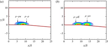
a). Figure 3(b–d) shows the eigenmodes and the wavemaker associated with the most unstable mode. As expected, the wavemaker indicates that the upstream corner of the diffuser is where the flow is most sensitive to active actuation. This result is consistent with that observed by Marquet et al. (Reference Marquet, Lombardi, Chomaz, Sipp and Jacquin2009). Figure 4 demonstrates the outcome of the present placement and optimization approach, showing the shape and location of the locally optimal actuation region for mass control for different control–feedback pairs. It is important to note that the shape, size, and location for optimal actuation is seen to depend on the type of control–feedback employed. The wavemaker
 $\unicode[STIX]{x1D706}$
does not provide this level of detail but gives, instead, a useful estimate on what may be expected. We did not observe any dependence on the initial conditions chosen for the optimization when using the Trust-Region-Reflective algorithm in MATLAB (Han Reference Han1977).
Discrete-adjoint eigenmodes have been shown to have oscillations close to the boundaries (Chandler et al. Reference Chandler, Juniper, Nichols and Schmid2012) when the underlying forward discretization is not dual consistent. Figure 3(e) shows that the near-wall oscillations are confined to just three grid points close to the boundary, and do not extend further into the domain. However, the discrete-adjoint approach gives the exact adjoint and facilitates identifying forward–adjoint pairs which correspond to the same eigenvalue. It is the overlap of this pair of forward and adjoint global modes that gives us the wavemaker, which is an essential part of the analysis. The continuous-adjoint approach avoids the unphysical oscillations, but the eigenvalue of the adjoint mode corresponding to a given forward mode can differ significantly (Chandler et al. Reference Chandler, Juniper, Nichols and Schmid2012), and hence the identification of a forward–adjoint pair becomes difficult.
(a) The eigenspectrum for the Mach 0.65 equilibrium baseflow in the diffuser; (b) forward eigenmode,
 $\text{Re}(\widehat{\unicode[STIX]{x1D70C}u})$
; (c) adjoint eigenmode,
 $\text{Re}(\widehat{\unicode[STIX]{x1D70C}u}^{\dagger })$
; (d) wavemaker as defined by (1.1); (e) near-wall zoom of the adjoint eigenmode.

Shape and location of the effective wavemaker for mass control for different control–feedback pairs: (a)
 $\unicode[STIX]{x1D70C}-\unicode[STIX]{x1D70C}$
and
 $\unicode[STIX]{x1D70C}-\unicode[STIX]{x1D70C}u$
, (b)
 $\unicode[STIX]{x1D70C}-\unicode[STIX]{x1D70C}v$
and
 $\unicode[STIX]{x1D70C}-\unicode[STIX]{x1D70C}E$
.

3.5 Control of vortex shedding in the Mach 0.65 diffuser
The actuator is now used to globally stabilize the system and control the vortex shedding in the diffuser.
The eigenspectrum shift as a function of the control gain
 $\unicode[STIX]{x1D6FC}$
:

 $\unicode[STIX]{x1D6FC}=0.0$
to
 $0.108$
. The controlled eigenvalue is indicated by ○ (red). The open symbols (▫) show the uncontrolled eigenspectrum.

3.5.1 Global stabilization using linear feedback control
To study the effect of the increased control gain on the system, consider
 $\unicode[STIX]{x1D70C}$
–
 $\unicode[STIX]{x1D70C}$
control–feedback, as specified via
 $\tilde{\unicode[STIX]{x1D63E}}$
in (3.2). The global eigenanalysis of the closed-loop system
 $\unicode[STIX]{x1D63C}+\unicode[STIX]{x1D6FC}\unicode[STIX]{x1D63E}$
was performed with different values of the gain
 $\unicode[STIX]{x1D6FC}$
to obtain the range of values for which the system was globally stabilized (figure 5). Although the control was developed targeting the most unstable eigenvalue, there is ‘parasitic’ movement of other eigenvalues as well. In general, such a parasitic movement of eigenvalues need not be favourable. Since the estimate for the eigenvalue shift,
 $\unicode[STIX]{x1D6FF}\unicode[STIX]{x1D70E}$
, given by (3.3) is linear in the coefficients
 $c_{ij}$
(a result that follows from assuming
 $\unicode[STIX]{x1D6FF}\unicode[STIX]{x1D63C}=\unicode[STIX]{x1D6FC}\unicode[STIX]{x1D63E}$
is suitably small so that products of perturbed quantities can be neglected), the actual eigenvalue shift as
 $\unicode[STIX]{x1D63C}$
is perturbed to
 $\unicode[STIX]{x1D63C}+\unicode[STIX]{x1D6FC}\unicode[STIX]{x1D63E}$
will begin to differ significantly from that obtained from the first-order structural sensitivity analysis of (3.3); namely that the spectrum of
 $\unicode[STIX]{x1D63C}+\unicode[STIX]{x1D6FC}\unicode[STIX]{x1D63E}$
is approximated by the spectrum of
 $\unicode[STIX]{x1D63C}$
plus a correction
 $\unicode[STIX]{x1D6FF}\unicode[STIX]{x1D70E}$
. It can be seen that for low values of control gain, the eigenspectrum tends to shift towards the left-hand plane (LHP), and for this flow achieves complete stabilization; for further increase in
 $\unicode[STIX]{x1D6FC}$
, some of the eigenvalues return to the right-hand plane (RHP). Global stability is achieved for
 $0.105<\unicode[STIX]{x1D6FC}_{stable}<0.108$
, whereas the linear estimate for the minimum control gain for stabilizing the most unstable eigenvalue was
 $\unicode[STIX]{x1D6FC}=0.32$
. As a consequence of this reversal of the eigenspectrum shift, there exists only a range of the control gain
 $\unicode[STIX]{x1D6FC}$
for which global stabilization can be achieved even in just the linear system.
It should be noted that there are numerous actuator–sensor combinations that include single as well as multiple control(s)–feedback(s) that could be developed using the algorithm. For the present flow, other feedback combinations using mass control were analysed as well. The root-locus diagram for the cases
 $\unicode[STIX]{x1D70C}-\unicode[STIX]{x1D70C}u$
,
 $\unicode[STIX]{x1D70C}-\unicode[STIX]{x1D70C}v$
and
 $\unicode[STIX]{x1D70C}-\unicode[STIX]{x1D70C}E$
are shown in figure 6(a–c), respectively. In the linear regime of structural sensitivity, the controller with maximum flexibility is the one that utilizes the full potential of the control matrix
 $\unicode[STIX]{x1D63E}$
. Such an actuator can be obtained by performing an unconstrained optimization by optimizing over all coefficients
 $c_{ij}$
of the control matrix
 $\unicode[STIX]{x1D63E}$
. For this case, we find that the estimated best actuator is, to within a constant,
 $$\begin{eqnarray}\displaystyle \tilde{\unicode[STIX]{x1D63E}}_{unconstrained}=\left[\begin{array}{@{}cccc@{}}1 & -1 & -1 & 1\\ -1 & 1 & 1 & -1\\ 1 & -1 & -1 & 1\\ -1 & 1 & -1 & -1\\ \end{array}\right]. & & \displaystyle\end{eqnarray}$$
The root-locus diagram for this controller is shown in figure 6(d). It can be seen that none of the above combinations could globally stabilize the system. The eigenspectrum shift, due to nonlinearity, pushes some of the eigenvalues back into the unstable regime. The ‘
 $\times$
’ (blue) mark in figure 6, and all subsequent root-locus diagrams, indicate the location in the eigenspace at which the error between the real parts of the predicted (from structural sensitivity) and the actual computed eigenvalues for a given control gain
 $\unicode[STIX]{x1D6FC}$
, reaches 1 %, i.e.
 $[(\unicode[STIX]{x1D70E}_{r})_{predicted}-(\unicode[STIX]{x1D70E}_{r})_{computed}]/(\unicode[STIX]{x1D70E}_{r})_{predicted}=0.01$
, where
 $(\unicode[STIX]{x1D70E}_{r})_{predicted}=(\unicode[STIX]{x1D70E}_{r})_{uncontrolled}+\unicode[STIX]{x1D6FF}\unicode[STIX]{x1D70E}_{structural~sensitivity}$
.
The eigenspectrum shift as a function of the control gain
 $\unicode[STIX]{x1D6FC}$
for mass control with different feedback combinations: (a)
 $\unicode[STIX]{x1D70C}-\unicode[STIX]{x1D70C}u$
, (b)
 $\unicode[STIX]{x1D70C}-\unicode[STIX]{x1D70C}v$
, (c)
 $\unicode[STIX]{x1D70C}-\unicode[STIX]{x1D70C}E$
, (d) unconstrained optimization.


3.5.2 Control of vortex shedding in the diffuser
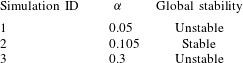
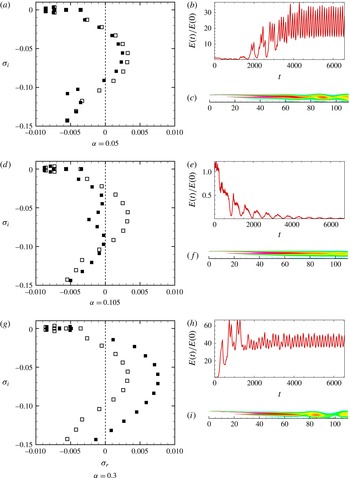
To confirm applicability to the actual, nonlinear flow, three different simulations were conducted with the same initial condition: the equilibrium baseflow perturbed with the most unstable eigenmode with the perturbation amplitude in the nonlinear regime (
 ${\sim}$
5 % of maximum amplitude). The actuation used
 $\unicode[STIX]{x1D70C}$
–
 $\unicode[STIX]{x1D70C}$
control–feedback. The control forcing term appears in the continuity equation as
 $$\begin{eqnarray}\displaystyle \frac{\unicode[STIX]{x2202}\unicode[STIX]{x1D70C}}{\unicode[STIX]{x2202}t}=\tilde{\boldsymbol{R}}_{\unicode[STIX]{x1D70C}}(\boldsymbol{Q})+\unicode[STIX]{x1D6FC}\text{e}^{-(x-x_{0})^{2}/\ell _{x}^{2}-(y-y_{0})^{2}/\ell _{y}^{2}}(\unicode[STIX]{x1D70C}-\unicode[STIX]{x1D70C}_{e}), & & \displaystyle\end{eqnarray}$$
where
 $\unicode[STIX]{x1D70C}_{e}$
is the steady baseflow density. The simulations performed and the observed system character corresponding to the actuator are given in table 1. We define the total perturbation kinetic energy in the system as
 $E(t)=\int _{{\mathcal{V}}}[u^{\prime }(t)^{2}+v^{\prime }(t)^{2}]\,\text{d}{\mathcal{V}}/2$
. The control objective,
 $E(t)/E(0)$
, is used to quantify the deviation of the system from the baseflow. Figure 7 shows the eigenspectrum and the unsteadiness quantification for the controlled flow for different values of the control gain. It can be seen that the control gain within the global stabilization window (
 $0.105<\unicode[STIX]{x1D6FC}<0.108$
) suppresses the vortex shedding downstream of the diffuser completely, whereas actuation with the gain value outside the stabilization window amplifies the initial perturbation energy of the system. The present Reynolds number was selected to illustrate this fundamental change of behaviour. It is noteworthy that other control–feedback methods can be developed with the present algorithm; however, identifying all such combinations was not part of the present work.
Direct numerical simulations to study the effect of control on vortex shedding.

(a,d,g) Eigenspectrum: ▫ uncontrolled, ▪ controlled. (b,e,h)
 $E(t)/E(0)$
for different control gains
 $\unicode[STIX]{x1D6FC}$
. (c,f,i) Contours of instantaneous vorticity. (a–c)
 $\unicode[STIX]{x1D6FC}=0.05$
; (d–f)
 $\unicode[STIX]{x1D6FC}=0.105$
; (g–i)
 $\unicode[STIX]{x1D6FC}=0.3$
.

3.6 More challenging-to-control configurations
The domain length and Reynolds number of the diffuser example were such that the control could completely suppress instabilities and stabilize the flow as simulated in the corresponding DNS. Of course, such efficacy is likely out of the question for higher Reynolds numbers and longer domains. Indeed, the information contained with the spectrum of
 $\unicode[STIX]{x1D63C}+\unicode[STIX]{x1D6FC}\unicode[STIX]{x1D63E}$
, as a function of
 $L_{x}$
and
 $Re$
, could be used to estimate the degree to which complete stabilization could be achieved. We choose to demonstrate the effect of these parameters by performing flow control for the following two additional cases for comparison. In the first case, the Reynolds number is held fixed at
 $Re=250$
, but the domain length is increased 50 % to
 $L_{x}=180\unicode[STIX]{x1D6FF}$
. In the second case, the domain length remains at
 $L_{x}=120\unicode[STIX]{x1D6FF}$
, but the Reynolds number is increased to 350. We further show that the ability to rationally select actuator/sensor pairs, and locate them, is robust to these changes.
3.6.1 Longer domain
To study the effect of the domain length, a steady baseflow was computed for the extended domain with
 $L_{x}/\unicode[STIX]{x1D6FF}=180$
at
 $Re=250$
and the results were compared to those from the original domain with
 $L_{x}/\unicode[STIX]{x1D6FF}=120$
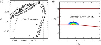
. Figure 8(a) shows that the unstable and least stable branch of the eigenspectrum is preserved for the short and long domains; but the long domain, on account of having a longer shear layer, supports more unstable modes (figure 9
a). The controllability analysis for
 $\unicode[STIX]{x1D63C}+\unicode[STIX]{x1D6FC}\unicode[STIX]{x1D63E}$
was performed for different values of the control gain
 $\unicode[STIX]{x1D6FC}$
for the long domain using the same control–feedback
 $\unicode[STIX]{x1D70C}-\unicode[STIX]{x1D70C}$
type with which global stabilization was observed for the short domain. Although the flow could not be globally stabilized for the longer domain, a significant reduction of the growth rate was observed for the unstable eigenvalues (
 ${\approx}$
50 % for the most unstable eigenvalue) (figure 9
b). It is well recognized that the global modes are sensitive to the domain size (Nichols & Lele Reference Nichols and Lele2011), so we anticipate the spectrum to have changed in this case, and streamwise decorrelation makes control over the full domain by localized actuation a fundamentally more challenging problem. Still the most unstable eigenvalue targeted by the control is suppressed and the overall flow rendered less amplifying by the informed control. We note that the actuator placement is essentially unchanged, as shown in figure 8(b). The longer domain analysis shows that the type of localized feedback control for a real, physical flow of this configuration may still depend on the type of outlet/length of the domain encountered by the flow downstream of separation.
(a) Eigenspectrum for the short and long domains at
 $Re=250$
:
 $L_{x}/\unicode[STIX]{x1D6FF}=120$
(▫);
 $L_{x}/\unicode[STIX]{x1D6FF}=180$
(
 $\times$
). (b) The controllers for the short and long domains almost overlap.

(a) Eigenspectrum for the short and long domains at
 $Re=250$
:
 $L_{x}/\unicode[STIX]{x1D6FF}=120$
(▫);
 $L_{x}/\unicode[STIX]{x1D6FF}=180$
(
 $\times$
). (b) Effect of the control gain (
 $\unicode[STIX]{x1D6FC}$
) on the eigenspectrum with
 $\unicode[STIX]{x1D70C}-\unicode[STIX]{x1D70C}$
control–feedback for the long domain at
 $Re=250$
: uncontrolled (
 $\times$
);
 $\unicode[STIX]{x1D6FC}=0.105$
(▿);
 $\unicode[STIX]{x1D6FC}=0.11$
(♢);
 $\unicode[STIX]{x1D6FC}=0.12$
(○).

3.6.2 Higher Reynolds number
A steady baseflow was computed at
 $Re=350$
for the short domain and the results were compared with the case at
 $Re=250$
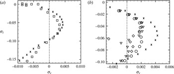
. Figure 10(a) shows the comparison of the eigenspectrum for the two baseflows. The effect of increasing the Reynolds number is qualitatively similar to that of the long domain at
 $Re=250$
, with more unstable eigenvalues and higher growth rates. Figure 10(b) shows the effect of increasing the control gain
 $\unicode[STIX]{x1D6FC}$
for the
 $\unicode[STIX]{x1D70C}$
–
 $\unicode[STIX]{x1D70C}$
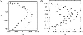
control–feedback, where it can be seen that the flow cannot be globally stabilized, but a significant reduction in the growth rate is obtained for all the unstable eigenvalues. The control was also performed using the actuator developed by unconstrained optimization as described in §3.5.1. The root-locus diagram (figure 11) shows that the reversal of the eigenspectrum shift occurs within a short range of the control gain (
 $0\leqslant \unicode[STIX]{x1D6FC}\leqslant 0.02$
), and hence global stabilization could not be achieved in this case as well.
The conclusion is that the complete suppression of instabilities is likely out of the question for higher Reynolds numbers and longer domains. Still, the present technique provided informed actuation that suppresses the instabilities even in these cases, though the flow is not, of course, fully stabilized.
Eigenspectrum for the short domain at two different Reynolds numbers:
 $Re=250$
(▫);
 $Re=350$
(○). (b) Effect of the control gain (
 $\unicode[STIX]{x1D6FC}$
) on the eigenspectrum with
 $\unicode[STIX]{x1D70C}-\unicode[STIX]{x1D70C}$
control–feedback for the short domain at
 $Re=350$
: uncontrolled (○);
 $\unicode[STIX]{x1D6FC}=0.05$
(
 $\times$
);
 $\unicode[STIX]{x1D6FC}=0.10$
(♢);
 $\unicode[STIX]{x1D6FC}=0.20$
(▵).

Effect of the control gain (
 $\unicode[STIX]{x1D6FC}$
) on the eigenspectrum for the unconstrained actuator for the baseflow at
 $Re=350$
(
 $0\leqslant \unicode[STIX]{x1D6FC}\leqslant 0.02$
).


4 Conclusions
This paper develops an extended structural sensitivity analysis that can be used to estimate profitable types and locations of actuators and sensors in a flow control scenario. Using the information contained in the forward and adjoint global modes of the uncontrolled baseflow, an optimization problem is presented that scales linearly in the number of actuators and sensors, but is independent of the dimensionality of the underlying discretized problem. The method is applied to the stabilization of a separated boundary layer within an asymmetric diffuser at Mach 0.65, where the spectrum of the linearized, closed-loop system describes well the behaviour of the fully nonlinear system. Potential generalizations of the method are also discussed.
Acknowledgements
Financial support from Rolls-Royce North America (Dr J. Sokhey, technical monitor) and the Office of Naval Research (Drs J. Doychak, K. Millsaps and B. Henderson, technical monitors) is gratefully acknowledged. This material is also based in part upon work supported by the Department of Energy, National Nuclear Security Administration, under Award Number DE-NA0002374. Financial support from the Center for Turbulence Research Summer Program for D.J.B. is also gratefully acknowledged.