Natural convection in a corrugated slot

Arman Abtahi; J. M. Floryan

doi:10.1017/jfm.2017.73

Natural convection in a corrugated slot

Published online by Cambridge University Press: 23 February 2017

Arman Abtahi

and

J. M. Floryan

Show author details

Arman Abtahi*: Affiliation:
Department of Mechanical and Materials Engineering, University of Western Ontario, London, Ontario, N6A 5B9, Canada
J. M. Floryan: Affiliation:
Department of Mechanical and Materials Engineering, University of Western Ontario, London, Ontario, N6A 5B9, Canada
*: †Email address for correspondence: sabtahi4@uwo.ca

Article contents

Abstract
Introduction
Problem formulation
Corrugation at the lower plate
Corrugation at the upper plate
Corrugations at both plates
Effects of Prandtl number
Conclusions
References

Rights & Permissions

Abstract

Analysis of natural convection in a horizontal slot formed by two corrugated isothermal plates has been carried out. The analysis is limited to subcritical Rayleigh numbers $Ra$ where no secondary motion takes place in the absence of corrugations. The corrugations have a sinusoidal form characterized by the wavenumber, the upper and lower amplitudes and the phase difference. The most intense convection occurs for corrugation wavelengths comparable to the slot height; it increases proportionally to $Ra$ and proportionally to the corrugation height. Placement of corrugations on both plates may either significantly increase or decrease the convection depending on the phase difference between the upper and lower corrugations, with the strongest convection found for corrugations being in phase, i.e. a ‘wavy’ slot, and the weakest for corrugations being out of phase, i.e. a ‘converging–diverging’ slot. It is shown that the shear forces would always contribute to the corrugation build-up if erosion was allowed, while the role of pressure forces depends on the location of the corrugations as well as on the corrugation height and wavenumber, and the Rayleigh number. Placing corrugations on both plates results in the formation of a moment which attempts to change the relative position of the plates. There are two limiting positions, i.e. the ‘wavy’ slot and the ‘converging–diverging’ slot, with the latter being unstable. The system would end up in the ‘wavy’ slot configuration if relative movement of the two plates was allowed. The presence of corrugations affects the conductive heat flow and creates a convective heat flow. The conductive heat flow increases with the corrugation height as well as with the corrugation wavenumber; it is largest for short-wavelength corrugations. The convective heat flow is relevant only for wavenumbers of $O(1)$ , it increases proportionally to $Ra^{3}$ and proportionally to the second power of the corrugation height. Convection is qualitatively similar for all Prandtl numbers $Pr$ , with its intensity increasing for smaller $Pr$ and with the heat transfer augmentation increasing for larger $Pr$ .

JFM classification

Convection: Convection

Information

Type: Papers
Information: Journal of Fluid Mechanics , Volume 815 , 25 March 2017, pp. 537 - 569
DOI: https://doi.org/10.1017/jfm.2017.73 [Opens in a new window]
Copyright: © 2017 Cambridge University Press

1 Introduction

Natural convection in a horizontal slot is typically associated with spatially homogeneous heating applied at the lower surface and is referred to as Rayleigh–Bénard (RB) convection (Bénard Reference Bénard1900; Rayleigh Reference Rayleigh1916). It results from transition from a conductive state when the critical conditions are exceeded (Bodenschatz, Pesch & Ahlers Reference Bodenschatz, Pesch and Ahlers2000; Ahlers, Grossmann & Lohse Reference Ahlers, Grossmann and Lohse2009; Lohse & Xia Reference Lohse and Xia2010; Chilla & Schumacher Reference Chilla and Schumacher2012), and it changes the character of the heat flow in qualitative terms. The onset can be affected by inhomogeneities in the boundary temperatures (Freund, Pesch & Zimmermann Reference Freund, Pesch and Zimmermann2011) as well as by inhomogeneities in the surface geometry (McCoy et al. Reference McCoy, Brunner, Pesch and Bodenschatz2008; Seiden et al. Reference Seiden, Weiss, McCoy, Pesch and Bodenschatz2008; Weiss, Seiden & Bodenschatz Reference Weiss, Seiden and Bodenschatz2012) resulting in various forms of symmetry breaking.

Inhomogeneous heating creates horizontal density variations which lead to horizontal and vertical temperature gradients resulting in motions frequently referred to as horizontal convection (Maxworthy Reference Maxworthy1997; Siggers, Kerswell & Balmforth Reference Siggers, Kerswell and Balmforth2004; Hughes & Griffiths Reference Hughes and Griffiths2008; Winters & Young Reference Winters and Young2009). Identical motions can be generated by the same heating applied either from below or from above if one accounts for the up/down symmetry (Hossain & Floryan Reference Hossain and Floryan2014). The flow topology is locked in with the heating pattern but only for small convection intensity. Higher intensities result in transition to secondary states which might have different patterns (Hossain & Floryan Reference Hossain and Floryan2013b ). As there are an uncountable number of heating patterns, recent studies have been focused on the simplest pattern, consisting of sinusoidal heating with an arbitrary wavelength (Hossain & Floryan Reference Hossain and Floryan2013a ), and have led to the concept of structured convection. There are numerous examples of such convection, e.g. circulation in urban environments as local heating rates are determined by the dissimilar thermal properties of roofs, streets and parks, and circulation in rural environments where local circulation is driven by variations in the heating rates of forests, fields and lakes. Convection within the Earth’s mantle is affected by the insulating effect of continents and represents a spatially structured convection with heating from above (Lenardic et al. Reference Lenardic, Moresi, Jellinek and Manga2005). A system of fractures, leads and polynyas in sea ice leads to convection in both the ocean and the atmosphere (Marcq & Weiss Reference Marcq and Weiss2012). Use of mixed insulating and conducting boundary conditions leads to a spatially patterned convection (Ripesi et al. Reference Ripesi, Biferale, Sbragaglia and Wirth2014). Human activity resulting in the heat island effect (Rizwam, Dennis & Liu Reference Rizwam, Dennis and Liu2008) can be analysed from the heating pattern point of view. The dynamics of a system of localized fires and prediction of their propagation represent another challenging problem (Finney et al. Reference Finney, Cohen, McAllister and Jolly2012) similar to thermal patterning in microfluidic devices (Krishnan, Ugaz & Burns Reference Krishnan, Ugaz and Burns2002; Beltrame et al. Reference Beltrame, Knobloch, Hänggi and Thiele2011).

This analysis is focused on natural convection in a slot formed by two horizontal corrugated plates and is aimed at understanding the natural convection in the presence of geometric non-uniformities. Because of an uncountable number of forms of such non-uniformities, we have selected a simple reference case involving sinusoidal corrugations whose geometry is characterized in terms of the corrugation wavenumber and the corrugation amplitude. Placement of corrugations on both walls adds a second amplitude as well as a phase difference describing the relative position of the two corrugation systems to the set of geometric parameters. In all cases, the plates are kept isothermal and, thus, the heating intensity is always expressed in terms of the same Rayleigh number. Such systems occur frequently in nature, e.g. hills and valleys in rural environments and geometric patterning of microfluidic devices (Krishnan et al. Reference Krishnan, Ugaz and Burns2002; Beltrame et al. Reference Beltrame, Knobloch, Hänggi and Thiele2011), among many others. The problem of convection between biological membranes is especially interesting due their potential deformation driven by convection-generated forces. Our interest is in the subcritical heating conditions where the system represents a conductive state of equilibrium in the limit of smooth plates. Addition of corrugations results in a conductive state that has both horizontal and vertical temperature gradients. It can be shown that this is not a state of equilibrium for fluids and, thus, a motion must occur regardless of the intensity of the heating. Section 2 provides the formulation of the model problem. Section 3 discusses convection when only the lower plate is corrugated; § 3.1 discusses convection associated with long-wavelength corrugations while § 3.2 deals with convection associated with corrugations of arbitrary wavelengths. Section 4 describes convection resulting from corrugating the upper plate. Section 5 is devoted to the description of convection when both plates are corrugated; § 5.1 discusses the role of long-wavelength corrugations while § 5.2 describes convection associated with corrugations of arbitrary wavelengths. All results presented in §§ 3–5 have been determined for a Prandtl number of $Pr=0.71$ . Section 6 extends the analysis to arbitrary Prandtl numbers. Section 7 provides a short summary of the main conclusions.

2 Problem formulation

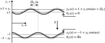
Consider fluid contained in a slot formed by two horizontal corrugated plates (see figure 1) with geometries specified as

(2.1a )

$$\begin{eqnarray}\displaystyle & \displaystyle y_{L}^{\ast }(x^{\ast })=-h^{\ast }+C_{L}^{\ast }\cos (\unicode[STIX]{x1D6FC}^{\ast }x^{\ast }), & \displaystyle\end{eqnarray}$$

(2.1b )

$$\begin{eqnarray}\displaystyle & \displaystyle y_{U}^{\ast }(x^{\ast })=h^{\ast }+C_{U}^{\ast }\cos (\unicode[STIX]{x1D6FC}^{\ast }x^{\ast }+\unicode[STIX]{x1D6FA}_{C}^{\ast }), & \displaystyle\end{eqnarray}$$

where the subscripts

$L$ and

$U$ refer to the lower and upper plate respectively,

$C_{L}^{\ast }$ and

$C_{U}^{\ast }$ are the corrugation amplitudes at the lower and upper plates respectively,

$\unicode[STIX]{x1D6FA}_{C}^{\ast }$ stands for the phase shift between the two corrugation systems,

$\unicode[STIX]{x1D6FC}^{\ast }$ is the corrugation wavenumber and stars denote dimensional quantities. The slot extends to

$\pm \infty$ in the

$x$ -direction and is periodic with wavelength

$\unicode[STIX]{x1D706}^{\ast }=2\unicode[STIX]{x03C0}/\unicode[STIX]{x1D6FC}^{\ast }$ , with the mean distance between the plates being

$2h^{\ast }$ . Gravitational acceleration

$g^{\ast }$ is acting in the negative

$y$ -direction. The lower and upper plates are kept isothermal at temperatures

$T_{L}^{\ast }$ and

$T_{U}^{\ast }$ respectively. We select

$T_{U}^{\ast }$ as the reference temperature for evaluation of all material properties. The fluid has thermal conductivity

$k^{\ast }$ , specific heat

$c^{\ast }$ , thermal diffusivity

$\unicode[STIX]{x1D705}^{\ast }=k^{\ast }/\unicode[STIX]{x1D70C}^{\ast }c^{\ast }$ , kinematic viscosity

$\unicode[STIX]{x1D708}^{\ast }$ , dynamic viscosity

$\unicode[STIX]{x1D707}^{\ast }$ , thermal expansion coefficient

$\unicode[STIX]{x1D6E4}^{\ast }$ , and variations of the density

$\unicode[STIX]{x1D70C}^{\ast }$ follow the Boussinesq approximation.

Figure 1.

Schematic diagram of the flow system.

We define the relative temperature as $\unicode[STIX]{x1D703}^{\ast }=T^{\ast }-T_{U}^{\ast }$ , which leads to thermal boundary conditions of the form

(2.2a,b )

$$\begin{eqnarray}\displaystyle \unicode[STIX]{x1D703}_{L}^{\ast }(y_{L}^{\ast })=\unicode[STIX]{x1D703}_{S}^{\ast },\quad \unicode[STIX]{x1D703}_{U}^{\ast }(y_{U}^{\ast })=0, & & \displaystyle\end{eqnarray}$$

where $\unicode[STIX]{x1D703}_{S}^{\ast }=T_{L}^{\ast }-T_{U}^{\ast }$ . Use of the half of the mean distance between the plates $h^{\ast }$ as the length scale and $\unicode[STIX]{x1D705}^{\ast }\unicode[STIX]{x1D708}^{\ast }/(g^{\ast }\unicode[STIX]{x1D6E4}^{\ast }h^{\ast 3})$ as the temperature scale results in the following expressions for the geometry and temperatures:

(2.3a,b )

$$\begin{eqnarray}\displaystyle y_{L}(x)=-1+y_{b}\cos (\unicode[STIX]{x1D6FC}x),\quad y_{U}(x)=1+y_{t}\cos (\unicode[STIX]{x1D6FC}x+\unicode[STIX]{x1D6FA}_{C}), & & \displaystyle\end{eqnarray}$$

(2.4a,b )

$$\begin{eqnarray}\displaystyle \unicode[STIX]{x1D703}_{L}(y_{L})=Ra,\quad \unicode[STIX]{x1D703}_{U}(y_{U})=0, & & \displaystyle\end{eqnarray}$$

where $y_{b}>0$ and $y_{t}>0$ are the amplitudes of the corrugations on the lower and upper plates respectively and $Ra=g^{\ast }\unicode[STIX]{x1D6E4}^{\ast }h^{\ast 3}\unicode[STIX]{x1D703}_{S}^{\ast }/(\unicode[STIX]{x1D705}^{\ast }\unicode[STIX]{x1D708}^{\ast })$ is the Rayleigh number measuring the intensity of the heating. The field equations have the following form:

(2.5a,b )

$$\begin{eqnarray}\displaystyle \frac{\unicode[STIX]{x2202}u}{\unicode[STIX]{x2202}x}+\frac{\unicode[STIX]{x2202}v}{\unicode[STIX]{x2202}y}=0,\quad u\frac{\unicode[STIX]{x2202}u}{\unicode[STIX]{x2202}x}+v\frac{\unicode[STIX]{x2202}u}{\unicode[STIX]{x2202}y}=-\frac{\unicode[STIX]{x2202}p}{\unicode[STIX]{x2202}x}+\unicode[STIX]{x1D6FB}^{2}u, & & \displaystyle\end{eqnarray}$$

(2.5c,d )

$$\begin{eqnarray}\displaystyle u\frac{\unicode[STIX]{x2202}v}{\unicode[STIX]{x2202}x}+v\frac{\unicode[STIX]{x2202}v}{\unicode[STIX]{x2202}y}=-\frac{\unicode[STIX]{x2202}p}{\unicode[STIX]{x2202}y}+\unicode[STIX]{x1D6FB}^{2}v+Pr^{-1}\unicode[STIX]{x1D703},\quad u\frac{\unicode[STIX]{x2202}\unicode[STIX]{x1D703}}{\unicode[STIX]{x2202}x}+v\frac{\unicode[STIX]{x2202}\unicode[STIX]{x1D703}}{\unicode[STIX]{x2202}y}=Pr^{-1}\unicode[STIX]{x1D6FB}^{2}\unicode[STIX]{x1D703}, & & \displaystyle\end{eqnarray}$$

where ( $u$ , $v$ ) are the velocity components in the ( $x$ , $y$ )-directions respectively, scaled with $U_{v}^{\ast }=\unicode[STIX]{x1D708}^{\ast }/h^{\ast }$ , $p$ stands for the pressure scaled with $\unicode[STIX]{x1D70C}^{\ast }U_{\unicode[STIX]{x1D708}}^{\ast 2}$ and $Pr=\unicode[STIX]{x1D708}^{\ast }/\unicode[STIX]{x1D705}^{\ast }$ is the Prandtl number. These equations are subject to velocity boundary conditions of the form

(2.6a,b )

$$\begin{eqnarray}\displaystyle u(y_{L})=u(y_{U})=0,\quad v(y_{L})=v(y_{U})=0 & & \displaystyle\end{eqnarray}$$

as well as the thermal boundary conditions (2.4). There is no externally imposed horizontal pressure gradient, and this condition can be expressed as

(2.6c )

$$\begin{eqnarray}\displaystyle \left.\frac{\unicode[STIX]{x2202}p}{\unicode[STIX]{x2202}x}\right|_{mean}=0. & & \displaystyle\end{eqnarray}$$

The system (2.5)–(2.6) is solved by expressing the unknowns as Fourier expansions of the form

(2.7a )

$$\begin{eqnarray}\displaystyle & \displaystyle [u(x,y),v(x,y)]=\mathop{\sum }_{n=-\infty ,n\neq 0}^{n=+\infty }[u^{(n)}(y),v^{(n)}(y)]\text{e}^{\text{i}n\unicode[STIX]{x1D6FC}x}, & \displaystyle\end{eqnarray}$$

(2.7b )

$$\begin{eqnarray}\displaystyle & \displaystyle [\unicode[STIX]{x1D703}(x,y),p(x,y)]=\mathop{\sum }_{n=-\infty }^{n=+\infty }[\unicode[STIX]{x1D703}^{(n)}(y),p^{(n)}(y)]\text{e}^{\text{i}n\unicode[STIX]{x1D6FC}x}, & \displaystyle\end{eqnarray}$$

where

$u^{(n)}(y),v^{(n)}(y),p^{(n)}(y),\unicode[STIX]{x1D703}^{(n)}(y)$ denote the modal functions which are expressed in terms of the Chebyshev expansions. The Galerkin procedure is used to construct the algebraic system for the expansion coefficients, and the immersed boundary conditions method (IBC) is used to account for the irregularity of the solution domain. Condition (2.6c ) is satisfied automatically due to the form of (2.7). The pressure field is normalized in such a way that

$p(0,0)=C$ , where

$C$ is an arbitrary constant. Details of this spectrally accurate algorithm can be found in (Husain & Floryan 2010; Abtahi, Hossain & Floryan 2016).

Analysis of the system dynamics requires evaluation of the forces acting on the plates. The stress vector $\unicode[STIX]{x1D748}_{L}$ acting on the lower plate can be expressed as

(2.8)

$$\begin{eqnarray}\displaystyle \unicode[STIX]{x1D748}_{L}=\left[\begin{array}{@{}c@{}}\unicode[STIX]{x1D70E}_{x,L},\unicode[STIX]{x1D70E}_{y,L}\end{array}\right]=\left[\begin{array}{@{}c@{}}n_{x,L},n_{y,L}\end{array}\right]\left[\begin{array}{@{}cc@{}}\unicode[STIX]{x1D70F}_{xx}+p & \unicode[STIX]{x1D70F}_{xy}\\ \unicode[STIX]{x1D70F}_{yx} & \unicode[STIX]{x1D70F}_{yy}+p\end{array}\right]_{y_{L}}, & & \displaystyle\end{eqnarray}$$

where

(2.9a-c )

$$\begin{eqnarray}\displaystyle \unicode[STIX]{x1D70F}_{xx}=-2\frac{\unicode[STIX]{x2202}u}{\unicode[STIX]{x2202}x},\quad \unicode[STIX]{x1D70F}_{xy}=\unicode[STIX]{x1D70F}_{yx}=-\frac{\unicode[STIX]{x2202}u}{\unicode[STIX]{x2202}y}-\frac{\unicode[STIX]{x2202}v}{\unicode[STIX]{x2202}x},\quad \unicode[STIX]{x1D70F}_{yy}=-2\frac{\unicode[STIX]{x2202}v}{\unicode[STIX]{x2202}y} & & \displaystyle\end{eqnarray}$$

are the components of the shear tensor and

(2.10)

$$\begin{eqnarray}\displaystyle [n_{x,L},n_{y,L}]=N_{L}[-\unicode[STIX]{x1D6FC}y_{b}\sin (\unicode[STIX]{x1D6FC}x),-1] & & \displaystyle\end{eqnarray}$$

stands for the normal unit vector pointing outwards, with $N_{L}=\{1+[\unicode[STIX]{x1D6FC}y_{b}\sin (\unicode[STIX]{x1D6FC}x)]^{2}\}^{-1/2}$ . The $x$ and $y$ components of the stress vector have the following forms:

(2.11a )

$$\begin{eqnarray}\displaystyle \unicode[STIX]{x1D70E}_{x,L} & = & \displaystyle \unicode[STIX]{x1D70E}_{xv,L}+\unicode[STIX]{x1D70E}_{xp,L}=N_{L}\!\left[2\unicode[STIX]{x1D6FC}y_{b}\sin (\unicode[STIX]{x1D6FC}x)\left.\frac{\unicode[STIX]{x2202}u}{\unicode[STIX]{x2202}x}\right|_{y_{L}}+\!\left.\left(\frac{\unicode[STIX]{x2202}u}{\unicode[STIX]{x2202}y}+\frac{\unicode[STIX]{x2202}v}{\unicode[STIX]{x2202}x}\right)\right|_{y_{L}}\right]-N_{L}\unicode[STIX]{x1D6FC}y_{b}\sin (\unicode[STIX]{x1D6FC}x)\left.p\right|_{y_{L}},\nonumber\\ \displaystyle & & \displaystyle\end{eqnarray}$$

(2.11b )

$$\begin{eqnarray}\displaystyle \unicode[STIX]{x1D70E}_{y,L} & = & \displaystyle \unicode[STIX]{x1D70E}_{yv,L}+\unicode[STIX]{x1D70E}_{yp,L}=N_{L}\!\left[\unicode[STIX]{x1D6FC}y_{b}\sin (\unicode[STIX]{x1D6FC}x)\left.\left(\frac{\unicode[STIX]{x2202}u}{\unicode[STIX]{x2202}y}+\!\frac{\unicode[STIX]{x2202}v}{\unicode[STIX]{x2202}x}\right)\right|_{y_{L}}+2\left.\frac{\unicode[STIX]{x2202}v}{\unicode[STIX]{x2202}y}\right|_{y_{L}}\right]-N_{L}\left.p\right|_{y_{L}},\end{eqnarray}$$

where $(\unicode[STIX]{x1D70E}_{xv,L},\unicode[STIX]{x1D70E}_{yv,L})$ and $(\unicode[STIX]{x1D70E}_{xp,L},\unicode[STIX]{x1D70E}_{yp,L})$ denote the viscous and pressure contributions respectively. The normal $\unicode[STIX]{x1D70E}_{n,L}$ and tangential $\unicode[STIX]{x1D70E}_{t,L}$ components can be expressed as

(2.11c )

$$\begin{eqnarray}\displaystyle \unicode[STIX]{x1D70E}_{n,L} & = & \displaystyle \unicode[STIX]{x1D70E}_{nv,L}+\unicode[STIX]{x1D70E}_{np,L}=N_{L}^{2}\left[-2\unicode[STIX]{x1D6FC}^{2}y_{b}^{2}\sin ^{2}(\unicode[STIX]{x1D6FC}x)\left.\frac{\unicode[STIX]{x2202}u}{\unicode[STIX]{x2202}x}\right|_{y_{L}}\right.\nonumber\\ \displaystyle & & \displaystyle \left.-\,2\unicode[STIX]{x1D6FC}y_{b}\sin (\unicode[STIX]{x1D6FC}x)\left.\left(\frac{\unicode[STIX]{x2202}u}{\unicode[STIX]{x2202}y}+\frac{\unicode[STIX]{x2202}v}{\unicode[STIX]{x2202}x}\right)\right|_{y_{L}}-2\left.\frac{\unicode[STIX]{x2202}v}{\unicode[STIX]{x2202}y}\right|_{y_{L}}\right]+\left.p\right|_{y_{L}},\end{eqnarray}$$

(2.11d )

$$\begin{eqnarray}\displaystyle \unicode[STIX]{x1D70E}_{t,L} & = & \displaystyle N_{L}^{2}\left\{2\unicode[STIX]{x1D6FC}y_{b}\sin (\unicode[STIX]{x1D6FC}x)\left.\left(\frac{\unicode[STIX]{x2202}u}{\unicode[STIX]{x2202}x}-\frac{\unicode[STIX]{x2202}v}{\unicode[STIX]{x2202}y}\right)\right|_{y_{L}}+\left[1-\unicode[STIX]{x1D6FC}^{2}y_{b}^{2}\sin ^{2}(\unicode[STIX]{x1D6FC}x)\right]\left.\left(\frac{\unicode[STIX]{x2202}u}{\unicode[STIX]{x2202}y}+\frac{\unicode[STIX]{x2202}v}{\unicode[STIX]{x2202}x}\right)\right|_{y_{L}}\right\},\nonumber\\ \displaystyle & & \displaystyle\end{eqnarray}$$

where $\unicode[STIX]{x1D70E}_{nv,L}$ and $\unicode[STIX]{x1D70E}_{np,L}$ denote the viscous and pressure contributions to the normal component respectively. The heat transfer characteristics are expressed in terms of the local Nusselt number $Nu_{loc,L}$ , defined as

(2.12)

$$\begin{eqnarray}\displaystyle Nu_{loc,L}=\boldsymbol{n}_{L}\boldsymbol{\cdot }\boldsymbol{q}_{L}=n_{x,L}q_{x,L}+n_{y,L}q_{y,L}, & & \displaystyle\end{eqnarray}$$

where $\boldsymbol{q}_{L}=[q_{x,L},q_{y,L}]=[(\unicode[STIX]{x2202}\unicode[STIX]{x1D703}/\unicode[STIX]{x2202}x),(\unicode[STIX]{x2202}\unicode[STIX]{x1D703}/\unicode[STIX]{x2202}y)]_{y_{L}}$ stands for the temperature gradient at the wall. The net heat flux leaving the plate is expressed in terms of the mean Nusselt number $Nu_{av,L}$ defined as

(2.13)

$$\begin{eqnarray}\displaystyle Nu_{av}=\unicode[STIX]{x1D706}^{-1}\int _{0}^{\unicode[STIX]{x1D706}}Nu_{loc,L}N_{L}^{-1}\,\text{d}x. & & \displaystyle\end{eqnarray}$$

Similar relations can be developed for the upper plate, and the relevant quantities are identified using subscript $U$ . The reader may note that $N_{U}=\{1+[\unicode[STIX]{x1D6FC}y_{t}\sin (\unicode[STIX]{x1D6FC}x+\unicode[STIX]{x1D6FA}_{C})]^{2}\}^{-1/2}$ in this case.

The reader may note that convection does not occur in the absence of heating, i.e. $(u,v,\unicode[STIX]{x1D703})\rightarrow 0$ , $p\rightarrow C$ , $\unicode[STIX]{x1D70E}_{xv,L}\rightarrow 0,\unicode[STIX]{x1D70E}_{xp,L}\rightarrow -N_{L}\unicode[STIX]{x1D6FC}y_{b}\sin (\unicode[STIX]{x1D6FC}x)C$ , $\unicode[STIX]{x1D70E}_{yv,L}\rightarrow 0,\unicode[STIX]{x1D70E}_{yp,L}\rightarrow -N_{L}C$ when $Ra\rightarrow 0$ . Similarly, convection does not occur in a smooth heated slot for the subcritical $Ra$ values considered in this study, i.e. $(u,v)\rightarrow 0$ , $\unicode[STIX]{x1D703}\rightarrow (Ra/2)(1-y)$ , $p\rightarrow (Ra/2Pr)(-(y^{2}/2)+y)+C$ , $\unicode[STIX]{x1D70E}_{xv,L}\rightarrow 0$ , $\unicode[STIX]{x1D70E}_{xp,L}\rightarrow 0$ , $\unicode[STIX]{x1D70E}_{yv,L}\rightarrow 0,\unicode[STIX]{x1D70E}_{yp,L}\rightarrow -(3Ra/4Pr)+C$ when $(y_{b},y_{t})\rightarrow 0$ .

It is convenient for interpretation purposes to define a corresponding conduction problem, i.e.

(2.14a-c )

$$\begin{eqnarray}\displaystyle \unicode[STIX]{x1D6FB}^{2}\unicode[STIX]{x1D703}_{cond}=0,\quad \unicode[STIX]{x1D703}_{cond,L}(y_{L})=Ra,\quad \unicode[STIX]{x1D703}_{cond,U}(y_{U})=0, & & \displaystyle\end{eqnarray}$$

which can be solved using an algorithm adapted from Husain & Floryan (Reference Husain and Floryan2007). One can also define the conductive Nusselt numbers of the form

(2.15)

$$\begin{eqnarray}\displaystyle \left.\begin{array}{@{}c@{}}\displaystyle Nu_{cond,loc,L}=\boldsymbol{n}_{L}\boldsymbol{\cdot }\boldsymbol{q}_{c,L}=n_{x,L}\left.\frac{\unicode[STIX]{x2202}\unicode[STIX]{x1D703}_{c}}{\unicode[STIX]{x2202}x}\right|_{L}+n_{y,L}\left.\frac{\unicode[STIX]{x2202}\unicode[STIX]{x1D703}_{c}}{\unicode[STIX]{x2202}y}\right|_{L},\\ \displaystyle Nu_{cond,av}=\unicode[STIX]{x1D706}^{-1}\int _{0}^{\unicode[STIX]{x1D706}}Nu_{cond,loc,L}N_{L}^{-1}\,\text{d}x.\end{array}\right\} & & \displaystyle\end{eqnarray}$$

3 Corrugation at the lower plate

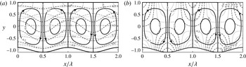
A typical pattern of motion resulting from the heating is illustrated in figure 2. The conductive temperature field in the absence of corrugations is uniform in the $x$ -direction and the fluid movement may occur only if the vertical temperature gradient meets critical conditions (Chandrasekhar Reference Chandrasekhar1961). The presence of corrugations generates horizontal conductive temperature gradients which lead to the formation of horizontal and vertical pressure gradients which drive the motion. The fluid moves upwards above the corrugation peaks and downwards above the corrugation troughs, resulting in the formation of counter-rotating horizontal rolls. The topologies of the pressure fields at the top and bottom of the slot are different due to the presence of a static component, as documented by plots of the pressure field with the mode zero $p^{(0)}(y)$ removed displayed in figure 2(b). The motion occurs regardless of the intensity of the heating and its characteristics are dictated by the corrugation geometry. We shall now focus on the detailed description of this motion, starting with long-wavelength corrugations.

Figure 2.

The flow, temperature and pressure fields for $\unicode[STIX]{x1D6FC}=1.53,Ra=200$ , $y_{b}=0.1$ , $C=0$ normalized with their maxima (a). The solid, dashed, dashed–dotted and dotted lines identify streamlines, isotherms of the complete temperature field, lines of constant pressure and isotherms of the conductive temperature field respectively. The maxima are $|\unicode[STIX]{x1D713}|_{max}=1.145,|\unicode[STIX]{x1D703}|_{max}=200$ , $|p|_{max}=213.7$ and $|\unicode[STIX]{x1D703}_{cond}|_{max}=200$ . The pressure field without mode zero is displayed in (b), with dashed and dotted lines identifying its positive and negative values, while dashed–dotted lines mark the zero isolines; $|p|_{max}=24.67$ .

3.1 Long-wavelength corrugation

Determination of the solution in the limit of $\unicode[STIX]{x1D6FC}\rightarrow 0$ begins with a domain transformation of the form

(3.1a,b )

$$\begin{eqnarray}\displaystyle \unicode[STIX]{x1D709}=\unicode[STIX]{x1D6FC}x,\quad \unicode[STIX]{x1D702}=2\frac{y-1}{2-y_{b}\cos \unicode[STIX]{x1D709}}+1, & & \displaystyle\end{eqnarray}$$

where $\unicode[STIX]{x1D709}$ is a slow scale and $\unicode[STIX]{x1D702}$ maps the corrugated slot onto a regular strip $\unicode[STIX]{x1D702}\in$ $[-1,1]$ . The unknowns are represented as power expansions in terms of $\unicode[STIX]{x1D6FC}$ , these expansions are substituted into the field equations, the leading-order systems are extracted and solved, with details given in appendix A. Solution of the conduction problem (2.14) has been obtained in a similar manner (details not given). The approximate solutions are used to determine wall stresses as well as heat fluxes. The stresses have the following forms:

(3.2a )

$$\begin{eqnarray}\displaystyle \unicode[STIX]{x1D70E}_{xv,L} & = & \displaystyle \unicode[STIX]{x1D70E}_{t,L}=-\unicode[STIX]{x1D6FC}\frac{y_{b}Ra}{Pr}\left[\frac{1}{10}\sin \unicode[STIX]{x1D709}-\frac{y_{b}}{40}\sin (2\unicode[STIX]{x1D709})\right]+O(\unicode[STIX]{x1D6FC}^{3}),\end{eqnarray}$$

(3.2b )

$$\begin{eqnarray}\displaystyle \unicode[STIX]{x1D70E}_{xp,L} & = & \displaystyle \unicode[STIX]{x1D6FC}\left\{\frac{y_{b}Ra}{Pr}\left[\left(\frac{3}{4}+\frac{y_{b}}{40}-\frac{y_{b}^{2}}{8(2-y_{b})}\right)\sin \unicode[STIX]{x1D709}-\frac{13y_{b}}{40}\sin (2\unicode[STIX]{x1D709})\right]-Cy_{b}\sin \unicode[STIX]{x1D709}\right\}\nonumber\\ \displaystyle & & \displaystyle +\,O(\unicode[STIX]{x1D6FC}^{3}),\end{eqnarray}$$

(3.2c,d )

$$\begin{eqnarray}\displaystyle \unicode[STIX]{x1D70E}_{yv,L}=O(\unicode[STIX]{x1D6FC}^{2}),\quad \unicode[STIX]{x1D70E}_{yp,L}=\frac{Ra}{Pr}\left[\frac{3}{4}+\frac{y_{b}}{40}-\frac{y_{b}^{2}}{8(2-y_{b})}-\frac{13y_{b}}{20}\cos \unicode[STIX]{x1D709}\right]-C+O(\unicode[STIX]{x1D6FC}^{2}), & & \displaystyle \nonumber\\ \displaystyle & & \displaystyle\end{eqnarray}$$

(3.2e )

$$\begin{eqnarray}\displaystyle \unicode[STIX]{x1D70E}_{n,L}=\unicode[STIX]{x1D70E}_{np,L}=-\frac{Ra}{Pr}\left[\frac{3}{4}+\frac{y_{b}}{40}-\frac{y_{b}^{2}}{8(2-y_{b})}-\frac{13y_{b}}{20}\cos \unicode[STIX]{x1D709}\right]+C+O(\unicode[STIX]{x1D6FC}^{2}), & & \displaystyle\end{eqnarray}$$

(3.2f,g )

$$\begin{eqnarray}\displaystyle \unicode[STIX]{x1D70E}_{xv,U}=\unicode[STIX]{x1D70E}_{t,U}=\unicode[STIX]{x1D6FC}\frac{y_{b}Ra}{Pr}\left[\frac{1}{15}\sin \unicode[STIX]{x1D709}-\frac{y_{b}}{60}\sin (2\unicode[STIX]{x1D709})\right]+O(\unicode[STIX]{x1D6FC}^{3}),\quad \unicode[STIX]{x1D70E}_{xp,U}=0, & & \displaystyle\end{eqnarray}$$

(3.2h,i )

$$\begin{eqnarray}\displaystyle \unicode[STIX]{x1D70E}_{yv,U}=O(\unicode[STIX]{x1D6FC}^{2}),\quad \unicode[STIX]{x1D70E}_{yp,U}=\frac{Ra}{Pr}\left[\frac{1}{4}-\frac{y_{b}}{40}+\frac{y_{b}^{2}}{8(2-y_{b})}+\frac{3y_{b}}{20}\cos \unicode[STIX]{x1D709}\right]+C+O(\unicode[STIX]{x1D6FC}^{2}), & & \displaystyle \nonumber\\ \displaystyle & & \displaystyle\end{eqnarray}$$

(3.2j )

$$\begin{eqnarray}\displaystyle \unicode[STIX]{x1D70E}_{n,U}=\unicode[STIX]{x1D70E}_{np,U}=\frac{Ra}{Pr}\left[\frac{1}{4}-\frac{y_{b}}{40}+\frac{y_{b}^{2}}{8(2-y_{b})}+\frac{3y_{b}}{20}\cos \unicode[STIX]{x1D709}\right]+C+O(\unicode[STIX]{x1D6FC}^{2}). & & \displaystyle\end{eqnarray}$$

The viscous stresses are proportional to $Ra$ , inversely proportional to $Pr$ and have a complex dependence on $y_{b}$ . Since $y_{b}<2$ , equation (3.2a ) shows that $\unicode[STIX]{x1D70E}_{t,L}<0$ for $x\in (0,\unicode[STIX]{x1D706}/2)$ , which means that shear stress acts towards the corrugation peaks. This would result in steepening of the slopes, increase of the peak elevations and flattening of the trough bottoms if erosion was allowed. If the lower plate was replaced by a membrane, the convection would result in its stretching, with the membrane being pulled away from the troughs. The total stretching force per half of the corrugation wavelength $H_{t,L}$ is given as

(3.3)

$$\begin{eqnarray}\displaystyle H_{t,L}=2\unicode[STIX]{x1D706}^{-1}\int _{0}^{\unicode[STIX]{x1D706}/2}\unicode[STIX]{x1D70E}_{t,L}N_{L}^{-1}\,\text{d}x=-\unicode[STIX]{x1D6FC}\frac{y_{b}Ra}{5\unicode[STIX]{x03C0}Pr}, & & \displaystyle\end{eqnarray}$$

while the stretching force per full corrugation wavelength is zero. The pressure forces are also proportional to $Ra$ , inversely proportional to $Pr$ and have a complex dependence on $y_{b}$ . While determination of their direction is in general not possible without knowledge of the free constant $C$ , it is nevertheless possible to deduce whether the pressure contributes to either the flattening or the growth of the corrugations. In the former case, the difference $Dif_{1}$ between the $y$ components of forces acting on the upper $(H_{y,peak})$ and lower parts of the corrugation $(H_{y,trough})$ , defined as

(3.4)

$$\begin{eqnarray}\displaystyle Dif_{1} & = & \displaystyle H_{y,peak}-H_{y,trough}\nonumber\\ \displaystyle & = & \displaystyle 2\unicode[STIX]{x1D706}^{-1}\int _{-\unicode[STIX]{x1D706}/4}^{\unicode[STIX]{x1D706}/4}(\unicode[STIX]{x1D70E}_{yp,L}+\unicode[STIX]{x1D70E}_{yv,L})\,\text{d}x-2\unicode[STIX]{x1D706}^{-1}\int _{\unicode[STIX]{x1D706}/4}^{3\unicode[STIX]{x1D706}/4}(\unicode[STIX]{x1D70E}_{yp,L}+\unicode[STIX]{x1D70E}_{yv,L})\,\text{d}x=-\frac{13y_{b}Ra}{5\unicode[STIX]{x03C0}Pr},\qquad\end{eqnarray}$$

must be negative, which is always the case, i.e. pressure in the case of long-wavelength corrugations always acts in a manner that contributes to corrugation flattening.

The local and average Nusselt numbers can be expressed as

(3.5)

$$\begin{eqnarray}\displaystyle \left.\begin{array}{@{}c@{}}Nu_{loc,L}=Nu_{cond,loc,L}=Ra(2-y_{b}\cos \unicode[STIX]{x1D709})^{-1}+O(\unicode[STIX]{x1D6FC}^{2}),\\ Nu_{av}=Nu_{cond,av}=Ra(4-y_{b}^{2})^{-1/2}+O(\unicode[STIX]{x1D6FC}^{2})\end{array}\right\} & & \displaystyle\end{eqnarray}$$

and demonstrate that the heat flow is dominated by conduction, its magnitude is proportional to $Ra$ , it is independent of $Pr$ and it increases rapidly with $y_{b}$ . The reader may note that the local heat flux is largest at the corrugation tip and smallest at the bottom of the trough.

The approximate solution provides a sufficient accuracy for $\unicode[STIX]{x1D6FC}<\sim 0.1$ , as determined through comparisons with solution of the complete system (details not shown).

3.2 Corrugation with an arbitrary wavenumber

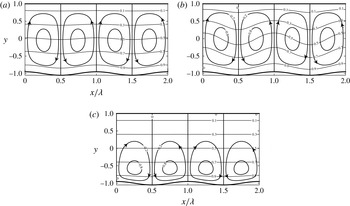
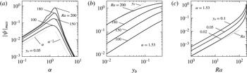
The rolls completely fill in the slot in the case of long corrugation wavelengths (see figure 3 a), the convection is very weak (see figure 4 a) and the temperature field modulations are relatively small. Reduction of the wavelength down to $\unicode[STIX]{x1D6FC}\approx 1$ results in the intensification of convection (see figure 4 a), with the rolls completely filling in the slot and significant modifications of the temperature field (see figure 3 b). Further reduction of the wavelength down to $\unicode[STIX]{x1D6FC}=5$ results in the weakening of convection (see figure 4 a), with the fluid movement as well as the temperature modifications concentrated in a boundary layer adjacent to the corrugated plate (see figure 3 c); the thickness of this boundary rapidly decreases with an increase of $\unicode[STIX]{x1D6FC}$ . The analysis carried out in § 3.1 shows that $|\unicode[STIX]{x1D713}|_{max}=O(\unicode[STIX]{x1D6FC})$ when $\unicode[STIX]{x1D6FC}\rightarrow 0$ , and the analysis carried out using the method described in Hossain & Floryan (Reference Hossain and Floryan2013a ,Reference Hossain and Floryan b , Reference Hossain and Floryan2015a ,Reference Hossain and Floryan b ) shows that $|\unicode[STIX]{x1D713}|_{max}=O(\unicode[STIX]{x1D6FC}^{-3})$ when $\unicode[STIX]{x1D6FC}\rightarrow \infty$ (details not given).

Figure 3.

The flow and temperature fields for $Ra=200$ , $y_{b}=0.05$ and $\unicode[STIX]{x1D6FC}=0.1$ (a), $\unicode[STIX]{x1D6FC}=1.53$ (b) and $\unicode[STIX]{x1D6FC}=5$ (c) normalized with their maxima; (a) $|\unicode[STIX]{x1D713}|_{max}=0.0149$ , (b) $|\unicode[STIX]{x1D713}|_{max}=0.7786$ , (c) $|\unicode[STIX]{x1D713}|_{max}=0.0040$ ; $\unicode[STIX]{x1D703}_{max}=Ra$ in all cases.

The effects of the remaining parameters can be deduced from the other data displayed in figure 4. An increase of $y_{b}$ results in an increase of $|\unicode[STIX]{x1D713}|_{max}$ initially proportional to $y_{b}$ , but slowing down for larger values of $y_{b}$ as the role of the plate shear increases (see figure 4 b). This slow-down occurs at smaller values of $y_{b}$ for larger values of $Ra$ . An increase of $Ra$ results in an increase of $|\unicode[STIX]{x1D713}|_{max}$ initially proportional to $Ra$ followed by a rapid acceleration for $Ra>100$ (see figure 4 c). This suggests that the system approaches a stability limit, as the critical value of the Rayleigh number in the case of smooth plates is $Ra_{cr}=213.5$ . The initial rate of growth of $|\unicode[STIX]{x1D713}|_{max}$ can be predicted analytically by linearizing the field equations using the weak-convection assumption (details not given; see Hossain, Floryan & Floryan Reference Hossain, Floryan and Floryan2012 and Floryan & Floryan Reference Floryan and Floryan2015).

Figure 4.

Variations of $|\unicode[STIX]{x1D713}|_{max}$ as a function of $\unicode[STIX]{x1D6FC}$ (a), $y_{b}$ (b) and $Ra$ (c). The thin dotted lines identify asymptotes.

Figure 5.

Variations of $\unicode[STIX]{x1D70E}_{t,L}$ , $\unicode[STIX]{x1D70E}_{t,U}$ (a) and $\unicode[STIX]{x1D70E}_{yp,L},\unicode[STIX]{x1D70E}_{yp,U}$ (b) for $y_{b}=0.05$ , $Ra=200$ , $C=0$ normalized with their maxima. The dotted, solid and dashed lines correspond to $\unicode[STIX]{x1D6FC}=0.1$ , 1.53, 5; $|\unicode[STIX]{x1D70E}_{t,L}|_{max}=0.1416$ , 6.8594, 0.3629; $|\unicode[STIX]{x1D70E}_{t,U}|_{max}=0.0947$ , 6.2586, 0.0041; $|\unicode[STIX]{x1D70E}_{yp,L}|_{max}=220.7034$ , 211.3108, 224.9411; $|\unicode[STIX]{x1D70E}_{yp,U}|_{max}=72.2485$ , 84.6565, 70.6266.

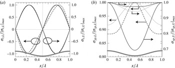
Variations of the forces acting on the two plates are illustrated in figure 5. The distribution of shear stresses is very similar for all $\unicode[STIX]{x1D6FC}$ values, i.e. they always act towards corrugation peaks, contributing to the potential corrugation build-up. 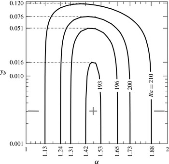The distribution of the $y$ component of pressure forces shows a qualitative change, with the maxima occurring at the corrugation troughs for small and large $\unicode[STIX]{x1D6FC}$ values but at the corrugation tips for medium $\unicode[STIX]{x1D6FC}$ values. The contours of $Dif_{1}=0$ displayed in figure 6 show that pressure may act in a manner consistent with corrugation build-up, but only if $Ra$ exceeds the critical value of 192.6, only for a certain finite range of $\unicode[STIX]{x1D6FC}$ values and only for a sufficiently small corrugation amplitude. Pressure always contributes to flattening of the corrugation if $Ra<192.6$ , $\unicode[STIX]{x1D6FC}$ values are either excessively small or excessively large and the amplitude is sufficiently large. In particular, pressure supports corrugation build-up for $Ra=193$ , 196, 200, 201 when $\unicode[STIX]{x1D6FC}\in (1.42,1.53)$ , (1.31, 1.65), (1.24, 1.73), (1.13, 1.88) and $y_{t}<0.016$ , 0.051, 0.076, 0.12 respectively. The $\unicode[STIX]{x1D6FC}$ intervals have been determined analytically using the small-amplitude solution described in appendix B.

Figure 6.

Contour plots of $Dif_{1}=0$ (see (3.4)) in the $(\unicode[STIX]{x1D6FC},y_{b})$ -plane.

Figure 7.

Variations of $Nu_{av}$ (a) and $Nu_{conv,av}/Nu_{av}$ (b) as functions of $\unicode[STIX]{x1D6FC}$ , variations of $Nu_{av}$ as a function of $y_{b}$ (c) and variations of $Nu_{conv,av}$ as a function of $Ra$ (d). The dashed lines correspond to $Nu_{cond,av}$ (such lines for all $y_{b}$ values overlap in (d)). The thin dotted lines identify asymptotes.

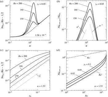
Changes of the heat transfer illustrated in figure 7(a) demonstrate the existence of a range of $\unicode[STIX]{x1D6FC}$ where convective effects play a role. To simplify interpretation, we represent the temperature field $\unicode[STIX]{x1D703}$ and the Nusselt number $Nu_{av}$ as a superposition of the conductive and convective components, i.e.

(3.6a,b )

$$\begin{eqnarray}\displaystyle \unicode[STIX]{x1D703}=\unicode[STIX]{x1D703}_{cond}+\unicode[STIX]{x1D703}_{conv},\quad Nu_{av}=Nu_{cond,av}+Nu_{conv,av}, & & \displaystyle\end{eqnarray}$$

where $\unicode[STIX]{x1D703}_{cond}$ represents the solution of the conduction problem (2.14) and $\unicode[STIX]{x1D703}_{conv}$ has been determined by subtracting $\unicode[STIX]{x1D703}_{cond}$ from $\unicode[STIX]{x1D703}$ . The conductive part has a well-known smooth-slot limit $Nu_{cond,av}\rightarrow Ra/2$ . Figure 7(a) illustrates variations of the excess heat flow above the smooth plate limit, i.e. $(Nu_{av}/Ra)-1/2$ , as a function of the wavenumber $\unicode[STIX]{x1D6FC}$ . When $\unicode[STIX]{x1D6FC}\rightarrow 0$ , the heat flow is a little higher than in the smooth slot, i.e.

(3.7)

$$\begin{eqnarray}\displaystyle \lim _{\unicode[STIX]{x1D6FC}\rightarrow 0}\left(\frac{Nu_{av}}{Ra}-\frac{1}{2}\right)=\frac{1}{2}\left\{\left[1-\left(\frac{y_{b}}{2}\right)^{2}\right]^{-1/2}-1\right\}\approx \frac{y_{b}}{16}^{2}\approx 1.56\times 10^{-4}, & & \displaystyle\end{eqnarray}$$

which is due to changes in conduction. The conductive heat flow increases with $\unicode[STIX]{x1D6FC}$ , but at $\unicode[STIX]{x1D6FC}\approx 0.4$ the convective flow begins to play a role. The convective heat flow peaks at $\unicode[STIX]{x1D6FC}\approx 1.53$ and then rapidly decreases, with the conductive effects being dominant again. They keep increasing with $\unicode[STIX]{x1D6FC}$ towards the upper limit, which corresponds to the heat flow in a slot whose height has been reduced by half of the corrugation amplitude, i.e. $\lim _{\unicode[STIX]{x1D6FC}\rightarrow \infty }Nu_{cond,av}=(Ra/(2-y_{b}))$ . The results displayed in figure 7(b) show that convective effects need to be accounted for only for medium $\unicode[STIX]{x1D6FC}$ values, as they decrease as $\unicode[STIX]{x1D6FC}^{4}$ when $\unicode[STIX]{x1D6FC}\rightarrow 0$ and as $\unicode[STIX]{x1D6FC}^{-7}$ when $\unicode[STIX]{x1D6FC}\rightarrow \infty$ . The results displayed in figure 7(c) demonstrate that $Nu_{av}$ increases proportionally to $y_{b}^{2}$ , but this growth slows down when the amplitude becomes excessively large (see figure 7 c). This slow-down is associated with the increase of the surface area exposed to shear due to the growth of the corrugation amplitude. 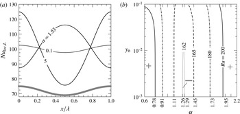The results displayed in figure 7(d) demonstrate that the convective heat flow increases proportionally to $Ra^{3}$ , with this growth rapidly accelerating when $Ra$ approaches the critical value for RB convection in the smooth slot. The variations of the local Nusselt number displayed in figure 8(a) demonstrate that the maxima of $Nu_{loc,L}$ occur at the corrugation peaks for small and large $\unicode[STIX]{x1D6FC}$ values but at the corrugation troughs for medium $\unicode[STIX]{x1D6FC}$ values. This effect is associated with a larger role of convective effects for medium $\unicode[STIX]{x1D6FC}$ values and their negligible role for large and small $\unicode[STIX]{x1D6FC}$ values. The changeover is well illustrated in figure 8(b), displaying variations of the difference $Dif_{2}$ between $Nu_{loc,L}$ at the peak and at the bottom of the trough, defined as

(3.8)

$$\begin{eqnarray}\displaystyle Dif_{2}=Nu_{loc,L}(0)-Nu_{loc,L}(\unicode[STIX]{x1D706}/2), & & \displaystyle\end{eqnarray}$$

as a function of $\unicode[STIX]{x1D6FC}$ and $y_{b}$ . The changeover may occur only if $Ra$ exceeds the critical value of 161.9, only in a finite range of $\unicode[STIX]{x1D6FC}$ values and only for a sufficiently small $y_{b}$ . Most of the heat flows through the corrugations peaks if $Ra$ is sufficiently small, $\unicode[STIX]{x1D6FC}$ values are either sufficiently small or sufficiently large and $y_{b}$ is sufficiently large. The range of $\unicode[STIX]{x1D6FC}$ when most of the heat flows through the corrugation troughs changes with $Ra$ , e.g. it is $\unicode[STIX]{x1D6FC}\in (1.26,1.29)$ , (1.11, 1.45), (0.91, 1.73), (0.78, 1.95) for $Ra=162$ , 165, 180, 200 respectively.

Figure 8.

Variations of $Nu_{loc,L}$ as a function of $x$ for $Ra=200$ , $y_{b}=0.05$ , $y_{t}=0$ , $\unicode[STIX]{x1D6FC}=0.1,1.53,5$ (a) and contour plots of $Dif_{2}=0$ (see (3.8)) in the ( $\unicode[STIX]{x1D6FC}$ , $y_{b}$ )-plane (b).

4 Corrugation at the upper plate

Corrugations placed on the upper plate produce convection analogous to that driven by corrugations placed on the lower plate. This similarity can be demonstrated by (i) reversing the direction of gravity, i.e. $Ra\rightarrow -Ra$ , and (ii) changing the sign of the temperature, i.e. $\unicode[STIX]{x1D703}\rightarrow -\unicode[STIX]{x1D703}$ (Hossain & Floryan Reference Hossain and Floryan2014).

5 Corrugations at both plates

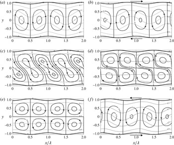
The patterns of motion displayed in figure 9 demonstrate a strong dependence on $\unicode[STIX]{x1D6FA}_{C}$ . Convection forms a single layer of rolls in the case of the ‘wavy slot’, with the fluid rising up above the peaks of the lower corrugation and flowing down above its troughs (see figure 9 a). As $\unicode[STIX]{x1D6FA}_{C}$ increases from 0 to $\unicode[STIX]{x03C0}$ , the rolls begin to deform, inflow stagnation points form in the middle of the slot and the rolls split into two layers when $\unicode[STIX]{x1D6FA}_{C}=\unicode[STIX]{x03C0}$ , with the slot assuming the ‘converging–diverging’ form. This transition is very rapid, as illustrated in figure 9(c–e), which displays flow topologies for $\unicode[STIX]{x1D6FA}_{C}=0.995\unicode[STIX]{x03C0}$ , $0.999\unicode[STIX]{x03C0}$ and $\unicode[STIX]{x03C0}$ . We shall begin detailed discussion with long-wavelength corrugations, i.e. with the limit $\unicode[STIX]{x1D6FC}\rightarrow 0$ .

Figure 9.

Flow and temperature fields for $\unicode[STIX]{x1D6FC}=1.53$ , $Ra=200$ , $y_{t}=y_{b}=0.05$ and (a) $\unicode[STIX]{x1D6FA}_{C}=0$ (the ‘wavy’ slot), (b) $\unicode[STIX]{x1D6FA}_{C}=\unicode[STIX]{x03C0}/2$ , (c) $\unicode[STIX]{x1D6FA}_{C}=0.995\unicode[STIX]{x03C0}$ , (d) $\unicode[STIX]{x1D6FA}_{C}=0.999\unicode[STIX]{x03C0}$ , (e) $\unicode[STIX]{x1D6FA}_{C}=\unicode[STIX]{x03C0}$ (the ‘converging–diverging’ slot), and (f) $\unicode[STIX]{x1D6FA}_{C}=3\unicode[STIX]{x03C0}/2$ . The maxima in (a–f) are $|\unicode[STIX]{x1D713}|_{max}=1.1696$ , 1.0709, 0.0232, 0.0179, 0.0173, 1.0709; $\unicode[STIX]{x1D703}_{max}=Ra$ in all cases.

5.1 Long-wavelength corrugation

A transformation of the form

(5.1a,b )

$$\begin{eqnarray}\displaystyle \unicode[STIX]{x1D709}=\unicode[STIX]{x1D6FC}x,\quad \unicode[STIX]{x1D702}=2\frac{y-1-y_{t}\cos (\unicode[STIX]{x1D709}+\unicode[STIX]{x1D6FA}_{C})}{2+y_{t}\cos (\unicode[STIX]{x1D709}+\unicode[STIX]{x1D6FA}_{C})-y_{b}\cos \unicode[STIX]{x1D709}}+1 & & \displaystyle\end{eqnarray}$$

maps the corrugated slot onto a regular strip $\unicode[STIX]{x1D702}\in [-1,1]$ and introduces the slow scale $\unicode[STIX]{x1D709}$ . Details of the solution are presented in appendix A. The forms of the $x$ components of the stresses as well as the tangential stresses acting on each plate, i.e.

(5.2a )

$$\begin{eqnarray}\displaystyle \unicode[STIX]{x1D70E}_{xv,L} & = & \displaystyle \unicode[STIX]{x1D70E}_{t,L}=-\unicode[STIX]{x1D6FC}\frac{Ra}{120Pr}\!\left\{\!L_{vL}+\!\mathop{\sum }_{n=1}^{2}[LS_{vL,n}\sin (n\unicode[STIX]{x1D709})+LC_{vL,n}\cos (n\unicode[STIX]{x1D709})]\right\}\!+O(\unicode[STIX]{x1D6FC}^{3}),\end{eqnarray}$$

(5.2b )

$$\begin{eqnarray}\displaystyle \unicode[STIX]{x1D70E}_{xv,U} & = & \displaystyle \unicode[STIX]{x1D70E}_{t,U}=\unicode[STIX]{x1D6FC}\frac{Ra}{120Pr}\!\left\{\!L_{vU}+\!\mathop{\sum }_{n=1}^{2}\!\left[LS_{vU,n}\sin (n\unicode[STIX]{x1D709})+LC_{vU,n}\cos (n\unicode[STIX]{x1D709})\right]\!\right\}\!+O(\unicode[STIX]{x1D6FC}^{3}),\end{eqnarray}$$

(5.2c )

$$\begin{eqnarray}\displaystyle \unicode[STIX]{x1D70E}_{xp,L} & = & \displaystyle \unicode[STIX]{x1D6FC}\left\{\frac{y_{b}Ra}{80Pr(2-y_{b}+y_{t}\cos \unicode[STIX]{x1D6FA}_{C})}\left\{L_{pL}+\mathop{\sum }_{n=1}^{2}\left[L_{pL,n}\sin (n\unicode[STIX]{x1D709})+LC_{pL,n}\cos (n\unicode[STIX]{x1D709})\right]\right\}\right.\nonumber\\ \displaystyle & & \displaystyle \left.-Cy_{b}\sin \unicode[STIX]{x1D709}\right\}+O(\unicode[STIX]{x1D6FC}^{2}),\end{eqnarray}$$

(5.2d )

$$\begin{eqnarray}\displaystyle \unicode[STIX]{x1D70E}_{xp,U} & = & \displaystyle \unicode[STIX]{x1D6FC}\left\{\frac{y_{t}Ra}{80Pr(2-y_{b}+y_{t}\cos \unicode[STIX]{x1D6FA}_{C})}\left\{L_{pU}+\mathop{\sum }_{n=1}^{2}\left[LS_{pU,n}\sin (n\unicode[STIX]{x1D709})+LC_{pU,n}\cos (n\unicode[STIX]{x1D709})\right]\right\}\right.\nonumber\\ \displaystyle & & \displaystyle \left.+\,Cy_{t}\sin (\unicode[STIX]{x1D709}+\unicode[STIX]{x1D6FA}_{C})\right\}+O(\unicode[STIX]{x1D6FC}^{2}),\end{eqnarray}$$

demonstrate the appearance of aperiodic terms which have interesting physical consequences discussed later in this presentation. Definitions of all coefficients used in (5.2) can be found in appendix A. It is instructive to rewrite (5.2) for

$y_{b}=y_{t}=S$ and three special

$\unicode[STIX]{x1D6FA}_{C}$ values whose significance will become obvious later in the discussion, i.e.

(5.3a,b )

$$\begin{eqnarray}\displaystyle \unicode[STIX]{x1D6FA}_{C}=0:\unicode[STIX]{x1D70E}_{t,L}=-\unicode[STIX]{x1D6FC}\frac{SRa}{6Pr}\sin \unicode[STIX]{x1D709},\quad \unicode[STIX]{x1D70E}_{t,U}=\unicode[STIX]{x1D6FC}\frac{SRa}{6Pr}\sin \unicode[STIX]{x1D709}, & & \displaystyle\end{eqnarray}$$

(5.3c )

$$\begin{eqnarray}\displaystyle \unicode[STIX]{x1D6FA}_{C}=\frac{\unicode[STIX]{x03C0}}{2}:\unicode[STIX]{x1D70E}_{t,L}=-\unicode[STIX]{x1D6FC}\frac{SRa}{120Pr}[12\sin \unicode[STIX]{x1D709}+8\cos \unicode[STIX]{x1D709}-5S\sin (2\unicode[STIX]{x1D709})+S\cos (2\unicode[STIX]{x1D709})-5S], & & \displaystyle\end{eqnarray}$$

(5.3d )

$$\begin{eqnarray}\displaystyle \unicode[STIX]{x1D70E}_{t,U}=\unicode[STIX]{x1D6FC}\frac{SRa}{120Pr}[8\sin \unicode[STIX]{x1D709}+12\cos \unicode[STIX]{x1D709}-5S\sin (2\unicode[STIX]{x1D709})-S\cos (2\unicode[STIX]{x1D709})-5S], & & \displaystyle\end{eqnarray}$$

(5.3e )

$$\begin{eqnarray}\displaystyle \unicode[STIX]{x1D6FA}_{C}=\unicode[STIX]{x03C0}:\unicode[STIX]{x1D70E}_{t,L}=-\unicode[STIX]{x1D6FC}\frac{SRa}{120Pr}[4\sin \unicode[STIX]{x1D709}-2S\sin (2\unicode[STIX]{x1D709})], & & \displaystyle\end{eqnarray}$$

(5.3f )

$$\begin{eqnarray}\displaystyle \unicode[STIX]{x1D70E}_{t,U}=-\unicode[STIX]{x1D6FC}\frac{SRa}{120Pr}[4\sin \unicode[STIX]{x1D709}-2S\sin (2\unicode[STIX]{x1D709})]. & & \displaystyle\end{eqnarray}$$

The total forces acting in the $x$ -direction per unit length of the slot can be determined as follows:

(5.4a )

$$\begin{eqnarray}\displaystyle F_{x,L} & = & \displaystyle F_{xv,L}+F_{xp,L}=\unicode[STIX]{x1D706}^{-1}\int _{0}^{\unicode[STIX]{x1D706}}\unicode[STIX]{x1D70E}_{xv,L}N_{L}^{-1}\,\text{d}x+\unicode[STIX]{x1D706}^{-1}\int _{0}^{\unicode[STIX]{x1D706}}\unicode[STIX]{x1D70E}_{xp,L}N_{L}^{-1}\,\text{d}x\nonumber\\ \displaystyle & = & \displaystyle +\unicode[STIX]{x1D6FC}\frac{y_{b}y_{t}Ra}{24Pr}\sin \unicode[STIX]{x1D6FA}_{C}-\unicode[STIX]{x1D6FC}\frac{3y_{b}y_{t}Ra}{40Pr}\sin \unicode[STIX]{x1D6FA}_{C}+O(\unicode[STIX]{x1D6FC}^{2})\nonumber\\ \displaystyle & = & \displaystyle -\unicode[STIX]{x1D6FC}\frac{y_{b}y_{t}Ra}{30Pr}\sin \unicode[STIX]{x1D6FA}_{C}+O(\unicode[STIX]{x1D6FC}^{2}),\end{eqnarray}$$

(5.4b )

$$\begin{eqnarray}\displaystyle F_{x,U} & = & \displaystyle F_{xv,U}+F_{xp,U}=\unicode[STIX]{x1D706}^{-1}\int _{0}^{\unicode[STIX]{x1D706}}\unicode[STIX]{x1D70E}_{xv,U}N_{U}^{-1}\,\text{d}x+\unicode[STIX]{x1D706}^{-1}\int _{0}^{\unicode[STIX]{x1D706}}\unicode[STIX]{x1D70E}_{xp,U}N_{U}^{-1}\,\text{d}x\nonumber\\ \displaystyle & = & \displaystyle -\unicode[STIX]{x1D6FC}\frac{y_{b}y_{t}Ra}{24Pr}\sin \unicode[STIX]{x1D6FA}_{C}+\unicode[STIX]{x1D6FC}\frac{3y_{b}y_{t}Ra}{40Pr}\sin \unicode[STIX]{x1D6FA}_{C}+O(\unicode[STIX]{x1D6FC}^{2})\nonumber\\ \displaystyle & = & \displaystyle \unicode[STIX]{x1D6FC}\frac{y_{b}y_{t}Ra}{30Pr}\sin \unicode[STIX]{x1D6FA}_{C}+O(\unicode[STIX]{x1D6FC}^{2}),\end{eqnarray}$$

where

$F_{x,L}$ and

$F_{x,U}$ denote the forces acting at the lower and upper plates respectively and

$F_{xv,L}$ ,

$F_{xv,U}$ and

$F_{xp,L}$ ,

$F_{xp,U}$ denote their viscous and pressure components respectively. The viscous and pressure forces do not balance out within one period as the aperiodic terms generate a net force, with pressure opposing shear and prevailing. The forces at the upper and lower plates are equal but act in opposite directions, producing a moment

(5.5)

$$\begin{eqnarray}\displaystyle M=2F_{x,U}=\unicode[STIX]{x1D6FC}\frac{y_{b}y_{t}Ra}{15Pr}\sin \unicode[STIX]{x1D6FA}_{C}+O(\unicode[STIX]{x1D6FC}^{2}), & & \displaystyle\end{eqnarray}$$

which attempts to change the relative positions of the plates. Positive $M$ corresponds to the upper plate being pushed to the right. Appearance of this moment correlates with loss of symmetry between the clockwise and anticlockwise rotations in the neighbouring cells (see figure 9). This dynamical system has two states of equilibrium defined by $M=0$ , i.e. the ‘wavy’ slot with $\unicode[STIX]{x1D6FA}_{C}=0$ and the ‘converging–diverging’ slot with $\unicode[STIX]{x1D6FA}_{C}=\unicode[STIX]{x03C0}$ . The second state is unstable as any small displacement from this position results in the formation of a moment that attempts to change the relative positions of the two plates until the ‘wavy’ configuration is achieved. The moment created by a single corrugation may be small, but a significant force may be created when many wavelengths are involved.

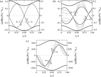
The shear stresses are directed towards the corrugation peaks, thus potentially contributing to the corrugation build-up (see figure 10). The stretching force acting on the plate has a periodic component, which changes direction within each corrugation half-wavelength, as well as an aperiodic component, which pulls the plate in the direction dictated by the phase shift $\unicode[STIX]{x1D6FA}_{C}$ . The periodic components of the stretching forces are defined as

(5.6a )

$$\begin{eqnarray}\displaystyle H_{t,L} & = & \displaystyle 2\unicode[STIX]{x1D706}^{-1}\int _{0}^{\unicode[STIX]{x1D706}/2}\unicode[STIX]{x1D70E}_{t,L}N_{L}^{-1}\,\text{d}x=-\unicode[STIX]{x1D6FC}\frac{Ra}{120\unicode[STIX]{x03C0}Pr}(24y_{b}+16y_{t}\cos \unicode[STIX]{x1D6FA}_{C}-5\unicode[STIX]{x03C0}y_{b}y_{t}\sin \unicode[STIX]{x1D6FA}_{C}),\nonumber\\ \displaystyle & & \displaystyle\end{eqnarray}$$

(5.6b )

$$\begin{eqnarray}\displaystyle H_{t,U} & = & \displaystyle 2\unicode[STIX]{x1D706}^{-1}\int _{(\unicode[STIX]{x1D706}/2)-(\unicode[STIX]{x1D6FA}_{C}/\unicode[STIX]{x1D6FC})}^{\unicode[STIX]{x1D706}-(\unicode[STIX]{x1D6FA}_{C}/\unicode[STIX]{x1D6FC})}\unicode[STIX]{x1D70E}_{t,U}N_{U}^{-1}\,\text{d}x\nonumber\\ \displaystyle & = & \displaystyle -\unicode[STIX]{x1D6FC}\frac{Ra}{120\unicode[STIX]{x03C0}Pr}(24y_{t}+16y_{b}\cos \unicode[STIX]{x1D6FA}_{C}+5\unicode[STIX]{x03C0}y_{b}y_{t}\sin \unicode[STIX]{x1D6FA}_{C}),\end{eqnarray}$$

and they assume the following values:

$H_{t,L}=-\unicode[STIX]{x1D6FC}(SRa/3\unicode[STIX]{x03C0}Pr)$ ,

$-\unicode[STIX]{x1D6FC}(SRa/120\unicode[STIX]{x03C0}Pr)(24-5\unicode[STIX]{x03C0}S)$ ,

$-\unicode[STIX]{x1D6FC}(SRa/15\unicode[STIX]{x03C0}Pr)$ and

$H_{t,U}=-\unicode[STIX]{x1D6FC}(SRa/3\unicode[STIX]{x03C0}Pr)$ ,

$-\unicode[STIX]{x1D6FC}(SRa/120\unicode[STIX]{x03C0}Pr)(24+5\unicode[STIX]{x03C0}S)$ ,

$-\unicode[STIX]{x1D6FC}(SRa/15\unicode[STIX]{x03C0}Pr)$ for

$\unicode[STIX]{x1D6FA}_{C}=0,\unicode[STIX]{x03C0}/2,\unicode[STIX]{x03C0}$ respectively.

Figure 10.

Distributions of $\unicode[STIX]{x1D70E}_{t,L}$ and $\unicode[STIX]{x1D70E}_{t,U}$ for $\unicode[STIX]{x1D6FA}_{C}=0$ (a), $\unicode[STIX]{x1D6FA}_{C}=\unicode[STIX]{x03C0}/2$ (b) and $\unicode[STIX]{x1D6FA}_{C}=\unicode[STIX]{x03C0}$ (c) for $Ra=200$ . The solid, dashed–dotted, dashed and dotted lines correspond to $y_{b}=y_{t}=S=0.05,0.1,0.5,1$ respectively. All lines overlap in (a). Lines corresponding to the lower and upper plates overlap in (c).

The forms of the $y$ components of forces acting on the plates, e.g.

(5.7a )

$$\begin{eqnarray}\displaystyle \left.\begin{array}{@{}c@{}}\unicode[STIX]{x1D70E}_{yv,L}=0(\unicode[STIX]{x1D6FC}^{2}),\\ \displaystyle \unicode[STIX]{x1D70E}_{yp,L}=\frac{Ra}{40Pr(2-y_{b}+y_{t}\cos \unicode[STIX]{x1D6FA}_{C})}(L_{1}\sin \unicode[STIX]{x1D709}+L_{2}\cos \unicode[STIX]{x1D709}+L_{3})+C+O(\unicode[STIX]{x1D6FC}^{2}),\end{array}\right\}\qquad & & \displaystyle\end{eqnarray}$$

(5.7b )

$$\begin{eqnarray}\displaystyle \left.\begin{array}{@{}c@{}}\unicode[STIX]{x1D70E}_{yv,U}=O(\unicode[STIX]{x1D6FC}^{2}),\\ \displaystyle \unicode[STIX]{x1D70E}_{yp,U}=-\frac{Ra}{40Pr(2-y_{b}+y_{t}\cos \unicode[STIX]{x1D6FA}_{C})}(L_{4}\sin \unicode[STIX]{x1D709}+L_{5}\cos \unicode[STIX]{x1D709}+L_{6})+C+O(\unicode[STIX]{x1D6FC}^{2}),\end{array}\right\}\qquad & & \displaystyle\end{eqnarray}$$

demonstrate the dominant role of pressure. Various coefficients used in (5.7) are defined in appendix A. To answer the question whether the pressure attempts to flatten corrugations, we compute the difference between the total pressure force acting on the part of the corrugation that bulges inwards, $H_{y,peak}$ , and on the part that bulges outwards, $H_{y,trough}$ . Such differences for the lower $(Dif_{1,L})$ and upper $(Dif_{1,U})$ plates are defined as follows:

(5.8a )

$$\begin{eqnarray}\displaystyle Dif_{1,L} & = & \displaystyle H_{y,peak,L}-H_{y,trough,L}\nonumber\\ \displaystyle & = & \displaystyle 2\unicode[STIX]{x1D706}^{-1}\int _{-\unicode[STIX]{x1D706}/4}^{\unicode[STIX]{x1D706}/4}(\unicode[STIX]{x1D70E}_{yp,L}+\unicode[STIX]{x1D70E}_{yv,L})\,\text{d}x-2\unicode[STIX]{x1D706}^{-1}\int _{\unicode[STIX]{x1D706}/4}^{3\unicode[STIX]{x1D706}/4}(\unicode[STIX]{x1D70E}_{yp,L}+\unicode[STIX]{x1D70E}_{yv,L})\,\text{d}x\nonumber\\ \displaystyle & = & \displaystyle -\frac{Ra}{20\unicode[STIX]{x03C0}Pr}(52y_{b}-12y_{t}\cos \unicode[STIX]{x1D6FA}_{C}),\end{eqnarray}$$

(5.8b )

$$\begin{eqnarray}\displaystyle Dif_{1,U} & = & \displaystyle H_{y,peak,U}-H_{y,trough,U}\nonumber\\ \displaystyle & = & \displaystyle 2\unicode[STIX]{x1D706}^{-1}\int _{(\unicode[STIX]{x1D706}/4)-(\unicode[STIX]{x1D6FA}_{C}/\unicode[STIX]{x1D6FC})}^{(3\unicode[STIX]{x1D706}/4)-(\unicode[STIX]{x1D6FA}_{C}/\unicode[STIX]{x1D6FC})}(\unicode[STIX]{x1D70E}_{yp,U}+\unicode[STIX]{x1D70E}_{yv,U})\,\text{d}x-2\unicode[STIX]{x1D706}^{-1}\int _{-(\unicode[STIX]{x1D706}/4)-(\unicode[STIX]{x1D6FA}_{C}/\unicode[STIX]{x1D6FC})}^{(\unicode[STIX]{x1D706}/4)-(\unicode[STIX]{x1D6FA}_{C}/\unicode[STIX]{x1D6FC})}(\unicode[STIX]{x1D70E}_{yp,U}+\unicode[STIX]{x1D70E}_{yv,U})\,\text{d}x\nonumber\\ \displaystyle & = & \displaystyle -\frac{Ra}{5\unicode[STIX]{x03C0}Pr}(7y_{t}+3y_{b}\cos \unicode[STIX]{x1D6FA}_{C}).\end{eqnarray}$$

Negative

$Dif_{1,L}$ and positive

$Dif_{1,U}$ imply flattening. When both corrugations have similar amplitudes, equation (5.8) shows that for long-wavelength corrugations pressure always contributes to flattening of the lower and build-up of the upper corrugations.

The local and average Nusselt numbers can be expressed as

(5.9)

$$\begin{eqnarray}\displaystyle \left.\begin{array}{@{}c@{}}\displaystyle Nu_{loc,L}=Nu_{loc,U}=\frac{Ra}{2+y_{t}\cos (\unicode[STIX]{x1D709}+\unicode[STIX]{x1D6FA}_{C})-y_{b}\cos \unicode[STIX]{x1D709}}+O(\unicode[STIX]{x1D6FC}^{2}),\\ \displaystyle Nu_{av}=\frac{Ra}{\sqrt{4-y_{b}^{2}-y_{t}^{2}+2y_{b}y_{t}\cos \unicode[STIX]{x1D6FA}_{C}}}+O(\unicode[STIX]{x1D6FC}^{2}).\end{array}\right\} & & \displaystyle\end{eqnarray}$$

The ratio $R$ of $Nu_{av}$ values for slots with both and single plates being corrugated, e.g.

(5.10)

$$\begin{eqnarray}\displaystyle R=\sqrt{\frac{4-y_{b}^{2}}{4-y_{b}^{2}-y_{t}^{2}+2y_{b}y_{t}\cos \unicode[STIX]{x1D6FA}_{C}}}, & & \displaystyle\end{eqnarray}$$

shows that the heat transfer is increased by adding the upper corrugation only when $\cos \unicode[STIX]{x1D6FA}_{C}<y_{t}/2y_{b}$ . In the case of equal amplitudes, the heat transfer is increased when $\unicode[STIX]{x03C0}/3<\unicode[STIX]{x1D6FA}_{C}<5\unicode[STIX]{x03C0}/3$ . This suggests a possible use of the positioning of the upper corrugation as a heat transfer control device, as one can significantly increase/decrease the heat flow by simply changing the phase shift.

5.2 Corrugations with an arbitrary wavenumber

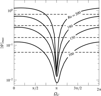
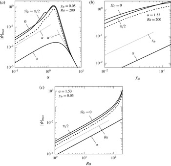
The discussion presented in the previous section demonstrates that the phase shift $\unicode[STIX]{x1D6FA}_{C}$ is a very strong parameter. The convection intensity may change by an order of magnitude when $\unicode[STIX]{x1D6FA}_{C}$ changes from 0 to $\unicode[STIX]{x03C0}$ , as illustrated in figure 11. The most intense motion occurs at $\unicode[STIX]{x1D6FC}\approx 1.53$ and it rapidly decreases for both smaller and larger $\unicode[STIX]{x1D6FC}$ values (see figure 12 a). The asymptotes do not depend on $\unicode[STIX]{x1D6FA}_{C}$ and are $|\unicode[STIX]{x1D713}|_{max}=O(\unicode[STIX]{x1D6FC})$ when $\unicode[STIX]{x1D6FC}\rightarrow 0$ and $|\unicode[STIX]{x1D713}|_{max}=O(\unicode[STIX]{x1D6FC}^{-3})$ when $\unicode[STIX]{x1D6FC}\rightarrow \infty$ , i.e. they are the same as for convection in a slot with one corrugated plate. The value of $|\unicode[STIX]{x1D713}|_{max}$ increases initially proportionally to the amplitude of the corrugation, as shown in figure 12(b), until increase of the length of the plates combined with shear slows it down. This slow-down occurs at the smallest amplitudes for $\unicode[STIX]{x1D6FA}_{C}\approx 0$ , i.e. when the convection is most intense. The intensity increases proportionally to $Ra$ but, when $Ra$ approaches the critical value associated with RB convection, its growth rapidly accelerates (see figure 12 c). The most rapid acceleration is observed for $\unicode[STIX]{x1D6FA}_{C}\approx \unicode[STIX]{x03C0}/2$ .

Figure 11.

Variations of $|\unicode[STIX]{x1D713}|_{max}$ as a function of $\unicode[STIX]{x1D6FA}_{C}$ for $y_{b}=y_{t}=0.05$ and $\unicode[STIX]{x1D6FC}=1.53$ . The dashed lines correspond to corrugations removed from the upper plate.

Figure 12.

Variations of $|\unicode[STIX]{x1D713}|_{max}$ as a function of $\unicode[STIX]{x1D6FC}$ (a), $y_{tb}=y_{t}=y_{b}$ (b) and $Ra$ (c). The dashed lines correspond to corrugations removed from the upper plate. The thin dotted lines identify asymptotes.

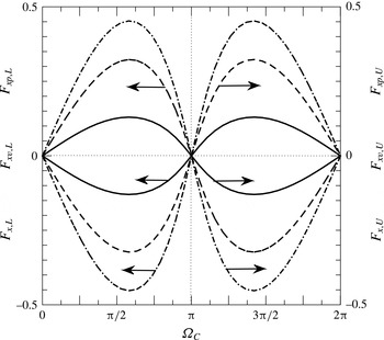
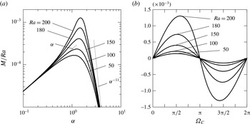
The variations of forces acting at both plates as functions of $\unicode[STIX]{x1D6FA}_{C}$ illustrated in figure 13 demonstrate that their maxima occur for $\unicode[STIX]{x1D6FA}_{C}\approx 7\unicode[STIX]{x03C0}/12$ and $17\unicode[STIX]{x03C0}/12$ , the pressure force always opposes the viscous force and, since it is much stronger, it determines the direction of the total force. The results presented in figure 14(a) demonstrate that the moment $M$ changes rapidly as a function of the corrugation wavenumber, with the largest magnitude attained for $\unicode[STIX]{x1D6FC}\approx 1.5$ , and this magnitude rapidly increases with $Ra$ . Use of corrugations with smaller wavenumbers reduces $M$ proportionally to $\unicode[STIX]{x1D6FC}$ , and use of larger $\unicode[STIX]{x1D6FC}$ values reduces $M$ proportionally to $\unicode[STIX]{x1D6FC}^{-11}$ . Figure 14(b) demonstrates that $M$ is positive for $\unicode[STIX]{x1D6FA}_{C}\in (0,\unicode[STIX]{x03C0})$ and negative for $\unicode[STIX]{x1D6FA}_{C}\in (\unicode[STIX]{x03C0},2\unicode[STIX]{x03C0})$ , it changes smoothly in the whole range of $\unicode[STIX]{x1D6FA}_{C}$ , the maxima of $|M|$ occur at $\unicode[STIX]{x1D6FA}_{C}\approx 7\unicode[STIX]{x03C0}/12$ and $17\unicode[STIX]{x03C0}/12$ , and the zeros correspond to the two special points, i.e. to $\unicode[STIX]{x1D6FA}_{C}=0,\unicode[STIX]{x03C0}$ .

Figure 13.

Variations of $F_{xv,L}$ and $F_{xv,U}$ (dashed lines), $F_{xp,L}$ and $F_{xp,U}$ (dashed–dotted lines), and $F_{x,L}$ and $F_{x,U}$ (solid lines) as functions of $\unicode[STIX]{x1D6FA}_{C}$ for $\unicode[STIX]{x1D6FC}=1.53$ , $Ra=200,y_{t}=y_{b}=0.05$ .

Figure 14.

Variations of $M$ as a function of $\unicode[STIX]{x1D6FC}$ for $\unicode[STIX]{x1D6FA}_{C}=\unicode[STIX]{x03C0}/2$ (a) and as a function of $\unicode[STIX]{x1D6FA}_{C}$ for $\unicode[STIX]{x1D6FC}=1.49$ (b) for $y_{t}=y_{b}=0.05$ . The thin dotted lines identify asymptotes.

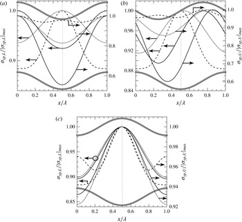
The distributions of tangential stresses are similar for all $\unicode[STIX]{x1D6FC}$ and $\unicode[STIX]{x1D6FA}_{C}$ values, with shear always directed towards the corrugation peak and, thus, potentially contributing to the corrugation build-up. The distributions of pressure forces have different forms at the lower and upper plates (figure 15). At the lower plate, pressure maxima generally occur at the corrugation troughs except for medium $\unicode[STIX]{x1D6FC}$ values where the maxima occur at the corrugation peaks, but only if the phase difference is not too close to $\unicode[STIX]{x1D6FA}_{C}=\unicode[STIX]{x03C0}$ , while at the upper plate the maxima always occur in the troughs. 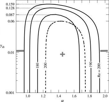The net effect of pressure forces can be assessed by evaluating $Dif_{1,L}$ and $Dif_{1,U}$ (see (5.8)). Pressure contributes to the corrugation build-up at the lower plate when $Dif_{1,L}>0$ , and this occurs only for a finite range of medium $\unicode[STIX]{x1D6FC}$ values, for $Ra$ values that are large enough and for corrugation amplitudes that are small enough (figure 16). At the upper plate, pressure forces would always contribute to the corrugation build-up as $Dif_{1,U}$ is always negative.

Figure 15.

Variations of $\unicode[STIX]{x1D70E}_{yp,L}$ and $\unicode[STIX]{x1D70E}_{yp,U}$ as functions of $x$ for $Ra=200$ , $y_{b}=y_{t}=0.05$ , $\unicode[STIX]{x1D6FC}=0.1$ (dotted lines), $\unicode[STIX]{x1D6FC}=1.53$ (solid lines) and $\unicode[STIX]{x1D6FC}=5$ (dashed lines) for $\unicode[STIX]{x1D6FA}_{C}=0$ (a), $\unicode[STIX]{x1D6FA}_{C}=\unicode[STIX]{x03C0}/2$ (b) and $\unicode[STIX]{x1D6FA}_{C}=\unicode[STIX]{x03C0}$ (c).

Figure 16.

Contour plots of $Dif_{1,L}=0$ (see (5.8)) in the ( $\unicode[STIX]{x1D6FC}$ , $y_{tb}$ )-plane for $y_{t}=y_{b}=y_{tb}$ and $\unicode[STIX]{x1D6FA}_{C}=0$ , $\unicode[STIX]{x03C0}$ (solid and dashed lines respectively).

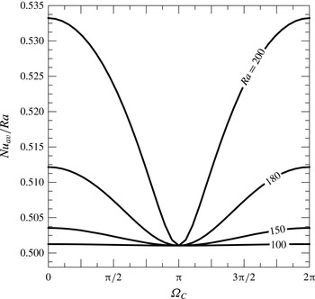
The Nusselt number strongly depends on $\unicode[STIX]{x1D6FA}_{C}$ , with the largest heat flow corresponding to the ‘wavy’ configuration $(\unicode[STIX]{x1D6FA}_{C}=0)$ and the smallest corresponding to the ‘converging–diverging’ configuration $(\unicode[STIX]{x1D6FA}_{C}=\unicode[STIX]{x03C0})$ , as illustrated in figure 17. The range of variations of $Nu_{av}$ increases significantly with an increase of $Ra$ (see figure 17).

Figure 17.

Variations of $Nu_{av}$ as a function of $\unicode[STIX]{x1D6FA}_{C}$ for $y_{t}=y_{b}=0.05,\unicode[STIX]{x1D6FC}=1.53$ .

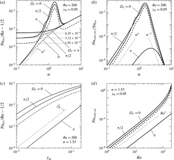
The discussion of $Nu_{av}$ dependence on the slot geometry starts with the smooth-slot limit, i.e. $y_{t}\rightarrow 0$ , $y_{b}\rightarrow 0$ , $Nu_{av}\rightarrow Ra/2$ . Figure 18(a) illustrates variations of the heat transfer augmentation, i.e. increase of the heat flow above this limit. Its form for $\unicode[STIX]{x1D6FC}\rightarrow 0$ (see § 5.1), i.e.

(5.11)

$$\begin{eqnarray}\displaystyle \lim _{\unicode[STIX]{x1D6FC}\rightarrow 0}\left(\frac{Nu_{av}}{Ra}-\frac{1}{2}\right) & = & \displaystyle \frac{1}{2}\left\{\left[1-\left(\frac{y_{b}}{2}\right)^{2}-\left(\frac{y_{t}}{2}\right)^{2}+\frac{y_{b}y_{t}\cos \unicode[STIX]{x1D6FA}_{C}}{2}\right]^{-1/2}-1\right\}\nonumber\\ \displaystyle & {\approx} & \displaystyle \frac{y_{b}^{2}+y_{t}^{2}-2y_{b}y_{t}\cos \unicode[STIX]{x1D6FA}_{C}}{16},\end{eqnarray}$$

demonstrates a strong dependence of this augmentation on $\unicode[STIX]{x1D6FA}_{C}$ . To illustrate this point, (5.11) is evaluated for $y_{b}=y_{t}$ and typical $\unicode[STIX]{x1D6FA}_{C}$ values, i.e.

(5.12)

$$\begin{eqnarray}\displaystyle \left.\begin{array}{@{}c@{}}\displaystyle \unicode[STIX]{x1D6FA}_{C}=0:\quad \frac{Nu_{av}}{Ra}-\frac{1}{2}\approx \frac{(y_{b}-y_{t})^{2}}{16}=0,\\ \displaystyle \unicode[STIX]{x1D6FA}_{C}=\unicode[STIX]{x03C0}/2:\quad \frac{Nu_{av}}{Ra}-\frac{1}{2}\approx \frac{y_{b}^{2}+y_{t}^{2}}{16}=\frac{y_{b}^{2}}{8}=3.12\times 10^{-4},\\ \displaystyle \unicode[STIX]{x1D6FA}_{C}=\unicode[STIX]{x03C0}:\quad \frac{Nu_{av}}{Ra}-\frac{1}{2}\approx \frac{(y_{b}+y_{t})^{2}}{16}=\frac{y_{b}^{2}}{4}=6.25\times 10^{-4}.\end{array}\right\} & & \displaystyle\end{eqnarray}$$

The above relations show that the heat transfer can be either larger than or equal to the smooth-slot limit depending on the phase difference. Figure 18(a) shows that $(Nu_{av}/Ra)-(1/2)$ either approaches an amplitude-dependent constant or decreases to zero as $\unicode[STIX]{x1D6FC}\rightarrow 0$ depending on $\unicode[STIX]{x1D6FA}_{C}$ . An increase of $\unicode[STIX]{x1D6FC}$ increases the heat flow mainly due to an increase of the corrugation-driven conduction heat flow. At $\unicode[STIX]{x1D6FC}\approx 0.4$ , convective effects begin to play a role and the heat flow increases above that expected from the pure conduction, but only if $\unicode[STIX]{x1D6FA}_{C}$ is not too close to $\unicode[STIX]{x03C0}$ , as convective effects play almost no role for the ‘converging–diverging’ configuration. The convective effects peak at $\unicode[STIX]{x1D6FC}\approx 1.53$ for all $\unicode[STIX]{x1D6FA}_{C}$ values that are not too close to $\unicode[STIX]{x03C0}$ and then they rapidly decrease with a further increase of $\unicode[STIX]{x1D6FC}$ , with the heat flow being again dominated by the conduction and with its increase resulting from the corrugation-driven changes in the conduction. The upper limit on this growth corresponds to conduction in a slot whose height has been reduced by half of the corrugation amplitude, i.e. $\lim _{\unicode[STIX]{x1D6FC}\rightarrow \infty }Nu_{cond,av}=(Ra/(2-y_{b}-y_{t}))$ . The variations of the convective effects are well illustrated in figure 18(b). These effects need to be accounted only for $\unicode[STIX]{x1D6FA}_{C}$ values that are not too close to $\unicode[STIX]{x03C0}$ and only for a range of medium $\unicode[STIX]{x1D6FC}$ values. Figure 18(c) demonstrates that $Nu_{av}$ increases away from the smooth-slot limit proportionally to $y_{tb}^{2}$ for all $\unicode[STIX]{x1D6FA}_{C}$ values, with $Nu_{av}$ for $\unicode[STIX]{x1D6FA}_{C}\approx \unicode[STIX]{x03C0}$ being at least two orders of magnitude smaller than $Nu_{av}$ for $\unicode[STIX]{x1D6FA}_{C}\approx 0$ . This growth begins to slow down when the amplitude becomes excessively large, as illustrated in figure 18(c), with the earliest slow-down occurring for $\unicode[STIX]{x1D6FA}_{C}\approx 0$ , which corresponds to the strongest convection. The convective heat flow increases proportionally to $Ra^{3}$ , with this growth rapidly accelerating when $Ra$ approaches the critical value, giving rise to transition to a secondary state in a smooth slot (see figure 18 d).

Figure 18.

Variations of $Nu_{av}$ (a) and $Nu_{conv,av}/Nu_{av}$ (b) as functions of $\unicode[STIX]{x1D6FC}$ , variation of $Nu_{av}$ as a function of $y_{tb}=y_{b}=y_{t}$ (c) and variation of $Nu_{conv,av}$ as a function of $Ra$ (d). The dashed lines correspond to corrugations removed from the upper plate. The dashed–dotted lines in (a) describe $Nu_{cond,av}$ (the dashed–dotted and solid lines overlap for $\unicode[STIX]{x1D6FA}_{C}=\unicode[STIX]{x03C0}$ ). The thin dotted lines identify asymptotes.

6 Effects of Prandtl number

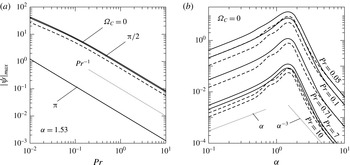
The results presented in the previous sections have been obtained for $Pr=0.71$ . As convection is driven by the horizontal temperature gradients, which are dominated by conductive effects, one should expect an increase of convection intensity as $Pr$ is reduced. The results displayed in figure 19(a) confirm this prediction. 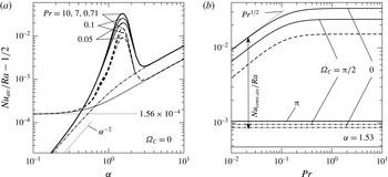The most intense convection occurs for $\unicode[STIX]{x1D6FC}\approx 1.53$ , and it decreases for $\unicode[STIX]{x1D6FC}\rightarrow 0$ and $\unicode[STIX]{x1D6FC}\rightarrow \infty$ always in the same manner regardless of the value of $Pr$ , as illustrated in figure 19(b). The heat transfer process displays the same characteristics, with conduction dominating its increase above the smooth-slot limit for both small and large $\unicode[STIX]{x1D6FC}$ values and convection dominating this increase for $\unicode[STIX]{x1D6FC}=O(1)$ , as illustrated in figure 20(a). The increase of $Pr$ leads to larger convective corrections as convective transport becomes stronger than the conductive transport. This process is well illustrated in figure 20(b), displaying variation of $Nu_{av}$ as a function of $Pr$ . The convective part becomes stronger as $Pr$ increases and reaches the limiting state for $Pr>1$ .

Figure 19.

Variations of $|\unicode[STIX]{x1D713}|_{max}$ as a function of $Pr$ (a) and $\unicode[STIX]{x1D6FC}$ (b) for $y_{t}=y_{b}=0.05$ , $Ra=200$ . The dashed lines correspond to corrugations removed from the upper plate. The thin dotted lines identify asymptotes.

Figure 20.

Variations of $Nu_{av}$ as functions of $Pr$ and $\unicode[STIX]{x1D6FC}$ for $y_{t}=y_{b}=0.05$ and $Ra=200$ . Variations of $Nu_{cond,av}$ are illustrated using dashed–dotted lines. Variations of $Nu_{av}$ and $Nu_{cond,av}$ for the upper corrugations removed are illustrated using dashed and dotted lines respectively. The lines for $Nu_{av}$ and $Nu_{cond,av}$ overlap in (b) when $\unicode[STIX]{x1D6FA}_{C}=\unicode[STIX]{x03C0}$ . The thin dotted lines identify asymptotes.

7 Conclusions

Analysis of natural convection in a horizontal slot formed by two corrugated isothermal plates has been carried out for subcritical Rayleigh numbers $Ra$ . The corrugations have sinusoidal form and can be placed either at one or at both plates, with their geometry described by the wavenumber $\unicode[STIX]{x1D6FC}$ , the upper $y_{t}$ and lower $y_{b}$ amplitudes and the phase shift $\unicode[STIX]{x1D6FA}_{c}$ between the upper and lower corrugation systems. The corrugations create horizontal temperature gradients which lead to the formation of vertical and horizontal pressure gradients which drive the motion for any $Ra$ . The convection rolls have their size dictated by the corrugation wavelength and fill in the slot completely except for short-wavelength corrugations where the motion is confined to a boundary layer adjacent to the corrugated plate.

The most intense convection when corrugation is placed at the lower plate occurs for $\unicode[STIX]{x1D6FC}\approx 1.53$ regardless of $Ra$ , $Pr$ and the amplitudes. Its intensity initially increases proportionally to $Ra$ but then rapidly accelerates when $Ra$ approaches conditions giving rise to secondary flows in smooth slots. It also increases proportionally to the amplitude, but the growth slows down when an excessively large amplitude is reached. Transfer of the corrugations to the upper plate results in a similar convection. Placement of corrugations at both plates may either significantly increase or decrease convection depending on $\unicode[STIX]{x1D6FA}_{c}$ . The most intense convection occurs for $\unicode[STIX]{x1D6FA}_{c}=0$ (‘wavy’ slot) and is almost twice as strong as convection driven by corrugation at one plate, and the weakest convection corresponds to $\unicode[STIX]{x1D6FA}_{c}=\unicode[STIX]{x03C0}$ (‘converging–diverging’ slot). The latter convection is very weak and has no practical significance. Reduction of $Pr$ increases the strength of convection proportionally to $Pr^{-1}$ .

The shear forces created by convection act in a manner consistent with corrugation build-up, while the role of the pressure forces depends on the corrugation geometry, its location at either the lower or the upper plate and the Rayleigh number. When the upper plate is corrugated, pressure always contributes to flattening. When the lower plate is corrugated, pressure generally contributes to flattening except for a range of $\unicode[STIX]{x1D6FC}=O(1)$ combined with a sufficiently small corrugation amplitude and with a sufficiently large $Ra$ . Build-up of the corrugations is likely to occur under such conditions as both the pressure and the shear act in the same manner. When both plates are corrugated, the horizontal forces create a moment which attempts to change their relative position. There are two states of equilibrium corresponding to elimination of this moment, i.e. the ‘wavy’ slot and the ‘converging–diverging’ slot. The latter is unstable as small departures from this state create a moment that attempts to change the relative position of the plates until the ‘wavy’ configuration is reached.

The presence of corrugations changes the conductive state and creates convective heat flows. The former increases with an increase of $\unicode[STIX]{x1D6FC}$ , but this growth is limited from above by conduction in a smooth slot whose height is reduced by half of the corrugation amplitude. The latter is relevant only for $\unicode[STIX]{x1D6FC}=O(1)$ , with $\unicode[STIX]{x1D6FC}\approx 1.53$ producing the largest heat flow. The heat flow changes by an order of magnitude depending on $\unicode[STIX]{x1D6FA}_{C}$ , with the maxima and minima occurring in the ‘wavy’ and ‘converging–diverging’ slots respectively.

The corrugation-induced convection is expected to go through a transition to a secondary convection. The form of this convection as well as the onset conditions remain to be determined.

Acknowledgement

This work has been carried out with the support of NSERC of Canada.

Appendix A. Solution for long-wavelength corrugations $(\unicode[STIX]{x1D6FC}\rightarrow 0)$ placed at both plates

A transformation of the form

(A 1a,b )

maps the corrugated slot onto a regular strip $\unicode[STIX]{x1D702}\in [-1,1]$ and introduces the slow scale $\unicode[STIX]{x1D709}$ . Simplified solutions for corrugations placed at either the lower or the upper plate can be found by taking limits of either $y_{t}\rightarrow 0$ or $y_{b}\rightarrow 0$ respectively. The field equations expressed in ( $\unicode[STIX]{x1D709}$ , $\unicode[STIX]{x1D702}$ )-coordinates have the following form:

(A 2a )

$$\begin{eqnarray}\displaystyle & \displaystyle \unicode[STIX]{x1D6FC}\frac{\unicode[STIX]{x2202}u}{\unicode[STIX]{x2202}\unicode[STIX]{x1D709}}+F_{7}\frac{\unicode[STIX]{x2202}u}{\unicode[STIX]{x2202}\unicode[STIX]{x1D702}}+F_{8}\frac{\unicode[STIX]{x2202}v}{\unicode[STIX]{x2202}\unicode[STIX]{x1D702}}=0, & \displaystyle\end{eqnarray}$$

(A 2b )

$$\begin{eqnarray}\displaystyle & \displaystyle \frac{\unicode[STIX]{x2202}^{2}u}{\unicode[STIX]{x2202}\unicode[STIX]{x1D702}^{2}}+[F_{1}-F_{2}u-F_{3}v]\frac{\unicode[STIX]{x2202}u}{\unicode[STIX]{x2202}\unicode[STIX]{x1D702}}+F_{4}\frac{\unicode[STIX]{x2202}^{2}u}{\unicode[STIX]{x2202}\unicode[STIX]{x1D709}\unicode[STIX]{x2202}\unicode[STIX]{x1D702}}+F_{5}\frac{\unicode[STIX]{x2202}^{2}u}{\unicode[STIX]{x2202}\unicode[STIX]{x1D709}^{2}}-F_{6}u\frac{\unicode[STIX]{x2202}u}{\unicode[STIX]{x2202}\unicode[STIX]{x1D709}}-F_{6}\frac{\unicode[STIX]{x2202}p}{\unicode[STIX]{x2202}\unicode[STIX]{x1D709}}-F_{2}\frac{\unicode[STIX]{x2202}p}{\unicode[STIX]{x2202}\unicode[STIX]{x1D702}}=0, & \displaystyle \nonumber\\ \displaystyle & & \displaystyle\end{eqnarray}$$

(A 2c )

$$\begin{eqnarray}\displaystyle & \displaystyle \frac{\unicode[STIX]{x2202}^{2}v}{\unicode[STIX]{x2202}\unicode[STIX]{x1D702}^{2}}+[F_{1}-F_{2}u-F_{3}v]\frac{\unicode[STIX]{x2202}v}{\unicode[STIX]{x2202}\unicode[STIX]{x1D702}}+F_{4}\frac{\unicode[STIX]{x2202}^{2}v}{\unicode[STIX]{x2202}\unicode[STIX]{x1D709}\unicode[STIX]{x2202}\unicode[STIX]{x1D702}}+F_{5}\frac{\unicode[STIX]{x2202}^{2}v}{\unicode[STIX]{x2202}\unicode[STIX]{x1D709}^{2}}-F_{6}u\frac{\unicode[STIX]{x2202}v}{\unicode[STIX]{x2202}\unicode[STIX]{x1D709}}-F_{3}\frac{\unicode[STIX]{x2202}p}{\unicode[STIX]{x2202}\unicode[STIX]{x1D702}}+Pr^{-1}F_{9}\unicode[STIX]{x1D703}=0, & \displaystyle \nonumber\\ \displaystyle & & \displaystyle\end{eqnarray}$$

(A 2d )

$$\begin{eqnarray}\displaystyle & \displaystyle \frac{\unicode[STIX]{x2202}^{2}\unicode[STIX]{x1D703}}{\unicode[STIX]{x2202}\unicode[STIX]{x1D702}^{2}}+[F_{1}-PrF_{2}u-PrF_{3}v]\frac{\unicode[STIX]{x2202}\unicode[STIX]{x1D703}}{\unicode[STIX]{x2202}\unicode[STIX]{x1D702}}+F_{4}\frac{\unicode[STIX]{x2202}^{2}\unicode[STIX]{x1D703}}{\unicode[STIX]{x2202}\unicode[STIX]{x1D709}\unicode[STIX]{x2202}\unicode[STIX]{x1D702}}+F_{5}\frac{\unicode[STIX]{x2202}^{2}\unicode[STIX]{x1D703}}{\unicode[STIX]{x2202}\unicode[STIX]{x1D709}^{2}}-PrF_{6}u\frac{\unicode[STIX]{x2202}\unicode[STIX]{x1D703}}{\unicode[STIX]{x2202}\unicode[STIX]{x1D709}}=0, & \displaystyle\end{eqnarray}$$

where

(A 3)

$$\begin{eqnarray}\displaystyle \left.\begin{array}{@{}c@{}}\displaystyle F_{1}=\frac{\unicode[STIX]{x1D702}_{xx}}{\unicode[STIX]{x1D702}_{x}^{2}+\unicode[STIX]{x1D702}_{y}^{2}}=\unicode[STIX]{x1D6FC}^{2}\frac{(2M_{3}^{2}+M_{1}G)\unicode[STIX]{x1D702}+M_{2}G+2M_{3}M_{4}}{4}+O(\unicode[STIX]{x1D6FC}^{4}),\\ \displaystyle F_{2}=\frac{\unicode[STIX]{x1D702}_{x}}{\unicode[STIX]{x1D702}_{x}^{2}+\unicode[STIX]{x1D702}_{y}^{2}}=\unicode[STIX]{x1D6FC}\frac{G(M_{3}\unicode[STIX]{x1D702}+M_{4})}{4}+O(\unicode[STIX]{x1D6FC}^{3}),\\ \displaystyle F_{3}=\frac{\unicode[STIX]{x1D702}_{y}}{\unicode[STIX]{x1D702}_{x}^{2}+\unicode[STIX]{x1D702}_{y}^{2}}=\frac{G}{2}-\unicode[STIX]{x1D6FC}^{2}\frac{G(M_{3}\unicode[STIX]{x1D702}+M_{4})^{2}}{8}+O(\unicode[STIX]{x1D6FC}^{4}),\quad F_{4}=\frac{2\unicode[STIX]{x1D6FC}\unicode[STIX]{x1D702}_{x}}{\unicode[STIX]{x1D702}_{x}^{2}+\unicode[STIX]{x1D702}_{y}^{2}}=2\unicode[STIX]{x1D6FC}F_{2},\\ \displaystyle F_{5}=\frac{\unicode[STIX]{x1D6FC}^{2}}{\unicode[STIX]{x1D702}_{x}^{2}+\unicode[STIX]{x1D702}_{y}^{2}}=\unicode[STIX]{x1D6FC}F_{6},\\ \displaystyle F_{6}=\frac{\unicode[STIX]{x1D6FC}}{\unicode[STIX]{x1D702}_{x}^{2}+\unicode[STIX]{x1D702}_{y}^{2}}=\unicode[STIX]{x1D6FC}\frac{G^{2}}{4}+O(\unicode[STIX]{x1D6FC}^{3}),\quad F_{7}=\unicode[STIX]{x1D702}_{x}=\unicode[STIX]{x1D6FC}\frac{M_{3}\unicode[STIX]{x1D702}+M_{4}}{G},\quad F_{8}=\unicode[STIX]{x1D702}_{y}=\frac{2}{G},\\ \displaystyle F_{9}=\frac{1}{\unicode[STIX]{x1D702}_{x}^{2}+\unicode[STIX]{x1D702}_{y}^{2}}=\frac{G^{2}}{4}-\unicode[STIX]{x1D6FC}^{2}\frac{G^{2}(M_{3}\unicode[STIX]{x1D702}+M_{4})^{2}}{16}+O(\unicode[STIX]{x1D6FC}^{4}),\\ \displaystyle G=2+M_{1},\quad M_{1}=y_{t}\cos (\unicode[STIX]{x1D709}+\unicode[STIX]{x1D6FA}_{C})-y_{b}\cos \unicode[STIX]{x1D709},\\ \displaystyle M_{2}=y_{t}\cos (\unicode[STIX]{x1D709}+\unicode[STIX]{x1D6FA}_{C})+y_{b}\cos \unicode[STIX]{x1D709},\\ \displaystyle M_{3}=y_{t}\sin (\unicode[STIX]{x1D709}+\unicode[STIX]{x1D6FA}_{C})-y_{b}\sin \unicode[STIX]{x1D709},\quad M_{4}=y_{t}\sin (\unicode[STIX]{x1D709}+\unicode[STIX]{x1D6FA}_{C})+y_{b}\sin \unicode[STIX]{x1D709},\end{array}\right\} & & \displaystyle\end{eqnarray}$$

and are subject to the following boundary conditions:

(A 4a-d )

$$\begin{eqnarray}\displaystyle u(\unicode[STIX]{x1D709},\pm 1)=0,\quad v(\unicode[STIX]{x1D709},\pm 1)=0,\quad \unicode[STIX]{x1D703}(\unicode[STIX]{x1D709},-1)=Ra,\quad \unicode[STIX]{x1D703}(\unicode[STIX]{x1D709},1)=0. & & \displaystyle\end{eqnarray}$$

The unknowns are represented as power expansions in terms of $\unicode[STIX]{x1D6FC}$ , i.e.

(A 5)

$$\begin{eqnarray}\displaystyle \left.\begin{array}{@{}c@{}}\displaystyle [u,v,\unicode[STIX]{x1D703},\unicode[STIX]{x1D703}_{c}]=[u_{0},v_{0},\unicode[STIX]{x1D703}_{0},\unicode[STIX]{x1D703}_{c0}]+\unicode[STIX]{x1D6FC}[u_{1},v_{1},\unicode[STIX]{x1D703}_{1},\unicode[STIX]{x1D703}_{c1}]+\unicode[STIX]{x1D6FC}^{2}[u_{2},v_{2},\unicode[STIX]{x1D703}_{2},\unicode[STIX]{x1D703}_{c2}]+O(\unicode[STIX]{x1D6FC}^{3}),\\ \displaystyle p=\unicode[STIX]{x1D6FC}^{-1}p_{-1}+p_{0}+\unicode[STIX]{x1D6FC}p_{1}+O(\unicode[STIX]{x1D6FC}^{2}).\end{array}\right\}\quad & & \displaystyle\end{eqnarray}$$

These expansions are substituted into (A 2) and the leading-order systems are extracted. These systems have the following forms:

(A 6)

$$\begin{eqnarray}\displaystyle \left.\begin{array}{@{}c@{}}\displaystyle O(1)~\frac{\unicode[STIX]{x2202}v_{0}}{\unicode[STIX]{x2202}\unicode[STIX]{x1D702}}=0,\quad \frac{\unicode[STIX]{x2202}^{2}u_{0}}{\unicode[STIX]{x2202}\unicode[STIX]{x1D702}^{2}}-\frac{G}{2}v_{0}\frac{\unicode[STIX]{x2202}u_{0}}{\unicode[STIX]{x2202}\unicode[STIX]{x1D702}}-\frac{G^{2}}{4}\frac{\unicode[STIX]{x2202}p_{-1}}{\unicode[STIX]{x2202}\unicode[STIX]{x1D709}}-\frac{G(M_{3}\unicode[STIX]{x1D702}+M_{4})}{4}\frac{\unicode[STIX]{x2202}p_{-1}}{\unicode[STIX]{x2202}\unicode[STIX]{x1D702}}=0,\\ \displaystyle \frac{\unicode[STIX]{x2202}p_{-1}}{\unicode[STIX]{x2202}\unicode[STIX]{x1D702}}=0,\quad \frac{\unicode[STIX]{x2202}^{2}\unicode[STIX]{x1D703}_{0}}{\unicode[STIX]{x2202}\unicode[STIX]{x1D702}^{2}}-\frac{PrG}{2}v_{0}\frac{\unicode[STIX]{x2202}\unicode[STIX]{x1D703}_{0}}{\unicode[STIX]{x2202}\unicode[STIX]{x1D702}}=0,\\ \displaystyle u_{0}(\unicode[STIX]{x1D709},\pm 1)=0,\quad v_{0}(\unicode[STIX]{x1D709},\pm 1)=0,\quad \unicode[STIX]{x1D703}_{0}(\unicode[STIX]{x1D709},-1)=Ra,\\ \displaystyle \unicode[STIX]{x1D703}_{0}(\unicode[STIX]{x1D709},1)=0,\quad \left.\frac{\unicode[STIX]{x2202}P_{-1}}{\unicode[STIX]{x2202}\unicode[STIX]{x1D709}}\right|_{mean}=0.\end{array}\right\} & & \displaystyle\end{eqnarray}$$

(A 7)

$$\begin{eqnarray}\displaystyle \left.\begin{array}{@{}c@{}}\displaystyle O(\unicode[STIX]{x1D6FC}^{1})~\frac{\unicode[STIX]{x2202}v_{1}}{\unicode[STIX]{x2202}\unicode[STIX]{x1D702}}=0,\quad \frac{\unicode[STIX]{x2202}^{2}u_{1}}{\unicode[STIX]{x2202}\unicode[STIX]{x1D702}^{2}}-\frac{G^{2}}{4}\frac{\unicode[STIX]{x2202}p_{0}}{\unicode[STIX]{x2202}\unicode[STIX]{x1D709}}-\frac{G(M_{3}\unicode[STIX]{x1D702}+M_{4})}{4}\frac{\unicode[STIX]{x2202}p_{0}}{\unicode[STIX]{x2202}\unicode[STIX]{x1D702}}=0,\\ \displaystyle -\frac{G}{2}\frac{\unicode[STIX]{x2202}p_{0}}{\unicode[STIX]{x2202}\unicode[STIX]{x1D702}}+\frac{G^{2}}{4Pr}\unicode[STIX]{x1D703}_{0}=0,\\ \displaystyle \frac{\unicode[STIX]{x2202}^{2}\unicode[STIX]{x1D703}_{1}}{\unicode[STIX]{x2202}\unicode[STIX]{x1D702}^{2}}-\frac{PrG}{2}v_{1}\frac{\unicode[STIX]{x2202}\unicode[STIX]{x1D703}_{0}}{\unicode[STIX]{x2202}\unicode[STIX]{x1D702}}=0,\\ \displaystyle u_{1}(\unicode[STIX]{x1D709},\pm 1)=0,\quad v_{1}(\unicode[STIX]{x1D709},\pm 1)=0,\quad \unicode[STIX]{x1D703}_{1}(\unicode[STIX]{x1D709},\pm 1)=0,\quad \left.\frac{\unicode[STIX]{x2202}P_{0}}{\unicode[STIX]{x2202}}\right|_{mean}=0.\end{array}\right\} & & \displaystyle\end{eqnarray}$$

(A 8)

$$\begin{eqnarray}\displaystyle \left.\begin{array}{@{}c@{}}\displaystyle O(\unicode[STIX]{x1D6FC}^{2})~\frac{\unicode[STIX]{x2202}v_{2}}{\unicode[STIX]{x2202}\unicode[STIX]{x1D702}}+\frac{(M_{3}\unicode[STIX]{x1D702}+M_{4})}{2}\frac{\unicode[STIX]{x2202}u_{1}}{\unicode[STIX]{x2202}\unicode[STIX]{x1D702}}+\frac{G}{2}\frac{\unicode[STIX]{x2202}u_{1}}{\unicode[STIX]{x2202}\unicode[STIX]{x1D709}}=0,\\ \displaystyle \frac{\unicode[STIX]{x2202}^{2}u_{2}}{\unicode[STIX]{x2202}\unicode[STIX]{x1D702}^{2}}-\frac{G^{2}}{4}\frac{\unicode[STIX]{x2202}p_{1}}{\unicode[STIX]{x2202}\unicode[STIX]{x1D709}}-\frac{G(M_{3}\unicode[STIX]{x1D702}+M_{4})}{4}\frac{\unicode[STIX]{x2202}p_{1}}{\unicode[STIX]{x2202}\unicode[STIX]{x1D702}}=0,\\ \displaystyle -\frac{G}{2}\frac{\unicode[STIX]{x2202}p_{1}}{\unicode[STIX]{x2202}\unicode[STIX]{x1D702}}+\frac{G^{2}}{4Pr}\unicode[STIX]{x1D703}_{1}=0,\\ \displaystyle \frac{\unicode[STIX]{x2202}^{2}\unicode[STIX]{x1D703}_{2}}{\unicode[STIX]{x2202}\unicode[STIX]{x1D702}^{2}}+\frac{(2M_{3}^{2}+M_{1}G)\unicode[STIX]{x1D702}+M_{2}G+2M_{3}M_{4}}{4}\frac{\unicode[STIX]{x2202}\unicode[STIX]{x1D703}_{0}}{\unicode[STIX]{x2202}\unicode[STIX]{x1D702}}\\ \qquad \qquad \qquad \displaystyle -\,\frac{PrG(M_{3}\unicode[STIX]{x1D702}+M_{4})}{4}u_{1}\frac{\unicode[STIX]{x2202}\unicode[STIX]{x1D703}_{0}}{\unicode[STIX]{x2202}\unicode[STIX]{x1D702}}-\frac{PrG}{2}v_{2}\frac{\unicode[STIX]{x2202}\unicode[STIX]{x1D703}_{0}}{\unicode[STIX]{x2202}\unicode[STIX]{x1D702}}=0,\\ \displaystyle u_{2}(\unicode[STIX]{x1D709},\pm 1)=0,\quad v_{2}(\unicode[STIX]{x1D709},\pm 1)=0,\quad \unicode[STIX]{x1D703}_{2}(\unicode[STIX]{x1D709},\pm 1)=0,\quad \left.\frac{\unicode[STIX]{x2202}P_{1}}{\unicode[STIX]{x2202}\unicode[STIX]{x1D709}}\right|_{mean}=0.\end{array}\right\} & & \displaystyle\end{eqnarray}$$

Their solutions are

(A 9)

$$\begin{eqnarray}\displaystyle \left.\begin{array}{@{}c@{}}\displaystyle u_{0}=0,\quad u_{1}=\frac{Ra}{1536Pr}(\unicode[STIX]{x1D702}^{2}-1)\left\{L_{u}+\mathop{\sum }_{n=1}^{3}[LS_{u,n}\sin (n\unicode[STIX]{x1D709})+LC_{u,n}\cos (n\unicode[STIX]{x1D709})]\right\},\\ u_{2}=0,\end{array}\right\}\quad & & \displaystyle\end{eqnarray}$$

(A 10)

$$\begin{eqnarray}\displaystyle \left.\begin{array}{@{}c@{}}\displaystyle v_{0}=0,\quad v_{1}=0,\\ \displaystyle v_{2}=\frac{Ra}{7680Pr}(\unicode[STIX]{x1D702}^{2}-1)\left\{L_{v}+\mathop{\sum }_{n=1}^{6}[LS_{v,n}\sin (n\unicode[STIX]{x1D709})+LC_{v,n}\cos (n\unicode[STIX]{x1D709})]\right\},\end{array}\right\}\quad & & \displaystyle\end{eqnarray}$$

(A 11)

$$\begin{eqnarray}\displaystyle \left.\begin{array}{@{}c@{}}\displaystyle p_{-1}=0,\\ \displaystyle p_{0}=-\frac{Ra}{40Pr(2-y_{b}+y_{t}\cos \unicode[STIX]{x1D6FA}_{C})}\{L_{p}+LS_{p,1}\sin (\unicode[STIX]{x1D709})+LC_{p,1}\cos (\unicode[STIX]{x1D709})\}+C,\\ \displaystyle p_{1}=0,\end{array}\right\}\qquad & & \displaystyle\end{eqnarray}$$

(A 12)

$$\begin{eqnarray}\displaystyle \left.\begin{array}{@{}c@{}}\displaystyle \unicode[STIX]{x1D703}_{0}=\frac{Ra}{2}(1-\unicode[STIX]{x1D702}),\quad \unicode[STIX]{x1D703}_{1}=0,\\ \displaystyle \unicode[STIX]{x1D703}_{2}=L_{\unicode[STIX]{x1D703}}+\mathop{\sum }_{n=1}^{7}[LS_{\unicode[STIX]{x1D703},n}\sin (n\unicode[STIX]{x1D709})+LC_{\unicode[STIX]{x1D703},n}\cos (n\unicode[STIX]{x1D709})],\end{array}\right\} & & \displaystyle\end{eqnarray}$$

where

(A 13a )

$$\begin{eqnarray}\displaystyle L_{u} & = & \displaystyle 24\left[y_{t}^{2}y_{b}\left(\unicode[STIX]{x1D702}^{2}+{\textstyle \frac{4}{3}}\unicode[STIX]{x1D702}-{\textstyle \frac{1}{5}}\right)\cos ^{3}\unicode[STIX]{x1D6FA}_{C}-{\textstyle \frac{1}{2}}y_{t}^{2}y_{b}\left(\unicode[STIX]{x1D702}^{2}+{\textstyle \frac{4}{3}}\unicode[STIX]{x1D702}-{\textstyle \frac{1}{5}}\right)\cos \unicode[STIX]{x1D6FA}_{C}+{\textstyle \frac{8}{3}}y_{t}y_{b}\right]\sin \unicode[STIX]{x1D6FA}_{C},\nonumber\\ \displaystyle & & \displaystyle\end{eqnarray}$$

(A 13b )

$$\begin{eqnarray}\displaystyle LS_{u,1} & = & \displaystyle -4y_{b}y_{t}^{2}\left(\unicode[STIX]{x1D702}^{2}-4\unicode[STIX]{x1D702}-{\textstyle \frac{1}{5}}\right)\cos ^{2}\unicode[STIX]{x1D6FA}_{C}-\left[y_{t}(3y_{b}^{2}+y_{t}^{2}+16)\unicode[STIX]{x1D702}^{2}+y_{t}(-4y_{b}^{2}+4y_{t}^{2}+64)\unicode[STIX]{x1D702}\right.\nonumber\\ \displaystyle & & \displaystyle \left.-\,{\textstyle \frac{3}{5}}y_{b}^{2}y_{t}-{\textstyle \frac{1}{5}}y_{t}^{3}-{\textstyle \frac{16}{5}}y_{t}\right]\cos \unicode[STIX]{x1D6FA}_{C}+(y_{b}^{3}+4y_{t}^{2}y_{b}+16y_{b})\left(\unicode[STIX]{x1D702}^{2}-4\unicode[STIX]{x1D702}-{\textstyle \frac{1}{5}}\right),\end{eqnarray}$$

(A 13c )

$$\begin{eqnarray}\displaystyle LC_{u,1} & = & \displaystyle \left[2y_{b}y_{t}^{2}\left(\unicode[STIX]{x1D702}^{2}+12\unicode[STIX]{x1D702}-{\textstyle \frac{1}{5}}\right)\cos \unicode[STIX]{x1D6FA}_{C}-(y_{b}^{2}y_{t}+y_{t}^{3}+16y_{t})\unicode[STIX]{x1D702}^{2}\right.\nonumber\\ \displaystyle & & \displaystyle \left.-\,(20y_{b}^{2}y_{t}+4y_{t}^{3}+64y_{t})\unicode[STIX]{x1D702}+{\textstyle \frac{1}{5}}y_{b}^{2}y_{t}+{\textstyle \frac{1}{5}}y_{t}^{3}+{\textstyle \frac{16}{5}}y_{t}\right]\sin \unicode[STIX]{x1D6FA}_{C},\end{eqnarray}$$

(A 13d )

$$\begin{eqnarray}\displaystyle LS_{u,2} & = & \displaystyle 8\left[-2y_{t}^{2}\left(\unicode[STIX]{x1D702}^{2}+4\unicode[STIX]{x1D702}-{\textstyle \frac{1}{5}}\right)\cos ^{2}\unicode[STIX]{x1D6FA}_{C}+2\left(\unicode[STIX]{x1D702}^{2}-{\textstyle \frac{1}{5}}\right)y_{b}y_{t}\cos \unicode[STIX]{x1D6FA}_{C}\right.\nonumber\\ \displaystyle & & \displaystyle \left.+\,(y_{t}^{2}-y_{b}^{2})\unicode[STIX]{x1D702}^{2}+4(y_{b}^{2}+y_{t}^{2})\unicode[STIX]{x1D702}+{\textstyle \frac{1}{5}}\left(y_{b}^{2}-y_{t}^{2}\right)\right],\end{eqnarray}$$

(A 13e )

$$\begin{eqnarray}\displaystyle LC_{u,2} & = & \displaystyle 16y_{t}\left[-y_{t}\left(\unicode[STIX]{x1D702}^{2}+4\unicode[STIX]{x1D702}-{\textstyle \frac{1}{5}}\right)\cos \unicode[STIX]{x1D6FA}_{C}+y_{b}\left(\unicode[STIX]{x1D702}^{2}-{\textstyle \frac{1}{5}}\right)\right]\sin \unicode[STIX]{x1D6FA}_{C},\end{eqnarray}$$

(A 13f )

$$\begin{eqnarray}\displaystyle LS_{u,3} & = & \displaystyle -4y_{t}^{3}\left(\unicode[STIX]{x1D702}^{2}+4\unicode[STIX]{x1D702}-{\textstyle \frac{1}{5}}\right)\cos ^{3}\unicode[STIX]{x1D6FA}_{C}-3y_{t}\left[\left(y_{b}^{2}-y_{t}^{2}\right)\unicode[STIX]{x1D702}^{2}+\left(-{\textstyle \frac{4}{3}}y_{b}^{2}-4y_{t}^{2}\right)\unicode[STIX]{x1D702}\right.\nonumber\\ \displaystyle & & \displaystyle \left.-\,{\textstyle \frac{1}{5}}y_{b}^{2}+{\textstyle \frac{1}{5}}y_{t}^{2}\right]\cos \unicode[STIX]{x1D6FA}_{C}+y_{b}^{3}\left(\unicode[STIX]{x1D702}^{2}-4-{\textstyle \frac{1}{5}}\right),\end{eqnarray}$$

(A 13g )

$$\begin{eqnarray}\displaystyle LC_{u,3} & = & \displaystyle 3\left[-{\textstyle \frac{4}{3}}y_{t}^{3}\left(\unicode[STIX]{x1D702}^{2}+4\unicode[STIX]{x1D702}-{\textstyle \frac{1}{5}}\right)\cos ^{2}\unicode[STIX]{x1D6FA}_{C}+2y_{t}^{2}y_{b}\left(\unicode[STIX]{x1D702}^{2}+{\textstyle \frac{4}{3}}\unicode[STIX]{x1D702}-{\textstyle \frac{1}{5}}\right)\cos \unicode[STIX]{x1D6FA}_{C}\right.\nonumber\\ \displaystyle & & \displaystyle \left.+\,y_{t}^{3}\left({\textstyle \frac{1}{3}}\unicode[STIX]{x1D702}^{2}+{\textstyle \frac{4}{3}}\unicode[STIX]{x1D702}-{\textstyle \frac{1}{15}}\right)-y_{b}^{2}y_{t}\left(\unicode[STIX]{x1D702}^{2}-{\textstyle \frac{4}{3}}-{\textstyle \frac{1}{5}}\right)\right]\sin \unicode[STIX]{x1D6FA}_{C},\end{eqnarray}$$

(A 13h )

$$\begin{eqnarray}\displaystyle L_{v} & = & \displaystyle 2y_{t}y_{b}^{2}\left[\left(y_{b}+{\textstyle \frac{5}{2}}y_{t}\right)\unicode[STIX]{x1D702}^{3}-{\textstyle \frac{5}{2}}y_{b}\unicode[STIX]{x1D702}^{2}+\left(3y_{b}-{\textstyle \frac{61}{2}}y_{t}\right)\unicode[STIX]{x1D702}-{\textstyle \frac{19}{2}}y_{b}\right]\cos ^{2}\unicode[STIX]{x1D6FA}_{C}\nonumber\\ \displaystyle & & \displaystyle -\,5y_{t}y_{b}\left[\left(y_{b}^{2}+y_{t}^{2}+8\right)\unicode[STIX]{x1D702}^{3}+{\textstyle \frac{5}{2}}(y_{t}^{2}-y_{b}^{2})\unicode[STIX]{x1D702}^{2}+{\textstyle \frac{1}{5}}(-y_{b}^{2}-y_{t}^{2}-168)\unicode[STIX]{x1D702}+{\textstyle \frac{1}{10}}y_{b}^{2}\right.\nonumber\\ \displaystyle & & \displaystyle \left.-\,{\textstyle \frac{1}{10}}y_{t}^{2}\right]\cos \unicode[STIX]{x1D6FA}_{C}+{\textstyle \frac{1}{4}}\left(5y_{b}^{4}-8y_{t}y_{b}^{3}+\left(10y_{t}^{2}+80\right)y_{b}^{2}+5y_{t}^{4}+80y_{t}^{2}\right)\unicode[STIX]{x1D702}^{3}\nonumber\\ \displaystyle & & \displaystyle +\,{\textstyle \frac{1}{4}}\left(-25y_{b}^{4}+20y_{b}^{3}y_{t}+25y_{t}^{4}-400y_{b}^{2}+400y_{t}^{2}\right)\unicode[STIX]{x1D702}^{2}\nonumber\\ \displaystyle & & \displaystyle +\,{\textstyle \frac{1}{4}}\left[19y_{b}^{4}-24y_{t}y_{b}^{3}+\left(198y_{t}^{2}+304\right)y_{b}^{2}\right.\nonumber\\ \displaystyle & & \displaystyle \left.+\,19y_{t}^{4}+304y_{t}^{2}\right]\unicode[STIX]{x1D702}+{\textstyle \frac{1}{4}}y_{b}^{4}+19y_{t}y_{b}^{3}-{\textstyle \frac{1}{4}}y_{t}^{4}+4y_{b}^{2}-4y_{t}^{2},\end{eqnarray}$$

(A 13i )

$$\begin{eqnarray}\displaystyle LS_{v,1} & = & \displaystyle -13y_{t}\left[-2y_{t}y_{b}\left(\unicode[STIX]{x1D702}^{3}-{\textstyle \frac{5}{13}}\unicode[STIX]{x1D702}^{2}-{\textstyle \frac{125}{13}}\unicode[STIX]{x1D702}-{\textstyle \frac{43}{13}}\right)+\left(y_{b}^{2}+y_{t}^{2}+{\textstyle \frac{16}{13}}\right)\unicode[STIX]{x1D702}^{3}\right.\nonumber\\ \displaystyle & & \displaystyle \left.+\left(-{\textstyle \frac{75}{13}}y_{b}^{2}+5y_{t}^{2}+{\textstyle \frac{80}{13}}\right)\unicode[STIX]{x1D702}^{2}+\left(15y_{b}^{2}+{\textstyle \frac{35}{13}}y_{t}^{2}-{\textstyle \frac{16}{13}}\right)\unicode[STIX]{x1D702}-{\textstyle \frac{69}{13}}y_{b}^{2}-{\textstyle \frac{17}{13}}y_{t}^{2}-{\textstyle \frac{80}{13}}\right]\sin \unicode[STIX]{x1D6FA}_{C},\nonumber\\ \displaystyle & & \displaystyle\end{eqnarray}$$

(A 13j )

$$\begin{eqnarray}\displaystyle LC_{v,1} & = & \displaystyle -26y_{t}^{2}y_{b}\left[\unicode[STIX]{x1D702}^{3}-{\textstyle \frac{5}{13}}\unicode[STIX]{x1D702}^{2}-{\textstyle \frac{125}{13}}-{\textstyle \frac{43}{13}}\right]\cos ^{2}\unicode[STIX]{x1D6FA}_{C}+39y_{t}\left[\left(y_{b}^{2}+{\textstyle \frac{1}{3}}y_{t}^{2}+{\textstyle \frac{16}{39}}\right)\unicode[STIX]{x1D702}^{3}\right.\nonumber\\ \displaystyle & & \displaystyle +\left(-{\textstyle \frac{5}{3}}y_{b}^{2}+{\textstyle \frac{5}{3}}y_{t}^{2}+{\textstyle \frac{80}{39}}\right)\unicode[STIX]{x1D702}^{2}+\left(-{\textstyle \frac{55}{39}}y_{b}^{2}+{\textstyle \frac{35}{39}}y_{t}^{2}-{\textstyle \frac{16}{39}}\right)\unicode[STIX]{x1D702}-{\textstyle \frac{80}{39}}\nonumber\\ \displaystyle & & \displaystyle \left.+{\textstyle \frac{17}{39}}y_{b}^{2}-{\textstyle \frac{17}{39}}y_{t}^{2}\right]\cos \unicode[STIX]{x1D6FA}_{C}-13y_{b}\left[\left(y_{b}^{2}+y_{t}^{2}+{\textstyle \frac{16}{13}}\right)\unicode[STIX]{x1D702}^{3}\right.\nonumber\\ \displaystyle & & \displaystyle \left.+\left(-5y_{b}^{2}+{\textstyle \frac{75}{13}}y_{t}^{2}-{\textstyle \frac{80}{13}}\right)\unicode[STIX]{x1D702}^{2}+\left({\textstyle \frac{35}{13}}y_{b}^{2}+15y_{t}^{2}-{\textstyle \frac{16}{13}}\right)\unicode[STIX]{x1D702}+{\textstyle \frac{17}{13}}y_{b}^{2}+{\textstyle \frac{69}{13}}y_{t}^{2}+{\textstyle \frac{80}{13}}\right],\end{eqnarray}$$

(A 13k )

$$\begin{eqnarray}\displaystyle LS_{v,2} & = & \displaystyle 2y_{t}\left\{2y_{t}^{2}y_{b}\left(\unicode[STIX]{x1D702}^{3}-{\textstyle \frac{5}{2}}\unicode[STIX]{x1D702}^{2}-21\unicode[STIX]{x1D702}-{\textstyle \frac{19}{2}}\right)\cos ^{2}\unicode[STIX]{x1D6FA}_{C}-3y_{t}\left[{\textstyle \frac{1}{3}}y_{t}^{2}(\unicode[STIX]{x1D702}+5)\left(\unicode[STIX]{x1D702}^{2}-1\right)\right.\right.\nonumber\\ \displaystyle & & \displaystyle \left.+\,\left(y_{b}^{2}+{\textstyle \frac{4}{3}}\right)\unicode[STIX]{x1D702}^{3}+\left(-{\textstyle \frac{10}{3}}y_{b}^{2}+{\textstyle \frac{20}{3}}\right)\unicode[STIX]{x1D702}^{2}-\left(y_{b}^{2}+{\textstyle \frac{100}{3}}\right)\unicode[STIX]{x1D702}-{\textstyle \frac{14}{3}}y_{b}^{2}-{\textstyle \frac{116}{3}}\right]\cos \unicode[STIX]{x1D6FA}_{C}\nonumber\\ \displaystyle & & \displaystyle +\,y_{b}\left[y_{t}^{2}\left(\unicode[STIX]{x1D702}^{3}+{\textstyle \frac{15}{2}}\unicode[STIX]{x1D702}^{2}+19+{\textstyle \frac{9}{2}}\right)+\left(y_{b}^{2}+4\right)\unicode[STIX]{x1D702}^{3}-{\textstyle \frac{15}{2}}y_{b}^{2}\unicode[STIX]{x1D702}^{2}\right.\nonumber\\ \displaystyle & & \displaystyle \left.\left.+\,(19y_{b}^{2}+60)\unicode[STIX]{x1D702}-{\textstyle \frac{9}{2}}y_{b}^{2}\right]\right\}\sin \unicode[STIX]{x1D6FA}_{C},\end{eqnarray}$$

(A 13l )

$$\begin{eqnarray}\displaystyle LC_{v,2} & = & \displaystyle -4y_{t}^{3}y_{b}\left(\unicode[STIX]{x1D702}^{3}-{\textstyle \frac{5}{2}}\unicode[STIX]{x1D702}^{2}-21\unicode[STIX]{x1D702}-{\textstyle \frac{19}{2}}\right)\cos ^{3}\unicode[STIX]{x1D6FA}_{C}\nonumber\\ \displaystyle & & \displaystyle +\,y_{t}\left[\left(2\unicode[STIX]{x1D702}^{3}+10\unicode[STIX]{x1D702}^{2}-2\unicode[STIX]{x1D702}-10\right)y_{t}^{3}+y_{t}\left(6y_{b}^{2}\unicode[STIX]{x1D702}^{3}-20y_{b}^{2}\unicode[STIX]{x1D702}^{2}\right.\right.\nonumber\\ \displaystyle & & \displaystyle \left.-\,6y_{b}^{2}\unicode[STIX]{x1D702}-28y_{b}^{2}+8\unicode[STIX]{x1D702}^{3}+40\unicode[STIX]{x1D702}^{2}-200\unicode[STIX]{x1D702}-232\right)\nonumber\\ \displaystyle & & \displaystyle \left.+\,y_{b}^{3}\left(\unicode[STIX]{x1D702}^{3}-{\textstyle \frac{5}{2}}\unicode[STIX]{x1D702}^{2}+3-{\textstyle \frac{19}{2}}\right)\right]\cos ^{2}\unicode[STIX]{x1D6FA}_{C}+{\textstyle \frac{1}{2}}y_{t}^{4}(-2\unicode[STIX]{x1D702}^{3}-10\unicode[STIX]{x1D702}^{2}+2\unicode[STIX]{x1D702}+10)\nonumber\\ \displaystyle & & \displaystyle +\,{\textstyle \frac{1}{2}}y_{t}^{2}\left[-8\unicode[STIX]{x1D702}^{3}+40\left(y_{b}^{2}-1\right)\unicode[STIX]{x1D702}^{2}+200\unicode[STIX]{x1D702}+56y_{b}^{2}+232\right]\nonumber\\ \displaystyle & & \displaystyle -\,y_{b}^{3}y_{t}\left(\unicode[STIX]{x1D702}^{3}-{\textstyle \frac{5}{2}}\unicode[STIX]{x1D702}^{2}+3-{\textstyle \frac{19}{2}}\right)+y_{b}^{2}(\unicode[STIX]{x1D702}-1)\left[\left(y_{b}^{2}+4\right)\unicode[STIX]{x1D702}^{2}\right.\nonumber\\ \displaystyle & & \displaystyle \left.+\,(-4y_{b}^{2}-16)\unicode[STIX]{x1D702}-5y_{b}^{2}-116\right],\end{eqnarray}$$

(A 13m )

$$\begin{eqnarray}\displaystyle LS_{v,3} & = & \displaystyle 3y_{t}\left[{\textstyle \frac{4}{3}}y_{t}^{2}\left(\unicode[STIX]{x1D702}^{3}+5\unicode[STIX]{x1D702}^{2}+47\unicode[STIX]{x1D702}+43\right)\cos ^{2}\unicode[STIX]{x1D6FA}_{C}\right.\nonumber\\ \displaystyle & & \displaystyle -\,2y_{t}y_{b}\left(\unicode[STIX]{x1D702}^{3}+{\textstyle \frac{5}{3}}\unicode[STIX]{x1D702}^{2}-{\textstyle \frac{19}{3}}\unicode[STIX]{x1D702}+{\textstyle \frac{43}{3}}\right)\cos \unicode[STIX]{x1D6FA}_{C}-{\textstyle \frac{1}{3}}y_{t}^{2}\left(\unicode[STIX]{x1D702}^{3}+5\unicode[STIX]{x1D702}^{2}+47\unicode[STIX]{x1D702}+43\right)\nonumber\\ \displaystyle & & \displaystyle \left.+\,y_{b}^{2}\left(\unicode[STIX]{x1D702}^{3}-{\textstyle \frac{5}{3}}\unicode[STIX]{x1D702}^{2}-{\textstyle \frac{19}{3}}\unicode[STIX]{x1D702}-{\textstyle \frac{43}{3}}\right)\right]\sin \unicode[STIX]{x1D6FA}_{C},\end{eqnarray}$$

(A 13n )

$$\begin{eqnarray}\displaystyle LC_{v,3} & = & \displaystyle -4y_{t}^{3}\left(\unicode[STIX]{x1D702}^{3}+5\unicode[STIX]{x1D702}^{2}+47\unicode[STIX]{x1D702}+43\right)\cos ^{3}\unicode[STIX]{x1D6FA}_{C}\nonumber\\ \displaystyle & & \displaystyle +\,6y_{t}^{2}y_{b}\left(\unicode[STIX]{x1D702}^{3}+{\textstyle \frac{5}{3}}\unicode[STIX]{x1D702}^{2}-{\textstyle \frac{19}{3}}\unicode[STIX]{x1D702}+{\textstyle \frac{43}{3}}\right)\cos ^{2}\unicode[STIX]{x1D6FA}_{C}-3y_{t}\left[y_{t}^{2}(-\unicode[STIX]{x1D702}^{3}-5\unicode[STIX]{x1D702}^{2}-47\unicode[STIX]{x1D702}-43)\right.\nonumber\\ \displaystyle & & \displaystyle \left.+\,y_{b}^{2}\left(\unicode[STIX]{x1D702}^{3}-{\textstyle \frac{5}{3}}\unicode[STIX]{x1D702}^{2}-{\textstyle \frac{19}{3}}\unicode[STIX]{x1D702}-{\textstyle \frac{43}{3}}\right)\right]\cos \unicode[STIX]{x1D6FA}_{C}+y_{b}\left[y_{t}^{2}\left(-3\unicode[STIX]{x1D702}^{3}-5\unicode[STIX]{x1D702}^{2}+19\unicode[STIX]{x1D702}-43\right)\right.\nonumber\\ \displaystyle & & \displaystyle \left.+\,y_{b}^{2}(\unicode[STIX]{x1D702}^{3}-5\unicode[STIX]{x1D702}^{2}+47\unicode[STIX]{x1D702}-43)\right],\end{eqnarray}$$

(A 13o )

$$\begin{eqnarray}\displaystyle LS_{v,4} & = & \displaystyle 3y_{t}^{2}\left\{{\textstyle \frac{2}{3}}y_{t}^{2}\left(\unicode[STIX]{x1D702}^{3}+5\unicode[STIX]{x1D702}^{2}+23\unicode[STIX]{x1D702}+19\right)\cos ^{3}\unicode[STIX]{x1D6FA}_{C}\right.\nonumber\\ \displaystyle & & \displaystyle -\,{\textstyle \frac{4}{3}}y_{t}y_{b}\left(\unicode[STIX]{x1D702}^{3}+{\textstyle \frac{5}{2}}\unicode[STIX]{x1D702}^{2}+3\unicode[STIX]{x1D702}+{\textstyle \frac{19}{2}}\right)\cos ^{2}\unicode[STIX]{x1D6FA}_{C}\nonumber\\ \displaystyle & & \displaystyle +\left[-{\textstyle \frac{1}{3}}y_{t}^{2}\left(\unicode[STIX]{x1D702}^{3}+5\unicode[STIX]{x1D702}^{2}+23\unicode[STIX]{x1D702}+19\right)+y_{b}^{2}\left(\unicode[STIX]{x1D702}^{3}-{\textstyle \frac{11}{3}}\unicode[STIX]{x1D702}\right)\right]\cos \unicode[STIX]{x1D6FA}_{C}\nonumber\\ \displaystyle & & \displaystyle \left.+\,{\textstyle \frac{1}{3}}y_{t}y_{b}(\unicode[STIX]{x1D702}^{3}+{\textstyle \frac{5}{2}}\unicode[STIX]{x1D702}^{2}+3\unicode[STIX]{x1D702}+{\textstyle \frac{19}{2}})\right\}\sin \unicode[STIX]{x1D6FA}_{C},\end{eqnarray}$$

(A 13p )

$$\begin{eqnarray}\displaystyle LC_{v,4} & = & \displaystyle -2y_{t}^{4}\left(\unicode[STIX]{x1D702}^{3}+5\unicode[STIX]{x1D702}^{2}+23\unicode[STIX]{x1D702}+19\right)\cos ^{4}\unicode[STIX]{x1D6FA}_{C}\nonumber\\ \displaystyle & & \displaystyle +\,4y_{t}^{3}y_{b}\left(\unicode[STIX]{x1D702}^{3}+{\textstyle \frac{5}{2}}\unicode[STIX]{x1D702}^{2}+3\unicode[STIX]{x1D702}+{\textstyle \frac{19}{2}}\right)\cos ^{3}\unicode[STIX]{x1D6FA}_{C}\nonumber\\ \displaystyle & & \displaystyle -\,2y_{t}\left[y_{t}^{3}\left(-\unicode[STIX]{x1D702}^{3}-5\unicode[STIX]{x1D702}^{2}-23\unicode[STIX]{x1D702}-19\right)+\,{\textstyle \frac{3}{2}}y_{b}^{2}y_{t}\left(\unicode[STIX]{x1D702}^{3}-{\textstyle \frac{11}{3}}\unicode[STIX]{x1D702}\right)\right.\nonumber\\ \displaystyle & & \displaystyle \left.+\,y_{b}^{3}\left(\unicode[STIX]{x1D702}^{3}-{\textstyle \frac{5}{2}}\unicode[STIX]{x1D702}^{2}+3\unicode[STIX]{x1D702}-{\textstyle \frac{19}{2}}\right)\right]\cos ^{2}\unicode[STIX]{x1D6FA}_{C}+y_{t}y_{b}\left[y_{t}^{2}\left(-3\unicode[STIX]{x1D702}^{3}-{\textstyle \frac{15}{2}}\unicode[STIX]{x1D702}^{2}-9\unicode[STIX]{x1D702}-{\textstyle \frac{57}{2}}\right)\right.\nonumber\\ \displaystyle & & \displaystyle \left.+\,y_{b}^{2}\left(\unicode[STIX]{x1D702}^{3}-{\textstyle \frac{5}{2}}\unicode[STIX]{x1D702}^{2}+3\unicode[STIX]{x1D702}-{\textstyle \frac{19}{2}}\right)\right]\cos \unicode[STIX]{x1D6FA}_{C}+{\textstyle \frac{1}{4}}y_{t}^{4}\left(-\unicode[STIX]{x1D702}^{3}-5\unicode[STIX]{x1D702}^{2}-23\unicode[STIX]{x1D702}-19\right)\nonumber\\ \displaystyle & & \displaystyle +\,{\textstyle \frac{1}{4}}y_{t}^{2}(6y_{b}^{2}\unicode[STIX]{x1D702}^{3}-22y_{b}^{2}\unicode[STIX]{x1D702})+2y_{b}^{3}y_{t}\left(\unicode[STIX]{x1D702}^{3}-{\textstyle \frac{5}{2}}\unicode[STIX]{x1D702}^{2}+3\unicode[STIX]{x1D702}-{\textstyle \frac{19}{2}}\right)\nonumber\\ \displaystyle & & \displaystyle -\,{\textstyle \frac{1}{4}}y_{b}^{4}(\unicode[STIX]{x1D702}^{3}-5\unicode[STIX]{x1D702}^{2}+23\unicode[STIX]{x1D702}-19),\end{eqnarray}$$

(A 13q )

$$\begin{eqnarray}\displaystyle LS_{v,5} & = & \displaystyle LC_{v,5}=LS_{v,6}=0,\end{eqnarray}$$

(A 13r )

$$\begin{eqnarray}\displaystyle LC_{v,6} & = & \displaystyle {\textstyle \frac{1}{2}}y_{b}^{3}y_{t}(2\unicode[STIX]{x1D702}^{3}-5\unicode[STIX]{x1D702}^{2}+6\unicode[STIX]{x1D702}-19)\sin ^{2}\unicode[STIX]{x1D6FA}_{C},\end{eqnarray}$$

(A 13s )

$$\begin{eqnarray}\displaystyle L_{p} & = & \displaystyle -6y_{t}^{2}\cos ^{2}\unicode[STIX]{x1D6FA}_{C}-8y_{t}\left(-{\textstyle \frac{5}{4}}\unicode[STIX]{x1D702}^{2}+{\textstyle \frac{5}{2}}\unicode[STIX]{x1D702}+y_{b}+{\textstyle \frac{1}{4}}\right)\cos \unicode[STIX]{x1D6FA}_{C}-10(y_{b}-2)\unicode[STIX]{x1D702}^{2}\nonumber\\ \displaystyle & & \displaystyle +\,20(y_{b}-2)\unicode[STIX]{x1D702}-6y_{b}^{2}+2y_{b},\end{eqnarray}$$

(A 13t )

$$\begin{eqnarray}\displaystyle LS_{p,1} & = & \displaystyle y_{t}(5\unicode[STIX]{x1D702}^{2}-10\unicode[STIX]{x1D702}-9)(-y_{t}\cos \unicode[STIX]{x1D6FA}_{C}+y_{b}-2)\sin \unicode[STIX]{x1D6FA}_{C},\end{eqnarray}$$

(A 13u )

$$\begin{eqnarray}\displaystyle LC_{p,1} & = & \displaystyle 5(-y_{t}\cos \unicode[STIX]{x1D6FA}_{C}+y_{b}-2)\left[-y_{t}\left(\unicode[STIX]{x1D702}^{2}-2\unicode[STIX]{x1D702}-{\textstyle \frac{9}{5}}\right)\cos \unicode[STIX]{x1D6FA}_{C}+y_{b}\left(\unicode[STIX]{x1D702}^{2}-2\unicode[STIX]{x1D702}+{\textstyle \frac{11}{5}}\right)\right].\nonumber\\ \displaystyle & & \displaystyle\end{eqnarray}$$

The coefficients $L_{\unicode[STIX]{x1D703}},LS_{\unicode[STIX]{x1D703},n},LC_{\unicode[STIX]{x1D703},n}$ are not given due to their length. Instead, $\unicode[STIX]{x1D703}_{2}$ is expressed by combining all polynomials of $\unicode[STIX]{x1D702}$ into a form convenient for computations and shown below:

(A 14a )

$$\begin{eqnarray}\displaystyle \unicode[STIX]{x1D703}_{2} & = & \displaystyle \frac{Ra}{8}[{Z_{1}\unicode[STIX]{x1D702}^{7}+Z_{2}\unicode[STIX]{x1D702}^{6}+Z}_{3}\unicode[STIX]{x1D702}^{5}+Z_{4}\unicode[STIX]{x1D702}^{4}+Z_{5}\unicode[STIX]{x1D702}^{3}+Z_{6}\unicode[STIX]{x1D702}^{2}+Z_{7}\unicode[STIX]{x1D702}+Z_{8}],\end{eqnarray}$$

(A 14b )

$$\begin{eqnarray}\displaystyle \left[\begin{array}{@{}c@{}}Z_{1}\\ Z_{2}\\ Z_{3}\\ Z_{4}\\ Z_{5}\\ Z_{6}\\ Z_{7}\\ Z_{8}\end{array}\right] & = & \displaystyle \left(RaG^{3}\left[\begin{array}{@{}cccc@{}}\frac{-1}{80640} & 0 & \frac{1}{26880} & 0\\ 0 & \frac{-1}{11520} & 0 & \frac{1}{3840}\\ \frac{1}{19200} & 0 & \frac{-1}{6400} & 0\\ 0 & \frac{1}{2304} & 0 & \frac{-1}{768}\\ \frac{-1}{11520} & 0 & \frac{1}{3840} & 0\\ 0 & \frac{-1}{768} & 0 & \frac{1}{256}\\ \frac{19}{403200} & 0 & \frac{-19}{134400} & 0\\ 0 & \frac{11}{11520} & 0 & \frac{-11}{3840}\end{array}\right]+\left[\begin{array}{@{}cccc@{}}0 & 0 & 0 & 0\\ 0 & 0 & 0 & 0\\ 0 & 0 & 0 & 0\\ 0 & 0 & 0 & 0\\ \frac{1}{6} & 0 & \frac{1}{3} & 0\\ 0 & \frac{1}{2} & 0 & 1\\ \frac{-1}{6} & 0 & \frac{-1}{3} & 0\\ 0 & \frac{-1}{2} & 0 & -1\end{array}\right]\right)\nonumber\\ \displaystyle & & \displaystyle \times \,\left[\begin{array}{@{}c@{}}M_{1}G\\ M_{2}G\\ M_{3}^{2}\\ M_{3}M_{4}\end{array}\right].\end{eqnarray}$$

The coefficients appearing in (5.2) are

(A 15)

$$\begin{eqnarray}\displaystyle \left.\begin{array}{@{}c@{}}\displaystyle L_{vL}=-5y_{t}y_{b}\sin \unicode[STIX]{x1D6FA}_{C},\\ \displaystyle LS_{vL,1}=12y_{b}+8y_{t}\cos \unicode[STIX]{x1D6FA}_{C},\quad LS_{vL,2}=4y_{t}^{2}\cos ^{2}\unicode[STIX]{x1D6FA}_{C}+y_{t}y_{b}\cos \unicode[STIX]{x1D6FA}_{C}-3y_{b}^{2}-2y_{t}^{2},\\ \displaystyle LC_{vL,1}=8y_{t}\sin \unicode[STIX]{x1D6FA}_{C},\quad LC_{vL,2}=2y_{t}^{2}\sin (2\unicode[STIX]{x1D6FA}_{C})+y_{t}y_{b}\sin \unicode[STIX]{x1D6FA}_{C},\\ \displaystyle L_{vU}=-5y_{t}y_{b}\sin \unicode[STIX]{x1D6FA}_{C},\\ \displaystyle LS_{vU,1}=8y_{b}+12y_{t}\cos \unicode[STIX]{x1D6FA}_{C},\quad LS_{vU,2}=6y_{t}^{2}\cos ^{2}\unicode[STIX]{x1D6FA}_{C}-y_{t}y_{b}\cos \unicode[STIX]{x1D6FA}_{C}-2y_{b}^{2}-3y_{t}^{2},\\ \displaystyle LC_{vU,1}=12y_{t}\sin \unicode[STIX]{x1D6FA}_{C},\quad LC_{vU,2}=3y_{t}^{2}\sin (2\unicode[STIX]{x1D6FA}_{C})-y_{t}y_{b}\sin \unicode[STIX]{x1D6FA}_{C},\\ \displaystyle L_{pL}=-6y_{t}(2-y_{b}+y_{t}\cos \unicode[STIX]{x1D6FA}_{C})\sin \unicode[STIX]{x1D6FA}_{C},\\ \displaystyle LS_{pL,1}=-6y_{t}^{2}\cos ^{2}\unicode[STIX]{x1D6FA}_{C}+y_{t}(-16y_{b}+56)\cos \unicode[STIX]{x1D6FA}_{C}-12y_{b}^{2}-3y_{t}^{2}-56y_{b}+120,\\ \displaystyle LS_{pL,2}=y_{t}(-32y_{b}+12)\cos \unicode[STIX]{x1D6FA}_{C}+26y_{b}^{2}+3y_{t}^{2}-52y_{b},\\ \displaystyle LC_{pL,1}=-3y_{t}^{2}\sin (2\unicode[STIX]{x1D6FA}_{C}),\quad LC_{pL,2}=-12y_{t}y_{b}\sin \unicode[STIX]{x1D6FA}_{C},\\ \displaystyle L_{pU}=6y_{b}(2-y_{b}+y_{t}\cos \unicode[STIX]{x1D6FA}_{C})\sin \unicode[STIX]{x1D6FA}_{C},\\ \displaystyle LS_{pU,1}=12y_{t}^{2}\cos ^{3}\unicode[STIX]{x1D6FA}_{C}+(16y_{t}y_{b}+24y_{t})\cos ^{2}\unicode[STIX]{x1D6FA}_{C}+(12y_{b}^{2}-24y_{b}+40)\cos \unicode[STIX]{x1D6FA}_{C},\\ \displaystyle LS_{pU,2}=28y_{t}^{2}\cos ^{3}\unicode[STIX]{x1D6FA}_{C}-(22y_{t}y_{b}-56y_{t})\cos ^{2}\unicode[STIX]{x1D6FA}_{C}\\ \displaystyle \qquad \quad -(14y_{t}^{2}+6y_{b}^{2}-12y_{b})\cos \unicode[STIX]{x1D6FA}_{C}-28y_{t}+14y_{t}y_{b},\\ \displaystyle LC_{pU,1}=12\left[y_{t}^{2}\cos ^{2}\unicode[STIX]{x1D6FA}_{C}+\left({\textstyle \frac{4}{3}}y_{t}y_{b}+2y_{t}\right)\cos \unicode[STIX]{x1D6FA}_{C}+y_{b}^{2}-2y_{b}+{\textstyle \frac{10}{3}}\right]\sin \unicode[STIX]{x1D6FA}_{C},\\ \displaystyle LC_{pU,2}=(28y_{t}\cos \unicode[STIX]{x1D6FA}_{C}+6y_{b})(2-y_{b}+y_{t}\cos \unicode[STIX]{x1D6FA}_{C})\sin \unicode[STIX]{x1D6FA}_{C}.\end{array}\right\}~\quad & & \displaystyle\end{eqnarray}$$

The coefficients appearing in (5.7) are

(A 16)

$$\begin{eqnarray}\displaystyle \left.\begin{array}{@{}c@{}}\displaystyle L_{1}=-6y_{t}\left(2-y_{b}+y_{t}\cos \unicode[STIX]{x1D6FA}_{C}\right)\sin \unicode[STIX]{x1D6FA}_{C},\\ \displaystyle L_{2}=-(2-y_{b}+y_{t}\cos \unicode[STIX]{x1D6FA}_{C})(-6y_{t}\cos \unicode[STIX]{x1D6FA}_{C}+26y_{b}),\\ \displaystyle L_{3}=-6y_{t}^{2}\cos ^{2}\unicode[STIX]{x1D6FA}_{C}+y_{t}\left(28-8y_{b}\right)\cos \unicode[STIX]{x1D6FA}_{C}-6y_{b}^{2}-28y_{b}+60,\\ \displaystyle L_{4}=14y_{t}(2-y_{b}+y_{t}\cos \unicode[STIX]{x1D6FA}_{C})\sin \unicode[STIX]{x1D6FA}_{C},\\ \displaystyle L_{5}=-(2-y_{b}+y_{t}\cos \unicode[STIX]{x1D6FA}_{C})(14y_{t}\cos \unicode[STIX]{x1D6FA}_{C}+6y_{b}),\\ \displaystyle L_{6}=-6y_{t}^{2}\cos ^{2}\unicode[STIX]{x1D6FA}_{C}-y_{t}(8y_{b}+12)\cos \unicode[STIX]{x1D6FA}_{C}-6y_{b}^{2}+12y_{b}-20.\end{array}\right\} & & \displaystyle\end{eqnarray}$$

Appendix B. Solution for small-amplitude corrugations $(y_{b}\rightarrow 0)$ placed at the lower plate

The unknowns are represented in the form of power expansions in terms of the corrugation amplitude of the form

(B 1)

$$\begin{eqnarray}\displaystyle [u,v,\unicode[STIX]{x1D703},P]=[u_{0},v_{0},\unicode[STIX]{x1D703}_{0},P_{0}]+y_{b}[u_{1},v_{1},\unicode[STIX]{x1D703}_{1},P_{1}]+O(y_{b}^{2}), & & \displaystyle\end{eqnarray}$$

the expansions are substituted into (2.5) and the leading-order terms are extracted, resulting in the following systems:

(B 2)

$$\begin{eqnarray}\displaystyle & \displaystyle \left.\begin{array}{@{}c@{}}\displaystyle O(1):\quad \frac{\unicode[STIX]{x2202}u_{0}}{\unicode[STIX]{x2202}x}+\frac{\unicode[STIX]{x2202}v_{0}}{\unicode[STIX]{x2202}y}=0,\quad \frac{\unicode[STIX]{x2202}p_{0}}{\unicode[STIX]{x2202}x}=0\\ \displaystyle -\frac{\unicode[STIX]{x2202}p_{0}}{\unicode[STIX]{x2202}y}+Pr^{-1}\unicode[STIX]{x1D703}_{0}=0,\quad Pr^{-1}{\unicode[STIX]{x1D6FB}^{2}\unicode[STIX]{x1D703}}_{0}=0.\end{array}\right\} & \displaystyle\end{eqnarray}$$

(B 3)

$$\begin{eqnarray}\displaystyle & \displaystyle \left.\begin{array}{@{}c@{}}\displaystyle O(y_{b}^{1}):\quad \frac{\unicode[STIX]{x2202}u_{1}}{\unicode[STIX]{x2202}x}+\frac{\unicode[STIX]{x2202}v_{1}}{\unicode[STIX]{x2202}y}=0,\quad -\frac{\unicode[STIX]{x2202}p_{1}}{\unicode[STIX]{x2202}x}+\unicode[STIX]{x1D6FB}^{2}u_{1}=0,\\ \displaystyle -\frac{\unicode[STIX]{x2202}p_{1}}{\unicode[STIX]{x2202}y}+\unicode[STIX]{x1D6FB}^{2}v_{1}+Pr^{-1}\unicode[STIX]{x1D703}_{1}=0,\quad Pr^{-1}\unicode[STIX]{x1D6FB}^{2}\unicode[STIX]{x1D703}_{1}-v_{1}\frac{\unicode[STIX]{x2202}\unicode[STIX]{x1D703}_{0}}{\unicode[STIX]{x2202}y}=0.\end{array}\right\} & \displaystyle\end{eqnarray}$$

Use of (B 1) in the boundary conditions and their transfer to the mean plate position give

(B 4)

$$\begin{eqnarray}\displaystyle & \displaystyle O(1):y=1:u_{0}=0,v_{0}=0,\unicode[STIX]{x1D703}_{0}=0;\quad y=-1:u_{0}=0,v_{0}=0,\unicode[STIX]{x1D703}_{0}=Ra, & \displaystyle\end{eqnarray}$$

(B 5)

$$\begin{eqnarray}\displaystyle & \displaystyle O(y_{b}^{1}):y=1:u_{1}=0,v_{1}=0,\unicode[STIX]{x1D703}_{1}=0;\quad y=-1:u_{1}=0,v_{1}=0,\unicode[STIX]{x1D703}_{1}=\frac{Ra}{2}\cos (\unicode[STIX]{x1D6FC}x).\qquad & \displaystyle\end{eqnarray}$$

The solution of (B 2), (B 4) has the following form:

(B 6a-d )

$$\begin{eqnarray}\displaystyle u_{0}=0,\quad v_{0}=0,\quad \unicode[STIX]{x1D703}_{0}=\frac{Ra}{2}(1-y),\quad p_{0}=\frac{Ra}{2Pr}\left(y-\frac{1}{2}y^{2}\right). & & \displaystyle\end{eqnarray}$$

The solution of (B 3), (B 5) is assumed to be of the form

(B 7a,b )

$$\begin{eqnarray}\displaystyle [v_{1},\unicode[STIX]{x1D703}_{1},P_{1}]=[\hat{v_{1}},\hat{\unicode[STIX]{x1D703}_{1}},\hat{P_{1}}](y)\cos (\unicode[STIX]{x1D6FC}x),\quad u_{1}=\hat{u_{1}}(y)\sin (\unicode[STIX]{x1D6FC}x), & & \displaystyle\end{eqnarray}$$

which is substituted into (B 3) and, after elimination of $\hat{u_{1}},\hat{\unicode[STIX]{x1D703}_{1}},\hat{P_{1}}$ , leads to a single sixth-order equation for $\hat{v_{1}}$ , i.e.

(B 8)

$$\begin{eqnarray}\displaystyle (D^{2}-\unicode[STIX]{x1D6FC}^{2})^{3}\hat{v_{1}}=-\unicode[STIX]{x1D6FC}^{2}\frac{Ra}{2}\hat{v_{1}}, & & \displaystyle\end{eqnarray}$$

subject to boundary conditions of the form

(B 9a-c )

$$\begin{eqnarray}\displaystyle y=1:\hat{v_{1}}=0,\quad D\hat{v_{1}}=0,\quad (D^{2}-\unicode[STIX]{x1D6FC}^{2})^{2}\hat{v_{1}}=0, & & \displaystyle\end{eqnarray}$$

(B 10a-c )

$$\begin{eqnarray}\displaystyle y=-1:\hat{v_{1}}=0,\quad D\hat{v_{1}}=0,\quad (D^{2}-\unicode[STIX]{x1D6FC}^{2})^{2}\hat{v_{1}}=\unicode[STIX]{x1D6FC}^{2}\frac{Ra}{2Pr}, & & \displaystyle\end{eqnarray}$$

where $D=\text{d}/\text{d}y$ . The solution of (B 8)–(B 10a–c ) can be represented as

(B 11)

$$\begin{eqnarray}\displaystyle \hat{v_{1}}=\mathop{\sum }_{k=1}^{6}c_{k}\text{e}^{\unicode[STIX]{x1D700}_{k}y}, & & \displaystyle\end{eqnarray}$$

where

(B 12)

$$\begin{eqnarray}\displaystyle \left.\begin{array}{@{}c@{}}\displaystyle \unicode[STIX]{x1D700}_{1,2}=\mp \unicode[STIX]{x1D6FC}\sqrt{1-\left(\frac{Ra}{2\unicode[STIX]{x1D6FC}^{4}}\right)^{1/3}},\quad \unicode[STIX]{x1D700}_{3,4}=\mp \unicode[STIX]{x1D6FC}\sqrt{1+\frac{1}{2}(1+\text{i}\sqrt{3})\left(\frac{Ra}{2\unicode[STIX]{x1D6FC}^{4}}\right)^{1/3}},\\ \displaystyle \unicode[STIX]{x1D700}_{5,6}=\mp \unicode[STIX]{x1D6FC}\sqrt{1+\frac{1}{2}(1-\text{i}\sqrt{3})\left(\frac{Ra}{2\unicode[STIX]{x1D6FC}^{4}}\right)^{1/3}}\end{array}\right\} & & \displaystyle\end{eqnarray}$$

and the constants $c_{k}$ are to be determined from the boundary conditions. Equation (B 11) provides an acceptable accuracy for $y_{b}<0.01$ as determined by comparisons with the complete solution. The physical quantities of interest have the following forms:

(B 13)

$$\begin{eqnarray}\displaystyle \left.\begin{array}{@{}c@{}}\displaystyle \hat{u_{1}}=-\frac{1}{\unicode[STIX]{x1D6FC}}D\hat{v_{1}},\quad \hat{\unicode[STIX]{x1D703}_{1}}=\frac{Pr}{\unicode[STIX]{x1D6FC}^{2}}(D^{2}-\unicode[STIX]{x1D6FC}^{2})^{2}\hat{v_{1}},\quad \hat{P_{1}}=\frac{1}{\unicode[STIX]{x1D6FC}^{2}}(D^{3}-\unicode[STIX]{x1D6FC}^{2}D)\hat{v_{1}},\\ \displaystyle \unicode[STIX]{x1D70E}_{yp,L}=-\frac{3Ra}{4Pr}-y_{b}\left[\frac{Ra}{Pr}+\hat{P_{1}}(-1)\right]\cos (\unicode[STIX]{x1D6FC}x)+O(y_{b}^{2}),\\ \displaystyle Dif_{1}=H_{y,peak}-H_{y,trough}=-\frac{4y_{b}}{\unicode[STIX]{x03C0}}\left[\frac{Ra}{Pr}+\hat{P_{1}}(-1)\right]+O(y_{b}^{2}),\\ \displaystyle Nu_{av}=\frac{Ra}{2}+O(y_{b}^{2}),\quad Nu_{loc,L}=\frac{Ra}{2}-y_{b}D\hat{\unicode[STIX]{x1D703}_{1}}(-1)\cos (\unicode[STIX]{x1D6FC}x)+O(y_{b}^{2}).\end{array}\right\} & & \displaystyle\end{eqnarray}$$

References

Abtahi, A., Hossain, M. Z. & Floryan, J. M. 2016 Spectrally accurate algorithm for analysis of convection in corrugated conduits. Comput. Maths Applics. 72, 2636–2659.Google Scholar

Ahlers, G., Grossmann, S. & Lohse, D. 2009 Heat transfer and large scale dynamics in turbulent Rayleigh–Bénard convection. Rev. Mod. Phys. 81, 503–537.Google Scholar

Beltrame, P., Knobloch, E., Hänggi, P. & Thiele, U. 2011 Rayleigh and depinning instabilities of forced liquid ridges on heterogeneous substrates. Phys. Rev. E 83, 016305.Google Scholar

Bénard, H. 1900 Les tourbillons cellulaires dans une nappe liquide. Revue Générale Science Pure et Applique 11, 1261–1271.Google Scholar

Bodenschatz, E., Pesch, W. & Ahlers, G. 2000 Recent developments in Rayleigh–Bénard convection. Annu. Rev. Fluid Mech. 32, 709–778.CrossRef Google Scholar

Chandrasekhar, S. 1961 Hydrodynamic and Hydromagnetic Stability. Oxford University Press.Google Scholar

Chilla, F. & Schumacher, J. 2012 New perspectives in turbulent Rayleigh–Bénard convection. Eur. Phys. J. E 35, 58–82.Google Scholar PubMed

Finney, M. A., Cohen, J. D., McAllister, S. S. & Jolly, W. M. 2012 On the need for a theory of wildland fire spread. Intl J. Wildland Fire; CSIRO Publishing, doi:10.1071/WF11117.Google Scholar

Floryan, D. & Floryan, J. M. 2015 Drag reduction in heated channels. J. Fluid Mech. 765, 353–395.Google Scholar

Freund, G., Pesch, W. & Zimmermann, W. 2011 Rayleigh–Bénard convection in the presence of spatial temperature modulations. J. Fluid Mech. 673, 318–348.Google Scholar

Hossain, M. Z., Floryan, D. & Floryan, J. M. 2012 Drag reduction due to spatial thermal modulations. J. Fluid Mech. 713, 398–419.CrossRef Google Scholar

Hossain, M. Z. & Floryan, J. M. 2013a Heat transfer due to natural convection in a periodically heated slot. Trans. ASME J. Heat Transfer 135, 022503.CrossRef Google Scholar

Hossain, M. Z. & Floryan, J. M. 2013b Instabilities of natural convection in a periodically heated layer. J. Fluid Mech. 733, 33–67.CrossRef Google Scholar

Hossain, M. Z. & Floryan, J. M. 2014 Natural convection in a fluid layer periodically heated from above. Phys. Rev. E 90, 023015.Google Scholar

Hossain, M. Z. & Floryan, J. M. 2015a Mixed convection in a periodically heated channel. J. Fluid Mech. 768, 51–90.Google Scholar

Hossain, M. Z. & Floryan, J. M. 2015b Natural convection in a horizontal fluid layer periodically heated from above and below. Phys. Rev. E 92, 02301.Google Scholar

Hughes, G. O. & Griffiths, R. W. 2008 Horizontal convection. Annu. Rev. Fluid Mech. 40, 185–208.Google Scholar

Husain, S. Z. & Floryan, J. M. 2007 Immersed boundary conditions method for unsteady flow problems described by the Laplace operator. Intl J. Numer. Meth. Fluids 46, 1765–1786.Google Scholar

Husain, S. Z. & Floryan, J. M. 2010 Spectrally-accurate algorithm for moving boundary problems for the Navier–Stokes equations. J. Comput. Phys. 229, 2287–2313.Google Scholar

Krishnan, M., Ugaz, V. M. & Burns, M. A. 2002 PCR in a Rayleigh–Bénard convection cell. Science 298, 793.Google Scholar

Lenardic, A., Moresi, L., Jellinek, A. M. & Manga, M. 2005 Continental insulation, mantle cooling, and the surface area of oceans and continents. Earth Planet. Sci. Lett. 234, 317–333.Google Scholar

Lohse, D. & Xia, K.-Q. 2010 Small-scale properties of turbulent Rayleigh–Bénard convection. Annu. Rev. Fluid Mech. 42, 335–364.Google Scholar

Marcq, S. & Weiss, J. 2012 Influence of sea ice lead-width distribution on turbulent heat transfer between the ocean and the atmosphere. Cryosphere 6, 143–156.Google Scholar

Maxworthy, T. 1997 Convection into domains with open boundaries. Annu. Rev. Fluid Mech. 29, 327–371.Google Scholar

McCoy, J. H., Brunner, W., Pesch, W. & Bodenschatz, E. 2008 Self-organization of topological defects due to applied constraints. Phys. Rev. Lett. 101, 254102.Google Scholar

Rayleigh, J. W. S. 1916 On convection currents in a horizontal layer of fluid, when the higher temperature is on the under side. Phil. Mag. 32, 529–546.Google Scholar

Ripesi, P., Biferale, L., Sbragaglia, M. & Wirth, A. 2014 Natural convection with mixed insulating and conducting boundary conditions: low- and high-Rayleigh-number regimes. J. Fluid Mech. 742, 636–663.Google Scholar

Rizwam, A. M., Dennis, L. Y. C. & Liu, C. 2008 A review on the generation, determination and mitigation of urban heat island. J. Environ. Sci. 20, 120–128.Google Scholar

Seiden, G., Weiss, S., McCoy, J. H., Pesch, W. & Bodenschatz, E. 2008 Pattern forming system in the presence of different symmetry-breaking mechanisms. Phys. Rev. Lett. 101, 214503.Google Scholar

Siggers, J. H., Kerswell, R. R. & Balmforth, N. J. 2004 Bounds on horizontal convection. J. Fluid Mech. 517, 55–70.CrossRef Google Scholar

Weiss, S., Seiden, G. & Bodenschatz, E. 2012 Pattern formation in spatially forced thermal convection. New J. Phys. 14, 053010.Google Scholar

Winters, K. B. & Young, W. R. 2009 Available potential energy and buoyancy variance in horizontal convection. J. Fluid Mech. 629, 221–230.Google Scholar

Figure 1.Schematic diagram of the flow system.

Figure 2.The flow, temperature and pressure fields for $\unicode[STIX]{x1D6FC}=1.53,Ra=200$, $y_{b}=0.1$, $C=0$ normalized with their maxima (a). The solid, dashed, dashed–dotted and dotted lines identify streamlines, isotherms of the complete temperature field, lines of constant pressure and isotherms of the conductive temperature field respectively. The maxima are $|\unicode[STIX]{x1D713}|_{max}=1.145,|\unicode[STIX]{x1D703}|_{max}=200$, $|p|_{max}=213.7$ and $|\unicode[STIX]{x1D703}_{cond}|_{max}=200$. The pressure field without mode zero is displayed in (b), with dashed and dotted lines identifying its positive and negative values, while dashed–dotted lines mark the zero isolines; $|p|_{max}=24.67$.

Figure 3.The flow and temperature fields for $Ra=200$, $y_{b}=0.05$ and $\unicode[STIX]{x1D6FC}=0.1$ (a), $\unicode[STIX]{x1D6FC}=1.53$ (b) and $\unicode[STIX]{x1D6FC}=5$ (c) normalized with their maxima; (a) $|\unicode[STIX]{x1D713}|_{max}=0.0149$, (b) $|\unicode[STIX]{x1D713}|_{max}=0.7786$, (c) $|\unicode[STIX]{x1D713}|_{max}=0.0040$; $\unicode[STIX]{x1D703}_{max}=Ra$ in all cases.

Figure 4.Variations of $|\unicode[STIX]{x1D713}|_{max}$ as a function of $\unicode[STIX]{x1D6FC}$ (a), $y_{b}$ (b) and $Ra$ (c). The thin dotted lines identify asymptotes.

Figure 5.Variations of $\unicode[STIX]{x1D70E}_{t,L}$, $\unicode[STIX]{x1D70E}_{t,U}$ (a) and $\unicode[STIX]{x1D70E}_{yp,L},\unicode[STIX]{x1D70E}_{yp,U}$ (b) for $y_{b}=0.05$, $Ra=200$,$C=0$ normalized with their maxima. The dotted, solid and dashed lines correspond to $\unicode[STIX]{x1D6FC}=0.1$, 1.53, 5; $|\unicode[STIX]{x1D70E}_{t,L}|_{max}=0.1416$, 6.8594, 0.3629; $|\unicode[STIX]{x1D70E}_{t,U}|_{max}=0.0947$, 6.2586, 0.0041; $|\unicode[STIX]{x1D70E}_{yp,L}|_{max}=220.7034$, 211.3108, 224.9411; $|\unicode[STIX]{x1D70E}_{yp,U}|_{max}=72.2485$, 84.6565, 70.6266.

Figure 6.Contour plots of $Dif_{1}=0$ (see (3.4)) in the $(\unicode[STIX]{x1D6FC},y_{b})$-plane.

Figure 7.Variations of $Nu_{av}$ (a) and $Nu_{conv,av}/Nu_{av}$ (b) as functions of $\unicode[STIX]{x1D6FC}$, variations of $Nu_{av}$ as a function of $y_{b}$ (c) and variations of $Nu_{conv,av}$ as a function of $Ra$ (d). The dashed lines correspond to $Nu_{cond,av}$ (such lines for all $y_{b}$ values overlap in (d)). The thin dotted lines identify asymptotes.

Figure 8.Variations of $Nu_{loc,L}$ as a function of $x$ for $Ra=200$, $y_{b}=0.05$, $y_{t}=0$, $\unicode[STIX]{x1D6FC}=0.1,1.53,5$ (a) and contour plots of $Dif_{2}=0$ (see (3.8)) in the ($\unicode[STIX]{x1D6FC}$, $y_{b}$)-plane (b).

Figure 9.Flow and temperature fields for $\unicode[STIX]{x1D6FC}=1.53$, $Ra=200$, $y_{t}=y_{b}=0.05$ and (a) $\unicode[STIX]{x1D6FA}_{C}=0$ (the ‘wavy’ slot), (b) $\unicode[STIX]{x1D6FA}_{C}=\unicode[STIX]{x03C0}/2$, (c) $\unicode[STIX]{x1D6FA}_{C}=0.995\unicode[STIX]{x03C0}$, (d) $\unicode[STIX]{x1D6FA}_{C}=0.999\unicode[STIX]{x03C0}$, (e) $\unicode[STIX]{x1D6FA}_{C}=\unicode[STIX]{x03C0}$ (the ‘converging–diverging’ slot), and (f) $\unicode[STIX]{x1D6FA}_{C}=3\unicode[STIX]{x03C0}/2$. The maxima in (a–f) are $|\unicode[STIX]{x1D713}|_{max}=1.1696$, 1.0709, 0.0232, 0.0179, 0.0173, 1.0709; $\unicode[STIX]{x1D703}_{max}=Ra$ in all cases.

Figure 10.Distributions of $\unicode[STIX]{x1D70E}_{t,L}$ and $\unicode[STIX]{x1D70E}_{t,U}$ for $\unicode[STIX]{x1D6FA}_{C}=0$ (a), $\unicode[STIX]{x1D6FA}_{C}=\unicode[STIX]{x03C0}/2$ (b) and $\unicode[STIX]{x1D6FA}_{C}=\unicode[STIX]{x03C0}$ (c) for $Ra=200$. The solid, dashed–dotted, dashed and dotted lines correspond to $y_{b}=y_{t}=S=0.05,0.1,0.5,1$ respectively. All lines overlap in (a). Lines corresponding to the lower and upper plates overlap in (c).

Figure 11.Variations of $|\unicode[STIX]{x1D713}|_{max}$ as a function of $\unicode[STIX]{x1D6FA}_{C}$ for $y_{b}=y_{t}=0.05$ and $\unicode[STIX]{x1D6FC}=1.53$. The dashed lines correspond to corrugations removed from the upper plate.

Figure 12.Variations of $|\unicode[STIX]{x1D713}|_{max}$ as a function of $\unicode[STIX]{x1D6FC}$ (a), $y_{tb}=y_{t}=y_{b}$ (b) and $Ra$ (c). The dashed lines correspond to corrugations removed from the upper plate. The thin dotted lines identify asymptotes.

Figure 13.Variations of $F_{xv,L}$ and $F_{xv,U}$ (dashed lines), $F_{xp,L}$ and $F_{xp,U}$ (dashed–dotted lines), and $F_{x,L}$ and $F_{x,U}$ (solid lines) as functions of $\unicode[STIX]{x1D6FA}_{C}$ for $\unicode[STIX]{x1D6FC}=1.53$, $Ra=200,y_{t}=y_{b}=0.05$.

Figure 14.Variations of $M$ as a function of $\unicode[STIX]{x1D6FC}$ for $\unicode[STIX]{x1D6FA}_{C}=\unicode[STIX]{x03C0}/2$ (a) and as a function of $\unicode[STIX]{x1D6FA}_{C}$ for $\unicode[STIX]{x1D6FC}=1.49$ (b) for $y_{t}=y_{b}=0.05$. The thin dotted lines identify asymptotes.

Figure 15.Variations of $\unicode[STIX]{x1D70E}_{yp,L}$ and $\unicode[STIX]{x1D70E}_{yp,U}$ as functions of $x$ for $Ra=200$, $y_{b}=y_{t}=0.05$, $\unicode[STIX]{x1D6FC}=0.1$ (dotted lines), $\unicode[STIX]{x1D6FC}=1.53$ (solid lines) and $\unicode[STIX]{x1D6FC}=5$ (dashed lines) for $\unicode[STIX]{x1D6FA}_{C}=0$ (a), $\unicode[STIX]{x1D6FA}_{C}=\unicode[STIX]{x03C0}/2$ (b) and $\unicode[STIX]{x1D6FA}_{C}=\unicode[STIX]{x03C0}$ (c).

Figure 16.Contour plots of $Dif_{1,L}=0$ (see (5.8)) in the ($\unicode[STIX]{x1D6FC}$, $y_{tb}$)-plane for $y_{t}=y_{b}=y_{tb}$ and $\unicode[STIX]{x1D6FA}_{C}=0$, $\unicode[STIX]{x03C0}$ (solid and dashed lines respectively).

Figure 17.Variations of $Nu_{av}$ as a function of $\unicode[STIX]{x1D6FA}_{C}$ for $y_{t}=y_{b}=0.05,\unicode[STIX]{x1D6FC}=1.53$.

Figure 18.Variations of $Nu_{av}$ (a) and $Nu_{conv,av}/Nu_{av}$ (b) as functions of $\unicode[STIX]{x1D6FC}$, variation of $Nu_{av}$ as a function of $y_{tb}=y_{b}=y_{t}$ (c) and variation of $Nu_{conv,av}$ as a function of $Ra$ (d). The dashed lines correspond to corrugations removed from the upper plate. The dashed–dotted lines in (a) describe $Nu_{cond,av}$ (the dashed–dotted and solid lines overlap for $\unicode[STIX]{x1D6FA}_{C}=\unicode[STIX]{x03C0}$). The thin dotted lines identify asymptotes.

Figure 19.Variations of $|\unicode[STIX]{x1D713}|_{max}$ as a function of $Pr$ (a) and $\unicode[STIX]{x1D6FC}$ (b) for $y_{t}=y_{b}=0.05$, $Ra=200$. The dashed lines correspond to corrugations removed from the upper plate. The thin dotted lines identify asymptotes.

Figure 20.Variations of $Nu_{av}$ as functions of $Pr$ and $\unicode[STIX]{x1D6FC}$ for $y_{t}=y_{b}=0.05$ and $Ra=200$. Variations of $Nu_{cond,av}$ are illustrated using dashed–dotted lines. Variations of $Nu_{av}$ and $Nu_{cond,av}$ for the upper corrugations removed are illustrated using dashed and dotted lines respectively. The lines for $Nu_{av}$ and $Nu_{cond,av}$ overlap in (b) when $\unicode[STIX]{x1D6FA}_{C}=\unicode[STIX]{x03C0}$. The thin dotted lines identify asymptotes.

Article contents

Natural convection in a corrugated slot

Abstract

JFM classification

Information

1 Introduction

2 Problem formulation

3 Corrugation at the lower plate

3.1 Long-wavelength corrugation

3.2 Corrugation with an arbitrary wavenumber

4 Corrugation at the upper plate

5 Corrugations at both plates

5.1 Long-wavelength corrugation

5.2 Corrugations with an arbitrary wavenumber

6 Effects of Prandtl number

7 Conclusions

Acknowledgement

Appendix A. Solution for long-wavelength corrugations $(\unicode[STIX]{x1D6FC}\rightarrow 0)$ placed at both plates

Appendix B. Solution for small-amplitude corrugations $(y_{b}\rightarrow 0)$ placed at the lower plate

References

Save article to Kindle

Save article to Dropbox

Save article to Google Drive

Reply to: Submit a response

Your details

You have entered the maximum number of contributors

Conflicting interests