1. Introduction
The flow past a circular or rectangular cylinder is one of the simplest flows and is known to exhibit a fascinating flow pattern called Kármán’s vortex street behind it if the Reynolds number is greater than a critical value. Although flows around multiple cylinders are often found in many engineering applications and have been studied extensively, their flow characteristics have not been fully clarified yet, because of complexity of the nonlinear interactions between the wakes behind the cylinders.
Early studies on the flows around multiple objects include the work by Biermann & Herrnstein (Reference Biermann and Herrnstein1933), who measured drag and lift forces exerted on two cylindrical cylinders placed in a uniform flow in order to evaluate aerodynamic interference between multiple parts which constitute an airplane. They considered various configurations of two cylinders such as tandem, side by side and staggered at various angles, and found that in a side-by-side arrangement the interference between the wakes behind two circular cylinders almost vanishes if the two cylinders are more than five diameters apart from each other. An inviscid analysis similar to Kármán’s work on the stability of two rows of vortices was made by Landweber (Reference Landweber1942), who assumed four rows of vortices as a model of the wake after a pair of cylinders being towed through a fluid and evaluated the lateral hydrodynamic forces exerted on the cylinders. It was found from the stability analysis that the possible phase difference of the two vortex streets is limited to 0° or 180°, i.e. in-phase or antiphase vortex streets. He also concluded that the spacing between the two inner rows of vortices must be greater than 0.45 times the spacing within each vortex street for the two vortex streets to occur.
Since then, both intense experimental and numerical studies have been devoted to clarify the flow characteristics such as flow patterns, drag and lift forces and oscillation frequency in the flow (see, for example, Zdravkovich Reference Zdravkovich1977; Ohya, Okajima & Hayashi Reference Ohya, Okajima and Hayashi1988). As most previous works aimed at practical engineering applications, they include cylindrical objects having circular, rectangular, triangular cross-sections and various configurations including tandem, side-by-side and staggered arrangements. Among various configurations, the side-by-side arrangement of two circular or square cylinders is simpler than other cases, and we focus on this case hereafter. Even in such a simple case, the flow pattern still varies in a complex manner depending on the Reynolds number and the gap distance between the cylinders (see Bearman & Wadcock (Reference Bearman and Wadcock1973), Kim & Durbin (Reference Kim and Durbin1988), Sumner et al. (Reference Sumner, Wong, Price and Paidousis1996) and Xu, Zhou & So (Reference Xu, Zhou and So2011) for circular cylinder cases, and Alam, Zhou & Wang (Reference Alam, Zhou and Wang2011) and Yen & Liu (Reference Yen and Liu2011) for square cylinder cases). To classify the flow patterns appearing around a pair of circular cylinders, Ishigai et al. (Reference Ishigai, Nishikawa, Nishimura and Cho1972) visualized the flow past two circular cylinders placed in various configurations, and found two different oscillatory flow patterns with vortices being shed in in-phase and in antiphase from the two cylinders as well as a steady deflected flow in the case of side-by-side arrangement. Williamson (Reference Williamson1985) also visualized the wake behind a pair of circular cylinders. In his experiment, vortices being shed in antiphase are convected a large distance away from the cylinders, while in in-phase vortex shedding its initial configuration near the cylinders is lost in a short downstream distance, and the two parallel vortex streets change into a large-scale combined wake. In the visualization, both in-phase and antiphase flow structures are observed at one and the same condition, suggesting multiple stable equilibrium states. The nonlinear interaction between the two wakes behind a pair of circular cylinders was investigated in experiments by Le Gal et al. (Reference Le Gal, Chauve, Lima and Rezende1990). They also confirmed two modes of oscillation, where vortices are shed in in-phase and in antiphase behind the two cylinders. For small gap distances, vortices are shed in in-phase similarly to the case of a single cylinder, and when the gap distance is large, they are shed in antiphase to yield a symmetric flow pattern with respect to the centreline between the cylinders.
Flow patterns around a pair of circular cylinders in the side-by-side arrangement were classified into six categories by Kang (Reference Kang2003), who numerically solved the flow for various values of the Reynolds number and gap spacing. The six categories are antiphase-synchronized and in-phase-synchronized, flip-flopping, deflected, single bluff-body and steady symmetric wake patterns. Alam & Zhou (Reference Alam and Zhou2013) also classified the wake patterns behind two side-by-side square cylinders based on flow visualization at a Reynolds number of 300 into 4 regimes, i.e. single-body, asymmetric-wake, transition and coupled-vortex-street flow regimes. At the transition regime, they found that the in-phase and antiphase oscillatory flow patterns may switch from one to the other in a few cycles of each vortex shedding, and that the switching between the patterns is triggered by a small change in the phase between the two gap vortices. Another classification of the flow patterns was given by Choi & Yang (Reference Choi and Yang2013), who numerically studied the three-dimensional stability of the flow past two identical square cylinders in the side-by-side arrangement, and classified the flow into single object, deflected oscillatory, in-phase and antiphase flows in course of calculating the basic flow for the three-dimensional stability analysis.
Akinaga & Mizushima (Reference Akinaga and Mizushima2005) explored the origins of the in-phase and antiphase vortex shedding behind two circular cylinders in the linear instability of the steady symmetric solution that exists irrespective of the Reynolds number. The linear stability theory leads to an eigenvalue problem comprising differential equations for a disturbance and its boundary condition, where the real and imaginary parts of the eigenvalue indicate the growth rate and the oscillation frequency of the disturbance, respectively. There exist infinite sets of eigenvalues and corresponding eigenfunctions, and each set of eigenvalue and eigenfunction is called a ‘mode’. The modes are classified into stationary, symmetric oscillation and antisymmetric oscillation modes in the stability analysis of steady symmetric flows. Among infinite number of modes, the mode that has the largest real part is called the most unstable mode, which can be a stationary, a symmetric oscillation or an antisymmetric oscillation mode depending the gap ratio. The real parts of eigenvalues are all negative, i.e. disturbance is to decay, at small Reynolds numbers, but one or more than one eigenvalue becomes positive at a critical value of the Reynolds number. The Reynolds number at which the most unstable mode of disturbance becomes to grow, having a positive growth rate, is called a critical Reynolds number. Akinaga & Mizushima (Reference Akinaga and Mizushima2005) solved the eigenvalue problem in the linear stability analysis for the steady symmetric flow around two side-by-side circular cylinders, and concluded that the origins of the synchronized vortex shedding are attributable to the linear instability of the steady symmetric flow due to the antisymmetric (in-phase) and symmetric (antiphase) modes of disturbance. The threshold value
 ${\it\Gamma}_{c}$
of the gap ratio
 ${\it\Gamma}$
, the ratio of the gap spacing to the cylinder diameter, for an exchange of the most unstable mode was evaluated as 2.34, above which a symmetric oscillatory disturbance becomes the most unstable and leads to antiphase oscillatory flow, while an antisymmetric mode is the most unstable mode and yields in-phase oscillatory flow for smaller gap ratios than
 ${\it\Gamma}_{c}$
. The work by Akinaga and Mizushima was extended by Mizushima & Ino (Reference Mizushima and Ino2008), who investigated the stability and transition of the flow by numerical simulations and stability analyses. They identified the origins of various flows such as those classified by Kang (Reference Kang2003) with each instability mode. For instance, deflected oscillatory flow was found to be a consequence of the sequential instabilities due to far-downstream oscillatory and stationary modes ofdisturbance.
The vortex shedding from a single cylinder can be associated with the dynamics of an oscillator. Le Gal et al. (Reference Le Gal, Chauve, Lima and Rezende1990) extended this idea to two side-by-side cylinders to interpret the appearance of asymmetric flow in their experiment and proposed a model of coupled oscillators for oscillation in the two wakes, in which they introduced a coupling term to model the mutual interaction between them. Peschard & Le Gal (Reference Peschard and Le Gal1996) made an experimental study for the flow around a pair of circular cylinders placed side by side. To interpret the experimental results, they proposed a set of model equations for the oscillation amplitudes in the wakes behind the cylinders. This model consists of two coupled Landau equations with coupling terms which are proportional the difference between the two amplitudes to model the interaction of the two wakes, and the coefficients were estimated from experimental data. Burattini & Agrawal (Reference Burattini and Agrawal2013) adopted this model to interpret their numerical simulation data and showed that the drag and lift coefficients on the square cylinders arranged side-by-side are well reproduced by this model.
In the present paper, we investigate the nonlinear interactions of the two wakes behind a pair of square cylinders for gap ratios around the threshold value at which the most unstable mode exchanges from the antisymmetric to the symmetric mode. Applying the weakly nonlinear stability theory, we derive a couple of amplitude equations for the symmetric and antisymmetric modes of disturbance starting from the Navier–Stokes and the continuity equations. In deriving the coupled amplitude equations, we utilize the amplitude expansion method by Watson (Reference Watson1960) together with Herbert’s (Reference Herbert1983) normalization method. It should be noted that the amplitude expansion method is applicable only to growing modes of disturbance. We evaluate the coefficients of the equations numerically. Our objective is to clarify the dynamics of the two modes of disturbance resulting through nonlinear interactions between them and to interpret the resultant equilibrium flow patterns arising through the nonlinear interactions in terms of the dynamical behaviours of the two modes.
2. Problem description and the governing equations
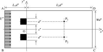
We consider the flow past a pair of square cylinders with width (and height)
 $d^{\ast }$
which are placed side by side with gap distance
 $s^{\ast }$
in a nominally uniform flow of velocity
 $U^{\ast }$
as illustrated in figure 1. The gap ratio
 ${\it\Gamma}$
is defined by
 ${\it\Gamma}=s^{\ast }/d^{\ast }$
, which plays an important role in the present problem. We take
 $x^{\ast }$
- and
 $y^{\ast }$
-axes along the streamwise direction and perpendicular to it, respectively, with the origin
 $\text{O}$
at the middle of the gap between the back faces of the cylinders. The two points indicated by
 $\text{P}_{1}$
(
 $(x_{1}^{\ast },y_{1}^{\ast })=(20d^{\ast },s^{\ast }/2+d^{\ast }/2)$
) and
 $\text{P}_{2}$
(
 $(x_{2}^{\ast },y_{2}^{\ast })=(20d^{\ast },-(s^{\ast }/2+d^{\ast }/2))$
) in figure 1 are chosen to observe oscillation in the flow. We note that figure 1 is not to scale, but neighbourhood of the two square cylinders is enlarged.
Configuration, the coordinates and the numerical domain. Two points
 $\text{P}_{1}$
and
 $\text{P}_{2}$
are chosen to observe oscillation in the flow.

The governing equations for the fluid motion are the Navier–Stokes and the continuity equations for the velocity
 $\boldsymbol{u}^{\ast }$
and the pressure
 $p^{\ast }$
. Assuming an incompressible two-dimensional flow, we introduce the stream function
 ${\it\psi}^{\ast }(x^{\ast },y^{\ast },t^{\ast })$
and the vorticity
 ${\it\omega}^{\ast }(x^{\ast },y^{\ast },t^{\ast })$
. Then the velocity
 $\boldsymbol{u}^{\ast }=(u^{\ast },v^{\ast })$
and the vorticity
 ${\it\omega}^{\ast }$
are expressed as
 $$\begin{eqnarray}u^{\ast }=\partial {\it\psi}^{\ast }/\partial y^{\ast },\quad v^{\ast }=-\partial {\it\psi}^{\ast }/\partial x^{\ast },\quad {\it\omega}^{\ast }=-{\it\Delta}^{\ast }{\it\psi}^{\ast },\quad {\it\Delta}^{\ast }=\left(\frac{\partial ^{2}}{\partial x^{\ast 2}}+\frac{\partial ^{2}}{\partial y^{\ast 2}}\right).\end{eqnarray}$$
Taking the uniform velocity
 $U^{\ast }$
and the width
 $d^{\ast }$
of the two square cylinders as the representative velocity and length scales, we make all of the physical quantities non-dimensional as
 $x=x^{\ast }/d^{\ast }$
,
 $y=y^{\ast }/d^{\ast }$
,
 $t=t^{\ast }U^{\ast }/d^{\ast }$
,
 $u=u^{\ast }/U^{\ast }$
,
 $v=v^{\ast }/U^{\ast }$
,
 ${\it\psi}={\it\psi}^{\ast }/(U^{\ast }d^{\ast })$
and
 ${\it\omega}={\it\omega}^{\ast }d^{\ast }/U^{\ast }$
. Here the non-dimensional physical quantities are indicated by omitting the asterisk (
 $\text{}^{\ast }$
) attached to the corresponding dimensional variables. Then, the governing equations of the flow, i.e. the vorticity transport and Poisson equations for the vorticity and the stream function, are written in the non-dimensional form as
 $$\begin{eqnarray}\displaystyle & \displaystyle \frac{\partial {\it\omega}}{\partial t}=N({\it\psi},\ {\it\omega})+\frac{1}{\mathit{Re}}{\rm\Delta}{\it\omega}, & \displaystyle\end{eqnarray}$$
 $$\begin{eqnarray}\displaystyle & {\it\omega}=-{\rm\Delta}{\it\psi}, & \displaystyle\end{eqnarray}$$
 $$\begin{eqnarray}\displaystyle & \displaystyle N({\it\psi},\ {\it\omega})=\frac{\partial {\it\psi}}{\partial x}\frac{\partial {\it\omega}}{\partial y}-\frac{\partial {\it\psi}}{\partial y}\frac{\partial {\it\omega}}{\partial x}, & \displaystyle\end{eqnarray}$$
 $\mathit{Re}$
is defined as
 $\mathit{Re}\equiv U^{\ast }d^{\ast }/{\it\nu}^{\ast }$
, and
 ${\it\nu}^{\ast }$
is the kinematic viscosity of the fluid.
In all numerical calculations including numerical simulations, and linear and weakly nonlinear stability analyses, the assumed infinitely-extended flow field is approximated by the finite domain with width
 $W$
and length
 $L_{1}+L_{2}$
indicated by ABCD in figure 1. Uniform flow with velocity
 $U=1$
is assumed on the upstream boundary AB:
 $$\begin{eqnarray}{\it\psi}=y,\quad {\it\omega}=0\quad (\text{AB}),\end{eqnarray}$$
and the boundary conditions on the side boundaries AD and BC are represented as
 $$\begin{eqnarray}\frac{\partial {\it\psi}}{\partial y}=1,\quad {\it\omega}=0\quad (\text{AD},\text{BC}).\end{eqnarray}$$
The outlet condition at the downstream boundary (CD) is approximated by the Sommerfeld radiation condition
 $$\begin{eqnarray}\frac{\partial {\it\psi}}{\partial t}+c\frac{\partial {\it\psi}}{\partial x}=0,\quad \frac{\partial {\it\omega}}{\partial t}+c\frac{\partial {\it\omega}}{\partial x}=0\quad (\text{CD}),\end{eqnarray}$$
where
 $c$
is the phase velocity of waves traveling through CD and is taken to be the local velocity in the
 $x$
direction at each point on CD. The non-slip boundary condition is applied on the cylinder surfaces, which is written as
 $$\begin{eqnarray}u=\frac{\partial {\it\psi}}{\partial y}=0,\quad v=-\frac{\partial {\it\psi}}{\partial x}=0.\end{eqnarray}$$
Since boundary conditions (2.8) are given for spatial derivatives of
 ${\it\psi}$
, the values of
 ${\it\psi}$
on the cylinder surfaces, say
 ${\it\psi}_{\text{B}1}$
and
 ${\it\psi}_{\text{B}2}$
, are unknown. In order to determine the values, we utilize the condition that the pressure
 $p$
has a single value at each point in the flow field, which is expressed as
 $$\begin{eqnarray}\oint _{C_{i}}\frac{\partial p}{\partial s}\text{d}s=0\end{eqnarray}$$
where
 $C_{i}$
(
 $i=1$
or 2) is taken along each cylinder surface. Equation (2.9) is written in terms of
 ${\it\psi}$
as
 $$\begin{eqnarray}\oint _{C_{i}}\frac{\partial ^{3}{\it\psi}}{\partial n^{3}}\text{d}s=0\end{eqnarray}$$
where
 $n$
and
 $s$
are the normal and parallel coordinates to the cylinder surface, respectively. Expressing (2.10) with
 ${\it\psi}_{\text{B}1}$
,
 ${\it\psi}_{\text{B}2}$
and
 ${\it\psi}$
at the points on the two nearest mesh lines to each cylinder surface, we solve Poisson equation (2.3) together with (2.10) to obtain
 ${\it\psi}_{\text{B}1}$
,
 ${\it\psi}_{\text{B}2}$
and the solution
 ${\it\psi}$
in the interior of the numerical domain.
2.1. Steady-state solution
At small Reynolds numbers, the flow is steady and symmetric with respect to the
 $x$
-axis, though it becomes unstable at larger Reynolds numbers than a critical value. The solution corresponding to the steady symmetric flow, say
 $(\overline{{\it\psi}},\overline{{\it\omega}})$
, satisfies basic (2.2) and (2.3) under boundary conditions (2.5)–(2.8) even for larger Reynolds numbers above the critical value, which we call the main flow and investigate its linear and weakly nonlinear stability to elucidate the nonlinear interaction between the two wakes. The stream function and the vorticity
 $(\overline{{\it\psi}},\overline{{\it\omega}})$
are odd functions of
 $y$
, i.e.
 $\overline{{\it\psi}}(x,-y)=-\overline{{\it\psi}}(x,y)$
and
 $\overline{{\it\omega}}(x,-y)=-\overline{{\it\omega}}(x,y)$
, and they are obtained numerically by solving the steady-state vorticity transport equation:
 $$\begin{eqnarray}N(\overline{{\it\psi}},\ \overline{{\it\omega}})+\frac{1}{\mathit{Re}}{\rm\Delta}\overline{{\it\omega}}=0\end{eqnarray}$$
together with the Poisson equation:
 $$\begin{eqnarray}\overline{{\it\omega}}=-{\rm\Delta}\overline{{\it\psi}},\end{eqnarray}$$
under the same boundary conditions for
 $({\it\psi},{\it\omega})$
including (2.5)–(2.8) and (2.10).
2.2. Linear and weakly nonlinear stability analyses
In order to investigate the stability of the steady symmetric flow, we consider a disturbance
 $(\widehat{{\it\psi}},\widehat{{\it\omega}})$
added to the main flow
 $(\overline{{\it\psi}},\overline{{\it\omega}})$
and express the vorticity and the stream function as
 $$\begin{eqnarray}{\it\psi}=\overline{{\it\psi}}+\widehat{{\it\psi}},\quad {\it\omega}=\overline{{\it\omega}}+\widehat{{\it\omega}},\end{eqnarray}$$
respectively. Substituting these expressions into (2.2) and subtracting (2.11) from the resultant equation, we obtain the disturbance equation as
 $$\begin{eqnarray}\frac{\partial \widehat{{\it\omega}}}{\partial t}=N(\widehat{{\it\psi}},\ \overline{{\it\omega}})+N(\overline{{\it\psi}},\ \widehat{{\it\omega}})+\frac{1}{\mathit{Re}}{\rm\Delta}\widehat{{\it\omega}}+N(\widehat{{\it\psi}},\ \widehat{{\it\omega}}).\end{eqnarray}$$
Similarly, the Poisson equation for
 $\widehat{{\it\psi}}$
is obtained as
 $$\begin{eqnarray}\widehat{{\it\omega}}=-{\rm\Delta}\widehat{{\it\psi}}.\end{eqnarray}$$
The boundary conditions for
 $(\widehat{{\it\psi}},\widehat{{\it\omega}})$
on the upstream and side boundaries are given as
 $$\begin{eqnarray}\widehat{{\it\psi}}=0,\quad \widehat{{\it\omega}}=0,\quad (\text{AD},\text{AB},\text{BC}).\end{eqnarray}$$
The outlet condition on the downstream boundary (CD) is taken as the Sommerfeld radiation condition
 $$\begin{eqnarray}\frac{\partial \widehat{{\it\psi}}}{\partial t}+c\frac{\partial \widehat{{\it\psi}}}{\partial x}=0,\quad \frac{\partial \widehat{{\it\omega}}}{\partial t}+c\frac{\partial \widehat{{\it\omega}}}{\partial x}=0\quad (\text{CD}),\end{eqnarray}$$
where
 $c$
is taken to be
 $\partial \overline{{\it\psi}}/\partial y$
at each point on CD. The non-slip boundary condition is taken on the surfaces of the square cylinders, which is written as
 $$\begin{eqnarray}\frac{\partial \widehat{{\it\psi}}}{\partial y}=0,\quad \frac{\partial \widehat{{\it\psi}}}{\partial x}=0.\end{eqnarray}$$
On the cylinder surfaces, the values of
 $\widehat{{\it\psi}}\ (=\widehat{{\it\psi}}_{\text{B}1},\ \widehat{{\it\psi}}_{\text{B}2})$
are determined in the same way as in the numerical simulations.
In the linear stability analysis, we neglect the nonlinear term of the disturbance
 $(\widehat{{\it\psi}},\widehat{{\it\omega}})$
in (2.14), and assume the time dependence of the disturbance as
 $\widehat{{\it\psi}}=\widetilde{{\it\psi}}(x,y)\text{e}^{{\it\lambda}t}$
and
 $\widehat{{\it\omega}}=\widetilde{{\it\omega}}(x,y)\text{e}^{{\it\lambda}t}$
. Then we obtain a linearized disturbance equation as
 $$\begin{eqnarray}{\it\lambda}\widetilde{{\it\omega}}=N(\widetilde{{\it\psi}},\ \overline{{\it\omega}})+N(\overline{{\it\psi}},\ \widetilde{{\it\omega}})+\frac{1}{\mathit{Re}}{\rm\Delta}\widetilde{{\it\omega}},\end{eqnarray}$$
which constitutes the eigenvalue problem for the linear stability analysis together with the Poisson equation
 $$\begin{eqnarray}\widetilde{{\it\omega}}=-{\rm\Delta}\widetilde{{\it\psi}},\end{eqnarray}$$
under the appropriate boundary conditions. The boundary conditions for
 $(\widetilde{{\it\psi}},\widetilde{{\it\omega}})$
are the same as for
 $(\widehat{{\it\psi}},\widehat{{\it\omega}})$
except that the condition
 $$\begin{eqnarray}{\it\lambda}\widetilde{{\it\psi}}+c\frac{\partial \widetilde{{\it\psi}}}{\partial x}=0,\quad {\it\lambda}\widetilde{{\it\omega}}+c\frac{\partial \widetilde{{\it\omega}}}{\partial x}=0,\end{eqnarray}$$
is used instead of (2.17). The solution of the eigenvalue problem gives an infinite number of eigenvalues,
 ${\it\lambda}$
and eigenfunctions (
 $\widetilde{{\it\psi}},\widetilde{{\it\omega}}$
), which are classified into symmetric and antisymmetric modes,
 $(\widetilde{{\it\psi}}_{s},\widetilde{{\it\omega}}_{s})$
and
 $(\widetilde{{\it\psi}}_{a},\widetilde{{\it\omega}}_{a})$
, according to the symmetry of the corresponding flow field with respect to the
 $x$
-axis. The eigenfunctions for the symmetric and antisymmetric modes are odd and even functions, respectively, so that the relations
 $\widetilde{{\it\psi}}_{s}(x,-y)=-\widetilde{{\it\psi}}_{s}(x,y)$
,
 $\widetilde{{\it\omega}}_{s}(x,-y)=-\widetilde{{\it\omega}}_{s}(x,y)$
and (
 $\widetilde{{\it\psi}}_{a}(x,-y)=\widetilde{{\it\psi}}_{a}(x,y)$
 $\widetilde{{\it\omega}}_{a}(x,-y)=\widetilde{{\it\omega}}_{a}(x,y)$
) hold. The eigenvalues,
 ${\it\lambda}$
(
 $={\it\sigma}-\text{i}{\it\mu}$
), are complex in general whose real and imaginary parts,
 ${\it\sigma}$
and
 ${\it\mu}$
, show the growth rate and the frequency (angular frequency) of the disturbance, respectively. Among infinite number of eigenmodes, the mode having the largest growth rate for each Reynolds number and gap ratio is called the most unstable mode. The Reynolds numbers at which the growth rate
 ${\it\sigma}$
of each mode vanishes are called neutral Reynolds numbers, above which the mode of disturbance grows, otherwise it decays, and the smallest neutral Reynolds number gives the critical state so that it is called a critical Reynolds number. As will be shown later, the antisymmetric mode determines the critical Reynolds number for smaller gap ratios than a threshold value, and the symmetric mode for larger gap ratios. There are two kinds of instability, one of which is the case of
 ${\it\mu}=0$
at the criticality where
 ${\it\sigma}$
vanishes, and in the other case
 ${\it\mu}\neq 0$
as in the present flow. In the former case, the growing disturbance is stationary and as a result of growth of stationary disturbance, another steady flow emerges from the main flow
 $(\overline{{\it\psi}},\overline{{\it\omega}})$
, i.e. the number of steady solution changes, which is called a pitchfork bifurcation when
 $(\overline{{\it\psi}},\overline{{\it\omega}})$
has a symmetry and the symmetry is broken due to the bifurcation. While in the latter case, the growing disturbance is oscillatory and the resultant flow due to the instability is oscillatory flow with the superposition of the oscillatory disturbance on the main flow. The emergence of oscillatory flow from the main flow is called a Hopf bifurcation in dynamical systems theory (see Drazin Reference Drazin1992, §1.6).
In the case where the symmetric steady flow is unstable only to one of the symmetric or antisymmetric modes of disturbance, the disturbance is expected to tend to an equilibrium state via nonlinearity of itself. On the other hand, if both modes are growing, they make nonlinear interactions with each other as well as with their own to lead to an equilibrium state. There are three possibilities for the equilibrium state, in which only one of the two modes survives overwhelming the other, or both modes have finite amplitudes. In considering the symmetries of the solution resulting from the nonlinear interactions, it is helpful to recall that
 ${\it\psi}(x,y,t)$
has the same symmetry both in
 $x$
and
 $y$
with
 ${\it\omega}(x,y,t)$
because the operator
 ${\it\Delta}$
does not change these symmetries. However, the nonlinear term
 $N({\it\psi},\ {\it\omega})$
in (2.2) yields a component of an odd function of
 $y$
if both
 ${\it\psi}(x,y,t)$
and
 ${\it\omega}(x,y,t)$
are even functions of
 $y$
, whereas it keeps the parity of function if both of them are odd. Note that, although it is confusing enough, the functions
 $\widetilde{{\it\psi}}_{s}$
and
 $\widetilde{{\it\omega}}_{s}$
for the symmetric mode are odd functions of
 $y$
, and their flow fields are symmetric with respect to the
 $x$
-axis. Since the symmetric mode of disturbance
 $\widetilde{{\it\psi}}_{s}$
is an odd function of
 $y$
so that
 $\widetilde{{\it\psi}}_{s}$
induces only symmetric higher harmonics in nonlinear states after interacting with the steady symmetric flow as well as with itself. However, as the antisymmetric mode is an even function of
 $y$
, it induces symmetric component as the first harmonic mode through nonlinear interaction of itself. Hence, in the case where only the symmetric mode survives the resultant equilibrium state displays a symmetric flow pattern, being superposed on the steady symmetric flow. On the other hand, even if only the antisymmetric mode survives the flow field is not antisymmetric, but asymmetric with respect to the
 $x$
-axis because it is a superposition of the antisymmetric disturbance on the steady symmetric flow. This flow property makes it difficult to evaluate the amplitude of the antisymmetric mode of disturbance in the nonlinear state from numerical simulation data. In order to resolve this difficulty, we need to appropriately define the amplitudes of the two modes.
We use Watson’s amplitude expansion method to derive the dynamical equations for the amplitudes of the two modes of disturbance,
 $A_{s}$
and
 $A_{a}$
, together with Herbert’s method to define the amplitudes of disturbance uniquely, taking consideration into the symmetry of the first harmonic component. We choose two points
 $\text{P}_{1}$
(
 $(x,y)=(20,({\it\Gamma}+1)/2)$
) and
 $\text{P}_{2}\ ((x,y)=(20,-({\it\Gamma}+1)/2))$
shown in figure 1 in defining the real-valued amplitudes of the antisymmetric and symmetric components of disturbance as
 $A_{s}=-(\partial \widehat{{\it\psi}}_{s}/\partial x)(\text{P}_{1})$
and
 $A_{a}=-(\partial \widehat{{\it\psi}}_{a}/\partial x)(\text{P}_{1})$
, following Herbert (Reference Herbert1983). With these definitions, the
 $y$
-components of velocity
 $v_{1}$
and
 $v_{2}$
at
 $\text{P}_{1}$
and
 $\text{P}_{2}$
are expressed as
 $v_{1}\!=-(\partial \widehat{{\it\psi}}_{s}/\partial x)(\text{P}_{1})\!-(\partial \widehat{{\it\psi}}_{a}/\partial x)(\text{P}_{1})$
and
 $v_{2}=(\partial \widehat{{\it\psi}}_{s}/\partial x)(\text{P}_{2})-(\partial \widehat{{\it\psi}}_{a}/\partial x)(\text{P}_{2})$
as long as we consider oscillation having only Fourier modes with the frequencies
 ${\it\mu}_{s}$
and
 ${\it\mu}_{a}$
.
We expand
 $\widehat{{\it\psi}}_{s}$
and
 $\widehat{{\it\psi}}_{a}$
in powers of
 $A_{s}$
and
 $A_{a}$
as well as in a Fourier series as
 $$\begin{eqnarray}\displaystyle \widehat{{\it\psi}}(x,y,t) & = & \displaystyle \mathop{\sum }\limits_{n=-\infty }^{\infty }A_{s}^{|n-1|+1}(t)\mathop{\sum }\limits_{m,\ell =0}^{\infty }A_{s}^{2m}(t)A_{a}^{2\ell }(t){\it\phi}_{snm\ell }(x,y)\text{e}^{-\text{i}n{\it\mu}_{s}t}\nonumber\\ \displaystyle & & \displaystyle +\,\mathop{\sum }\limits_{n=-\infty }^{\infty }A_{a}^{|n-1|+1}(t)\mathop{\sum }\limits_{m,\ell =0}^{\infty }A_{a}^{2m}(t)A_{s}^{2\ell }(t){\it\phi}_{anm\ell }(x,y)\text{e}^{-\text{i}n{\it\mu}_{a}t}.\end{eqnarray}$$
The expansion coefficient functions satisfy the relations
 $$\begin{eqnarray}{\it\phi}_{s(-n)m\ell }={\it\phi}_{snm\ell }^{\ast },\quad {\it\phi}_{a(-n)m\ell }={\it\phi}_{anm\ell }^{\ast }\end{eqnarray}$$
because of the reality of
 $\widehat{{\it\psi}}$
, where the asterisk denotes the complex conjugate hereafter. We also expand nonlinear growth rates
 ${\it\lambda}_{s}$
and
 ${\it\lambda}_{a}$
in powers of
 $A_{s}$
and
 $A_{a}$
, which gives
 $$\begin{eqnarray}{\it\lambda}_{s}=\mathop{\sum }\limits_{m,\ell =0}^{\infty }A_{s}^{2m}A_{a}^{2\ell }{\it\lambda}_{sm\ell },\quad {\it\lambda}_{a}=\mathop{\sum }\limits_{m,\ell =0}^{\infty }A_{a}^{2m}A_{s}^{2\ell }{\it\lambda}_{am\ell }.\end{eqnarray}$$
As the complex growth rates are denoted as
 ${\it\lambda}_{s}={\it\sigma}_{s}-\text{i}{\it\mu}_{s}$
and
 ${\it\lambda}_{a}={\it\sigma}_{a}-\text{i}{\it\mu}_{a}$
, equations (2.24) are equivalent to the expansions,
 $$\begin{eqnarray}{\it\sigma}_{s}-\text{i}{\it\mu}_{s}=\mathop{\sum }\limits_{m,\ell =0}^{\infty }A_{s}^{2m}A_{a}^{2\ell }({\it\sigma}_{sm\ell }-\text{i}{\it\mu}_{sm\ell }),\quad {\it\sigma}_{a}-\text{i}{\it\mu}_{a}=\mathop{\sum }\limits_{m,\ell =0}^{\infty }A_{a}^{2m}A_{s}^{2\ell }({\it\sigma}_{am\ell }-\text{i}{\it\mu}_{am\ell }).\end{eqnarray}$$
Note that the real parts of the complex growth rates,
 ${\it\sigma}_{s}$
and
 ${\it\sigma}_{a}$
, are expressed in terms of
 $A_{s}$
and
 $A_{a}$
as
 $$\begin{eqnarray}{\it\sigma}_{s}=\frac{1}{A_{s}}\frac{\text{d}A_{s}}{\text{d}t},\quad {\it\sigma}_{a}=\frac{1}{A_{a}}\frac{\text{d}A_{a}}{\text{d}t},\end{eqnarray}$$
respectively.
The basic equations governing the time development of the disturbance,
 $\widehat{{\it\psi}}$
and
 $\widehat{{\it\omega}}$
, are (2.14) and (2.15), which we express symbolically in a simple form by using only
 $\widehat{{\it\psi}}$
as
 $$\begin{eqnarray}\frac{\partial {\rm\Delta}\widehat{{\it\psi}}}{\partial t}=\mathscr{L}\widehat{{\it\psi}}+\mathscr{N}(\widehat{{\it\psi}},\widehat{{\it\psi}}),\end{eqnarray}$$
where
 $\mathscr{L}\widehat{{\it\psi}}$
and
 $\mathscr{N}(\widehat{{\it\psi}}_{1},\widehat{{\it\psi}}_{2})$
are defined as
 $$\begin{eqnarray}\mathscr{L}\widehat{{\it\psi}}=\mathscr{N}(\overline{{\it\psi}},\widehat{{\it\psi}})+\mathscr{N}(\widehat{{\it\psi}},\overline{{\it\psi}})+\frac{1}{\mathit{Re}}{\rm\Delta}{\rm\Delta}\widehat{{\it\psi}},\quad \mathscr{N}(\widehat{{\it\psi}}_{1},\widehat{{\it\psi}}_{2})=\frac{\partial \widehat{{\it\psi}}_{1}}{\partial x}\frac{\partial {\rm\Delta}\widehat{{\it\psi}}_{2}}{\partial y}-\frac{\partial \widehat{{\it\psi}}_{1}}{\partial y}\frac{\partial {\rm\Delta}\widehat{{\it\psi}}_{2}}{\partial x}.\end{eqnarray}$$
Substituting (2.22), (2.24) and (2.26) into (2.27), and equating the same Fourier component and the same power of the amplitude like
 $A_{s}^{2m+n}A_{a}^{2\ell }\text{e}^{-\text{i}n{\it\mu}_{s}t}$
or
 $A_{a}^{2m+n}A_{s}^{2\ell }\text{e}^{-\text{i}n{\it\mu}_{a}t}$
, we obtain a set of equations for the expansion coefficient functions
 ${\it\phi}_{snm\ell }$
and
 ${\it\phi}_{anm\ell }$
. Among the resultant infinite sets of equations, the lowest-order equations of
 $O(A_{s})$
or
 $O(A_{a})$
are nothing but the linear stability (2.19) and (2.20), which are expressed simply as
 $$\begin{eqnarray}({\it\lambda}_{s00}{\it\Delta}-\mathscr{L}){\it\phi}_{s100}=0,\quad ({\it\lambda}_{a00}{\it\Delta}-\mathscr{L}){\it\phi}_{a100}=0.\end{eqnarray}$$
Since (2.29) for
 ${\it\phi}_{s100}$
and
 ${\it\phi}_{a100}$
are linear and homogeneous, and their boundary conditions are as well, we normalize them to be
 $-(\partial {\it\phi}_{s100}/\partial x)(\text{P}_{1})=1$
and
 $-(\partial {\it\phi}_{a100}/\partial x)(\text{P}_{1})=1$
, being consistent with the definitions of
 $A_{s}$
and
 $A_{a}$
.
At the second order of
 $O(A_{s}^{2})$
or
 $O(A_{a}^{2})$
, we obtain the equations for the mean flow distortions (
 ${\it\phi}_{s010}$
,
 ${\it\phi}_{a010}$
) and the first harmonic modes (
 ${\it\phi}_{s200}$
,
 ${\it\phi}_{a200}$
) as
 $$\begin{eqnarray}\left.\begin{array}{@{}l@{}}(2{\it\sigma}_{s00}{\it\Delta}-\mathscr{L}){\it\phi}_{s010}=\mathscr{N}({\it\phi}_{s100}^{\ast },{\it\phi}_{s100})+\mathscr{N}({\it\phi}_{s100},{\it\phi}_{s100}^{\ast }),\\ (2{\it\sigma}_{a00}{\it\Delta}-\mathscr{L}){\it\phi}_{a010}=\mathscr{N}({\it\phi}_{a100}^{\ast },{\it\phi}_{a100})+\mathscr{N}({\it\phi}_{a100},{\it\phi}_{a100}^{\ast }),\end{array}\right\}\end{eqnarray}$$
and
 $$\begin{eqnarray}(2{\it\lambda}_{s00}{\it\Delta}-\mathscr{L}){\it\phi}_{s200}=\mathscr{N}({\it\phi}_{s100},{\it\phi}_{s100}),\quad (2{\it\lambda}_{a00}{\it\Delta}-\mathscr{L}){\it\phi}_{a200}=\mathscr{N}({\it\phi}_{a100},{\it\phi}_{a100}),\end{eqnarray}$$
respectively. As (2.30) and (2.31) are also linear, but inhomogeneous, we can solve these equations under the homogeneous boundary conditions similar to (2.16)–(2.18).
At the third order of
 $O(A_{s}^{3})$
,
 $O(A_{a}^{3})$
,
 $O(A_{s}A_{a}^{2})$
or
 $O(A_{s}^{2}A_{a})$
, we obtain the equations for
 ${\it\phi}_{s110}$
,
 ${\it\phi}_{a110}$
,
 ${\it\phi}_{s101}$
and
 ${\it\phi}_{a101}$
as
 $$\begin{eqnarray}\left.\begin{array}{@{}l@{}}\left[(2{\it\sigma}_{s00}+{\it\lambda}_{s00}){\it\Delta}-\mathscr{L}\right]{\it\phi}_{s110}=-{\it\lambda}_{s10}{\rm\Delta}{\it\phi}_{s100}+\mathscr{N}({\it\phi}_{s010},{\it\phi}_{s100})+\mathscr{N}({\it\phi}_{s100},{\it\phi}_{s010})\\ \qquad \qquad \qquad \qquad \qquad \qquad \quad +\,\mathscr{N}({\it\phi}_{s100}^{\ast },{\it\phi}_{s200})+\mathscr{N}({\it\phi}_{s200},{\it\phi}_{s100}^{\ast }),\\ \left[(2{\it\sigma}_{a00}+{\it\lambda}_{a00}){\it\Delta}-\mathscr{L}\right]{\it\phi}_{a110}=-{\it\lambda}_{a10}{\rm\Delta}{\it\phi}_{a100}+\mathscr{N}({\it\phi}_{a010},{\it\phi}_{a100})+\mathscr{N}({\it\phi}_{a100},{\it\phi}_{a010})\\ \qquad \qquad \qquad \qquad \qquad \qquad \quad +\,\mathscr{N}({\it\phi}_{a100}^{\ast },{\it\phi}_{a200})+\mathscr{N}({\it\phi}_{a200},{\it\phi}_{a100}^{\ast }).\\ \left[(2{\it\sigma}_{a00}+{\it\lambda}_{s00}){\it\Delta}-\mathscr{L}\right]{\it\phi}_{s101}=-{\it\lambda}_{s01}{\rm\Delta}{\it\phi}_{s100}+\mathscr{N}({\it\phi}_{s100},\ {\it\phi}_{a010})+\mathscr{N}({\it\phi}_{a010},{\it\phi}_{s100}),\\ \left[(2{\it\sigma}_{s00}+{\it\lambda}_{a00}){\it\Delta}-\mathscr{L}\right]{\it\phi}_{a101}=-{\it\lambda}_{a01}{\rm\Delta}{\it\phi}_{a100}+\mathscr{N}({\it\phi}_{a100},{\it\phi}_{s010})+\mathscr{N}\ ({\it\phi}_{s010},\ {\it\phi}_{a100}).\end{array}\right\}\end{eqnarray}$$
Equations (2.32) for
 ${\it\phi}_{s110}$
,
 ${\it\phi}_{a110}$
,
 ${\it\phi}_{s101}$
and
 ${\it\phi}_{a101}$
include unknown constants
 ${\it\lambda}_{s10}$
,
 ${\it\lambda}_{a10}$
,
 ${\it\lambda}_{s01}$
and
 ${\it\lambda}_{a01}$
, so that we need some technique in solving these equations. We will follow Watson (Reference Watson1960) to solve the equations and express the solutions as
 $$\begin{eqnarray}\left.\begin{array}{@{}l@{}}{\it\phi}_{s110}={\it\lambda}_{s10}{\it\chi}_{s010}+{\it\chi}_{s110},\quad {\it\phi}_{a110}={\it\lambda}_{a10}{\it\chi}_{a010}+{\it\chi}_{a110},\\ {\it\phi}_{s101}={\it\lambda}_{s01}{\it\chi}_{s001}+{\it\chi}_{s101},\quad {\it\phi}_{a101}={\it\lambda}_{a01}{\it\chi}_{a001}+{\it\chi}_{a101}.\end{array}\right\}\end{eqnarray}$$
Substituting (2.33) into (2.32) and equating the terms including the factors
 ${\it\lambda}_{s10}$
,
 ${\it\lambda}_{a10}$
,
 ${\it\lambda}_{s01}$
and
 ${\it\lambda}_{a01}$
, we obtain the equations for
 ${\it\chi}_{s010}$
,
 ${\it\chi}_{a010}$
,
 ${\it\chi}_{s001}$
and
 ${\it\chi}_{a001}$
, which are easily solved as
 $$\begin{eqnarray}{\it\chi}_{s010}=-{\it\phi}_{s100}/(2{\it\sigma}_{s00}),\quad {\it\chi}_{a010}=-{\it\phi}_{a100}/(2{\it\sigma}_{a00}),\end{eqnarray}$$
 $$\begin{eqnarray}{\it\chi}_{s001}=-{\it\phi}_{s100}/(2{\it\sigma}_{a00}),\quad {\it\chi}_{a001}=-{\it\phi}_{a100}/(2{\it\sigma}_{s00}).\end{eqnarray}$$
On the other hand, the equations for
 ${\it\chi}_{s110}$
,
 ${\it\chi}_{a110}$
,
 ${\it\chi}_{s101}$
and
 ${\it\chi}_{a101}$
consist of terms which are left in (2.32) after subtracting the terms including the factors
 ${\it\lambda}_{s10}$
,
 ${\it\lambda}_{a10}$
,
 ${\it\lambda}_{s01}$
and
 ${\it\lambda}_{a01}$
, and are expressed as
 $$\begin{eqnarray}\left.\begin{array}{@{}l@{}}\left[(2{\it\sigma}_{s00}+{\it\lambda}_{s00}){\it\Delta}-\mathscr{L}\right]{\it\chi}_{s110}=\mathscr{N}({\it\phi}_{s010},\ {\it\phi}_{s100})+\mathscr{N}({\it\phi}_{s100},\ {\it\phi}_{s010})\\ \qquad \qquad \qquad \qquad \qquad \qquad \quad +\,\mathscr{N}({\it\phi}_{s100}^{\ast },\ {\it\phi}_{s200})+\mathscr{N}({\it\phi}_{s200},\ {\it\phi}_{s100}^{\ast }),\\ \left[(2{\it\sigma}_{a00}+{\it\lambda}_{a00}){\it\Delta}-\mathscr{L}\right]{\it\chi}_{a110}=\mathscr{N}({\it\phi}_{a010},\ {\it\phi}_{a100})+\mathscr{N}({\it\phi}_{a100},\ {\it\phi}_{a010})\\ \qquad \qquad \qquad \qquad \qquad \qquad \quad +\,\mathscr{N}({\it\phi}_{a100}^{\ast },\ {\it\phi}_{a200})+\mathscr{N}({\it\phi}_{a200},\ {\it\phi}_{a100}^{\ast }),\\ \left[(2{\it\sigma}_{a00}+{\it\lambda}_{s00}){\it\Delta}-\mathscr{L}\right]{\it\chi}_{s101}=\mathscr{N}({\it\phi}_{s100},\ {\it\phi}_{a010})+\mathscr{N}({\it\phi}_{a010},\ {\it\phi}_{s100}),\\ \left[(2{\it\sigma}_{s00}+{\it\lambda}_{a00}){\it\Delta}-\mathscr{L}\right]{\it\chi}_{a101}=\mathscr{N}({\it\phi}_{a100},\ {\it\phi}_{s010})+\mathscr{N}({\it\phi}_{s010},\ {\it\phi}_{a100}).\end{array}\right\}\end{eqnarray}$$
The functions
 ${\it\chi}_{s1m\ell }$
and
 ${\it\chi}_{a1m\ell }$
with
 $\ell +m>0$
are obtained without any arbitrary constants by solving inhomogeneous equations (2.36) under the boundary conditions similar to (2.16)–(2.18).
The expansion coefficients
 ${\it\lambda}_{s10}$
,
 ${\it\lambda}_{a10}$
,
 ${\it\lambda}_{s01}$
and
 ${\it\lambda}_{a01}$
of
 ${\it\lambda}_{s}$
and
 ${\it\lambda}_{a}$
in (2.24) are expressed in terms of
 ${\it\chi}_{s1m\ell }$
and
 ${\it\chi}_{a1m\ell }\ (\ell +m>0)$
as
 $$\begin{eqnarray}\left.\begin{array}{@{}l@{}}\displaystyle {\it\lambda}_{s10}=-2{\it\sigma}_{s00}\frac{\partial {\it\chi}_{s110}}{\partial x}(\text{P}_{1}),\quad {\it\lambda}_{a10}=-2{\it\sigma}_{a00}\frac{\partial {\it\chi}_{a110}}{\partial x}(\text{P}_{1}),\vspace{3.0pt}\\ \displaystyle {\it\lambda}_{s01}=-2{\it\sigma}_{a00}\frac{\partial {\it\chi}_{s101}}{\partial x}(\text{P}_{1}),\quad {\it\lambda}_{a01}=-2{\it\sigma}_{s00}\frac{\partial {\it\chi}_{a101}}{\partial x}(\text{P}_{1}),\end{array}\right\}\end{eqnarray}$$
where we used the relations
 $(\partial {\it\phi}_{s1m\ell }/\partial x)(\text{P}_{1})=0$
and
 $(\partial {\it\phi}_{a1m\ell }/\partial x)(\text{P}_{1})=0$
, for (
 $\ell +m>0$
) which come from the unique definitions of
 $A_{s}$
and
 $A_{a}$
at
 $\text{P}_{1}$
. Thus, we have determined all of the expansion coefficients in (2.24). Defining two complex amplitudes
 $\widetilde{A}_{s}$
and
 $\widetilde{A}_{a}$
by
 $\widetilde{A}_{s}=A_{s}\text{e}^{-\text{i}{\it\mu}_{s}t}$
and
 $\widetilde{A}_{a}=A_{a}\text{e}^{-\text{i}{\it\mu}_{a}t}$
, we finally obtain a set of amplitude equations for the complex amplitudes
 $\widetilde{A}_{s}$
and
 $\widetilde{A}_{a}$
as
 $$\begin{eqnarray}\left.\begin{array}{@{}l@{}}\displaystyle \frac{\text{d}\widetilde{A}_{s}}{\text{d}t}={\it\lambda}_{s00}\widetilde{A}_{s}+{\it\lambda}_{s10}|\widetilde{A}_{s}|^{2}\widetilde{A}_{s}+{\it\lambda}_{s01}|\widetilde{A}_{a}|^{2}\widetilde{A}_{s},\\ \displaystyle \frac{\text{d}\widetilde{A}_{a}}{\text{d}t}={\it\lambda}_{a00}\widetilde{A}_{a}+{\it\lambda}_{a10}|\widetilde{A}_{a}|^{2}\widetilde{A}_{a}+{\it\lambda}_{a01}|\widetilde{A}_{s}|^{2}\widetilde{A}_{a}.\end{array}\right\}\end{eqnarray}$$
3. Numerical methods
3.1. Numerical methods and accuracy assessments
In numerical simulations, numerical domain ABCD is discretized with a non-uniform rectangular mesh having variable differences
 ${\rm\Delta}x$
and
 ${\rm\Delta}y$
in the
 $x$
and
 $y$
directions. The mesh sizes
 ${\rm\Delta}x$
and
 ${\rm\Delta}y$
are smallest near the cylinder surface, and become larger going away from it, finally reaching constant values beyond prescribed distances. The spatial derivatives are approximated with the central finite difference of fourth-order accuracy. The vorticity transport equation (2.2) is solved under the appropriate boundary and initial conditions by approximating the time derivative with the fourth-order Runge–Kutta method taking a finite difference
 ${\rm\Delta}t$
. The Poisson equation (2.3) for
 ${\it\psi}$
is solved under the appropriate boundary conditions with the SOR (successive over-relaxation) method.
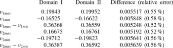
The extent of the numerical domain is crucial to assure the accuracy of numerical results. In order to study the effect of the extent of the numerical domain, we obtain maximum (
 $v_{1max}$
,
 $v_{2max}$
) and minimum (
 $v_{1min}$
,
 $v_{2min}$
) values and amplitudes (
 $v_{1max}-v_{1min}$
,
 $v_{2max}-v_{2min}$
) of oscillation in the velocities
 $v_{1}$
and
 $v_{2}$
at
 $\text{P}_{1}$
(
 $(x,y)=(20,{\it\Gamma}/2+1/2)$
) and
 $\text{P}_{2}$
(
 $(x,y)=(20,-{\it\Gamma}/2-1/2)$
). We compare these values between numerical domain I (
 $L_{1}=9.96$
,
 $L_{2}=140.1$
,
 $W=40$
) and domain II (
 $L_{1}=19.4$
,
 $L_{2}=280.2$
,
 $W=80$
) for
 $\mathit{Re}=60$
and
 ${\it\Gamma}=2.0$
in table 1. The relative errors are smaller than
 $0.6\,\%$
. Hence, we adopt numerical domain I in our numerical simulations.
Numerical domain assessment,
 $\mathit{Re}=60$
,
 ${\it\Gamma}=2.0$
. Domain I:
 $L_{1}=9.96$
,
 $L_{2}=140.1$
,
 $W=40$
. Domain II:
 $L_{1}=19.4$
,
 $L_{2}=280.2$
,
 $W=80$
.

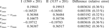
We carried out assessments of appropriateness of the number of mesh points, where we compare the values (
 $v_{1max}$
,
 $v_{2max}$
,
 $v_{1min}$
,
 $v_{2min}$
,
 $v_{1max}-v_{1min}$
,
 $v_{2max}-v_{2min}$
) by taking two different numbers of mesh points, i.e. I (
 $1569\times 201$
) and II (
 $3137\times 201$
). These values are tabulated in table 2. At
 $\mathit{Re}=60$
and
 ${\it\Gamma}=2.0$
, the relative errors between I and II are smaller than
 $0.4\,\%$
, so that we adopt I (
 $1569\times 201$
) as the number of mesh points in our numerical simulations, in which 20 mesh points are taken along each side of the square cylinders.
Assessment of the number of mesh points,
 $\mathit{Re}=60$
,
 ${\it\Gamma}=2.0$
.

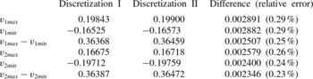
The magnitude of finite difference
 ${\rm\Delta}t$
in time discretization is also assessed by evaluating the oscillation amplitudes
 $v_{1max}-v_{1min}$
and
 $v_{2max}-v_{2min}$
for two finite differences
 ${\rm\Delta}t=0.001$
and 0.002. The relative errors between the two cases are smaller than
 $0.3\,\%$
for
 $\mathit{Re}=60$
and
 ${\it\Gamma}=2.0$
as shown in table 3, and we adopt
 ${\rm\Delta}t=0.002$
.
Assessment of the finite differences in the temporal discretization,
 ${\rm\Delta}t$
. Discretization I:
 ${\rm\Delta}t=0.002$
. Discretization II:
 ${\rm\Delta}t=0.001$
.

3.2. Linear and weakly nonlinear stability analyses
In numerical calculations of the steady symmetric flow and linear and weakly nonlinear stability analyses, we use the same non-uniform rectangular mesh adopted in numerical simulation, and approximate the spatial derivatives with the central finite difference of fourth-order accuracy. The eigenvalue problem composed of the linear disturbance equation (2.29) and the appropriate boundary conditions is solved with the double QR method. Inhomogeneous equations, (2.30), (2.31) and (2.36), are solved under the appropriate boundary conditions with the SOR iteration method, where convergence is determined when the maximum differences between two consecutive iteration values of
 ${\it\psi}$
and
 ${\it\omega}$
over the entire numerical domain becomes less than
 $1\times 10^{-7}$
.
4. Numerical results
4.1. Linear stability analysis of the steady symmetric flow
We have obtained the steady symmetric flow numerically by solving (2.11) and (2.12) under the boundary conditions (2.5)–(2.8) and (2.10), and analysed its linear stability by solving the eigenvalue problem consisting of (2.19), (2.20) and the boundary conditions for
 $\widetilde{{\it\psi}}$
and
 $\widetilde{{\it\omega}}$
for each Reynolds number and each gap ratio in the range of
 $1.0\leqslant {\it\Gamma}\leqslant 3.5$
. The complex linear growth ratio
 ${\it\lambda}\ (={\it\sigma}-\text{i}{\it\mu})$
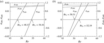
thus obtained is depicted in figure 2(a) for
 ${\it\Gamma}=2.0$
, for instance, where the solid and broken lines indicate the real part
 ${\it\sigma}$
and imaginary part
 ${\it\mu}$
, respectively. The antisymmetric mode of disturbance has a larger linear growth rate, say
 ${\it\sigma}_{a00}$
, than the symmetric mode (
 ${\it\sigma}_{s00}$
) throughout the range of Reynolds number depicted in this figure. The critical and neutral Reynolds numbers are evaluated as
 $\mathit{Re}_{a}=48.17$
and
 $\mathit{Re}_{s}=54.41$
for the antisymmetric and symmetric modes, respectively, and hence the flow becomes unstable to the antisymmetric mode first for
 ${\it\Gamma}=2.0$
. The angular velocities, say
 ${\it\mu}_{s00}$
and
 ${\it\mu}_{a00}$
, increase very slowly with
 $\mathit{Re}$
being almost constant, and the symmetric mode has a larger value of
 ${\it\mu}_{s00}$
than the antisymmetric mode (
 ${\it\mu}_{a00}$
). The Strouhal numbers
 $\mathit{St}$
are evaluated for both modes as
 $\mathit{St}_{s}={\it\mu}_{s00}/(2{\rm\pi})=0.1584$
,
 $\mathit{St}_{a}={\it\mu}_{a00}/(2{\rm\pi})=0.1418$
at the criticality, respectively. On the other hand, in the case of
 ${\it\Gamma}=2.5$
the symmetric mode gives the critical condition as seen in figure 2(b), having a larger linear growth rate
 ${\it\sigma}_{s00}$
than the antisymmetric mode (
 ${\it\sigma}_{a00}$
). The critical and neutral Reynolds numbers are
 $\mathit{Re}_{s}=50.31$
and
 $\mathit{Re}_{a}=52.19$
, and the Strouhal numbers are
 $\mathit{St}_{s}=0.1640$
,
 $\mathit{St}_{a}=0.1490$
at each critical state.
Linear growth rate
 ${\it\lambda}$
: (a)
 ${\it\Gamma}=2.0$
; (b)
 ${\it\Gamma}=2.5$
. Solid line: real part
 ${\it\sigma}$
. Broken line: imaginary part
 ${\it\mu}$
.

As no appropriate experimental or numerical data are found to compare with our linear stability results at similar Reynolds numbers, we compare them with numerical simulation data performed at rather larger Reynolds number of
 $\mathit{Re}=100$
by Kang (Reference Kang2003), where Strouhal numbers
 $\mathit{St}_{s}=0.177$
and
 $\mathit{St}_{a}=0.168$
are reported for circular cylinder case with
 ${\it\Gamma}=2.0$
. Our values of
 $\mathit{St}_{s}$
and
 $\mathit{St}_{a}$
are a little smaller than Kang’s numerical values, because of the smaller value of the Reynolds number at the criticality in the present analysis and the difference of the cylinder shape.
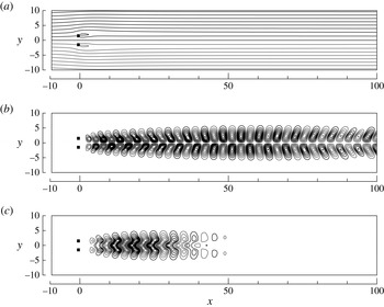
We show the steady symmetric flow and the flow fields of the eigenfunctions corresponding to the two most unstable modes in the linear stability analysis in figure 3 for
 ${\it\Gamma}=2.0$
and
 $\mathit{Re}=60$
as typical examples. The flow pattern of the steady symmetric flow is plain as shown in figure 3(a), which almost keeps its shape even for different Reynolds numbers, with only the length of the attached vortex being longer for larger Reynolds numbers. The real part of the eigenfunction
 $\widetilde{{\it\psi}}_{s}$
for the symmetric mode of disturbance is an odd function of
 $y$
. The flow field of
 $\widetilde{{\it\psi}}_{s}$
is depicted in figure 3(b) by contour lines, which consists of two lines of vortices, where the dark and light lines indicate contours of positive and negative values of
 $\widetilde{{\it\psi}}_{s}$
, respectively. Each couple of adjacent and facing vortices have opposite senses of rotation. This mode of disturbance yields a symmetric flow field characterized by double vortex streets. Note that the contour lines of
 $\widetilde{{\it\psi}}_{s}$
extend over the whole range of this figure up to
 $x=100$
, while the eigenfunction
 $\widetilde{{\it\psi}}_{a}$
for the antisymmetric mode diminishes in magnitude in a shorter distance than
 $x\sim 50$
as shown in figure 3(c). The rapid decay of the eigenfunctions is responsible to early annihilation of the two vortex streets antisymmetrically arranged behind the cylinders, and the asymmetric flow induced by the antisymmetric mode of disturbance loses its initial vortex configuration after advected only in a short distance behind the cylinders, as will be explained in § 5. The imaginary parts of the eigenfunctions are similar to the corresponding real parts except phase differences, so that they are omitted to be shown to save space.
Steady symmetric flow and the eigenfunctions corresponding to the two most unstable modes in the linear stability analysis (contour lines of stream function),
 $\mathit{Re}=60$
,
 ${\it\Gamma}=2.0$
: (a) steady symmetric flow (main flow); (b) symmetric mode of disturbance; (c) antisymmetric mode of disturbance.

The neutral Reynolds numbers, at which each of the growth rates
 ${\it\sigma}_{s00}$
and
 ${\it\sigma}_{s00}$
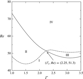
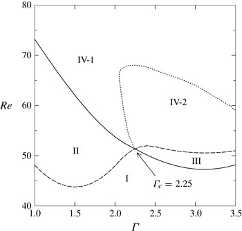
of symmetric and antisymmetric modes of disturbance vanishes, are shown in figure 4, where the solid and broken lines indicate the symmetric and antisymmetric modes, respectively. The two lines intersect at a point
 $({\it\Gamma}_{c},Re)=(2.25,51.3)$
. We call the gap ratio
 ${\it\Gamma}_{c}=2.25$
the threshold gap ratio. For smaller gap ratios than this value (
 ${\it\Gamma}<{\it\Gamma}_{c}$
), an antisymmetric mode of disturbance is the most unstable mode, while for
 ${\it\Gamma}>{\it\Gamma}_{c}$
the most unstable mode is a symmetric mode. The parameter domain of (
 ${\it\Gamma}$
,
 $\mathit{Re}$
) is classified by the symmetry of the growing mode(s) of disturbance into four regions I, II, III and IV as shown in figure 4. In region I, the steady symmetric flow is stable to both modes of disturbance (
 ${\it\sigma}_{s00}<0$
,
 ${\it\sigma}_{a00}<0$
). Regions II and III shows that the steady symmetric flow is unstable only to the antisymmetric (
 ${\it\sigma}_{a00}>0$
,
 ${\it\sigma}_{s00}<0$
) or the symmetric mode (
 ${\it\sigma}_{s00}>0$
,
 ${\it\sigma}_{a00}<0$
), respectively. Region IV (
 ${\it\sigma}_{s00}>0$
,
 ${\it\sigma}_{a00}>0$
) is the parameter region that we are now concerned with, in which both modes are growing. When the both modes grow, they compete with each other through nonlinear interactions between them. As a result of the competition, one of the symmetric and antisymmetric modes of disturbance survive overwhelming the other, or both modes remains having finite amplitudes. The resultant equilibrium state of the total flow is established as a superposition of the surviving mode(s) of disturbance on the steady symmetric flow.
Critical Reynolds number as a function of the gap ratio: solid line, symmetric mode; broken line, antisymmetric mode; I, steady symmetric flow; II, unstable to the antisymmetric mode of disturbance; III, unstable to the symmetric mode of disturbance; IV, unstable to the both antisymmetric and symmetric modes of disturbance.

It is noted here that the linear stability of the flow behind two circular cylinders shows similar behaviour to the present case of square cylinders, although differences between the flows around square and circular cylinders are often overemphasized. The critical gap ratio is
 ${\it\Gamma}_{c}=2.34$
at
 $\mathit{Re}_{c}=45.2$
for the circular cylinders, across which the most unstable mode changes from the antisymmetric to the symmetric mode similarly to the square cylinder case as shown by Akinaga & Mizushima (Reference Akinaga and Mizushima2005).
4.2. Weakly nonlinear stability analysis
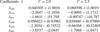
We have evaluated all of the coefficients included in the coupled amplitude equations (2.38) by numerically solving (2.30), (2.31) and (2.36) under the appropriate boundary conditions for parameter values in region IV. Among numerous sets of numerical results, we show only two cases of
 ${\it\Gamma}=2.0$
and 2.5 at the same Reynolds number
 $\mathit{Re}=60$
in table 4, as typical examples. The two gap ratios
 ${\it\Gamma}=2.0$
and 2.5 are chosen as representative cases where the antisymmetric or the symmetric mode of disturbance gives the critical condition, respectively. Needless to say, the real parts of
 ${\it\lambda}_{s00}$
and
 ${\it\lambda}_{a00}$
are positive in these tables because we are considering the cases where both modes are growing, only for which case the amplitude equations are applicable. It is noticeable that the real parts of
 ${\it\lambda}_{s10}$
,
 ${\it\lambda}_{s01}$
,
 ${\it\lambda}_{a10}$
and
 ${\it\lambda}_{a01}$
are all negative, which we assume for other values of
 ${\it\Gamma}$
in the following discussion on the existence and stability of the equilibrium solutions of the amplitude equations.
Coefficients of the coupled amplitude equations,
 $\mathit{Re}=60$
.

In order to explore nonlinear behaviors of the complex amplitudes we solved the coupled amplitude equations for (
 $\widetilde{A}_{s}(t)$
,
 $\widetilde{A}_{a}(t)$
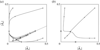
) as an initial value problem and plotted their traces in phase diagrams in figure 5 for the two cases
 ${\it\Gamma}=2.0$
and 2.5 at
 $\mathit{Re}=60$
. In these figures, the horizontal and vertical axes stand for the absolute values
 $|\widetilde{A}_{s}|$
and
 $|\widetilde{A}_{a}|$
of the amplitudes of the symmetric and the antisymmetric modes. The open circles indicate the initial state (
 $|\widetilde{A}_{s}(t=0)|$
,
 $|\widetilde{A}_{a}(t=0)|$
) which can be chosen arbitrarily. The time-dependent solution proceeds along each line in the direction of the arrow and finally approaches to the equilibrium state indicated by filled circles. In figure 5(a), the flow converges to one of the two single-mode solutions, (
 $|\widetilde{A}_{s}|\neq 0,|\widetilde{A}_{a}|=0$
) or (
 $|\widetilde{A}_{s}|=0,|\widetilde{A}_{a}|\neq 0$
), depending on the initial condition for
 ${\it\Gamma}=2.0$
, which tells us that the equilibrium state is not determined uniquely, but depends on the initial state. Although there is no orbit converging to a mixed-mode solution (
 $|\widetilde{A}_{s}|\neq 0,|\widetilde{A}_{a}|\neq 0$
) because it is unstable, we can evaluate the amplitudes of the mixed-mode solution from (2.38), which is indicated by the cross symbol in figure 5(a). In the case of
 ${\it\Gamma}=2.5$
(figure 5
b), the solution converges to the mixed-mode solution indicated by the filled circle and the single-mode solutions (crosses in figure 6
b) are unstable so could not be attained. Thus, the equilibrium solution is uniquely determined independently of the initial condition in this case.
Phase diagram of the solution obtained by the coupled Landau equations,
 $\mathit{Re}=60$
: solid line, orbit; ○, initial condition; ●, equilibrium amplitude;
 $\times$
, unsteady equilibrium solution; (a)
 ${\it\Gamma}=2.0$
; (b)
 ${\it\Gamma}=2.5$
.

As we are interested in the equilibrium flow resulting from nonlinear interactions between the two modes of disturbance, we evaluate the equilibrium amplitudes of the two modes and investigate their stability. The equilibrium solutions (
 $\overline{A}_{s}$
,
 $\overline{A}_{a}$
) of the coupled amplitude equations (2.38) are expressed as
 $\overline{A}_{s}=|\overline{A}_{s}|\exp (\text{i}{\it\mu}_{s}t)$
and
 $\overline{A}_{a}=|\overline{A}_{a}|\exp (\text{i}{\it\mu}_{a}t)$
with
 $\text{d}|\overline{A}_{s}|/\text{d}t=0$
and
 $\text{d}|\overline{A}_{a}|/\text{d}t=0$
. There are four possible equilibrium solutions, i.e. the null solution
 $(|\overline{A}_{s}|=0,\ |\overline{A}_{a}|=0)$
, a symmetric single-mode solution
 $(|\overline{A}_{s}|\neq 0,\ |\overline{A}_{a}|=0)$
, an antisymmetric single-mode solution
 $(|\overline{A}_{s}|=0,\ |\overline{A}_{a}|\neq 0)$
, and a mixed solution
 $(|\overline{A}_{s}|\neq 0,\ |\overline{A}_{a}|\neq 0)$
.
The stability analysis of the equilibrium solutions is straightforward although it is lengthy and caution is required for the treatment of trivial eigenvalues, and so we will briefly summarize the procedure. Adding disturbances
 $\widehat{A}_{s}$
and
 $\widehat{A}_{a}$
to the equilibrium solutions
 $\overline{A}_{s}$
and
 $\overline{A}_{a}$
, we denote
 $\widetilde{A}_{s}=\overline{A}_{s}+\widehat{A}_{s}$
and
 $\widetilde{A}_{a}=\overline{A}_{a}+\widehat{A}_{a}$
. Substituting these expressions into (2.38), subtracting the equations for
 $\overline{A}_{s}$
and
 $\overline{A}_{a}$
from the resultant equations, and neglecting the nonlinear terms of
 $\widehat{A}_{s}$
and
 $\widehat{A}_{a}$
, we obtain linearized disturbance equations for
 $\widehat{A}_{s}$
and
 $\widehat{A}_{a}$
. Then, substituting
 $\widehat{A}_{s}=A_{s}^{\prime }\exp (({\it\zeta}+\text{i}{\it\mu}_{s})t)$
and
 $\widehat{A}_{a}=A_{a}^{\prime }\exp (({\it\zeta}+\text{i}{\it\mu}_{a})t)$
into the linearized disturbance equations, we obtain an eigenvalue problem for
 ${\it\zeta}$
. If real parts of all of the eigenvalues,
 ${\it\zeta}$
, are negative, then the equilibrium solution is stable; otherwise unstable.
The equilibrium amplitudes and the frequencies are easily obtained from (2.38) for each solution. The null solution is simply expressed as
 $$\begin{eqnarray}|\overline{A}_{s}|=0,\quad |\overline{A}_{a}|=0,\end{eqnarray}$$
which exists unconditionally and is apparently unstable because we have assumed that both modes are growing, i.e.
 ${\it\sigma}_{s}>0$
and
 ${\it\sigma}_{a}>0$
. In fact, the eigenvalues for this solution are
 ${\it\zeta}={\it\sigma}_{s}$
and
 ${\it\sigma}_{a}$
both of which are double roots.
The symmetric single-mode solution is obtained as
 $$\begin{eqnarray}|\overline{A}_{s}|=\sqrt{-\frac{{\it\sigma}_{s00}}{{\it\sigma}_{s10}}},\quad {\it\mu}_{s}={\it\mu}_{s00}+|\overline{A}_{s}|^{2}{\it\mu}_{s10}={\it\mu}_{s00}-\frac{{\it\mu}_{s00}{\it\sigma}_{s10}}{{\it\sigma}_{s10}},\quad |\overline{A}_{a}|=0,\end{eqnarray}$$
which is possible only if
 ${\it\sigma}_{s10}<0$
. This condition
 ${\it\sigma}_{s10}<0$
means that the Hopf bifurcation is supercritical at the first bifurcation point where the steady symmetric flow becomes unstable only to the symmetric mode of disturbance. The single symmetric-mode solution exists in the whole range in figure 6, whose linear stability analysis gives the eigenvalues as
 ${\it\zeta}=-2{\it\sigma}_{s00}$
,
 ${\it\sigma}_{a00}+|\overline{A}_{s}|^{2}{\it\sigma}_{a01}$
(double root), and a trivial one
 ${\it\zeta}=0$
. Hence, the symmetric single-mode solution is stable if
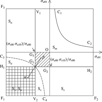
 ${\it\sigma}_{a01}<-|\overline{A}_{s}|^{-2}{\it\sigma}_{a00}={\it\sigma}_{a00}{\it\sigma}_{s10}/{\it\sigma}_{s00}$
(region
 $\text{F}_{1}\text{F}_{2}\text{H}_{2}\text{H}_{1}$
in figure 6), otherwise unstable. Similarly, the antisymmetric single-mode solution
 $$\begin{eqnarray}|\overline{A}_{s}|=0,\quad |\overline{A}_{a}|=\sqrt{-\frac{{\it\sigma}_{a00}}{{\it\sigma}_{a10}}},\quad {\it\mu}_{a}={\it\mu}_{a00}+|\overline{A}_{a}|^{2}{\it\mu}_{a10}={\it\mu}_{a00}-\frac{{\it\mu}_{a00}{\it\sigma}_{a10}}{{\it\sigma}_{a10}}\end{eqnarray}$$
exists in the whole region and stable in
 $\text{F}_{1}\text{V}_{2}\text{V}_{1}\text{F}_{3}$
.
Expected stable equilibrium solutions:
 $\text{S}_{s}$
, symmetric single-mode solution;
 $\text{S}_{a}$
, antisymmetric single-mode solution;
 $\text{S}_{m}$
, mixed-mode solution.

The amplitudes and frequencies are obtained for the mixed-mode solution as
 $$\begin{eqnarray}\left.\begin{array}{@{}l@{}}|\overline{A}_{s}|=\displaystyle \sqrt{-\frac{{\it\sigma}_{s00}{\it\sigma}_{a10}-{\it\sigma}_{a00}{\it\sigma}_{s01}}{{\it\sigma}_{s10}{\it\sigma}_{a10}-{\it\sigma}_{s01}{\it\sigma}_{a01}}},\quad {\it\mu}_{s}={\it\mu}_{s00}+|\overline{A}_{s}|^{2}{\it\mu}_{s10}+|\overline{A}_{a}|^{2}{\it\mu}_{s01},\\ |\overline{A}_{a}|=\displaystyle \sqrt{-\frac{{\it\sigma}_{a00}{\it\sigma}_{s10}-{\it\sigma}_{s00}{\it\sigma}_{a01}}{{\it\sigma}_{s10}{\it\sigma}_{a10}-{\it\sigma}_{s01}{\it\sigma}_{a01}}},\quad {\it\mu}_{a}={\it\mu}_{a00}+|\overline{A}_{a}|^{2}{\it\mu}_{a10}+|\overline{A}_{s}|^{2}{\it\mu}_{a01}.\end{array}\right\}\end{eqnarray}$$
The mixed mode exists if
 $({\it\sigma}_{s00}{\it\sigma}_{a10}-{\it\sigma}_{s01}{\it\sigma}_{a00})({\it\sigma}_{s10}{\it\sigma}_{a10}-{\it\sigma}_{s01}{\it\sigma}_{a01})<0$
and if
 $({\it\sigma}_{s10}{\it\sigma}_{a00}-{\it\sigma}_{s00}{\it\sigma}_{a01})({\it\sigma}_{s10}{\it\sigma}_{a10}-{\it\sigma}_{s01}{\it\sigma}_{a01})<0$
i.e. in
 $\text{F}_{1}\text{C}_{4}\text{G}_{1}\text{C}_{3}$
and
 $\text{G}_{1}\text{H}_{2}\text{C}_{2}\text{C}_{1}\text{V}_{1}$
in figure 6. Two eigenvalues for the mixed-mode solution are obtained as
 $$\begin{eqnarray}{\it\zeta}=|\overline{A}_{s}|^{2}{\it\sigma}_{s10}+|\overline{A}_{a}|^{2}{\it\sigma}_{a10}\pm \sqrt{\left(|\overline{A}_{s}|^{2}{\it\sigma}_{s10}-|\overline{A}_{a}|^{2}{\it\sigma}_{a10}\right)^{2}+4|\overline{A}_{s}|^{2}|\overline{A}_{a}|^{2}{\it\sigma}_{s01}{\it\sigma}_{a01}},\end{eqnarray}$$
and the other two are trivial. As
 ${\it\sigma}_{s01}<0$
and
 ${\it\sigma}_{a01}<0$
, the mixed solution is stable in
 $\text{G}_{1}\text{H}_{2}\text{C}_{2}\text{C}_{1}\text{V}_{1}$
and unstable in
 $\text{F}_{1}\text{C}_{4}\text{G}_{1}\text{G}_{3}$
.
To summarize, if we confine our discussion to the cases of
 ${\it\sigma}_{s01}<0$
and
 ${\it\sigma}_{a01}<0$
as well as
 ${\it\sigma}_{s10}<0$
and
 ${\it\sigma}_{a10}<0$
as the present numerical calculations show, the mixed-mode solution is stable and the two single-mode solutions are unstable in the region
 $\text{G}_{1}\text{G}_{2}\text{O}\text{G}_{3}$
, and vice versa in
 $\text{F}_{1}\text{V}_{2}\text{G}_{1}\text{H}_{1}$
. Furthermore, the trace of the coefficients moves along a line such as indicated by
 ${\it\alpha}{\it\beta}$
from
 $\text{G}_{1}\text{G}_{2}\text{O}\text{G}_{3}$
to
 $\text{F}_{1}\text{V}_{2}\text{G}_{1}\text{H}_{1}$
, or from
 $\text{F}_{1}\text{V}_{2}\text{G}_{1}\text{H}_{1}$
to
 $\text{G}_{1}\text{G}_{2}\text{O}\text{G}_{3}$
inevitably going through the point
 $\text{G}_{1}$
, though the line
 ${\it\alpha}{\it\beta}$
in figure 6 is schematic. Thus we arrive at a conclusion that the stability of the mixed-mode solution exchanges with both the two single-mode solutions simultaneously. This conclusion is valid to all cases of two-mode nonlinear interactions as far as the two amplitudes are governed by (2.38) with coefficients of
 ${\it\sigma}_{s01}<0$
and
 ${\it\sigma}_{a01}<0$
as well as
 ${\it\sigma}_{s10}<0$
and
 ${\it\sigma}_{a10}<0$
, i.e. to all cases of double Hopf bifurcations.
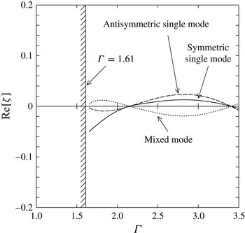
We demonstrate the changes of stability of the mixed mode and the two single modes of solutions in figure 7 for
 $\mathit{Re}=60$
where the real parts of
 ${\it\zeta}$
,
 $\text{Re}[{\it\zeta}]$
, for the three modes are depicted as functions of
 ${\it\Gamma}$
, where the solid and broken lines indicate the growth rate of disturbance for the symmetric and antisymmetric single modes solution, respectively, and the dotted line for the mixed-mode solution. At
 $\mathit{Re}=60$
, both the symmetric and antisymmetric modes of disturbance grow due to instability of the steady symmetric flow for
 ${\it\Gamma}\geqslant 1.61$
, and hence we depicted
 $\text{Re}[{\it\zeta}]$
only in the range of
 $1.61\leqslant {\it\Gamma}\leqslant 3.5$
. In this figure, the mixed mode equilibrium solution is stable and the two single-mode solutions are unstable in the range of
 $2.10\leqslant {\it\Gamma}\leqslant 3.41$
, while the mixed-mode solution is unstable and the two single-mode solutions are stable outside the range. Thus, we can confirm our conclusion derived above that the stability of the mixed-mode solution exchanges with both the two single-mode solutions simultaneously.
Growth rate
 ${\it\zeta}_{r}$
of equilibrium solutions depending on the gap ratio,
 $\mathit{Re}=60$
: solid line, symmetric single-mode solution; broken line, antisymmetric single-mode solution; dotted line, mixed-mode solution.

Thus we have evaluated the equilibrium amplitude and examined the stability for the three modes of solutions and subdivided the region IV of figure 4 into IV-1 and IV-2 as in figure 8. In subregion IV-1, the two single-mode solutions are stable and the mixed-mode solution is unstable, where the equilibrium state is not uniquely determined. On the other hand, the region IV-2 indicates that only the mixed-mode solution is possible and the equilibrium state is uniquely determined through the nonlinear interactions between the two modes of disturbance.
Expected stable equilibrium solutions: solid line, symmetric mode; broken line, antisymmetric mode; dotted line, boundary between IV-1 and IV-2; I, steady symmetric flow; II, antisymmetric single-mode solution; III, symmetric single-mode solution; IV-1, symmetric or antisymmetric single-mode solution; IV-2, mixed-mode solution.

5. Numerical simulation
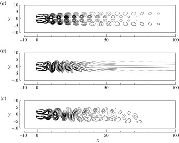
We have executed numerical simulations and obtained various flow fields in the range of
 $40\leqslant Re\leqslant 80$
and
 $1\leqslant {\it\Gamma}\leqslant 3.5$
, among which we will show three typical flow patterns at
 $\mathit{Re}=60$
in figure 9(a–c) for
 ${\it\Gamma}=2.0$
and 2.5 which lies on each side of
 ${\it\Gamma}_{c}$
. In these figures, vorticity distributions are depicted by contour lines, where dark and light lines indicate positive and negative vorticity, respectively. In the case of
 ${\it\Gamma}=2.0$
, we obtained two different flows as the equilibrium state at the same Reynolds number of
 $\mathit{Re}=60$
as shown in figure 9(a,b), either of which is realized depending upon the initial condition adopted. The flow pattern in figure 9(a) is obtained when the flow field
 $(\overline{{\it\psi}}+0.1\widetilde{{\it\psi}}_{s},\overline{{\it\omega}}+0.1\widetilde{{\it\omega}}_{s})$
is adopted as the initial condition. This flow occurs when the symmetric mode of disturbance attains its equilibrium state overwhelming the antisymmetric mode. In this figure, vortices are shed in antiphase behind the two cylinders and the symmetric arrangement of double vortex streets is kept for a long distance downstream, each vortex having a distinct shape. While in-phase vortex shedding is observed as shown in figure 9(b) when the initial condition is taken as
 $(\overline{{\it\psi}}+0.1\widetilde{{\it\psi}}_{a},\overline{{\it\omega}}+0.1\widetilde{{\it\omega}}_{a})$
. This flow is realized when the antisymmetric single-mode solution becomes the equilibrium solution through the nonlinear interaction between the two modes. In this case, each couple of vortices having the same sign amalgamate into a larger one in a short distance such as
 $x\sim 10$
to form a single vortex street, and disappear losing their shapes at
 $x\sim 40$
. The flow field of figure 9(b) resembles the wake pattern behind a single flat rectangular cylinder, which is made from the two square cylinders by blocking the gap so as not to allow any stream between them, because the wake in figure 9(b) is an almost single vortex street resulting from amalgamation of the two in-phase vortex streets and comprising flattened vortices.
Flow fields (contour lines of vorticity),
 $\mathit{Re}=60$
: (a)
 ${\it\Gamma}=2.0$
, initial condition, the steady symmetric plus a symmetric mode of disturbance; (b)
 ${\it\Gamma}=2.0$
, initial condition, the steady symmetric flow plus an antisymmetric mode of disturbance; (c)
 ${\it\Gamma}=2.5$
, both initial conditions of the steady symmetric flow plus either symmetric or antisymmetric mode of disturbance leads to this flow pattern.

These flow characteristics were already observed by Williamson (Reference Williamson1985) in his visualization of the wake behind a pair of circular cylinders. He found that two different flow patterns are realized at
 $\mathit{Re}=200$
and
 ${\it\Gamma}=2.0$
, and that antiphase vortices keep its arrangement for a long distance downstream, while vortices shed in in-phase lose their shapes in a short distance and the two parallel vortex streets change into a large-scale combined wake. Thus, Williamson’s experiments as well as our numerical simulations prove validity of the present results derived from the weakly nonlinear stability analysis in the point that the solution is not uniquely determined but depends on the initial condition. Such dual flow patterns were reported also for two square cylinders by Agrawal, Djenidi & Antonia (Reference Agrawal, Djenidi and Antonia2006). Using the lattice Boltzmann method, they showed both in-phase and antiphase vortex shedding flows, similar to those presented in figure 9(a,b), appear for
 ${\it\Gamma}=2.0$
at
 $\mathit{Re}=73$
, although they describe that antiphase locking of vortices is seen at the beginning of simulation starting from rest and subsequently in-phase shedding of vortices occurs. Their numerical simulation also realized both flow patterns even for
 ${\it\Gamma}=2.5$
at
 $\mathit{Re}=73$
, which is consistent with our conclusion because the parameter is located in region IV-1 in figure 8.
The flow pattern shown in figure 9(c) appears in the case of
 ${\it\Gamma}=2.5$
and
 $\mathit{Re}=60$
when the mixed-mode solution equilibrates through the two mode interaction so that the flow is realized independently of the initial condition because the mixed-mode solution is uniquely determined as well. In this case, vortices are shed in antiphase forming two vortex streets just behind the cylinders, but their shapes and the arrangement are deformed in a short distance of
 $x\sim 20{-}30$
to become so complicated that we cannot identify them with one or two vortex streets. This is also consistent with the weakly nonlinear results in figures 5(b) and 8 which show that the asymmetric flow includes the two modes of disturbance with both finite amplitudes in the equilibrium state.
The deformation of the two in-phase vortex streets into a single street was explained by Williamson (Reference Williamson1985). He observed each pair of like-signed vortices rotate around one another in the two in-phase vortex streets to form a large-scale combined wake. On the other hand, Hussain (Reference Hussain1986), Kolář, Lyn & Rodi (Reference Kolář, Lyn and Rodi1997) and Zhou, Zhang & Yiu (Reference Zhou, Zhang and Yiu2002) raised an explanation that the inner vortices with opposite sign strongly interact to diminish cancelling with each other, and yield a single vortex street. These two phenomenological explanations are still controvertible. Note that in these phenomenological explanations, vortices are assumed to keep their strengths and shapes for long time or for long distance. However, at small Reynolds numbers of approximately 50–80, vortices decay soon only advected in several times the cylinder diameter as Mizushima et al. (Reference Mizushima, Hatsuda, Akamine, Inasawa and Asai2014) showed. Our linear stability analysis shows that the rapid decay of the two in-phase vortex street is due to absence of the driving mechanism because the vortices will decay out without any forcing mechanism at such small Reynolds numbers, and the eigenfunction to induce the vortices are very weak beyond
 $x\sim 50$
as depicted in figure 3(c). A similar decay phenomenon of a vortex street was reported for the flow behind a rectangular cylinder with an aspect ratio of 0.2, where the rapid decay of the vortex street was successfully explained by the pattern of the eigenfunction similar to figure 3(c) (see Mizushima et al. (Reference Mizushima, Hatsuda, Akamine, Inasawa and Asai2014) for more details). Our explanation is an alternative and does not contradict phenomenological ones because various explanations can be possible for a single phenomenon.
We will further compare the numerical simulation data with the results of the weakly nonlinear stability analysis by evaluating the physical quantities corresponding to
 $A_{s}$
and
 $A_{a}$
from simulation data. We define the
 $y$
-component of velocity at
 $\text{P}_{1}$
and
 $\text{P}_{2}$
as
 $v_{1}$
and
 $v_{2}$
, and then consider their difference and the sum:
 $(v_{1}-v_{2})/2$
and
 $(v_{1}+v_{2})/2$
. We collect the time history data of
 $(v_{1}-v_{2})/2$
and
 $(v_{1}+v_{2})/2$
during approximately 100 of oscillation periods and transform them into Fourier spectra via a fast Fourier transform (FFT) routine. The resultant Fourier spectra of
 $(v_{1}-v_{2})/2$
and
 $(v_{1}+v_{2})/2$
have a sharp peak at
 ${\it\mu}_{s}$
and
 ${\it\mu}_{a}$
, respectively, only which we extract through a narrow-path filter and make an inverse Fourier transformation to obtain symmetric and antisymmetric modes of disturbance
 $v_{s}(t)$
and
 $v_{a}(t)$
. These physical quantities
 $v_{s}(t)$
and
 $v_{a}(t)$
correspond to
 $A_{s}(t)$
and
 $A_{a}(t)$
in the weakly nonlinear stability theory. Note that our definitions of
 $A_{s}(t)$
and
 $A_{a}(t)$
ensure this comparison because no symmetric component is included in
 $A_{a}(t)$
.
We depict the oscillation amplitudes
 $a_{s}$
and
 $a_{a}$
of
 $v_{s}(t)$
and
 $v_{a}(t)$
together with
 $|A_{s}|$
and
 $|A_{a}|$
for
 ${\it\Gamma}=2.0$
and 2.5 in figure 10(a,b), where the dark and the light lines indicate the amplitudes obtained from the the weakly nonlinear stability analyses and numerical simulations, respectively, and both the data are labelled as
 $|A_{s}|$
and
 $|A_{a}|$
to save space. In the case of
 ${\it\Gamma}=2.0$
(figure 10
a), the amplitudes
 $a_{s}$
and
 $a_{a}$
are shown to arise via Hopf bifurcations from the steady symmetric flow, whose bifurcation points are
 $\mathit{Re}_{s}=53.77$
and
 $\mathit{Re}_{a}=47.98$
. These critical Reynolds numbers agree with those determined in the linear stability analyses. Thus, dual stable solutions are reconfirmed also in this figure so that the equilibrium solution is not determined uniquely, but one of the two possible solutions is realized depending upon the initial condition. The magnitude of
 $a_{s}$
and
 $a_{a}$
agree with
 $|A_{s}|$
and
 $|A_{a}|$
obtained from weakly nonlinear stability analyses for the two single-mode solutions. Note that the amplitudes
 $a_{s}$
and
 $a_{a}$
for the mixed-mode solution cannot be obtained in numerical simulation because the solution is unstable and unattainable in the time marching scheme used in our simulation.
Bifurcation diagrams obtained by the numerical simulations which are compared with the weakly nonlinear stability results: solid line, stable; broken line, unstable; dark line, weakly nonlinear stability analysis; light line, numerical simulation; (a)
 ${\it\Gamma}=2.0$
; (b)
 ${\it\Gamma}=2.5$
.

For the case of
 ${\it\Gamma}=2.5$
, only the symmetric single-mode solution exists and it is stable in the range of
 $49.40\leqslant Re\leqslant 51.79$
, while all three solutions, two single-mode and the mixed solutions, are possible for
 $\mathit{Re}\geqslant 51.79$
although both of the single-mode solutions are unstable and only the mixed-mode solution is stable as shown in figure 10(b). Although the two single-mode solutions are unstable, we can numerically evaluate the equilibrium amplitude
 $a_{s}$
of the symmetric single-mode solutions by utilizing the symmetry conditions of
 ${\it\psi}(x,-y)=-{\it\psi}(x,y)$
and
 ${\it\omega}(x,-y)=-{\it\omega}(x,y)$
. However, we have no appropriate method to evaluate the equilibrium amplitude
 $a_{a}$
for the antisymmetric single-mode solution. The equilibrium value of
 $a_{s}$
evaluated from the coupled amplitude equations is seen to well approximate the numerical results for the symmetric single-mode solution in figure 10(b). The mixed-mode solution consisting of the symmetric and antisymmetric components
 $|A_{s}|$
and
 $|A_{a}|$
, which is the only stable solution in the range of
 $\mathit{Re}>51.79$
, deviate from the simulation results significantly for
 $\mathit{Re}\gtrsim 65$
, which may be a limit of applicability of the weakly nonlinear stability theory. Thus, we found that the equilibrium state is uniquely determined to be the mixed-mode solution irrespective of the initial condition in this range.
6. Concluding remarks
The steady symmetric flow pas a pair of square or circular cylinders is a solution of the governing equation for the flow dynamics irrespective of the Reynolds number, but becomes unstable to antisymmetric or symmetric oscillatory modes of disturbance depending on the gap ratio between the cylinders. The antisymmetric mode of disturbance is most unstable for smaller gap ratios than a threshold value of
 ${\it\Gamma}_{c}=2.25$
and yields two in-phase vortex streets, which diminish in a short distance behind the cylinders into a single vortex street as observed behind a flat rectangular cylinder, and then the vortex street disappears further downstream. On the other hand, the symmetric mode becomes the most unstable for larger gap ratios than the threshold value, leading to a symmetric oscillatory flow patterns with double Kármán vortex streets, which persists through a long distance far downstream. Thus, the two modes interchange their role of the most unstable mode with each other at the threshold gap ratio
 ${\it\Gamma}_{c}$
. Around the threshold gap ratio, both modes grow and through nonlinear interactions of the two modes of disturbance, the equilibrium state is established.
There have been so many reports in which the flow patterns at the equilibrium state are classified into several categories, where the authors assumed involuntarily that the state will be determined uniquely independent of the initial condition although multiple stable states have been already reported by Williamson (Reference Williamson1985). Our objective is to elucidate the nonlinear interactions of the two modes of disturbance when both modes of disturbance grow and to find the dynamics in which the equilibrium state is attained. Hence, we formulated a couple of amplitude equations to describe the nonlinear interactions. By solving the equilibrium solutions of the coupled amplitude equations and analysing the linear stability of the equilibrium solutions, we arrived at a conclusion that there are indeed cases where the equilibrium state is not unique but multiple stable states are possible. We found that in a confined parameter region a mixed-mode solution comprising the two modes of disturbance gives a unique equilibrium state. Outside the region either mode overwhelms the other to survive by itself and it depends on the initial condition which of symmetric or antisymmetric mode survives. Hence, the equilibrium solution is not uniquely determined in this region. More precisely, if we consider a case of gap ratio smaller than the thresholds value for instance, the antisymmetric mode of disturbance becomes to grow at a critical Reynolds number, say
 $\mathit{Re}_{c1}$
, and the symmetric mode of disturbance also becomes a growing mode at a small excess than
 $\mathit{Re}_{c1}$
, say
 $\mathit{Re}_{c2}$
. If we consider the case where both modes are growing at a Reynolds number larger than
 $\mathit{Re}_{c2}$
, the antisymmetric mode of disturbance, which grows at lower Reynolds number, may hold predominance and give the equilibrium state suppressing the symmetric mode if the Reynolds number increases quasi-statically, because the antisymmetric mode has a finite amplitude when the symmetric mode begins to grow. Needless to say, the symmetric mode can grow suppressing the antisymmetric mode when some relevant or suitable fluctuation is given in the flow field. Such a nonlinear competition between the two modes are drawn in the phase diagrams in figure 5(a,b). The diagrams show the dynamics of the nonlinear interactions between the two modes, or the mechanism to determine the equilibrium state through the nonlinear interactions.
We note that the conclusion that the two single-mode solutions exchange stability simultaneously with the mixed mode is generally applicable also to other flows than the wake behind two side-by-side cylinders, as far as the amplitudes of the two modes are described by the coupled amplitude equation derived in the present paper, i.e. in the cases of double Hopf bifurcation without any resonance. Hence, when any flow becomes unstable to two oscillatory modes of disturbance, there are three candidates for the equilibrium solution such that either of symmetric and antisymmetric single-mode solutions survives, or a mixed-mode solution attains its equilibrium state. If the mixed-mode solution is found, the resultant nonlinear equilibrium state is unique. Otherwise, either of the two single-mode solutions is probable and the equilibrium state is not unique but depends on the initial condition.
Acknowledgement
The authors express their cordial thanks to Professor K. Fujimura at Tottori University for his valuable advice on the stability of the equilibrium solutions of the coupled amplitude equations.