1 Introduction
Rotor systems are used in many engineering contexts as propulsion and renewable energy devices and a deeper insight on the physical processes that drive their performance, efficiency and low impact on the environment is of utmost importance. One of the most intriguing aspect of rotor functioning is wake destabilization, because this mechanism is associated with efficiency loss, amplification of vibratory and fatigue loads and generated noise. In fact, the wake of a marine propeller alters rudder loads (and then control capabilities of the ship) and determines vibrations transmitted to the hull. Similarly, rotor wake instabilities can affect flight control characteristics for helicopters (because of unsteady loads on the fuselage and modified inflow at the tail rotor (Conlisk Reference Conlisk2001)) or wind turbine performances in wind farms (because a turbine in the wake of other rotor can experience strongly altered inflow, with a reduced velocity and increased turbulence intensity). In particular, for large wind turbines installed in wind farms, wake instability leads to reduced power production and increases fatigue loading, turbulence and noise. All these reasons explain the importance of understanding the connection between the geometry and operating conditions of rotors with wake transition and instability (Sørensen Reference Sørensen2011).
The wake generated by a rotor is characterized by vortical structures which evolve in a complex fashion. In particular, intense tip vortices are observed from each blade, together with root vortices and weaker structures shed along the trailing edge; the vortical system is completed by a strong, longitudinal vortex from the hub. The evolution of the wake during the downstream convection is dominated by the mutual interaction of these structures and by their intensity. In turn, these depend on the shape of the rotor (number of blades, chord, geometric pitch) and its operative conditions (i.e. the inflow).
Earlier theoretical studies on wake stability focused on the dynamics of the helical tip vortices (Widnall Reference Widnall1972; Wood & Boersma Reference Wood and Boersma2001) or synthesized the wake with the simple Joukowski’s model (system of tip vortices and hub vortex Gupta & Loewy (Reference Gupta and Loewy1974), Okulov (Reference Okulov2004)). Although the peculiar mechanisms of the vortical system are captured by these simple models (short and long wave destabilization of vortex filament due to self-induction and the leap-frog process), these representations gave an unconditionally unstable wake and were not able to explain the stable evolution observed by visualizations of wind turbine flows under certain operative conditions (Vermeer, Sørensen & Crespo Reference Vermeer, Sørensen and Crespo2003).
Experimental analysis of the wake of a marine propeller by means of particle image velocimetry (PIV) (Di Felice et al. Reference Di Felice, Di Florio, Felli and Romano2004) highlighted that the stable evolution of the wake was correlated with the blade vortex sheet, that prevented the transverse motions of the adjacent tip vortex and hub vortex; as soon as this structure was disrupted due to vortex interaction and turbulent diffusion, the tip and hub vortices experienced transverse motions giving onset to a complete destabilization. This result was confirmed analytically by the general stability theory developed by Okulov & Sørensen (Reference Okulov and Sørensen2007) that enhanced the Joukowski model with the superposition of a distribution of vorticity within the rotor slipstream in order to model the blade vortex sheet; by means of this model, the predicted operative conditions that generate a stable wake resulted in close agreement with the experiments. Moreover, the evolution of the blade vortex sheet determines different mechanisms of destabilization of the wake, depending on the spanwise distribution of the blade circulation, and the shape of the blade. In fact, for a blade loaded at the tip, such as the one considered in the experimental analysis of Felli, Camussi & Di Felice (Reference Felli, Camussi and Di Felice2011), the blade sheet is disrupted by the interaction with the preceding tip vortex; on the contrary, Kumar & Mahesh (Reference Kumar and Mahesh2017) observed that, in the case of a skewed blade moderately loaded at the tip, the leap-frog process of the tip vortices occurred after the complete roll up process of blade vortex sheet and its gradual distortion in the transverse plane.
The evolution of the rotor wake after the transition regime can be strongly affected by the dynamics of the hub vortex. The visualizations in Felli et al. (Reference Felli, Camussi and Di Felice2011) highlighted that the hub vortex destabilized with a spiral motion having the same period of the hub, and an amplitude increasing with the number of blades and the loading condition; moreover, it sustained the precession mechanism of the propeller slipstream, affecting also the mutual interaction of the outer structures. Stability analysis (Iungo et al. Reference Iungo, Viola, Camarri, Porté-Agel and Gallaire2013; Viola et al. Reference Viola, Iungo, Camarri, Porté-Agel and Gallaire2014) further showed that the dynamics of the hub vortex can be described by the superposition of modes associated with structures characterized by different temporal and spatial frequencies. The destabilization of the hub vortex was associated with a dominant mode, with a frequency lower than the rotor one; this low frequency mode was associated with the wake meandering process observed during experiments of wind/current turbines. This mechanism is fundamental for the overall efficiency of array configurations, because it may delay the wake recovery for the downstream turbines, therefore degrading the overall efficiency and increasing the fatigue loads.
The time and spatial scales of these processes depends on rotor loading (and hence, the magnitude of vorticity generated by each blade) and the characteristics of the inflow. Felli et al. (Reference Felli, Camussi and Di Felice2011) investigated the effects of blade loading on the stability of the tip vortices and it was found that the smaller the inter-spiral distance (that is, the higher the loading), the sooner instability occurs. The onset of instability is followed by a multi-step grouping mechanism of the tip vortices that leads to very specific frequencies in the Fourier analysis of the velocity signals in the wake. Moreover, Ashton et al. (Reference Ashton, Viola, Camarri, Gallaire and Iungo2016) highlighted that, depending on the loading of the rotor, the dominant unstable modes can change from single to double helix configuration. On the other hand, when the inflow is not aligned with the propeller axis, new mechanisms concur to characterize the wake dynamics: in particular, besides the tip/hub vortex system, the flow is characterized by the generation of secondary structures at the interface of the slipstream with the undisturbed flow and a tilted convection of the hub vortex with respect to the tip vortices as a consequence of the asymmetric propeller loading distribution (Di Mascio, Muscari & Dubbioso Reference Di Mascio, Muscari and Dubbioso2014).
Since the wake of a rotor is rich with many complex structures that evolve in a wide range of different length and temporal scales, modal analysis techniques are extremely attractive to address its complex dynamics. The intent of these techniques is to reduce the order of the problem by projecting high-dimensional data onto a lower-dimensional space and, then, to identify the essential features of the process in terms of dominant coherent structures in order to understand its stability and dynamical properties.
These approaches are equation free and data driven, namely they do not rely on the direct solution of the system of nonlinear partial differential equations that describe the spatio-temporal evolution of the system; instead, they can be profitably applied when time accurate data of the state variables of a system (either from experiments or numerical simulation) are available.
Moreover, their further indisputable strength is the fact that these approaches are used to develop low-order models; this feature complies with emerging trends of rotor system design, pursued to maximize the overall efficiency during the entire operative lifecycle of the system including off-design conditions (i.e. downstream turbines in a farm, marine propeller behind the hull in waves or manoeuvering).
The field of modal analysis is wide and include a large number of different approaches (Rowley & Dawson Reference Rowley and Dawson2017). The majority of these approaches are linear, in the sense that a given configuration can be obtained as a linear combination of a set of basis functions. Even so, these techniques are able to properly analyse nonlinear systems. In particular, proper orthogonal decomposition (POD), also known as Karhunen–Loéve decomposition, has been widely used as a model-order reduction technique for a wide range of applications; a complete review on this methods and its applications can be found in Berkooz, Holmes & Lumley (Reference Berkooz, Holmes and Lumley1993). It was firstly applied to fluid mechanics by Lumley (Reference Lumley1970) in the analysis of turbulent flow data for the identification of coherent structures. This method allows for the extraction of the most energetic coherent structures by diagonalizing the spatial correlation function matrix of the snapshots matrix, and ranks the structures according to their energy content.
The dynamic mode decomposition (DMD) algorithm, recently proposed by Schmid (Reference Schmid2010), approximates the modes of the so-called Koopman operator (Rowley et al. Reference Rowley, Mezic, Bagheri, Schlatter and Henningson2009) using a variant of the Arnoldi algorithm. DMD computes eigenvalues and eigenmodes of an approximate linear model and, without the explicit knowledge of the dynamic operator, it extracts frequencies, growth or decay rates and spatial structures for each mode, yielding physically understandable results in terms of spatial structures and their associated temporal evolution.
Similarities between POD and DMD have been highlighted in Schmid (Reference Schmid2010), Muld, Efraimsson & Henningson (Reference Muld, Efraimsson and Henningson2012) and Semeraro, Bellani & Lundell (Reference Semeraro, Bellani and Lundell2012) where it was also shown that DMD modes may be reconstructed from POD modes.
Systematic applications of modal analysis techniques for the synthesis of rotor wakes are mostly documented in the renewable energy research field. In Sarmast et al. (Reference Sarmast, Dadfar, Mikkelsen, Schlatter, Ivanelli, Sørensen and Henningson2014) POD and the DMD were employed to analyse the breakdown process of the tip vortices for a three bladed wind turbine reproduced by means of large eddy simulations (LES) and an actuator line method. Both approaches were able to identify the growth rate of travelling waves associated with long wave stability, (see Widnall Reference Widnall1972); these perturbations propagate along the spirals during their downstream convection and promote the out-of-phase interaction of consecutive spirals, leading to wake breakdown. An analytic formulation of the length of the wake up to destabilization, dependent on the loading condition of the turbine, was developed on the basis of the spatial growth rate of the travelling waves. Debnath et al. (Reference Debnath, Santoni, Leonardi and Iungo2017) performed both a modal analysis and a reduced-order modelling of the wake field, obtained by LES, generated by a three bladed wind turbine in isolated and realistic condition (with the inclusion of nacelle and tower) by means of POD and DMD. Results of these two works diverged significantly from each other, because in the realistic configuration the evolution of the tip vortices was completely disorganized due to strong interaction with the wake shed from the tower. This interaction prevented the organization of coherent vorticity in the core of the slipstream and led to a different breakdown mechanism of the tip vortices. For the isolated rotor, the instability of the tip vortices was driven by their splitting caused by the interaction with blob of vorticity formed by the roll up of the blade vorticity; conversely, for the realistic case, the destabilization was characterized by the leap-frog mechanism between consecutive tip vortices. Iungo et al. (Reference Iungo, Santoni-Ortiz, Abkar, Porté-Agel, Rotea and Leonardi2015) and Bastine et al. (Reference Bastine, Vollmer, Wächter and Peinke2018) developed prediction models of wind turbine wakes based on DMD-derived reduced-order modelling (ROM) embedded with a Kalman filter and POD coupled with temporal stochastic models, respectively.
On the contrary, in marine propeller flows this kind of approach is still mostly used as a post-processing tool. By means of POD applied to PIV measurements of the flow for a propeller operating in the typical shear flow caused by an upstream hull, Paik et al. (Reference Paik, Kim, Lee and Lee2010) highlighted that the breakdown of the tip vortices always starts in the upper region of the slipstream; this is due to the fact that the vorticity distribution along the filaments is variable, as a consequence of the unsteady behaviour of the propeller, and the first merging occurs between chunks of adjacent tip vortices with higher circulation. Since measurements were carried out only in the longitudinal plane, the three-dimensional evolution of wake destabilization was not characterized. Felli, Falchi & Dubbioso (Reference Felli, Falchi and Dubbioso2015) performed a topological study of the noise sources generated in the near field of a marine propeller by means of POD analysis applied to tomographic PIV data. The flow field of a propeller attached to a submarine hull in crashback conditions was studied by LES and DMD in Kumar & Mahesh (Reference Kumar and Mahesh2015), where the flow mechanisms that generate high amplitude fluctuations of the side force in the vortex ring state and reverse flow were assessed identifying the DMD modes at the same frequency of the peaks in the spectrum of the load.
In the present work both POD and DMD techniques are applied to the analysis of the wake past a marine propeller achieved by numerical simulations in Muscari, Di Mascio & Verzicco (Reference Muscari, Di Mascio and Verzicco2013). The geometry is given by the INSEAN E779A propeller, which is a four blade, medium solidity propeller, designed with no skew and rake, operating in pure axial flow open water condition. This test case has been chosen for several reasons: it deals with a relatively simple geometry (a propeller in open water) and yet has a relevant engineering importance. Moreover, it is the same geometry used in the experimental work by Felli et al. (Reference Felli, Camussi and Di Felice2011), where the evolution of the tip and hub vortices of the propeller were studied in a water tunnel. Both a moderate and a highly loaded conditions (
 $J=0.71$
and
 $J=0.38$
) are analysed. These two conditions are characterized by different destabilization of the wake and different nature of the interaction between vortex structures. The application of the two reduced-order analysis allows for the identification of the most energetic modes, of those that play a dominant role in the inception of the destabilization and/or drive the dynamics of the wake after the destabilization starts. While the output of POD is a modal basis sorted according to their relative importance, it is not trivial to identify, solely from inspection, a subset of DMD modes that has the greatest influence on the flow dynamics. Therefore the sparsity promoting (SP) DMD technique proposed by Jovanović, Schmid & Nichols (Reference Jovanović, Schmid and Nichols2014) is implemented for the analysis of the snapshots matrix, in order to better capture the dominant features of the system by excluding those that weakly contribute to the flow dynamics.
In particular, we will try to associate a specific flow feature with each mode of the reconstruction and to assess the ability of these techniques to describe that mode in terms of spatial shape and characteristic frequency. The comparison of the methodologies is not aimed at assessing the reliability of one method over the other; as stressed in the above cited works on wind turbine wakes (Sarmast et al. Reference Sarmast, Dadfar, Mikkelsen, Schlatter, Ivanelli, Sørensen and Henningson2014; Debnath et al. Reference Debnath, Santoni, Leonardi and Iungo2017), the two approaches provide comparable results for the synthesis of the wake flow. Our goal is to exploit the two methods to help understand the key features of the evolution of the propeller wake.
2 Overview of numerical simulation
In this section an overview of the numerical simulation that yielded the snapshots used for the reduced-order analysis is presented. A full account of these contents can be found in Muscari et al. (Reference Muscari, Di Mascio and Verzicco2013).
2.1 Mathematical model
The numerical simulation of the flow field is performed by the integration of the Reynolds-averaged Navier–Stokes equations written in non-dimensional form in the frame of reference fixed to the propeller in terms of absolute velocity:
 $$\begin{eqnarray}\displaystyle \left\{\begin{array}{@{}l@{}}\unicode[STIX]{x1D735}\boldsymbol{\cdot }\boldsymbol{u}=0\\ \displaystyle \frac{\unicode[STIX]{x2202}\boldsymbol{u}}{\unicode[STIX]{x2202}t}+\unicode[STIX]{x1D74E}\times \boldsymbol{u}+\unicode[STIX]{x1D735}\boldsymbol{\cdot }[(\boldsymbol{u}-\unicode[STIX]{x1D74E}\times \boldsymbol{r})\otimes \boldsymbol{u}]+\unicode[STIX]{x1D735}p-\unicode[STIX]{x1D735}\boldsymbol{\cdot }\unicode[STIX]{x1D70F}=0,\end{array}\right. & & \displaystyle\end{eqnarray}$$
where
 $\boldsymbol{u}$
is the absolute velocity,
 $\unicode[STIX]{x1D74E}$
is the (constant) angular velocity,
 $\boldsymbol{r}=\boldsymbol{x}-\boldsymbol{x}_{0}$
is the position of point
 $\boldsymbol{x}$
with respect to
 $\boldsymbol{x}_{0}$
(origin of the non-inertial frame of reference),
 $p$
is the pressure,
 $\unicode[STIX]{x1D749}=\unicode[STIX]{x1D708}_{T}(\unicode[STIX]{x1D735}\boldsymbol{u}+\unicode[STIX]{x1D735}\boldsymbol{u}^{\text{T}})$
the stress tensor,
 $\unicode[STIX]{x1D708}_{T}=1/Re+\unicode[STIX]{x1D708}_{t}$
,
 $\unicode[STIX]{x1D708}_{t}$
being the turbulent viscosity calculated by the detached eddy simulation (DES) approach described in Spalart (Reference Spalart2009) and
 $Re$
the Reynolds number (later defined).
As boundary condition, at solid walls the velocity of the fluid is set equal to the local wall velocity, i.e.
 $\boldsymbol{u}=\unicode[STIX]{x1D74E}\times \boldsymbol{r}$
, at the inflow the velocity is set to the value of the undisturbed flow,
 $\boldsymbol{u}=\boldsymbol{U}_{\infty }$
, whereas at the outflow the velocity is extrapolated from inner points.
2.2 Numerical model
The numerical integration of the governing equations (2.1) is performed by means of an in-house solver. It is thoroughly described in Muscari et al. (Reference Muscari, Di Mascio and Verzicco2013) and the references cited therein, and we will briefly report here its main features for the sake of completeness.
The numerical algorithm is based on a finite volume technique with pressure and velocity co-located at cell centres. The computational domain is partitioned into structured blocks, each one subdivided into hexahedrons. Conservation laws are then applied to each hexahedron:
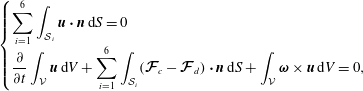 $$\begin{eqnarray}\displaystyle \left\{\begin{array}{@{}l@{}}\displaystyle \mathop{\sum }_{i=1}^{6}\int _{{\mathcal{S}}_{i}}\boldsymbol{u}\boldsymbol{\cdot }\boldsymbol{n}\,\text{d}S=0\\ \displaystyle \frac{\unicode[STIX]{x2202}}{\unicode[STIX]{x2202}t}\int _{{\mathcal{V}}}\boldsymbol{u}\,\text{d}V+\mathop{\sum }_{i=1}^{6}\int _{{\mathcal{S}}_{i}}(\boldsymbol{{\mathcal{F}}}_{c}-\boldsymbol{{\mathcal{F}}}_{d})\boldsymbol{\cdot }\boldsymbol{n}\,\text{d}S+\int _{{\mathcal{V}}}\unicode[STIX]{x1D74E}\times \boldsymbol{u}\,\text{d}V=0,\end{array}\right. & & \displaystyle\end{eqnarray}$$
where
 ${\mathcal{S}}_{i}$
is the
 $i$
th face of the generic finite volume
 ${\mathcal{V}}$
and the fluxes are decomposed into a convective part
 $\boldsymbol{{\mathcal{F}}}_{c}$
and a diffusive term
 $\boldsymbol{{\mathcal{F}}}_{d}$
.
A standard second-order centred scheme is used for the computation of viscous terms, whereas a centred fourth-order scheme has been applied for the computation of Eulerian terms. Because of the treatment of the viscous terms, the scheme is formally second-order accurate in space, although previous numerical experience proved that the use of a high-order approximation of the Eulerian terms can remarkably reduce the actual error.
The physical time derivatives are approximated by a second-order accurate, three-point backward finite difference formula. The resulting scheme is fully implicit in time and a dual time stepping approach is adopted for its integration.
The equations are discretized on a block structured grid with partial overlapping. This approach renders domain discretization and grid quality control much easier than with structured meshes with abutting blocks when dealing with complex geometries like the one under investigation. High performance computing is achieved by a hybrid shared (OMP) and distributed (MPI) memory parallelization.
3 Numerical set-up
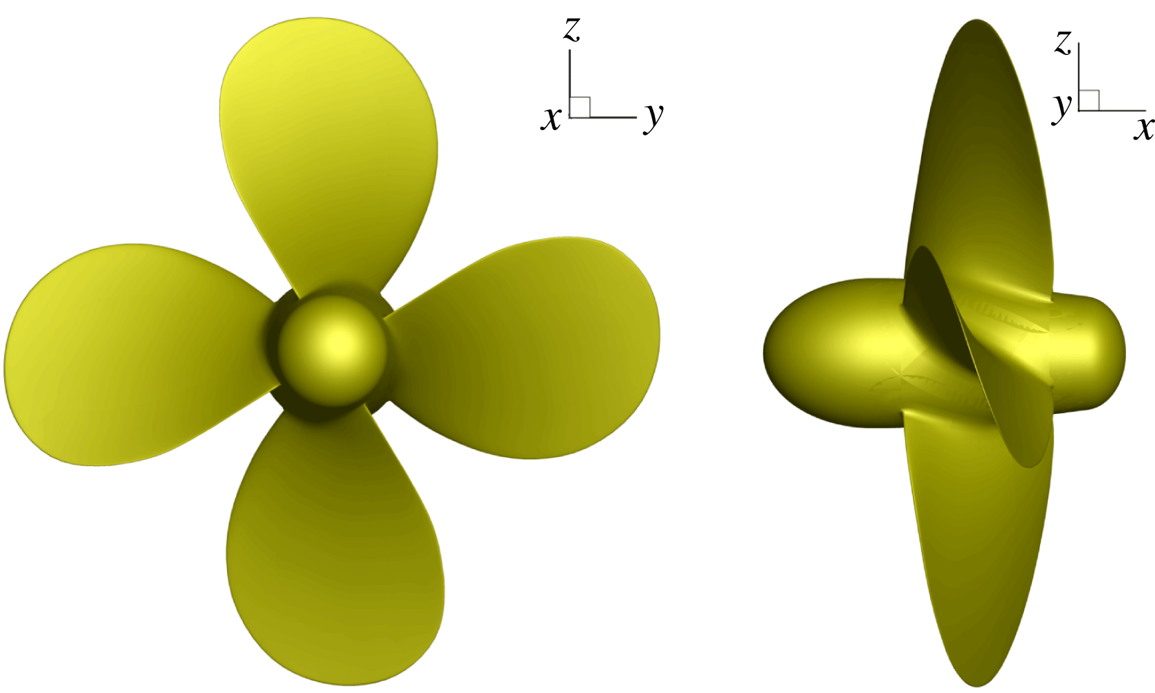
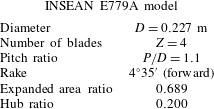
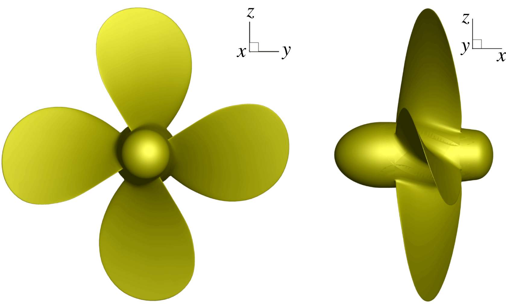
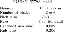
The propeller geometry chosen for this investigation is the INSEAN E779A model (Salvatore et al. Reference Salvatore, Pereira, Felli, Calcagni and Di Felice2006). It is a four blade, fixed-pitch, right-handed propeller, with a constant pitch distribution and a very low skew. In figure 1, back and side views of the propeller are shown, whereas its main geometrical features are reported in table 1.
Back and side views of the propeller model.
Propeller parameters.
In the numerical simulations, two different advance coefficients are considered, that is,
 $J=0.71$
representative of a stable wake condition (at least for the considered length of the wake field), and
 $J=0.38$
corresponding to an unstable wake characterized by the first phase of grouping mechanism of tip vortices observed in the experiments. The different advance coefficients,
 $J=U_{\infty }/nD$
, are obtained with a fixed value of the rotational speed of the propeller (
 $n=25\;\text{rps}$
) and varying the inflow velocity
 $U_{\infty }$
.
All quantities were cast in non-dimensional form by using as reference values the radius of the propeller (
 $L_{ref}=0.1135~\text{m}$
), the velocity of the blade tip (
 $U_{ref}=n\unicode[STIX]{x03C0}D\simeq 17.85~\text{m}~\text{s}^{-1}$
) and fluid density (
 $\unicode[STIX]{x1D70C}_{ref}=1000~\text{kg}~\text{m}^{-3}$
). Therefore, the reference time is
 $t_{ref}=L_{ref}/U_{ref}\simeq 0.0064~\text{s}$
and the non-dimensional period of revolution is
 $T=2\unicode[STIX]{x03C0}$
. The Reynolds number is the same of the physical experiment, i.e.
 $Re=U_{ref}L_{ref}/\unicode[STIX]{x1D708}=1.78\cdot 10^{6}$
. The non-dimensional time step was chosen to have a rotation of one degree for the propeller (
 $\text{d}t=2\unicode[STIX]{x03C0}/360\simeq 0.01745$
) per integration step.
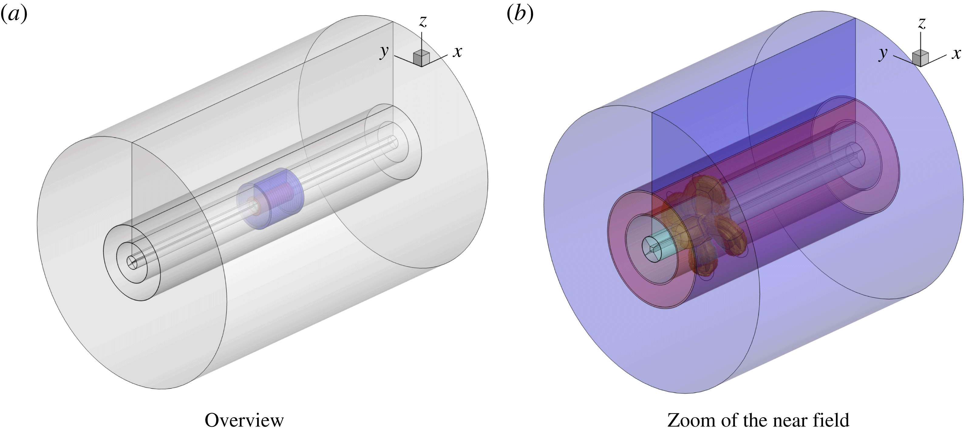
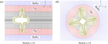
Figure 2 shows the building blocks of the mesh: for each blade and for both the fore and the aft parts of the hub, an ‘O-grid’ topology was chosen. The rest of the mesh is made up by concentric toroidal blocks that cover the whole computational domain. In order to give an idea of cell clustering, two slices in the planes
 $y=0$
and
 $x=0$
are reported in figure 3. In particular, the resolved part (finer grid) of the computational domain extends up to 4.4 radii downstream of the reference plane (
 $x=0$
) of the propeller, and this is the region within which we can expect to be able to properly capture the main flow features (tip and hub vortices).
Grid topology.

Details of the volume mesh.

The boundary layer is fully resolved, the first point being set at a distance from the wall such that
 $y^{+}<1$
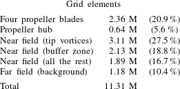
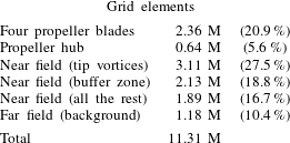
in wall unit. Apart from the blocks fitted around the geometry, most of the cells are placed in the toroidal block that is used to track the tip vortices; another external toroidal block is used as a buffer between the finer mesh near the propeller and the outer, coarser, background mesh. The different blocks sum up to a total of 11 M cells and their relative weight is detailed in table 2.
Finally, numerical uncertainty for the present test case was estimated using two grid levels, following the procedure reported in Roache (Reference Roache1997). Details and results can be found in Muscari et al. (Reference Muscari, Di Mascio and Verzicco2013).
For the modal analysis reported in the following, the results of the numerical simulations were interpolated on a single, structured, cylindrical block that extends from
 $0.5\,L_{ref}$
to
 $4.2L_{ref}$
in the longitudinal direction, and from 0 to
 $1.2L_{ref}$
in the radial direction. The dimensions of the toroidal block are
 $171\times 32\times 64$
cells in the longitudinal, radial, azimuthal directions, respectively, that correspond to cell dimensions
 $\unicode[STIX]{x0394}x\times \unicode[STIX]{x0394}r\times \unicode[STIX]{x0394}\unicode[STIX]{x1D703}=0.0218\times 0.0387\times 5.625^{\circ }$
. As a reference, the dimensions of the cells in the toroidal block, used for the DES, that comprises the motion of the tip vortices are
 $\unicode[STIX]{x0394}x\times \unicode[STIX]{x0394}r\times \unicode[STIX]{x0394}\unicode[STIX]{x1D703}=0.0146\times 0.0132\times 1.41^{\circ }$
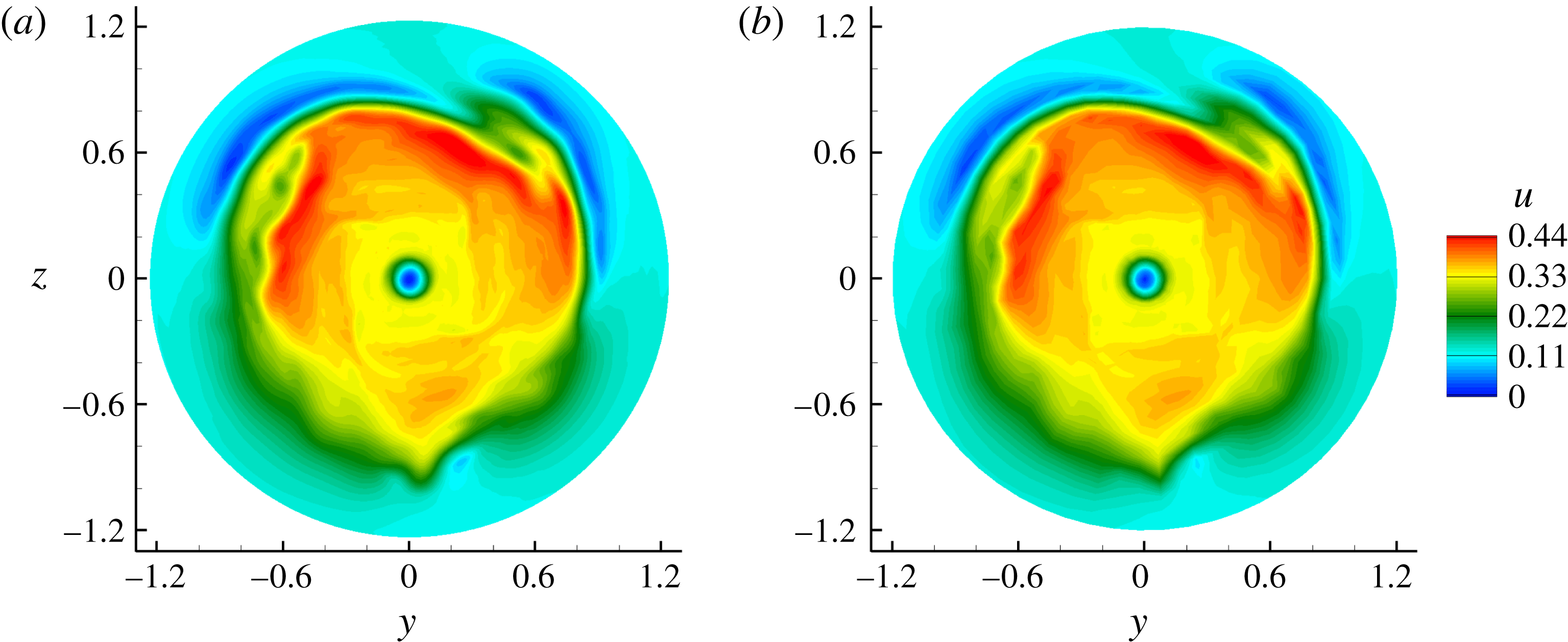
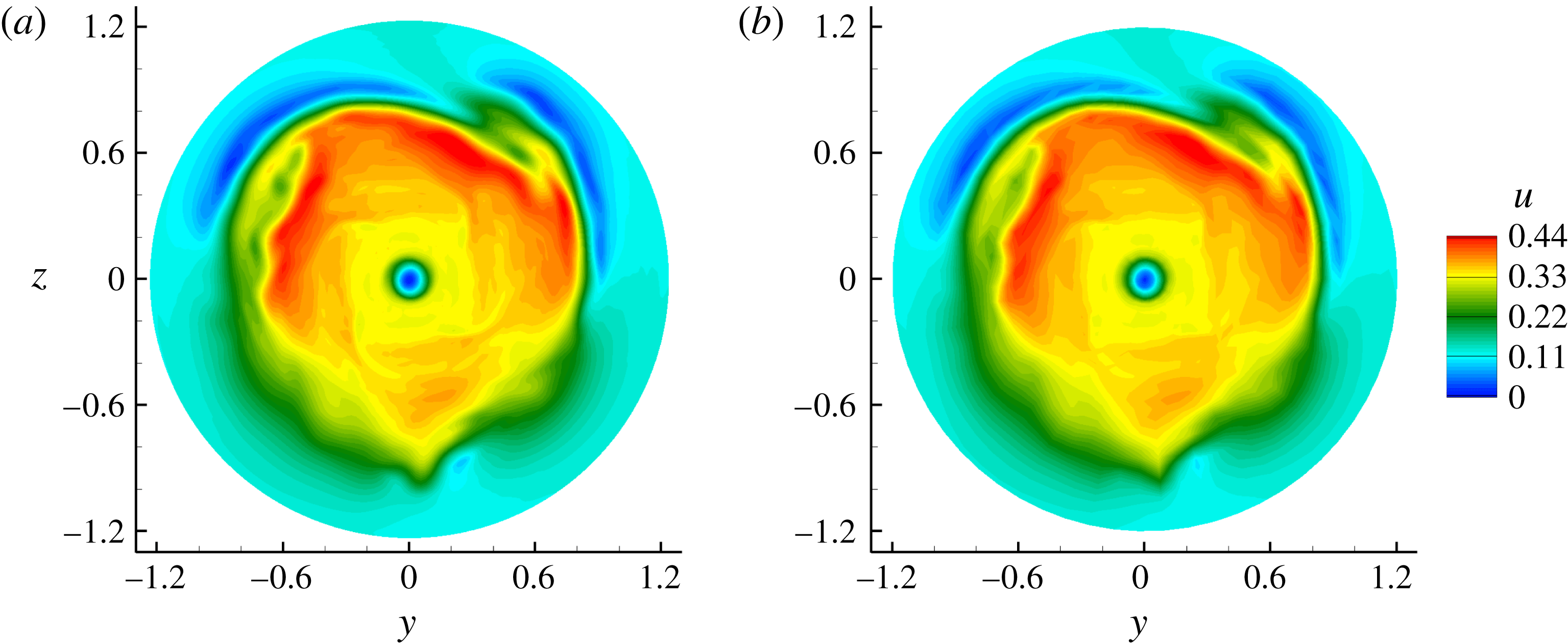
. Hence, the interpolation obviously results in a smoothing of the original dataset yielded by the numerical simulation, both because of the interpolation process itself and because the cells of the cylindrical block are bigger than those used for the DES. However, we expect that this smoothing concerns only the smallest scales of the flow, and does not impact on the results of the modal analysis concerning the biggest scales discussed in the following. For example, figure 4 compares transversal cuts of the longitudinal velocity field at
 $J=0.38$
extracted from the original data and from the interpolated data. Some differences in the finer details are visible between the two fields, but the overall solution is the same.
Case
 $J=0.38$
; transversal cuts of the longitudinal velocity field at
 $x=3$
. Original data (a), interpolated data (b).
Distribution of computational cells.
A database of 1200 snapshots is used with a time interval equal to six integration steps; hence, a time period equal to 20 propeller revolutions is covered. The resultant sampling frequency satisfy the Nyquist–Shannon criterion up to the seventh blade harmonic. Preliminary tests were performed to verify the convergence of the results.
Time sampling, like spatial interpolation, was necessary in order to limit the amount of memory requested by the modal analysis, in particular the DMD. The above choices, in terms of number of snapshots and cylindrical block dimensions, were the maximum allowed for a PC with 32 Gb of RAM used to perform the post-processing.
4 Description of the computed flow field
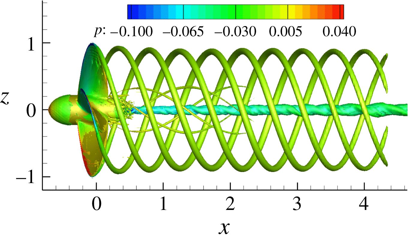
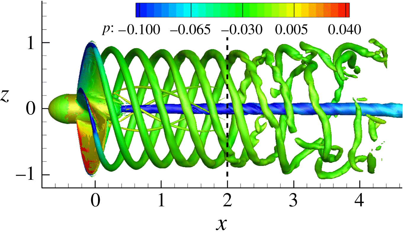
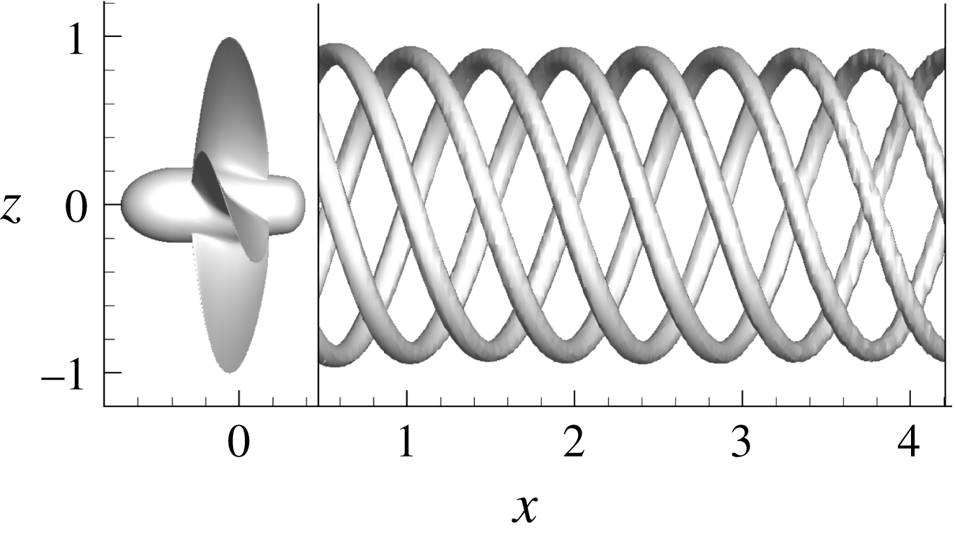
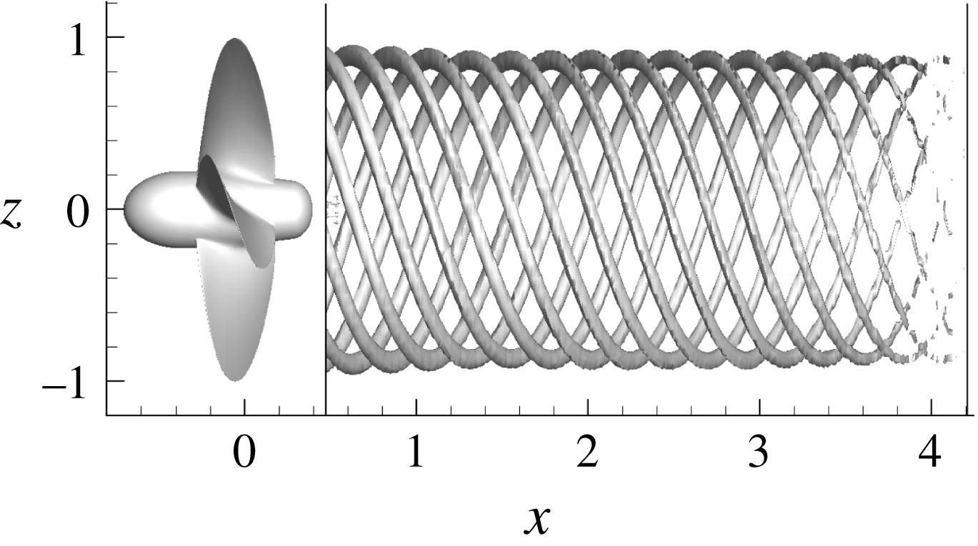
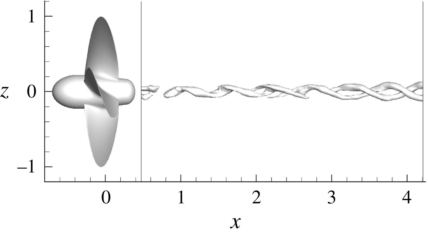
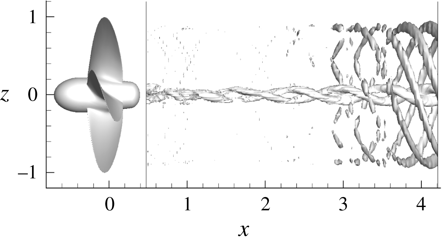
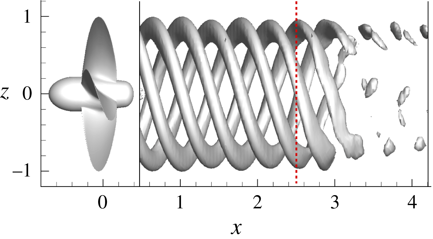
A brief overview of the wake field obtained by DES simulations for the two propeller loadings is described in figures 5 and 6, where the vortical structures are represented through isosurfaces of
 $\unicode[STIX]{x1D706}_{2}$
(Jeong & Hussain Reference Jeong and Hussain1995).
At
 $J=0.71$
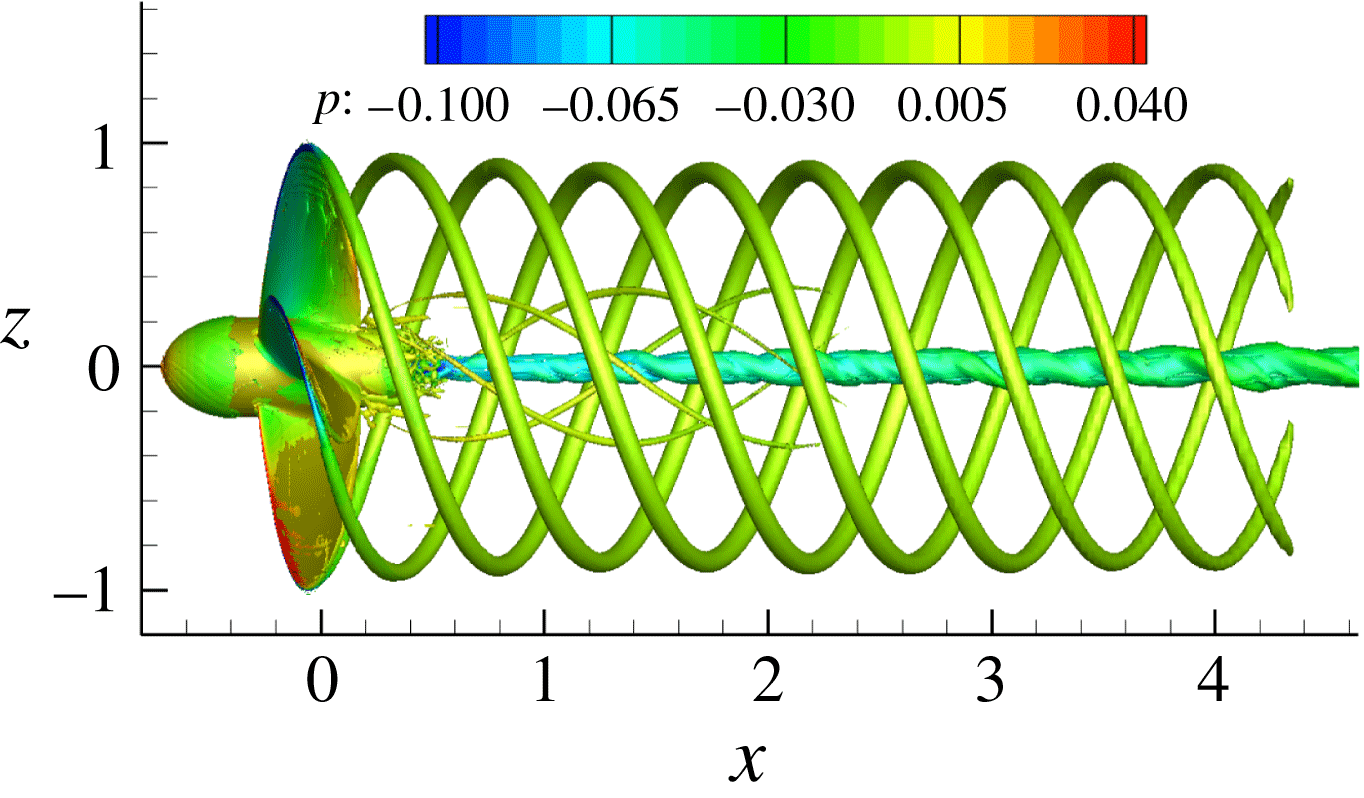
, the flow is characterized by the very regular succession of tip vortices detached from the blade tips and by an almost rectilinear hub vortex in the whole (resolved) computational domain. The tip vortices conserve their geometric characteristics (pitch and tip–tip distance) and do not present wave instabilities propagating along the vortex tubes. The stable nature of the flow up to the end of the computational domain is confirmed by the flow visualizations reported in Felli et al. (Reference Felli, Camussi and Di Felice2011).
At
 $J=0.38$
, two different regimes are evident, separated by the black dashed line (located at
 $x=2$
) in figure 6: close to the propeller the wake is stable, i.e. the pitch of the tip vortices and the mutual longitudinal distance is approximately constant. In the farthest zone, the vortical field is characterized by the mutual interaction between the tip vortices that leads to the leap-frogging mechanism described in Felli et al. (Reference Felli, Camussi and Di Felice2011) and, eventually, at their merging. As a consequence of this process, the geometry of each tip vortex deforms, as shown by the gradual variation of pitch angle and the appearance of perturbations along the filaments. With regard to the hub vortex, it is swept by a helical disturbance that grows with the distance. In both cases, the length of the computational domain is too short to entirely capture the complete hub vortex destabilization responsible of the precession/gyroscopic mechanism of the propeller slipstream observed in Felli et al. (Reference Felli, Camussi and Di Felice2011). The hub vortex precession grows moving downstream, and promotes the destruction of the coherent structures in the outer portion of the slipstream; recent studies in the field of wind turbines (Viola et al.
Reference Viola, Iungo, Camarri, Porté-Agel and Gallaire2014; Ashton et al.
Reference Ashton, Viola, Camarri, Gallaire and Iungo2016) clarified that the so called ‘meandering’ of the wakes has to be ascribed to the destabilization of the hub vortex.
Case
 $J=0.71$
; isosurface
 $\unicode[STIX]{x1D706}_{2}=-2$
.
Case
 $J=0.38$
; isosurface
 $\unicode[STIX]{x1D706}_{2}=-3$
.

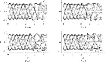
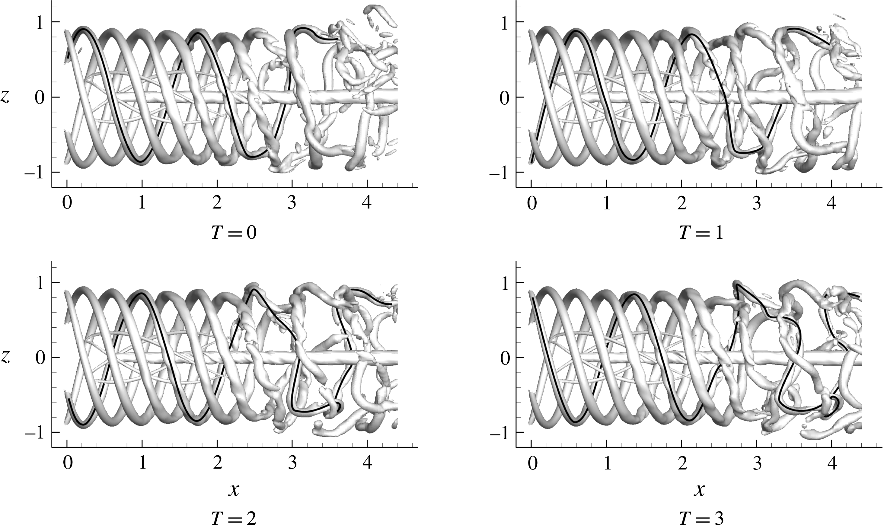
It is useful, for the following discussion, to focus on the temporal evolution of the vortical field in the destabilized region shown in the sequence of figure 7. First of all, it should be noted that the mutual interaction of the tip vortices alters the pitch distribution of the spirals that becomes strongly asymmetric during a period of revolution. This asymmetry is particularly evident for
 $x>3$
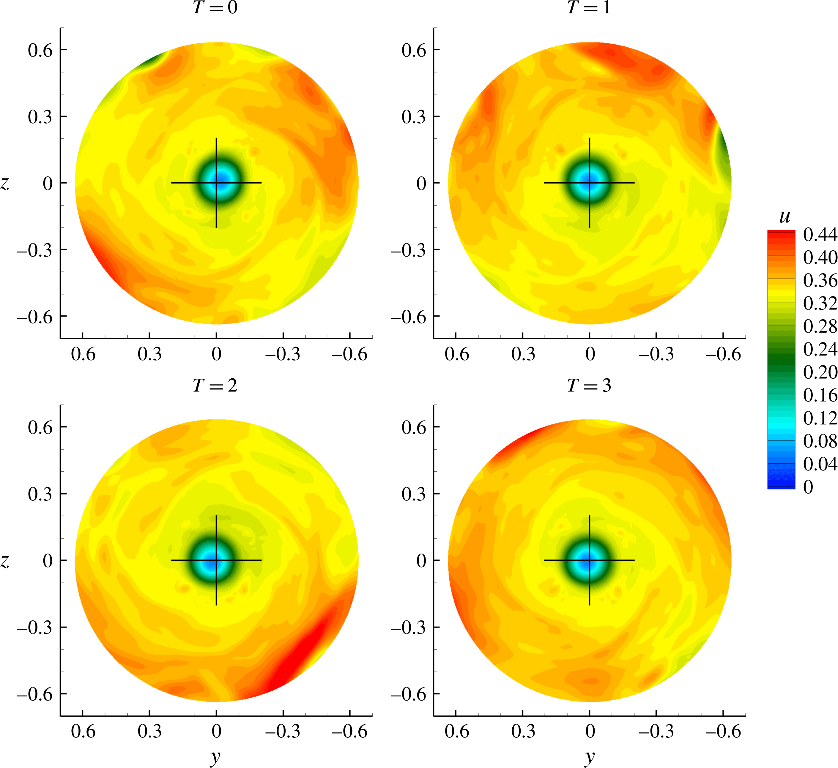
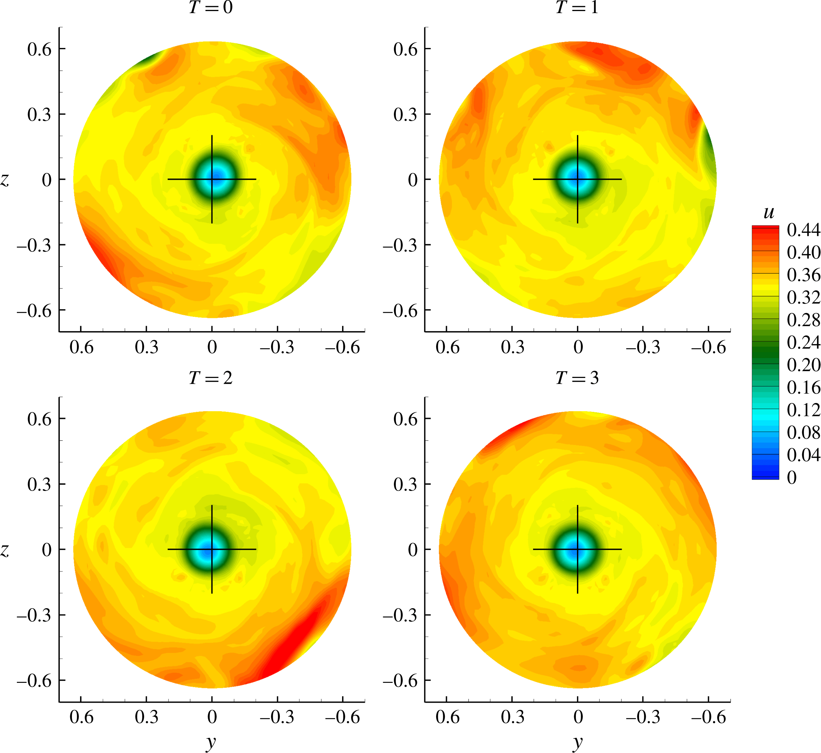
. Moreover, it can be noted that the hub vortex starts to oscillate after the destabilization of the outer structures of the slipstream, in agreement with the observations presented in Felli et al. (Reference Felli, Camussi and Di Felice2011). In particular, the coupling of two consecutive tip vortices and their variation of pitch are responsible for the onset of perturbations (that is, alterations of the induced velocity field) on the inner structures. This is visualized in figure 8 at a transverse section in the far field in terms of axial velocity. It is evident that the axial velocity is markedly asymmetric, the higher values caused by the increased induced velocity being located close to the merged tip vortices. The outer boundary of the slipstream is more rugged because of deformation, stretching and merging of the tip vortices; the deformation of the sectional area of the slipstream, together with the fluctuations of the hub vortex, induce a global precession motion to the vortex system (Felli et al.
Reference Felli, Camussi and Di Felice2011).
Case
 $J=0.38$
; evolution of the vortex field represented through the isosurface
 $\unicode[STIX]{x1D706}_{2}=-2$
. The four instants are separated by a quarter of a period of revolution. The black line helps to identify the same vortex filament during its evolution.
Axial velocity distribution inside the propeller slipstream at
 $x=4.2$
for
 $R\leqslant 0.65$
(i.e. the hub region; the black cross marks the position of the
 $x$
-axis.)
5 Modal decomposition
For the sake of completeness, the basic elements of POD and DMD are briefly recalled. Details can be found in the references cited in the corresponding sections.
5.1 Proper orthogonal decomposition
POD is a mathematical procedure that, given an ensemble of data preliminary removed of its mean, constructs a basis for the ensemble that is optimal, in the sense that no other decomposition of the same order captures an equivalent amount of kinetic energy. This technique uses a second-order statistics, namely the two-point correlation tensor, in order to extract organized large-scale structures from turbulent flows. The most energetic modes can be viewed as ‘dominant’ flow structures.
For our case, the data set is formed by the values of velocity and pressure in the
 $M=171\times 32\times 64$
nodes of the cylindrical block described above, for
 $N=1200$
instants, arranged to form a snapshot matrix:
 $$\begin{eqnarray}\displaystyle \unicode[STIX]{x1D64E}=[\boldsymbol{u}(\boldsymbol{x},t_{1}),\boldsymbol{u}(\boldsymbol{x},t_{2}),\ldots ,\boldsymbol{u}(\boldsymbol{x},t_{N})]. & & \displaystyle\end{eqnarray}$$
The POD modes are obtained by searching the
 $N$
functions
 $\unicode[STIX]{x1D753}_{i}$
that yield the best representation of the data set, that is that maximize the inner products
 $$\begin{eqnarray}\displaystyle I=\frac{\langle \boldsymbol{u}(\boldsymbol{x},t_{i}),\unicode[STIX]{x1D753}_{i}(\boldsymbol{x})\rangle ^{2}}{\Vert \unicode[STIX]{x1D753}_{i}(\boldsymbol{x})\Vert ^{2}}. & & \displaystyle\end{eqnarray}$$
The resolution of the maximization problem is performed using the calculus of variations and the result is an integral equation:
 $$\begin{eqnarray}\displaystyle \int _{\unicode[STIX]{x1D6FA}}\unicode[STIX]{x1D64D}(\boldsymbol{x},\boldsymbol{x}^{\prime })\unicode[STIX]{x1D753}(\boldsymbol{x}^{\prime })\,\text{d}\boldsymbol{x}^{\prime }=\unicode[STIX]{x1D706}\unicode[STIX]{x1D753}(\boldsymbol{x}). & & \displaystyle\end{eqnarray}$$
The kernel of this equation is the two-point correlation tensor
 $\unicode[STIX]{x1D64D}(\boldsymbol{x},\boldsymbol{x}^{\prime })$
that is
 $$\begin{eqnarray}\displaystyle \unicode[STIX]{x1D64D}(\boldsymbol{x},\boldsymbol{x}^{\prime })=\int _{0}^{\text{T}}\boldsymbol{u}(\boldsymbol{x},t)\boldsymbol{u}(\boldsymbol{x}^{\prime },t)\,\text{d}t. & & \displaystyle\end{eqnarray}$$
Since the autocorrelation tensor is self-adjoint and positive semidefinite (Holmes et al. Reference Holmes, Lumley, Berkooz and Rowley2012), the POD modes are orthogonal and satisfy the following orthonormality condition
 $$\begin{eqnarray}\displaystyle \int _{\unicode[STIX]{x1D6FA}}\unicode[STIX]{x1D753}_{n}(\boldsymbol{x})\unicode[STIX]{x1D753}_{m}(\boldsymbol{x})\,\text{d}\boldsymbol{x}=\unicode[STIX]{x1D6FF}_{nm}. & & \displaystyle\end{eqnarray}$$
The eigenvalues
 $\unicode[STIX]{x1D706}_{i}$
provide the energy contribution associated with the corresponding
 $i$
th POD mode
 $\unicode[STIX]{x1D753}_{i}$
; the energy percentage content of the
 $i$
th mode and the cumulative energy up to the
 $i$
th mode are defined as
 $$\begin{eqnarray}\displaystyle E_{i}=\frac{\unicode[STIX]{x1D706}_{i}}{\mathop{\sum }_{j=1}^{N}\unicode[STIX]{x1D706}_{j}},\quad E_{i}^{cum}=\mathop{\sum }_{k=1}^{i}E_{k}. & & \displaystyle\end{eqnarray}$$
One of the major benefits of POD comes from its ability to sort the obtained modal basis in relation to their relative importance; in this way the dominant features may be selected to obtain a reduced-order representation of the full problem.
The temporal coefficients
 $a_{i}(t)$
are obtained via a projection of the instantaneous signal onto the POD eigenfunctions:
 $$\begin{eqnarray}\displaystyle a_{i}(t)=\langle \boldsymbol{u}(\boldsymbol{x},t),\unicode[STIX]{x1D753}_{i}(\boldsymbol{x})\rangle . & & \displaystyle\end{eqnarray}$$
The size of the correlation tensor is based on the spatial degrees of freedom
 $N_{DOF}$
of the data. For numerical data,
 $N_{DOF}$
is generally large and is equal to the number of grid points
 $M$
times the number of variables
 $n_{c}$
in the array
 $\boldsymbol{u}$
used for the decomposition, i.e.
 $N_{DOF}=M\times n_{c}$
. When
 $N_{DOF}$
is significantly higher than the number of ensemble members
 $N$
, in order to reduce the computational cost, Sirovich (Reference Sirovich1987) proposes the method of snapshots which requires the solution of an
 $N\times N$
eigenvalue problem instead of the original eigenvalue problem of size
 $N_{DOF}\times N_{DOF}$
. This can be accomplished by analysing the correlation of instantaneous snapshots of the flow, defined as
 $$\begin{eqnarray}\displaystyle C(t,t^{\prime })=\frac{1}{N}\int _{\unicode[STIX]{x1D6FA}}\boldsymbol{u}(\boldsymbol{x},t)\boldsymbol{u}(\boldsymbol{x},t^{\prime })\,\text{d}\boldsymbol{x}. & & \displaystyle\end{eqnarray}$$
 $C(t,t^{\prime })$
is then used as a kernel to formulate a eigenvalue problem similar to (5.3). The solution of the eigenvalue problem will result in the temporal coefficients
 $a_{i}(t)$
, which are the eigenvectors, and the eigenvalues
 $\unicode[STIX]{x1D706}_{i}$
. The POD basis is then calculated by post-multiplying the snapshot matrix with the obtained eigenvectors. The reconstructed field can be obtained as:
 $$\begin{eqnarray}\displaystyle \boldsymbol{u}(\boldsymbol{x},t)=\mathop{\sum }_{n=1}^{N}a_{i}(t)\unicode[STIX]{x1D753}_{i}(\boldsymbol{x}). & & \displaystyle\end{eqnarray}$$
5.2 Dynamic mode decomposition
Dynamic mode decomposition (DMD) is a relatively recent development in the field of modal decomposition (Schmid Reference Schmid2010; Rowley & Dawson Reference Rowley and Dawson2017).
Given a sequence of snapshots
 $\boldsymbol{v}_{i}$
, DMD assumes the existence of a constant linear mapping
 $\unicode[STIX]{x1D63C}$
that connects the flow field
 $\boldsymbol{v}_{i}$
to the next
 $\boldsymbol{v}_{i+1}$
,
 $$\begin{eqnarray}\displaystyle \boldsymbol{v}_{i+1}=\unicode[STIX]{x1D63C}\boldsymbol{v}_{i}, & & \displaystyle\end{eqnarray}$$
such that one may write the sequence of the flow fields, the snapshots matrix
 $\unicode[STIX]{x1D651}_{1}^{N}$
, as a Krylov sequence,
 $$\begin{eqnarray}\displaystyle \unicode[STIX]{x1D651}_{1}^{N}=\{\boldsymbol{v}_{1},\unicode[STIX]{x1D63C}\boldsymbol{v}_{1},\ldots ,\unicode[STIX]{x1D63C}^{N-1}\boldsymbol{v}_{1}\}. & & \displaystyle\end{eqnarray}$$
The goal of DMD is to determine the characteristics of the dynamical process described by
 $\unicode[STIX]{x1D63C}$
without the explicit knowledge of
 $\unicode[STIX]{x1D63C}$
. DMD can be interpreted as an extension of the classical Arnoldi algorithm, where the eigenvalues and eigenvectors of
 $\unicode[STIX]{x1D63C}$
can be evaluated through the identification of the eigenvalues and the eigenvectors of a companion matrix
 $\unicode[STIX]{x1D64E}$
 $$\begin{eqnarray}\displaystyle \unicode[STIX]{x1D64E}=\left[\begin{array}{@{}ccccc@{}}0 & & & & c_{1}\\ 1 & 0 & & & c_{2}\\ & \ddots & \ddots & & \vdots \\ & & 1 & 0 & c_{N-2}\\ & & & 1 & c_{N-1}\end{array}\right], & & \displaystyle\end{eqnarray}$$
where the only unknown are
 $(c_{1},c_{2},\ldots ,c_{N-1})$
, which are the coefficients of the polynomial
 $$\begin{eqnarray}\displaystyle \boldsymbol{v}_{N}=c_{1}\boldsymbol{v}_{1}+c_{2}\boldsymbol{v}_{2}+\cdots +c_{N-1}\boldsymbol{v}_{N-1}+\boldsymbol{r}, & & \displaystyle\end{eqnarray}$$
that express the vector
 $\boldsymbol{v}_{N}$
as a linear combination of the previous
 $N-1$
snapshots plus the residual vector
 $\boldsymbol{r}$
. By combining (5.10) and (5.13), it follows:
 $$\begin{eqnarray}\displaystyle \unicode[STIX]{x1D63C}\unicode[STIX]{x1D651}_{1}^{N-1}=\unicode[STIX]{x1D651}_{2}^{N}=\unicode[STIX]{x1D651}_{1}^{N-1}\unicode[STIX]{x1D64E}+\boldsymbol{r}\boldsymbol{e}_{N-1}^{\text{T}}, & & \displaystyle\end{eqnarray}$$
with
 $\boldsymbol{e}_{N-1}$
the
 $(N-1)$
unit vector and
 $\unicode[STIX]{x1D651}_{2}^{N}=\{\boldsymbol{v}_{2},\boldsymbol{v}_{3},\ldots ,\boldsymbol{v}_{N}\}$
. The coefficient
 $c_{i}$
are to be evaluated using a QR-decomposition of the snapshots matrix
 $\unicode[STIX]{x1D651}_{1}^{N-1}$
. If
 $\boldsymbol{y}_{i}$
are the eigenvectors of
 $\unicode[STIX]{x1D64E}$
, it can be easily demonstrated that
 $\unicode[STIX]{x1D719}_{i}=\unicode[STIX]{x1D651}_{1}^{N-1}\boldsymbol{y}_{i}$
are the approximated eigenvectors of
 $\unicode[STIX]{x1D63C}$
.
Unfortunately, the implementation of the classical procedure yields an ill-conditioned algorithm. Therefore, the procedure used for the evaluation of the DMD mode is that based on the solution of the eigenvalue problem of a full matrix
 $\tilde{\unicode[STIX]{x1D64E}}$
which is more numerically stable (Schmid Reference Schmid2010). The algorithm consists of an economy-size singular value decomposition (SVD) of the snapshots matrix of
 $\unicode[STIX]{x1D651}_{1}^{N-1}=\unicode[STIX]{x1D650}\unicode[STIX]{x03A3}\unicode[STIX]{x1D652}^{\ast }$
; substituting the economy-size SVD of
 $\unicode[STIX]{x1D651}_{1}^{N-1}$
in (5.14) leads to a full matrix
 $\tilde{\unicode[STIX]{x1D64E}}=\unicode[STIX]{x1D650}^{H}\unicode[STIX]{x1D651}_{2}^{N}\unicode[STIX]{x1D652}\unicode[STIX]{x03A3}^{-1}$
, where
 $\unicode[STIX]{x1D650}^{H}$
is a complex conjugate transpose of the basis
 $\unicode[STIX]{x1D650}$
. The DMD modes are then obtained from the eigenvectors
 $\boldsymbol{y}_{i}$
of
 $\tilde{\unicode[STIX]{x1D64E}}$
using the following expression:
 $$\begin{eqnarray}\displaystyle \unicode[STIX]{x1D753}_{i}=\unicode[STIX]{x1D650}\boldsymbol{y}_{i}. & & \displaystyle\end{eqnarray}$$
The snapshot matrix
 $\unicode[STIX]{x1D651}_{1}^{N}$
can be decomposed in a general matrix form:
 $$\begin{eqnarray}\displaystyle [\boldsymbol{v}_{1},\ldots ,\boldsymbol{v}_{N}]=[\unicode[STIX]{x1D753}_{1},\ldots ,\unicode[STIX]{x1D753}_{N}]\left[\begin{array}{@{}ccccc@{}}\unicode[STIX]{x1D6FC}_{1} & & & \\ & \unicode[STIX]{x1D6FC}_{2} & & \\ & & & \ddots & \\ & & & & \unicode[STIX]{x1D6FC}_{N}\end{array}\right]\left[\begin{array}{@{}cccc@{}}1 & \unicode[STIX]{x1D707}_{1} & \ldots \, & \unicode[STIX]{x1D707}_{1}^{N-1}\\ 1 & \unicode[STIX]{x1D707}_{2} & \ldots \, & \unicode[STIX]{x1D707}_{2}^{N-1}\\ \vdots & \vdots & \vdots & \vdots \\ 1 & \unicode[STIX]{x1D707}_{N} & \ldots \, & \unicode[STIX]{x1D707}_{N}^{N-1}\end{array}\right], & & \displaystyle\end{eqnarray}$$
where the DMD mode
 $\unicode[STIX]{x1D753}_{i}$
identifies a spatial structure of the flow and the temporal evolution (either grow/decay rate and frequency) are governed by the Vandermonde matrix
 $\unicode[STIX]{x1D651}_{and}$
of the eigenvalues
 $\unicode[STIX]{x1D707}_{i}$
. The amplitude
 $\unicode[STIX]{x1D6FC}_{i}$
is obtained from the following optimization problem:
 $$\begin{eqnarray}\displaystyle \min _{\unicode[STIX]{x1D6FC}}\Vert {\mathcal{J}}(\unicode[STIX]{x1D6FC})\Vert =\min _{\unicode[STIX]{x1D6FC}}\Vert \unicode[STIX]{x1D651}_{1}^{N-1}-\unicode[STIX]{x03A6}\unicode[STIX]{x1D63F}_{\unicode[STIX]{x1D6FC}}\unicode[STIX]{x1D651}_{and}\Vert _{F}^{2}, & & \displaystyle\end{eqnarray}$$
where
 $\unicode[STIX]{x03A6}=[\unicode[STIX]{x1D753}_{1}(x),\unicode[STIX]{x1D753}_{2}(x),\ldots ,\unicode[STIX]{x1D753}_{N}(x)]$
and
 $\unicode[STIX]{x1D63F}_{\unicode[STIX]{x1D6FC}}=\text{diag}(\unicode[STIX]{x1D6FC})$
. The reader is referred to Rowley et al. (Reference Rowley, Mezic, Bagheri, Schlatter and Henningson2009) and Schmid (Reference Schmid2010) for further theoretical and implementation details.
It is worth noticing that, with respect to POD, in the DMD algorithm the mean is not first subtracted to flow data. In fact, it can be shown that the removal of the mean flow makes DMD identical to a temporal discrete Fourier transform (Chen, Tu & Rowley Reference Chen, Tu and Rowley2012), which is generally undesirable for non-periodic flows.
To select a subset of DMD modes that gives the most relevant contribution to the flow dynamics, Jovanović et al. (Reference Jovanović, Schmid and Nichols2014) proposed a sparsity-constrained variant of DMD, i.e. the sparsity promoting (SP) DMD. The implementation of the sparsity constraints involves the identification of the optimal amplitudes of the DMD modes by solving a convex optimization problem where the error norm (5.17) is minimized with a penalty parameter that induces sparsity in structure of the amplitude vector. The optimal amplitude of the extracted non-zero modes is evaluated by solving the following minimization problem:
 $$\begin{eqnarray}\displaystyle \min _{\unicode[STIX]{x1D6FC}}\left({\mathcal{J}}(\unicode[STIX]{x1D6FC})+\unicode[STIX]{x1D6FE}\mathop{\sum }_{i=1}^{N}|\unicode[STIX]{x1D6FC}_{i}|\right), & & \displaystyle\end{eqnarray}$$
where
 $\unicode[STIX]{x1D6FE}$
is the sparsity regularization parameter, such that higher values of
 $\unicode[STIX]{x1D6FE}$
give rise to a significant reduction of non-zero amplitude DMD modes, which has as counterpart a higher approximation error than that observed with lower
 $\unicode[STIX]{x1D6FE}$
values. The key element in the method is the definition of a trade-off between the number of extracted modes and the accuracy of the approximation of the reconstructed solution. More details about the implementation of the SP algorithm can be found in Jovanović et al. (Reference Jovanović, Schmid and Nichols2014).
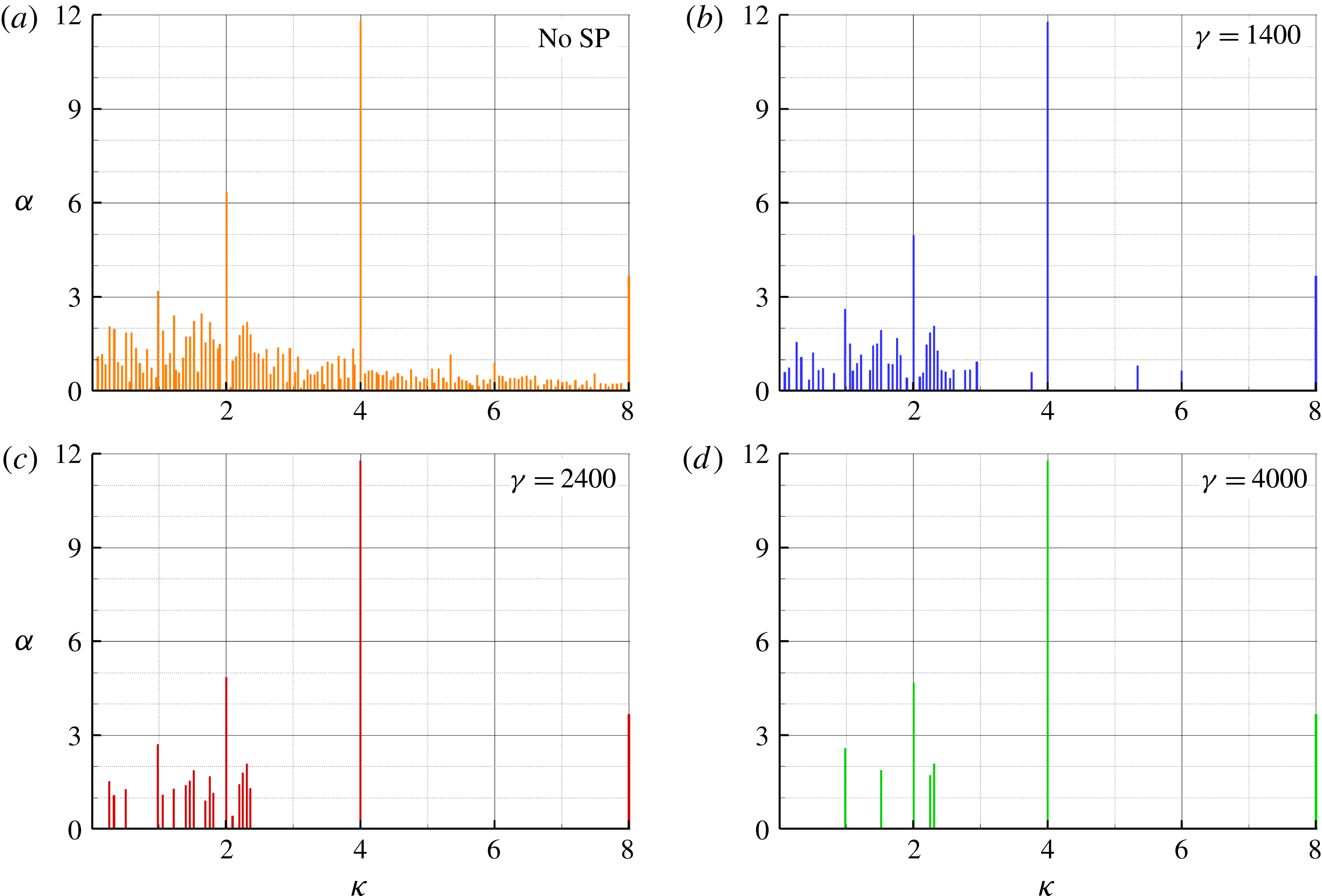
As an example, for the more loaded propeller case (
 $J=0.38$
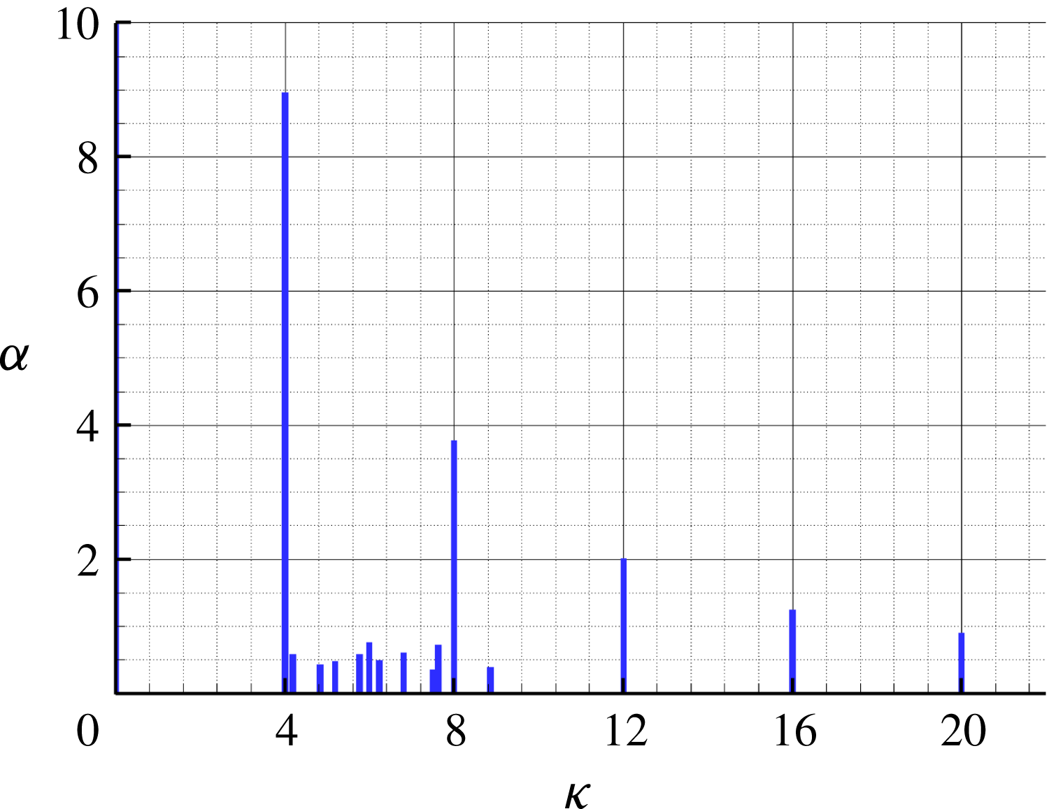
), in figure 9 the absolute value of the amplitude of the modes obtained without applying the SP algorithm is compared with the amplitude for different values of the SP parameter. In the discussion, the symbol
 $\unicode[STIX]{x1D705}$
indicates the frequency of the modes and is expressed in terms of blade passing frequency (BPF). As said above, the higher the value of
 $\unicode[STIX]{x1D6FE}$
, the smaller the number of relevant modes selected by the algorithm. However, it is possible to highlight a common trend for the different cases. In particular, starting from the almost uniform distribution of modes for
 $\unicode[STIX]{x1D6FE}=0$
, for a more selective choice of
 $\unicode[STIX]{x1D6FE}$
the spectra highlight the persistence of some dominant modes in the frequency range
 $\unicode[STIX]{x1D705}<4$
, whereas for
 $\unicode[STIX]{x1D705}>4$
only the multiples of the blade passing frequency outlive, with amplitudes that do not depend on the SP constant.
DMD spectrum for
 $J=0.38$
.

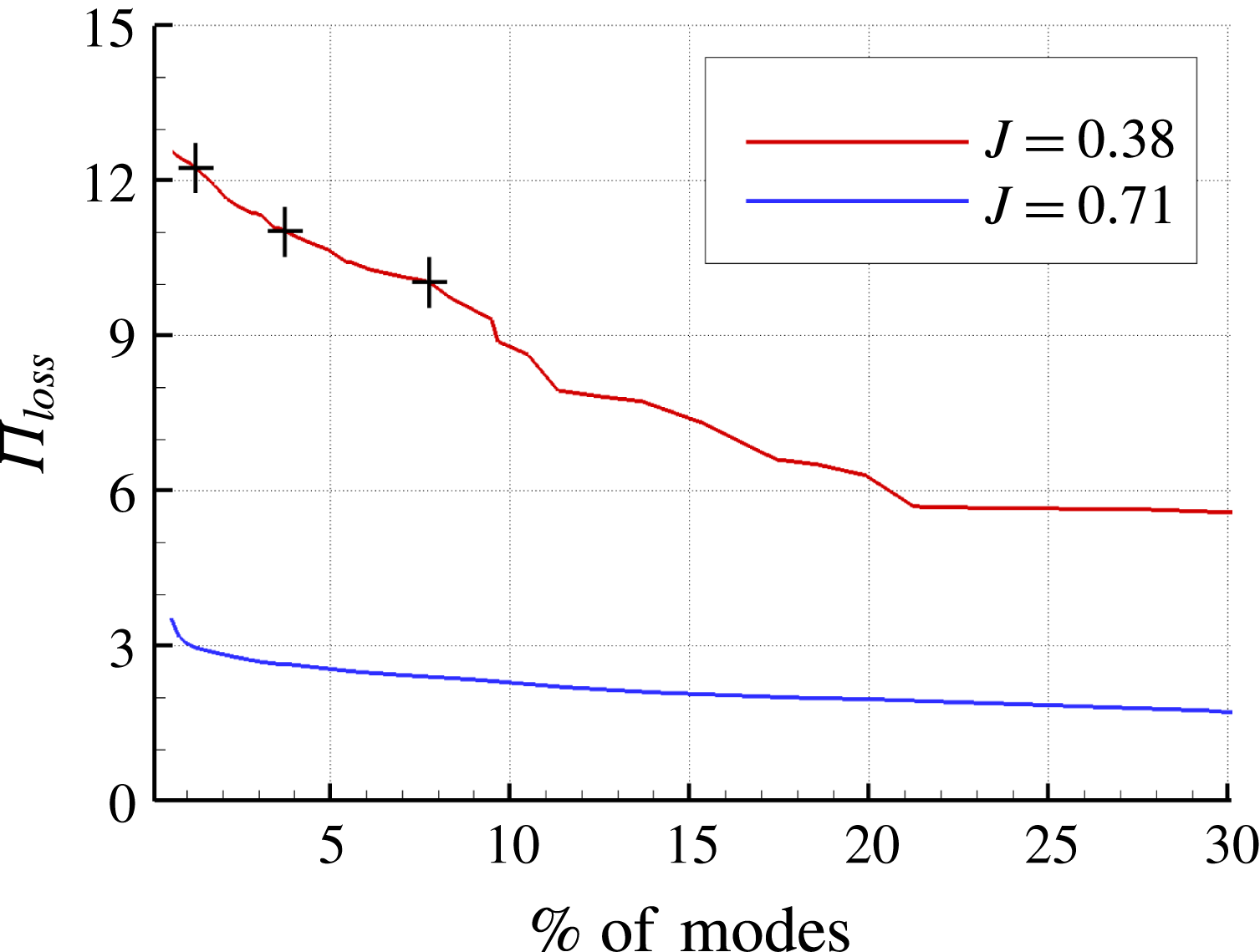
Performance loss (5.19) versus modes.

Obviously, the smaller the number of modes (i.e. the higher the value of
 $\unicode[STIX]{x1D6FE}$
) the more the quality of the least square approximation (5.17) is degraded. In figure 10 the performance loss due to the SP algorithm, defined as
 $$\begin{eqnarray}\displaystyle \unicode[STIX]{x1D6F1}_{loss}=100\sqrt{\frac{{\mathcal{J}}(\unicode[STIX]{x1D6FC})}{{\mathcal{J}}(\unicode[STIX]{x1D6FC})|_{\unicode[STIX]{x1D6FE}=0}}}, & & \displaystyle\end{eqnarray}$$
is depicted versus the per cent of non-zero amplitude modes. The symbols on the
 $J=0.38$
curve represent the three values of
 $\unicode[STIX]{x1D6FE}$
considered in figure 9. With the sole inclusion of the mean flow the performance loss is approximately 13 %, then it decreases and for
 $\unicode[STIX]{x1D6FE}=1400$
(that, in this case, corresponds to 93 modes) is 10 %. In figure 10, curve
 $J=0.71$
is also reported for comparison; it can be seen that
 $\unicode[STIX]{x1D6F1}_{loss}$
is around 3.6 % also with the mean flow alone, and weakly depends on the number of non-zero modes.
In order to remove transient modes which have high amplitudes but high decay rates, we further multiply each amplitude resulting from the SP algorithm by its damping factor
 $|\unicode[STIX]{x1D707}_{i}|^{N-1}$
(Statnikov, Meinke & Schröder Reference Statnikov, Meinke and Schröder2017). In fact, strongly damped modes influence only the early stage of time evolution. Since the aim of ROM is the identification of the most important modes for the entire available time history, the effect of these damped modes is limited and the use of their undamped amplitude can be misleading.
6 Modal analysis results and discussion
The key aspects of the wake flow qualitatively described in a previous section are synthesized and correlated to the modal decomposition provided by the POD and DMD reconstruction for the two loading conditions in the following sections.
6.1 Case
 $J=0.71$

At
 $J=0.71$
, the propeller wake keeps stable for a distance which is longer than the computational domain considered in the analysis; this is consistent with the experimental visualizations presented in Felli et al. (Reference Felli, Camussi and Di Felice2011), where the onset of instability is observed at a distance of 6–8 diameters downstream the hub. In fact, as a consequence of the moderate loading, the distance between two consecutive tip vortices is sufficiently large to delay the disruption of the blade vortex sheet with the consequent inception of the destabilization.
At this loading condition, the flow past the propeller consists of organized and ordered motion of coherent structures that preserve their morphology during the downstream convection. DMD and POD analyses correctly identify this aspect of the flow. In figure 11, the amplitude of the computed DMD modes are depicted. The spectrum of the DMD shows the dominance of frequencies that corresponds to the BPF and its multiples; a set of modes in the range between the first and the second BPF with reduced amplitudes can also be observed.
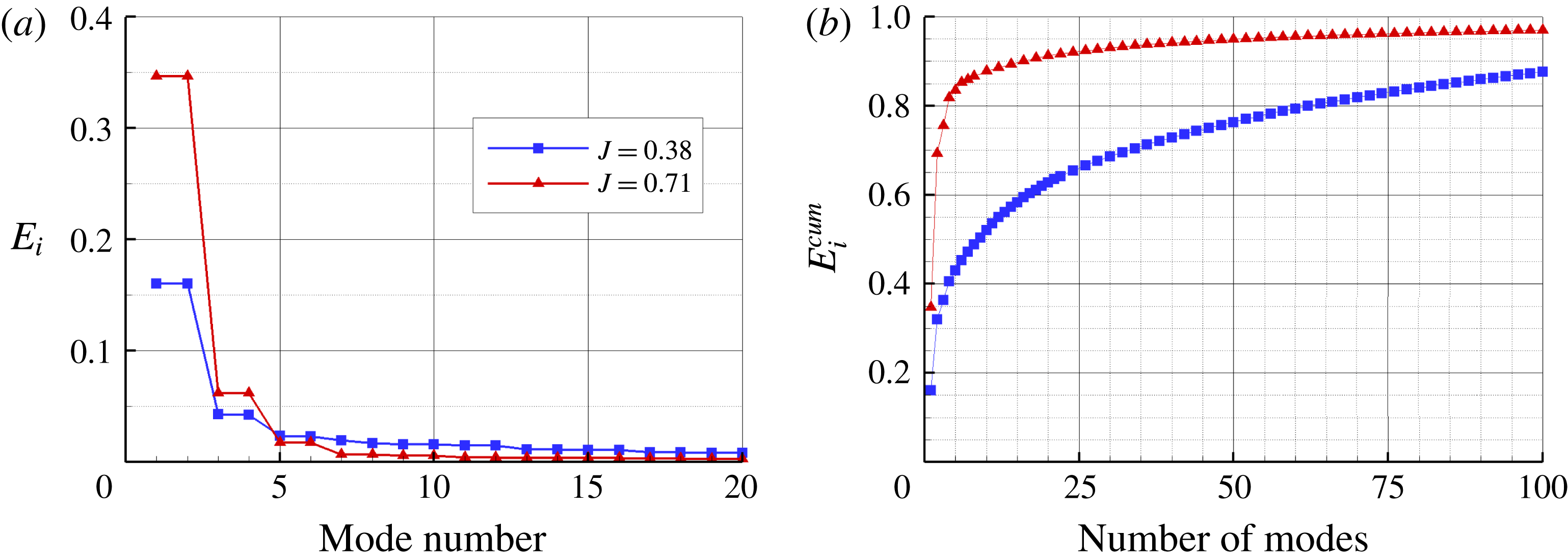
Similarly, the POD analysis confers to only a few modes the most relevant contribution to the energy content of the flow. In particular, from figure 12(b), where the cumulative energy of the POD modes is reported, it can be noted that more than 85 % of the energy of the flow has to be ascribed to the first six modes.
DMD spectrum for
 $J=0.71$
.

POD relative (a) and cumulative (b) energy of the modes.

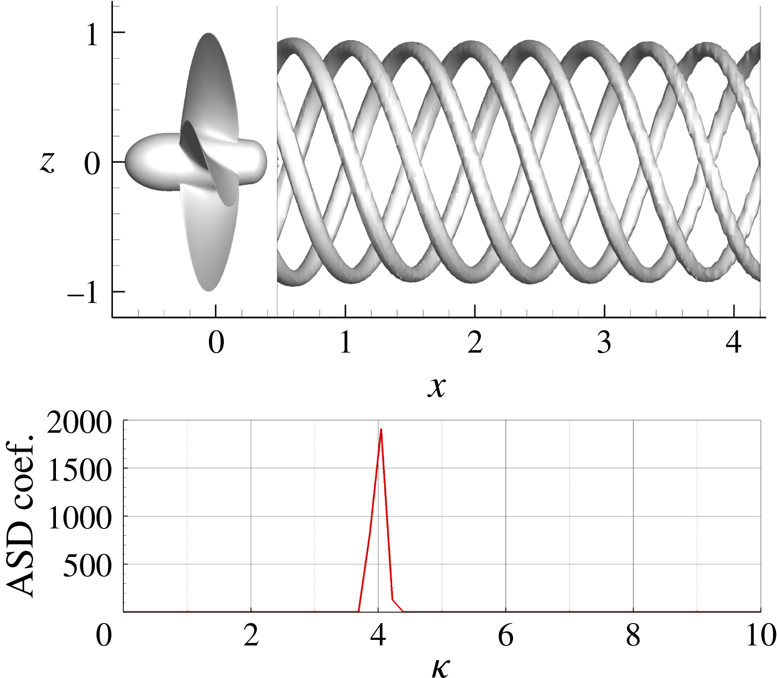
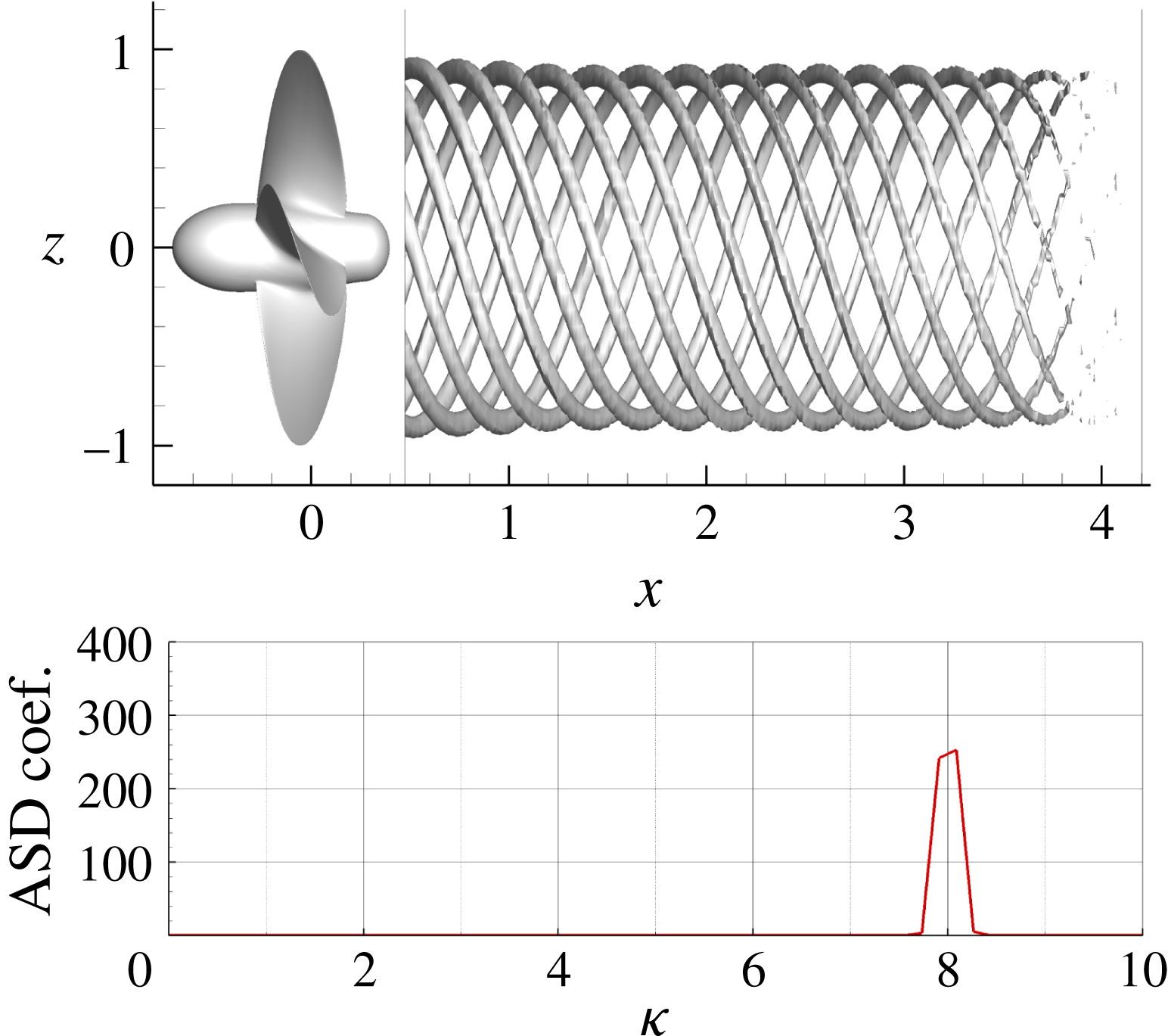
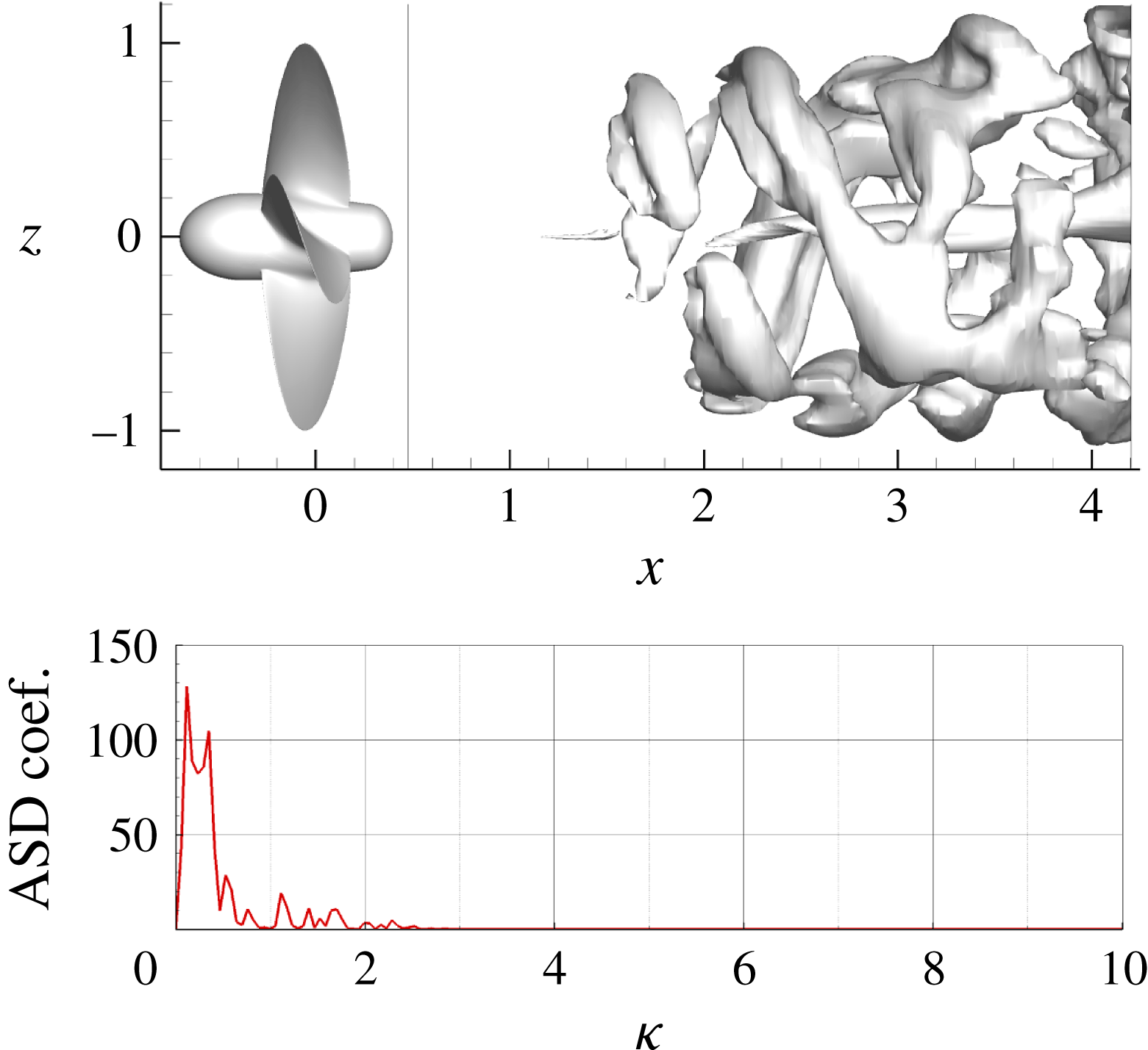
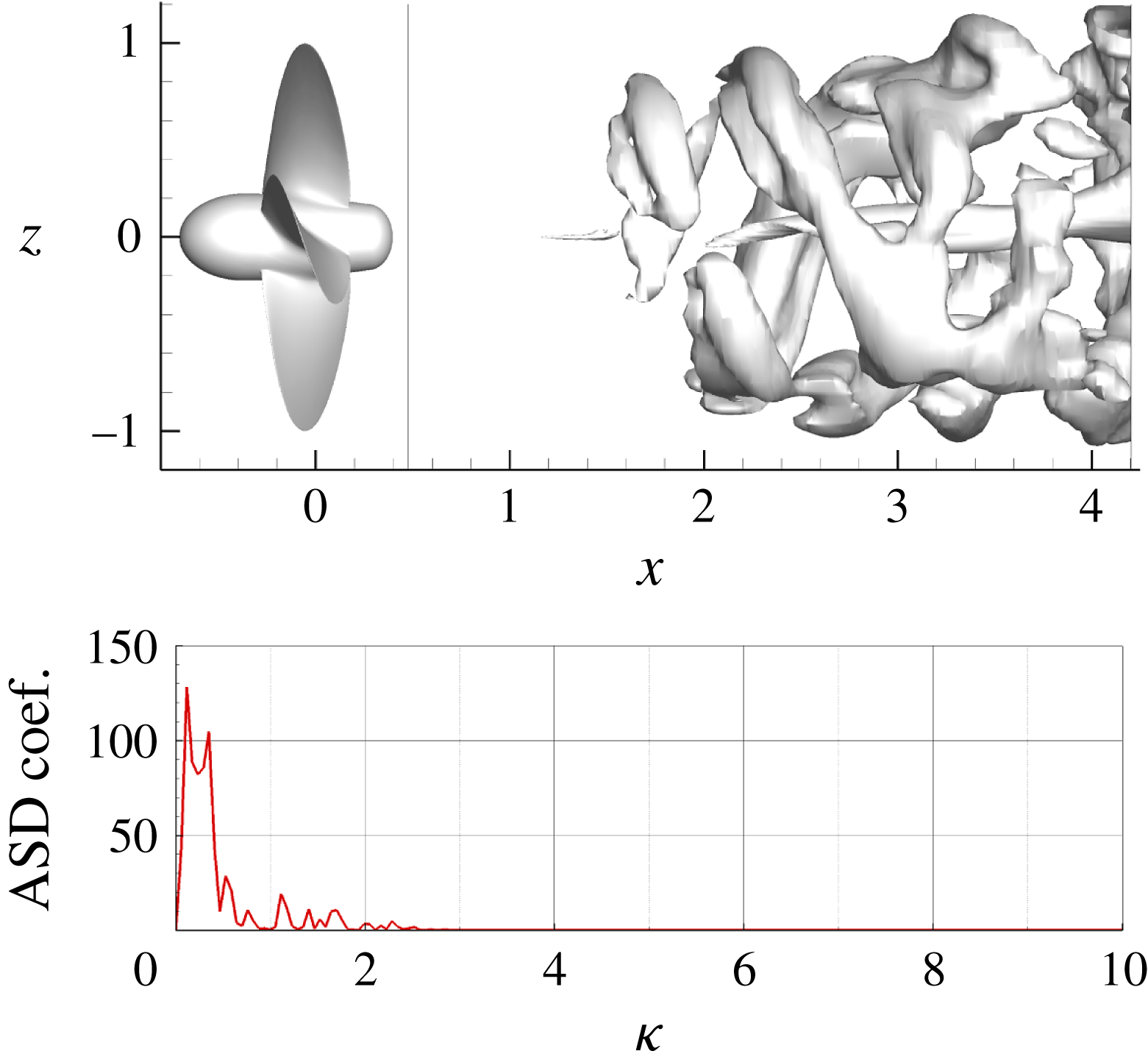
These modes of the POD decomposition identify the evolution of the coherent structures in the outer portion of the propeller slipstream and are associated with the dynamics of the tip vortices. Figures 13 and 14 show the three-dimensional representation of modes 1 and 3 in terms of constant pressure surfaces, and the correspondent auto spectral density (ASD), that is the Fourier transform of the autocorrelation function (Newland Reference Newland1993), of the temporal coefficients
 $a_{1}(t)$
and
 $a_{3}(t)$
. Clearly, the ASD associates the aforementioned modes to the first and second BPF and, consistently, the POD mode 3 is characterized by half the spatial wavelength of mode 1. Moreover, the shape of the mode is conserved for the entire length of the domain as a consequence of the stable nature of the downstream motion of the tip vortices. POD modes 5 and 7 (not shown for the sake of conciseness) are associated with the third and fourth BPF and show similar spatial features but length scales equal to
 $1/3$
and
 $1/4$
of the first mode.
DMD modes correspondent to tonal frequencies show the same spatial characteristics of the POD ones; in particular the richest dynamic content of the wake is limited to its outer portion affected by the passage of the tip vortices. For example, in figures 15 and 16 the DMD modes associated with the first and second BPF are shown; their similarity to POD mode 1 and 3, respectively, is evident.
Case
 $J=0.71$
; POD mode 1.

Case
 $J=0.71$
; POD mode 3.

Case
 $J=0.71$
; DMD mode
 $\unicode[STIX]{x1D705}=4$
.

Case
 $J=0.71$
; DMD mode
 $\unicode[STIX]{x1D705}=8$
.

As shown by Rempfer & Fasel (Reference Rempfer and Fasel1994), the POD eigenvalues occur in pairs of almost equal value. Each pair of eigenfunctions
 $\unicode[STIX]{x1D753}_{2n}$
and
 $\unicode[STIX]{x1D753}_{2n+1}$
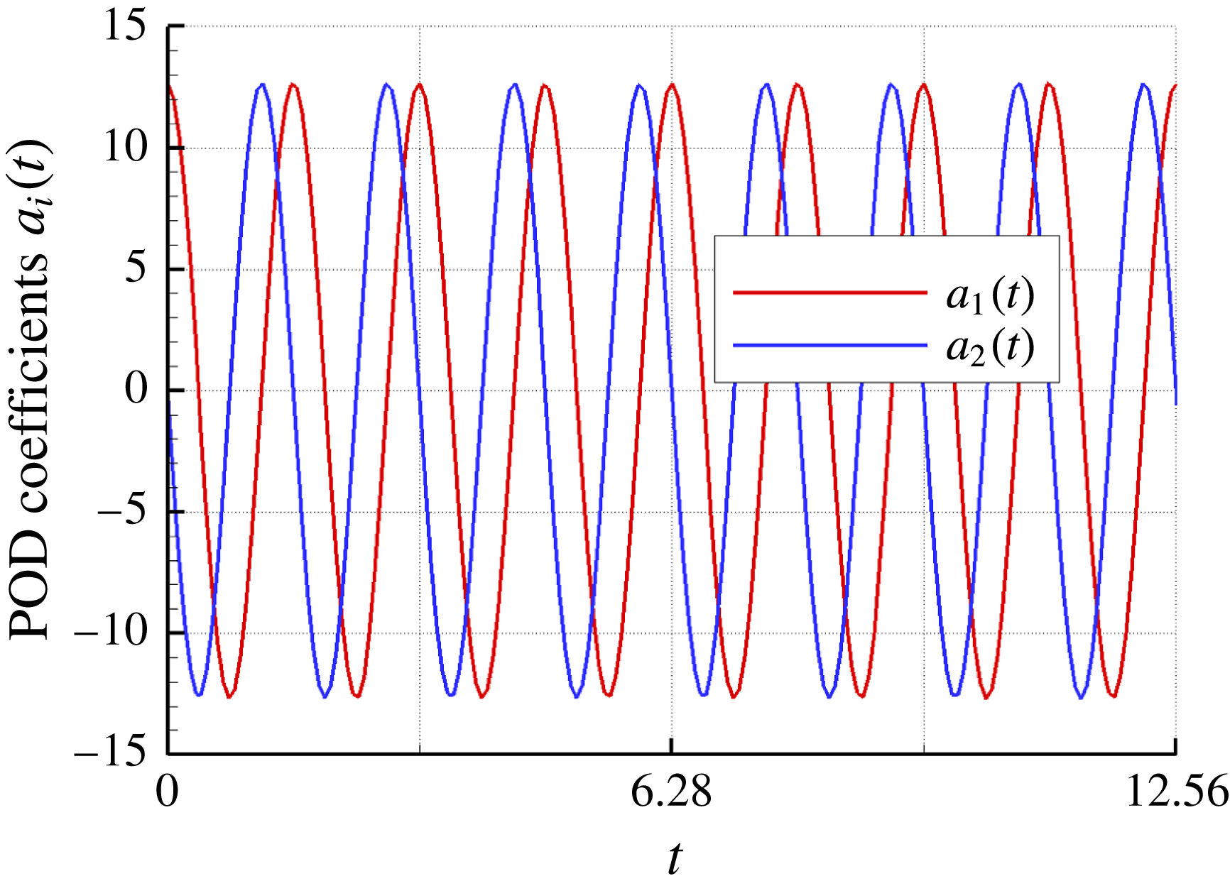
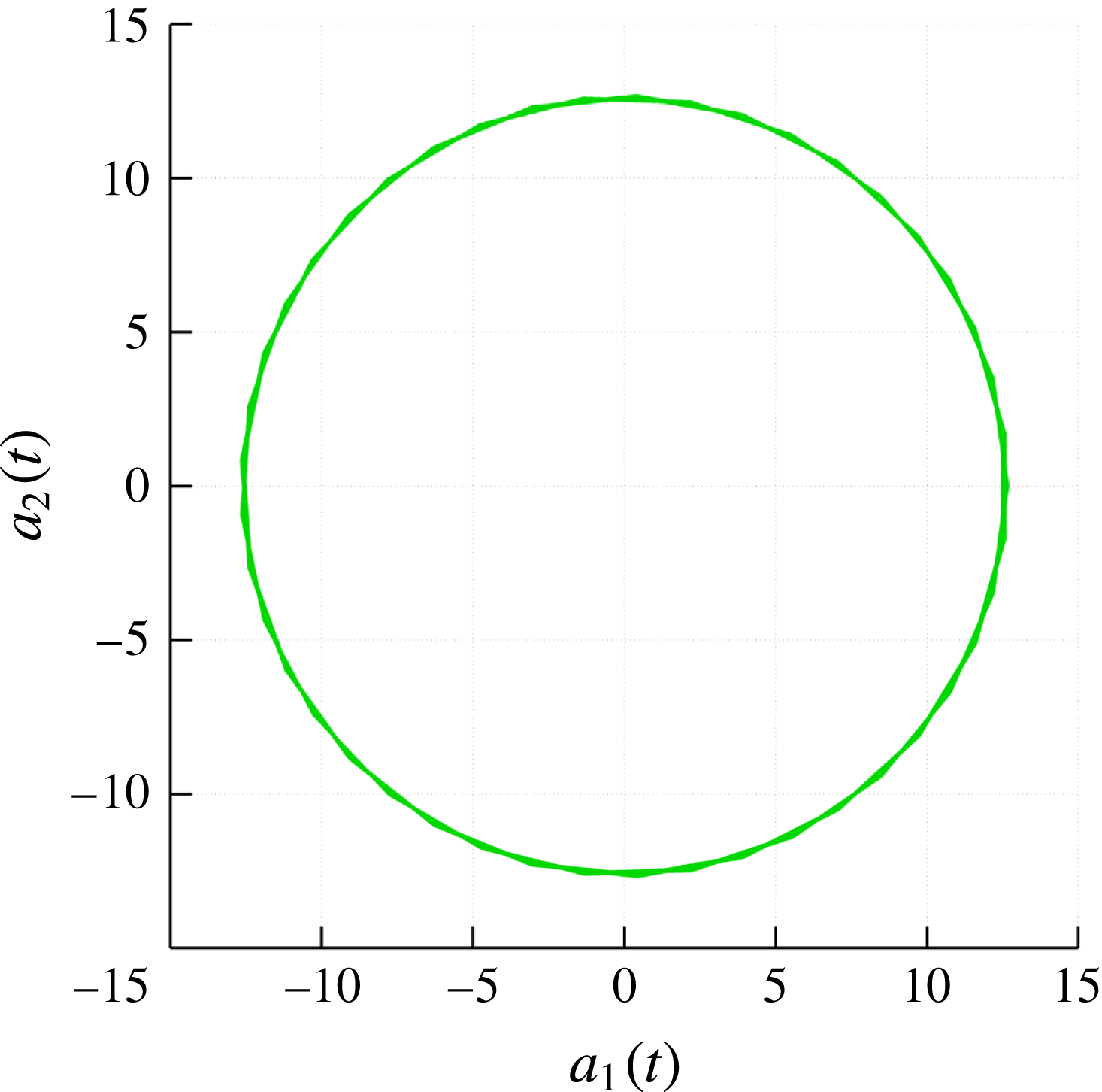
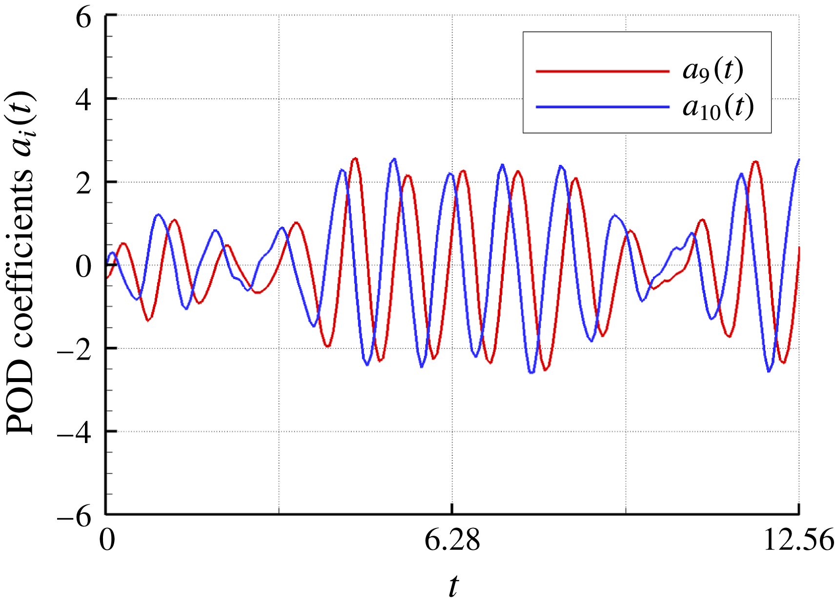
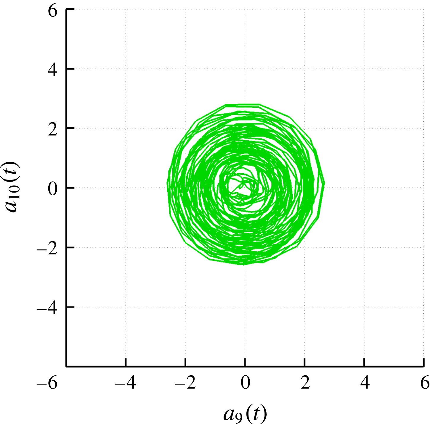
provides the shape of a related coherent structure and its evolution while moving downstream. When the coherent structure is travelling at constant speed with constant shape, the eigenvalue problem degenerates, giving rise to pairs of identical eigenvalues. This is the case of the first six POD modes, which are characterized by equal energy content, spatial distribution and spectral content of temporal coefficient in pairs. The only significant difference is a temporal shift of their related coefficients, as shown, for example, in the case of
 $a_{1}(t)$
and
 $a_{2}(t)$
in figure 17 and by the phase portrait in figure 18. In this second figure, the data describe a circle, because they represent an oscillation made of two sine waves with equal frequency but a phase shift of
 $90^{\circ }$
(Oberleithner et al.
Reference Oberleithner, Sieber, Nayeri, Paschereit, Petz, Hege, Noack and Wygnanski2011). This behaviour was already found in Sarmast et al. (Reference Sarmast, Dadfar, Mikkelsen, Schlatter, Ivanelli, Sørensen and Henningson2014) in the analysis of the flow behind a wind turbine. When the pair of eigenvalues are not exactly the same, because of the variation of the structures as they propagate, the related temporal coefficients show not only a time shift but also a small variation, as shown for example in figures 19 and 20. Moreover, in Schmid, Violato & Scarano (Reference Schmid, Violato and Scarano2012) it is shown that, for periodic and convective phenomena, a composition of a pair of (real) POD modes
 $\unicode[STIX]{x1D753}_{2n}+\text{i}\unicode[STIX]{x1D753}_{2n+1}$
coincides with a complex DMD mode, while for non-periodic or transient flows, this coincidence does not hold.
Case
 $J=0.71$
POD coefficients
 $a_{1}$
and
 $a_{2}$
.

Case
 $J=0.71$
phase portrait of coefficients
 $a_{1}$
and
 $a_{2}$
.

Case
 $J=0.71$
POD coefficients
 $a_{9}$
and
 $a_{10}$
.

Case
 $J=0.71$
phase portrait of coefficients
 $a_{9}$
and
 $a_{10}$
.

The remaining contribution to the modal description of the wake is related to flow structures that are poorly correlated to the tonal frequencies associated with the blade passage. This is evidenced by modes correspondent to non-integer frequencies, almost contiguously distributed in the frequency range between the first and second BPF in the DMD spectrum (figure 11). The amplitude of these modes is noticeably smaller than the tonal ones and, as alternatively described by the POD decomposition, provides a minimal contribution to the energetic content of the flow. In fact, modes higher than 8 contributes collectively to 15 % of the total energetic content of the flow (figure 12 b), clearly indicating that the flow is dominated by large-scale coherent motion.
The dynamic evolution of the hub region is described by POD modes starting from the ninth, with spatial and temporal characteristics comparable to those yielded by DMD. These modes consists of two systems of helical structures (figures 21–24 for the DMD and POD decomposition, respectively). Close to the hub, the modes look like a single helix with increasing pitch that, starting from the second half of the domain, evolve into a double helix with reduced pitch (i.e. reduced spatial wavelength). From the physical point of view, these modes show that in the inner region of the slipstream the perturbations are propagated by different wavelengths whose growth and decay rates overlap along the
 $x$
axis, confirming the results presented in Viola et al. (Reference Viola, Iungo, Camarri, Porté-Agel and Gallaire2014), Ashton et al. (Reference Ashton, Viola, Camarri, Gallaire and Iungo2016) for a wind turbine operating at equivalent loading condition. This aspect is supported by the presence of different frequencies in the ASD of the POD temporal coefficients
 $a_{9}(t)$
and
 $a_{11}(t)$
. Moreover, from these spectra it can be deduced that the secondary helix develops with greater strength, in particular for mode 9.
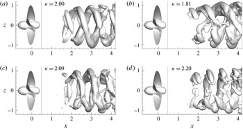
In addition to what already evidenced by the POD outcome, the DMD approach identifies a mode that describes the mutual interaction between the hub vortex and the tip vortex (figure 22). This mode is associated with
 $\unicode[STIX]{x1D705}=6.23$
(i.e. a frequency close to the average of the first and second BPF) and highlights the onset of a resonant phenomenon between the inner and the outer portions of the slipstream and the oscillatory nature of the hub vortex at frequency higher than the tonal one.
Case
 $J=0.71$
; DMD mode
 $\unicode[STIX]{x1D705}=6.23$
.

Case
 $J=0.71$
; DMD mode
 $\unicode[STIX]{x1D705}=6.00$
.

Case
 $J=0.71$
; POD mode 9.

Case
 $J=0.71$
; POD mode 11.

Case
 $J=0.71$
; correspondence of coherent structures and frequency content.

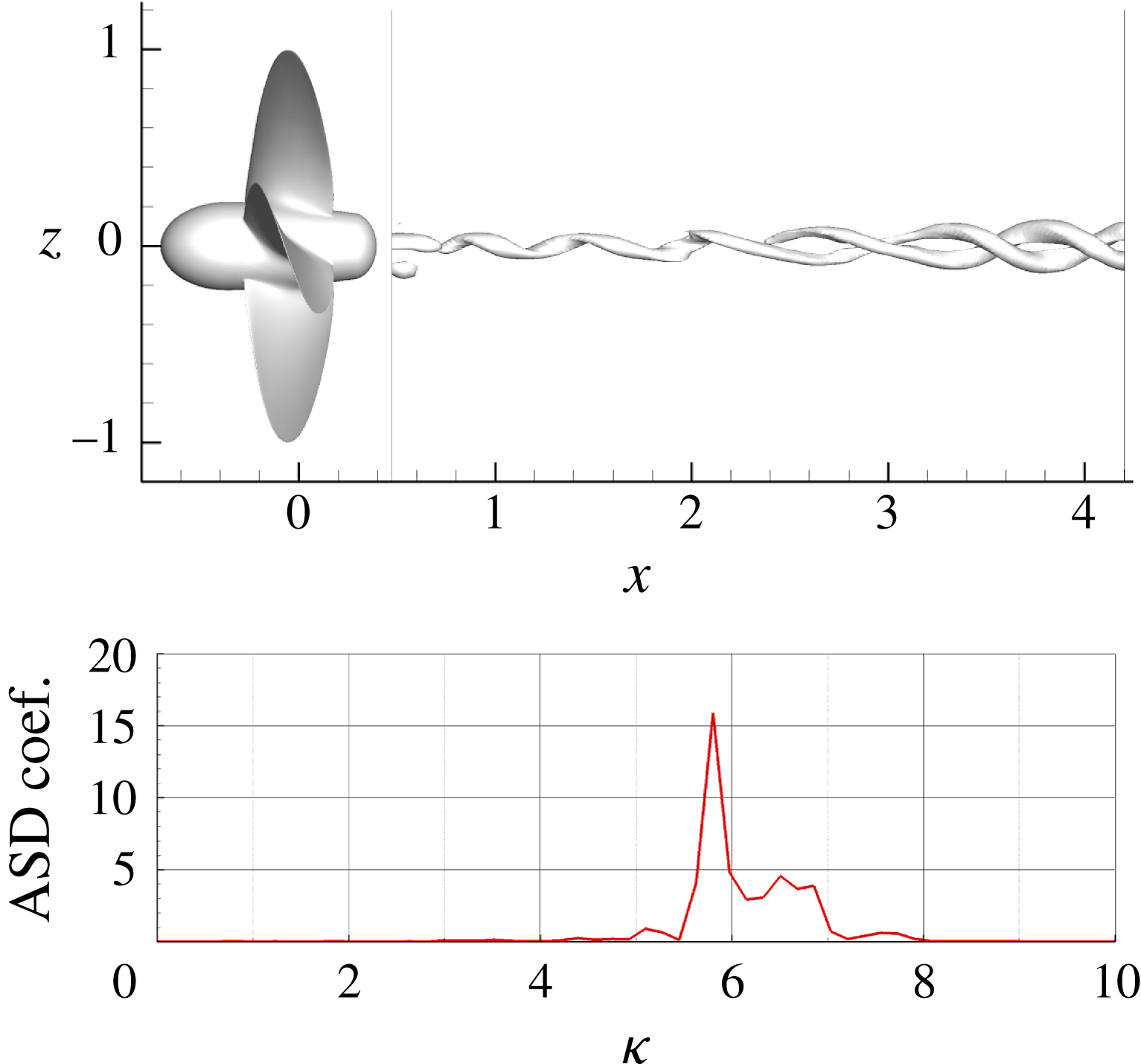
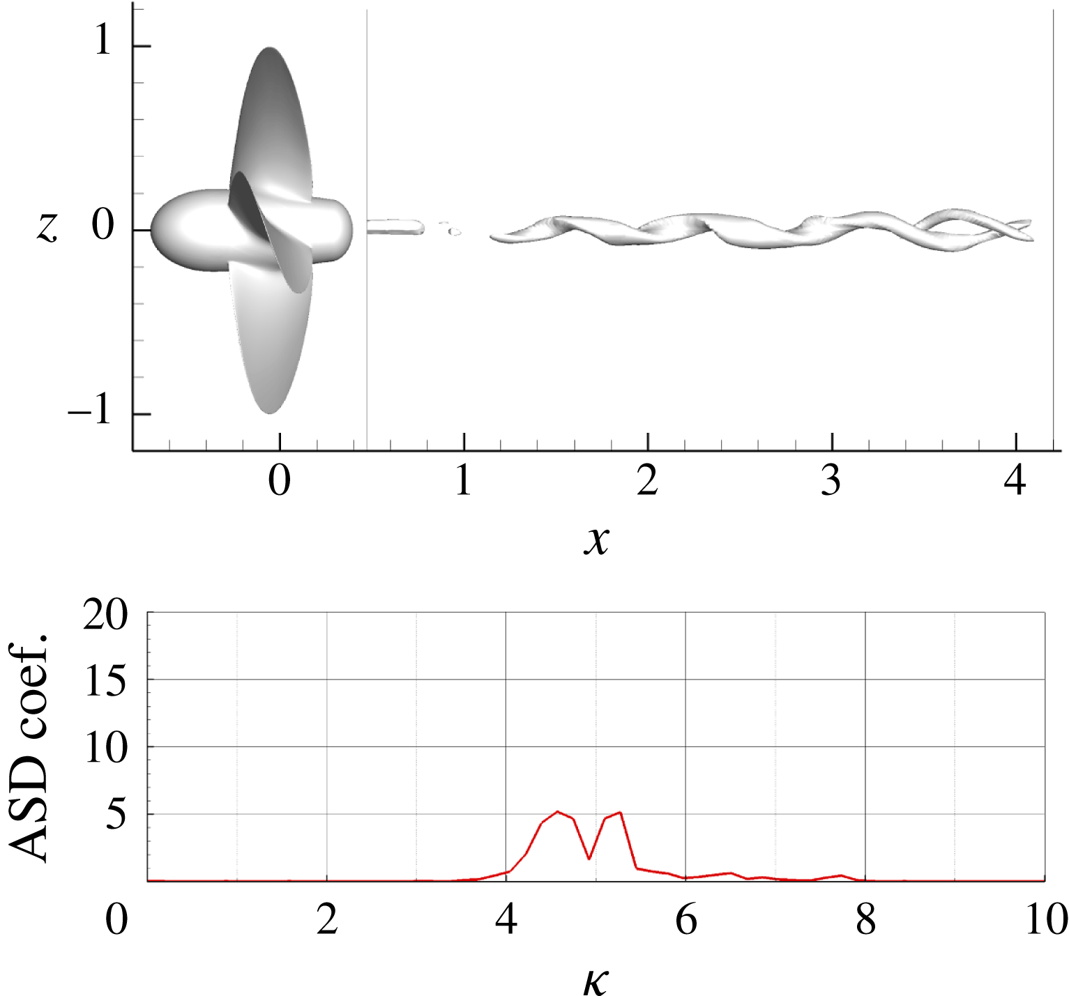
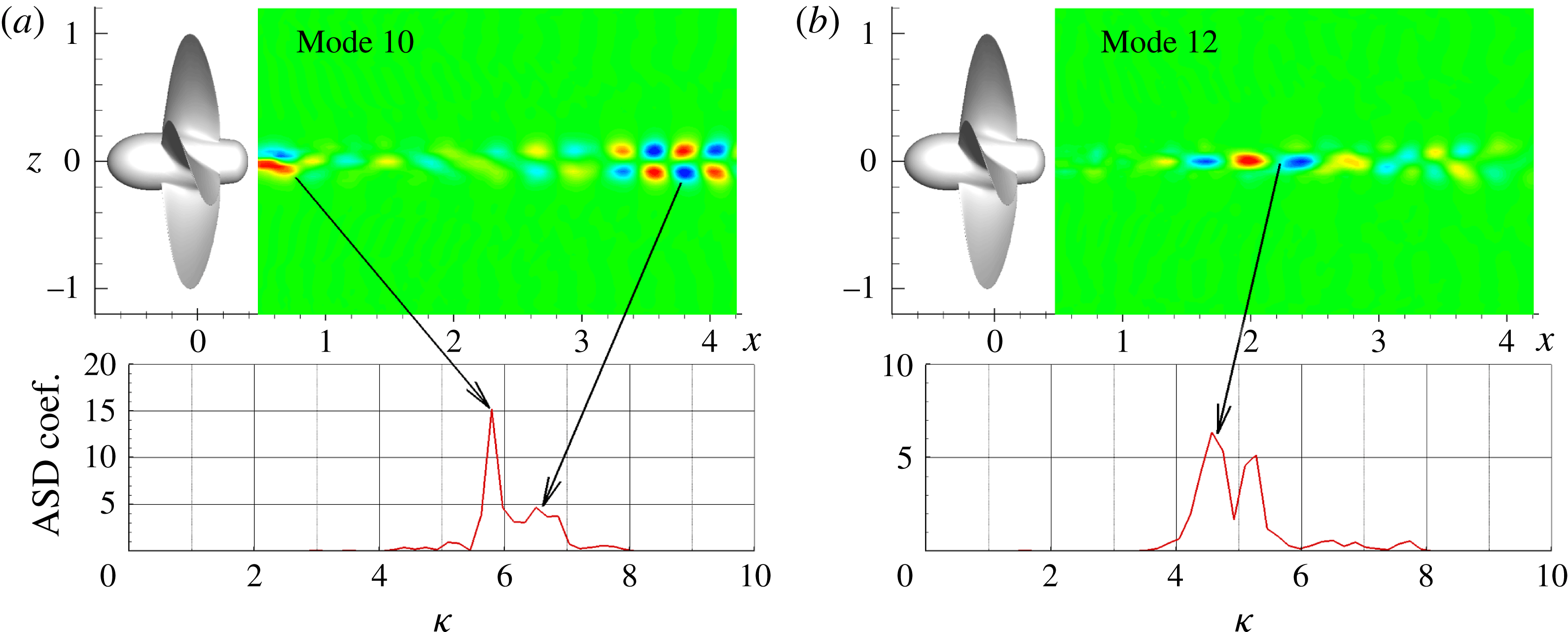
In order to inspect the multi-frequency nature of the hub vortex region, the POD analysis was also carried out for a shorter domain that excluded the region close to the propeller hub. This analysis (not entirely shown, for conciseness) permitted to associate the correct frequencies to particular structures of the modes, as shown in figure 25(a,b), that display, on a two-dimensional
 $x$
–
 $z$
section, the vertical velocity
 $w$
corresponding to mode 10 and 12. The coherent structure described by POD mode 10 is strong immediately past the propeller, because of the abrupt reduction of the hub sectional area. Slightly downstream,
 $w$
is markedly weakened for almost half of the domain and, then, reinforces with a different morphology and spatial wavelength that looks compatible with the double helix shape obtained by the three-dimensional analysis. Specifically, the peak close to
 $\unicode[STIX]{x1D705}=5.8$
can be ascribed to the perturbation close to the hub and the one close to
 $\unicode[STIX]{x1D705}=6.5$
to the fluctuations in the far field. Conversely, mode 12 in figure 25(b) evidences a different strength of the spiral: in this case, the fluctuations are stronger about the middle of the domain where the pattern resembles a single helix that gradually changes into a weaker double helix shape downstream.
The modal description, integrated by simple momentum based considerations, can give some details on the hub vortex dynamics and its relation with the flow inside the propeller slipstream. In particular, immediately past the propeller, the flow around the hub vortex is strongly perturbed due to the radial displacement of the root vortices that follow the hub surface and wrap around a region of decelerated flow around the propeller axis. These perturbations are immediately weakened by the momentum imparted by the propeller to the incoming flow and by the concurrent contraction of the propeller slipstream that further limits the radial deflections of the vortical structures. The acceleration of the flow inside the propeller slipstream is consistent with the fact that the single helix develops with an increasing pitch angle. However, as a consequence of the mild propeller loading, the length scale of the momentum gain is relatively short and, hence, the hub vortex fluctuations restart around the middle of the shown domain in a different form compatible to the double helix oscillations.
6.2 Case
$J=0.38$

At this condition, the flow complexity enriches the modal representation obtained by the POD and DMD decompositions. In particular, POD analysis highlights a significant redistribution of energy content among the modes with respect to
 $J=0.71$
, as depicted in figure 12(a). It is also interesting to notice that the cumulative energy distribution (figure 12
b) at
 $J=0.38$
is characterized by a wider spread of energy among the modes: more than 120 modes are necessary to attain 90 % of the total energy (only 16 modes are required by the more stable condition to cumulate the same amount of energy). These trends are a clear indication that, in spite of the persistence of large structures, a significant part of the kinetic energy stems from high frequency and small-scale turbulence.
The complexity of the flow condition is even better captured by the DMD, which highlights additional characteristics of the flow. The analysis of the spectrum of the SP DMD, in particular the one in figure 9(c) obtained with a high but not too selective value of
 $\unicode[STIX]{x1D6FE}$
, allows us to identify five different set of modes, of which one is related to the blade passing frequency and the others are associated with specific aspects of the destabilization mechanism, as shown by their spatial morphology. The reader is referred to the temporal sequence in figure 7 and the slipstream flow depicted in figure 8 to better follow the analysis. The five different sets of modes identified in the DMD analysis are presented and compared/integrated with the results obtain by POD.
6.2.1 Case
$\unicode[STIX]{x1D705}=4$
and multiples

This group of modes is related with the tonal frequencies, associated with the passage of tip vortices detached from the propeller blades. For these modes, the results obtained using both DMD and POD analyses are in perfect agreement. In particular, both approaches identify as the most energetic mode the first blade passing frequency
 $(\unicode[STIX]{x1D705}=4)$
. In figure 26 the pressure isosurface of the DMD mode at this frequency is depicted. Both DMD and POD analyses point out a contraction in length of the mode, when compared to the one with the same frequency in the more stable condition
 $J=0.71$
. In fact, this mode is stronger in the near wake of the propeller (up to 2.5 propeller radii) and weakens in the far field, where the wake is altered due to the destabilization (downstream the red line in figure 26).
When compared to the higher advance ratio condition, for
 $J=0.38$
the POD analysis reveals a significant loss of the energy associated with the two POD modes corresponding to
 $\unicode[STIX]{x1D705}=4$
. Indeed, their contribution to the whole energy content is around 32 % (see figure 12
a) against 70 % of the more stable condition. Also the energy associated at higher harmonic is significantly lower: 8 % and 4.6 % for
 $\unicode[STIX]{x1D705}=8$
and
 $12$
, respectively.
Case
 $J=0.38$
; DMD mode
 $\unicode[STIX]{x1D705}=4$
.

Case
 $J=0.38$
; DMD set of modes around
 $\unicode[STIX]{x1D705}=2$
.

6.2.2 Case
$\unicode[STIX]{x1D705}=2$

The modes at this frequency are associated with the pairing process of two consecutive tip vortices that occurs in the transition region of the domain, as it is evident from the inspection of figure 27(a). The visualizations by
 $\unicode[STIX]{x1D706}_{2}$
criterion (figure 6) show a very complex evolution of the tip vortices (i.e. propagation of small waves along the vortex filament, with abrupt change of pitch); all these events are partially accounted for by the modes close to the reference one at
 $\unicode[STIX]{x1D705}=2$
. In fact, their shape highlights only the perturbation of the spirals at the boundary of the slipstream, the perturbation of the hub vortex being not visible. The modes at frequency higher than 2 (figure 27
c,d) show a reduced pitch and a more evident increase of the external diameter. These modes can be associated with the global burst of the propeller slipstream occurring after the first coupling process develops (see figure 9 in Felli et al. (Reference Felli, Camussi and Di Felice2011)). The gradual increase of the sectional area stretches the vortex filaments outwards and consequently the pitch reduces; this effect is also concomitant to the averaged reduction of the speed within the propeller slipstream to satisfy mass conservation. The reference mode at
 $\unicode[STIX]{x1D705}=2$
clearly shows a spatial frequency of the tip vortices doubled with respect to the first BPF and, in particular, the pitch of the spirals is regular and azimuthally constant. On the other hand, the modes associated with neighbouring frequencies describe the displacements about this mean condition, and can be related to pairing mechanism described in the sequence of figure 7. In particular, the sequence shows that the pitch varies azimuthally for both the merged and individual structures. This variable pitch distribution is accounted for by modes at neighbouring frequencies (figure 27
b–d). All these modes recall the non-constant distribution of the pitch during a complete period of the helix but centred with respect the one at
 $\unicode[STIX]{x1D705}=2$
. The marked alteration of the pitch is obviously related to the fact that the deformation, straining and merging of the interacting vortices are localized processes.
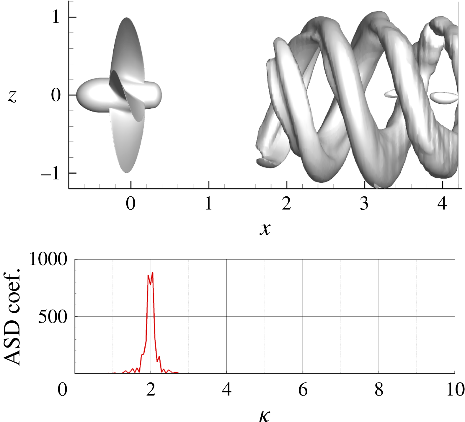
The POD analysis adds some details to the above description. In particular, modes 3 and 4 exhibit two similar peaks at 1.95 and 2.05, correlated with the pairing of adjacent tip vortices (figure 28). The energy content associated with these modes is 8 % of the total energy (figure 12 a), that is a fourth of that associated with the first two modes.
Case
 $J=0.38$
; POD mode 3.

Case
 $J=0.38$
; DMD set of modes around
 $\unicode[STIX]{x1D705}=1$
.

6.2.3 Case
$\unicode[STIX]{x1D705}=1$

This set of modes is associated with the destabilization of the hub vortex and its effects on the outer structures of the wake. These modes highlight an increasing oscillation of the hub vortex (figure 29), in accordance with the recent stability analysis for the wake of wind turbines (Ashton et al.
Reference Ashton, Viola, Camarri, Gallaire and Iungo2016). This mode is characterized by a considerably larger displacement of the outer structures of the wake (resembling the merged tip-vortex structures) with respect to the modes at
 $\unicode[STIX]{x1D705}=2$
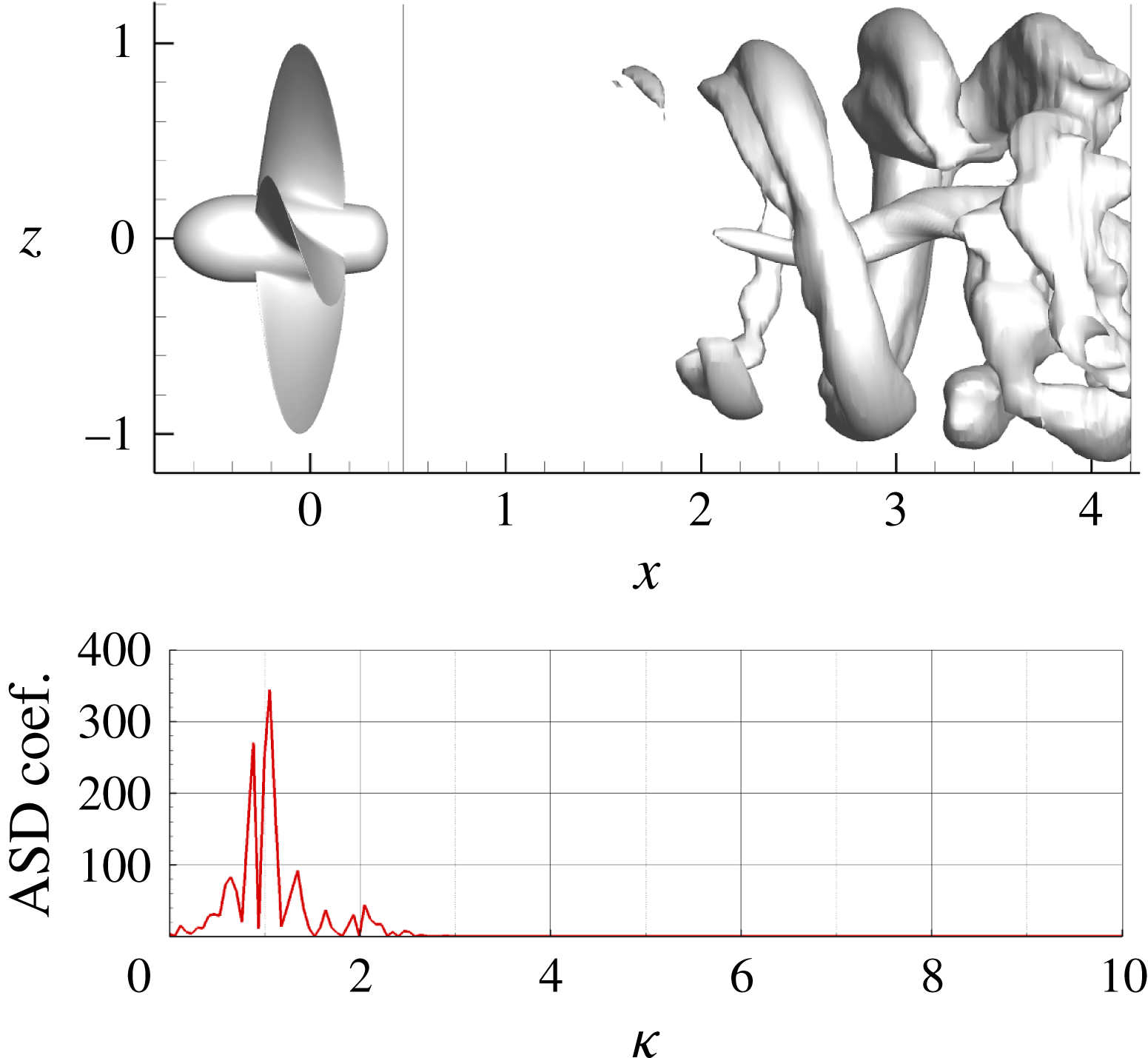
. These observations relate this mode to the precession motion of the propeller slipstream observed in the experiments by Felli et al. (Reference Felli, Camussi and Di Felice2011) and confirmed by experiments on wind turbines. The POD mode that is closer to this frequency is the seventh mode (see figure 30), which is characterized by a double peak in the coefficient spectra at
 $\unicode[STIX]{x1D705}=0.9$
and 1.05, but the associated coherent structure has a different morphology with respect to the corresponding DMD mode. This is due to the multi-component frequency spectra of the POD coefficient, as it can be evidenced also by the presence of a components at
 $\unicode[STIX]{x1D705}=1.3$
and 2.
Case
 $J=0.38$
; POD mode 7.

6.2.4 Case
$1<\unicode[STIX]{x1D705}<2$

Modes at intermediate frequencies, between the previous two last sets, can be ascribed to a sort of resonance caused by the interaction of the merged tip vortex system with the hub vortex. The information synthesized by these modes allows us to gain a deeper insight on the propagation of the destabilization from the outer to the inner structures of the propeller slipstream.
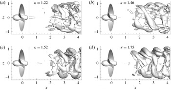
The morphology of these modes changes remarkably with the frequency (figure 31). Modes close to
 $\unicode[STIX]{x1D705}=1$
(e.g.
 $\unicode[STIX]{x1D705}=1.22$
) are characterized by external structures with small pitch, resembling vortex rings, and a strong fluctuating structure in the hub region. With the increase of
 $\unicode[STIX]{x1D705}$
, the central structure progressively weakens and the external ones exhibit strong variations of the pitch along the azimuthal position. This latter characteristic underlines the deformation and the straining of the tip structures already observed for the modes at
 $\unicode[STIX]{x1D705}=2$
and associated with their interaction and pairing.
These modes confirm what suggested by both numerical and experimental visualizations, namely that the core of the slipstream starts to oscillate after the destabilization of the outer region. In fact, as the pairing process starts, the circumferential variation of the pitch of outer filament causes the unbalance of the induced velocities to the hub vortex and hence promotes its destabilization. At first, this mechanism slowly builds up and the fluctuations of the hub become non-negligible downstream of tip vortices pairing, as shown by the systematic analysis provided in Felli et al. (Reference Felli, Camussi and Di Felice2011), figure 10. This delay can be ascribed to the stabilizing effect exerted by the acceleration within the propeller slipstream and its consequent contraction. Due to the higher loading, this effect is stronger than for
 $J=0.71$
. This inertial effect persists for a longer period, because, when the tip vortices merge, the hub vortex evolve as an independent structure, the blade vortex sheet being cut (Felli & Di Felice Reference Felli and Di Felice2005; Felli et al.
Reference Felli, Camussi and Di Felice2011); on the contrary, the outer region results more prone to destabilization because of the shear effect caused by the contact with the undisturbed, slower flow.
On the basis of the above description, the mode at
 $\unicode[STIX]{x1D705}=1.46$
can be associated with the mutual and self-sustained excitation between the merged tip vortices and the hub vortex. These interactions lead to the physical behaviour described at lower frequencies: the oscillation induced on the outer structure amplifies the shear at the boundaries of the propeller slipstream that, in its turn, dampens out the hub vortex oscillation and frequency.
Interestingly, the modes closer to the resonant frequency are the most important ones, as it can be deduced by the disappearing of modes at frequencies at the extremities of the interval (see spectra for
 $\unicode[STIX]{x1D6FE}=2400$
). Moreover, the modes that excite the hub vortex are those that show a non-constant pitch in the azimuthal direction, that cause an unbalanced perturbation to the inner vortex structure. Approaching the frequency of the second BPF, the shape of the correspondent modes reveals the progressive weakening of the hub vortex.
Case
 $J=0.38$
; DMD modes with frequencies between
 $\unicode[STIX]{x1D705}=1$
and
 $\unicode[STIX]{x1D705}=2$
.

6.2.5 Case
$\unicode[STIX]{x1D705}<1$

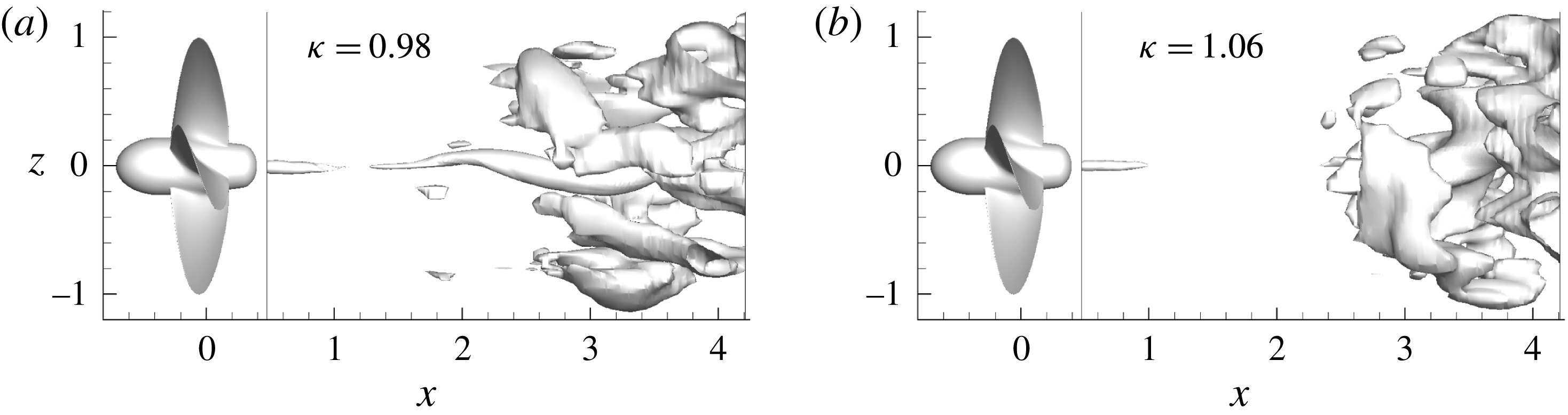
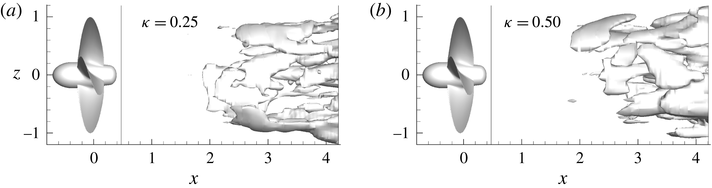
Modes at frequencies lower than 1 appear in the DMD analysis only for moderate values of
 $\unicode[STIX]{x1D6FE}$
, and also in the POD but with a very small energy content. Representative modes of this group are shown in figure 32(a,b); their features suggest their connection with the precession motion of the slipstream considered as a vortex tube. In particular, in the outer region of the slipstream, the tip vortices are not distinguishable; instead, a homogeneous sheet generated by the shear forces (arising from the contact with the external flow) can be observed. The shear, on its turn, dampens the precession motion excited by the hub vortex. The POD analysis (figure 33) allows us to capture this particular feature of the flow, and provides also an information concerning the associated energy, which is quite small (0.7 %). Moreover, it can be observed that the perturbation of the hub vortex is visible only at the end of the domain, further downstream with respect to modes related to hub vortex excitation by the tip vortex system (i.e.
 $1<\unicode[STIX]{x1D705}<2$
).
Case
 $J=0.38$
; DMD modes with frequencies
 $\unicode[STIX]{x1D705}<1$
.

Case
 $J=0.38$
; POD mode 21.
6.3 Further comments on the hub vortex dynamics
It is interesting to note the different shape of the modes associated with the dynamics of the hub vortex between the two loading conditions. At
 $J=0.71$
the modes of the hub vortex show a transition from a single helix close to the propeller to a double helix close to the end of the domain. On the other hand, at
 $J=0.38$
the modes are shaped like a single helix in the inner region (and someway coupled with the outer region of the slipstream). This difference can be explained by considering the relation between the advance coefficient (propeller loading) and the geometry (pitch angle) of the vortex structures shed by the blades, in addition to the comments on the momentum/energy transfer imparted by the propeller discussed above. Specifically, the pitch angle is strictly related to the three-dimensional features of the induced velocity field within the slipstream. For example, during very high loading conditions the wake structures resemble vortex rings and the induced velocity has a dominant axial component; conversely, as the propeller loading is gradually reduced, the helix elongates and the tangential component increases. At
 $J=0.71$
, the oscillations of the hub vortex are not damped, because of the weak acceleration of the flow; moreover, they can be amplified by a non-negligible tangential velocity induced by the vortex structures in the outer region of the slipstream. On the contrary, at
 $J=0.38$
, the momentum transfer is remarkably stronger in the wake and no evidence of such a transition is visible in the inner region, the prevailing disturbance being caused by the coupling process of the tip vortices.
7 Some remarks on the application of POD and DMD to marine propeller flows
From the above discussion, it can be concluded that POD and DMD provide similar results, in terms of mode shape, amplitudes and characteristic frequency, in zones of the domain where the evolution of the flow is driven by an almost deterministic forcing (the tip vortices in the near field, figures 13 and 15, the merged tip vortices in the far field for the highest loading condition, figures 27(a) and 28); conversely, the differences are evident where the different vortical systems of the wake interact with each other (far from the propeller plane).
However, the insight provided by both techniques is very useful for the development of reduced-order models of propeller wakes to be used as fast fluid dynamics solver within optimization algorithms. In fact, current trends in ship design (e.g. Grigoropoulos et al. Reference Grigoropoulos, Campana, Diez, Serani, Goren, Sarioz, Danisman, Visonneau, Queutey and Abdel-Maksoud2017) requires the inclusion of realistic operative scenarios, and therefore the availability of simplified and accurate models is crucial to get accurate prediction.
At the same time, the modal analysis of the wake for a marine propeller can be used to gain more insight on specific aspects still not completely understood (like noise generation and propagation). For instance, for non-cavitating conditions, the hydroacoustic performance of a marine propeller is strongly related to the turbulent wake (quadrupole component, Ianniello, Muscari & Di Mascio (Reference Ianniello, Muscari and Di Mascio2013), Ianniello (Reference Ianniello2016)) and the comprehension of the relation between these sources and the near/far acoustic noise is fundamental to develop direct or indirect control of the phenomenon. In this regard, the specific application of a decomposition technique to these problems deserve a brief comment. In literature exist many variants of the POD and DMD algorithms that are almost equivalently applied to optimization or control problems, such that a neat demarcation between the scope of these two approaches does not exist. When considering the specific algorithms presented in the present work, SP DMD seems to be preferable with respect to POD for hydroacoustic problems, because the sound radiated by turbulence amounts to a minimal fraction of the energy of the flow (Freund & Colonius Reference Freund and Colonius2009). On the other side, both methods similarly reproduce modes related to characteristics frequencies of the process, required to describe both tonal noise and loading on the rudder and the hull.
However, it should be noted that, from the computational point of view, SP DMD is more demanding with respect to POD, in terms of both memory and CPU time (mainly because of the optimization problem). The impact of this aspect on the analysis greatly depends on computational resources. In our specific case, as already said, both the size of the interpolation mesh (used for the analysis) and the number of processed snapshots were dictated by the feasibility of the DMD.
8 Conclusions
In the present paper, we used modal analysis based on proper orthogonal decomposition and dynamic mode decomposition to study the flow in the wake of a marine propeller.
The aim of the proposed analysis was to relate the output of the two modal representations with the flow physics and, moreover, to compare effectiveness of the two approaches in identifying the underlying temporal and spatial scales of the flow.
In general, the wake of a rotor (consisting of tip vortices, hub vortex and the blade vortex sheets that link the two vortical systems) is initially stable. During the downstream convection, the mutual interaction among the vortex structures and the viscous dissipation alter the original morphology. This process can be amplified by destabilization mechanisms that depends on the actual operating condition (loading) of the device.
In general, the identification of spatial and temporal scales of this process is a challenging task because the onset of instabilities introduces temporal and spatial scales that differ from the tonal ones (related to the geometric properties of the rotor, like number of blades). In the present paper, this kind of analysis was carried out for the wake field past the INSEAN E779A four bladed propeller; the flow field was obtained by detached eddy simulation for open water tests in axial inflow with two different advance coefficients, representative of light and high propeller loading conditions. The two operating speeds give rise to completely different wakes. At the highest advance ratio the vortex system is stable, whereas in the other case the destabilization of the flow is pronounced. As a result, the modal decomposition for the two flows is deeply different and helps correlate the spatial shape of the modes and the characteristics frequencies with the underlying physics.
The most interesting case investigated was undoubtedly the highest loading condition (lower advance ratio
 $J=0.38$
), it being characterized by an abrupt onset of destabilization and vortex interaction phenomena. In this case, the tonal modes (first BPF and its first multiple) are prevalent only close to the propeller, where the flow is stable. In the transition region these modes die out and different spatial and time scales appear. In particular, the destabilization of the wake is originated by the coupling of consecutive tip vortices that induce a global fluctuation and deformation of the propeller slipstream. In this region, both POD and DMD analyses converged in the identification of modes characterized by time scales and spatial wavelength greater than the tonal ones and describing processes related both to the coupling between the tip vortices and to the hub vortex dynamics. In particular, the identified modes around
 $\unicode[STIX]{x1D705}=2$
describe the pairing process of the tip vortices and the consequent distortion, stretching and localized alteration of single vortex filaments.
Modes at frequency in the range
 $1<\unicode[STIX]{x1D705}<2$
identify the interaction between the hub vortex and the novel vortex system formed by the merging of tip vortices. These modes can be associated with a mutual excitation of the two systems: the coupling of the tip vortices perturbs the hub vortex due to abrupt change of the induced velocity field and, in turn, the fluctuations of the hub vortex impose a meandering motion to the wake that superposes to the dynamics of the outer structures. Finally, modes at frequencies equal to and lower than
 $\unicode[STIX]{x1D705}=1$
are mainly associated with the precession mechanism driven by the hub vortex and are the cause of increase in fluctuations of the slipstream in the far wake. The spatial features of these modes differ from those of the previous groups, because the periodicity of the outer structures is lost, and their dominant feature is the viscous shear at the slipstream boundary; moreover, this shear acts to damp the precession motion.
In case of
 $J=0.71$
, the flow dynamics is mainly associated with the stable and ordered convection of the tip vortices, because of the weaker interaction among the vortical structures. In fact, the dominant modes identified by both techniques are characterized by spatial wavelengths and frequencies related to multiples of the BPF along the whole computational domain. Similarly to the previous case, the dynamics of the hub vortex is characterized by the competition of modes with a frequency between the first and the second BPF. Nevertheless, although the hub vortex is more stable than in the case
 $J=0.38$
(at least in the computed domain), the modes associated with the hub vortex exhibit an interesting transition from single helix close to the propeller to double helix farther downstream. Energetic and kinematic considerations related to the propeller loading suggest that this transition is associated with the fact that the fluctuations of the hub vortex, caused by the interaction of root vortices, are not sufficiently quenched by the mild accelerating action of the propeller. It is worth noting that the DMD identifies a mode (approximately at
 $\unicode[STIX]{x1D705}=6$
) that describes the coupling of the tip vortex system and the hub vortex in correspondence of the transition from single to double helix.
Finally, it must be observed that standard DMD, contrarily to the POD, does not provide a hierarchy of modes, and the selection of the most representative ones is not trivial. With respect to similar analysis on rotor flows, in the present research a Sparsity Promoting version of the DMD algorithm was successfully considered, due to its objective capability in identifying the most representative subset of modes.
Acknowledgements
We acknowledge the CINECA award under the ISCRA initiative, for the availability of high performance computing resources and support, necessary for the numerical simulations that yielded the post-processed datasets. For the DMD analysis, we used the sparsity promoting DMD functions developed by Dr Jovanović, downloadable from http://www.umn.edu/∼mihailo/software/dmdsp/.