1 Introduction
Interplay of hydrodynamic and magnetic instabilities is ubiquitous in various astrophysical, geophysical and engineering flows. Theoreticians have long used various simple background model flows to find fundamental mechanisms of such interplay. Studies based on the magnetohydrodynamic (MHD) framework revealed that the character of the instability depends on the typical Alfvén wave speed of the magnetic field; if it is faster/slower than the typical fluid flow speed, the flow is called super-/sub-Alfvénic.
In the simplest case, the background velocity
 $\boldsymbol{V}_{b}$
is assumed to be proportional to the Alfvén velocity of the background magnetic field
 $\boldsymbol{B}_{b}$
:
 $$\begin{eqnarray}\boldsymbol{B}_{b}=B_{0}\boldsymbol{V}_{b}.\end{eqnarray}$$
Here the constant
 $B_{0}$
is the inverse of the magnetic Mach number. Tataronis & Mond (Reference Tataronis and Mond1987) used (1.1) and revealed the existence of an ideal instability for sub-Alfvénic flows
 $|B_{0}|>1$
for cylindrical screw pinch plasmas. The flow (1.1) is also relevant for the competition of the Kelvin–Helmholtz and tearing instabilities, both of which occur when the base field has an inflection point. As discussed in Chen, Otto & Lee (Reference Chen, Otto and Lee1997), the Kelvin–Helmholtz/tearing mode appears only when the flow is sub-/super-Alfvénic; the stabilisation of the Kelvin–Helmholtz/tearing mode by a magnetic field/shear has also been observed in various flow configurations; see Chandrasekhar (Reference Chandrasekhar1961), Miura & Pritchett (Reference Miura and Pritchett1982), Einaudi & Rubini (Reference Einaudi and Rubini1986) and Ofman, Morrison & Steinolfson (Reference Ofman, Morrison and Steinolfson1993). All those ideal (i.e. diffusionless) modes are stabilised when approaching
 $|B_{0}|=1$
, consistent with the theorem derived in Chandrasekhar (Reference Chandrasekhar1956). The theorem claims that the flow (1.1) with
 $|B_{0}|=1$
is stable when the following three assumptions are satisfied.
(i) The nonlinearity of the perturbation is negligible.
(ii) The flow is ideal, i.e. no diffusion.
(iii) The magnetic field perturbation is negligibly small on the flow boundary.
The last assumption can be replaced by the perfectly conducting conditions on the boundary (Chandrasekhar Reference Chandrasekhar1961).
There has been a great deal of research on the linear analyses of various MHD instabilities, and the subsequent nonlinear developments of the growing perturbations. However, the linear analysis is formally only valid for infinitesimally small perturbations, and thus the transition to turbulence may occur by large perturbations even when the laminar state is linearly stable. In fact, when an inviscidly stable shear predominantly drives the flow, the most dangerous route to turbulence is typically caused by three-dimensional finite-amplitude perturbations (e.g. Schmid & Henningson Reference Schmid and Henningson2001). In hydrodynamic shear flow studies, the finite-amplitude instability that is responsible for such bypass transition route is widely referred to as ‘subcritical instability’, because the transition occurs at smaller Reynolds number than the critical value determined by the linear stability analysis.
Subcritical instabilities in MHD flows have by comparison received little attention. The aim of this paper is to theoretically and numerically analyse such subcritical MHD instabilities in broad sub- and super-Alfvéneic regimes. We select the magnetised plane Couette flow under the condition (1.1) as a model profile. This flow is among the fundamental problems in classical fluid dynamics, and has long served as an archetypal model in the study of subcritical instability. The laminar base flow induced by the movement of the walls is merely a homogeneous shear, and the magnetic field has the same structure when a uniform current exists within the walls. This means that the laminar flow is designed to be free from any of the inviscid hydrodynamic and ideal MHD instabilities mentioned above. Moreover, it is not too difficult to numerically confirm that there is no linear instability found in this flow using the linearised viscous–resistive MHD equations. Therefore, transition to turbulence in the flow must always occur by the subcritical instability mechanism.
This study is motivated by a number of dynamical systems theory studies of purely hydrodynamic shear flows. In the phase space, the subcritical transition problem boils down to the analysis of the hyper-surface that separates the regions of laminar and turbulent attraction. The key finding in this approach to the study of shear flow is that there are special finite-amplitude invariant solutions (e.g. steady states, travelling waves, periodic orbits) that are ultimately responsible for transition to turbulence (Itano & Toh Reference Itano and Toh2001; Skufca, Yorke & Eckhardt Reference Skufca, Yorke and Eckhardt2006). For the plane Couette flow, Wang, Gibson & Waleffe (Reference Wang, Gibson and Waleffe2007) showed that the stable structure on the hyper-surface is the steady solution found in Nagata (Reference Nagata1990) and Clever & Busse (Reference Clever and Busse1992), hereafter called the NBC solution. Subsequently, the result of Wang et al. (Reference Wang, Gibson and Waleffe2007) is found to be consistent with the large-Reynolds-number asymptotic analysis by Hall & Sherwin (Reference Hall and Sherwin2010) and Deguchi & Hall (Reference Deguchi and Hall2016), extending the vortex–wave interaction theory of Hall & Smith (Reference Hall and Smith1991) developed for boundary-layer flows. The strong link between the finite-amplitude invariant solutions and the subcritical transition to turbulence has also been reinforced by the pipe flow experiments of Hof et al. (Reference Hof, van Doorne, Westerweel, Nieuwstadt, Faisst, Eckhardt, Wedin, Kerswell and Waleffe2004) and De Lozar et al. (Reference De Lozar, Melibovsky, Avila and Hof2012). In MHD shear flows under Kepler rotation, the importance of the subcritical instability has been pointed out repeatedly, for example by Rincon, Ogilvie & Proctor (Reference Rincon, Ogilvie and Proctor2007) and Riols et al. (Reference Riols, Rincon, Cossu, Lesur, Longaretti, Ogilvie and Herault2013). The invariant solutions in the non-rotating MHD plane Couette flow have been studied only recently in Deguchi (Reference Deguchi2019a ,Reference Deguchi b ), together with their large-Reynolds-number asymptotic development. The present work will extend that result for broader magnetic Mach numbers.
The profile (1.1) is experimentally realised in magnetised Taylor–Couette flow, which has been much studied in the past three decades as a simple model of astrophysical rotating flows (see the review article by Rüdiger et al. (Reference Rüdiger, Gellert, Hollerbach, Schultz and Stefani2018) and references therein). The idea of using external magnetic fields for modelling purposes can be traced back to Balbus & Hawley (Reference Balbus and Hawley1991); their magnetorotational instability (MRI) occurs in Taylor–Couette flow when subjected to an axial magnetic field. Subsequently, use of an azimuthal external magnetic field was considered as an alternative way to stimulate MRI (Hollerbach & Rüdiger Reference Hollerbach and Rüdiger2005). The latter azimuthal MRI is more convenient in experiments, as it has a moderate critical Reynolds number even when the magnetic Prandtl number
 $P_{m}$
of the flow is very small.
The base magnetic field of the azimuthally magnetised Taylor–Couette flow can be controlled by the axial electric currents inside the inner and outer cylinders, similar to the base velocity profile determined by the inner and outer cylinder speeds. The recent numerical work by Rüdiger et al. (Reference Rüdiger, Schultz, Stefani and Mond2015) used this flow under the condition (1.1) and it was found that when either the kinematic or magnetic diffusivity is retained, a linear instability does exist even in the Chandrasekhar state
 $|B_{0}|=1$
. The magnetised plane Couette flow to be studied in this paper is the narrow-gap limit of the flow studied by Rüdiger et al. (Reference Rüdiger, Schultz, Stefani and Mond2015) and the follow-up study of Gellert et al. (Reference Gellert, Rüdiger, Schultz, Guseva and Hollerbach2016). However, note that their focus was on the anticyclonic regime, where the cylinders rotate in the same direction (the flow regime is believed to have a deep link to the MRI in the accretion disc problem), while in this study the average rotation rate of the cylinders is set to be zero (thus there is no MRI mechanism operational).
The finding by Rüdiger et al. (Reference Rüdiger, Schultz, Stefani and Mond2015) can be summarised as follows. The flow has a finite critical magnetic Reynolds number as the magnetic Prandtl number
 $P_{m}$
approaches zero, while for the opposite limit
 $P_{m}\rightarrow \infty$
the critical hydrodynamic Reynolds number apparently asymptotes to a constant. The existence of the instability in the Chandrasekhar state does not contradict Chandrasekhar’s theorem, because the assumption (ii) mentioned above is not satisfied. Nevertheless, for the special case
 $P_{m}=1$
, Chandrasekhar’s theorem seems to hold; the critical Reynolds number tends to infinity when perfectly conducting walls are used, whilst the critical Reynolds number remains finite for perfectly insulating walls. This finding suggests that the case
 $P_{m}=1$
may have a certain mathematically special property, despite the fact that (ii) is violated. In fact, Kirillov (Reference Kirillov2017) theoretically showed the non-existence of the azimuthal MRI for
 $P_{m}=1$
and any Reynolds numbers within the framework of the so-called local analysis, although it does not mean a linear/nonlinear instability is impossible in the global problem.
Deguchi (Reference Deguchi2019b
) also used
 $P_{m}=1$
in order to find dynamo solutions at
 $B_{0}=0$
. The strategy adopted there is the so-called homotopy approach; the NBC solution is continued towards
 $B_{0}>0$
expecting that the branch turns back to
 $B_{0}=0$
without losing the magnetic field. Curiously, during the continuation, the Chandrasekhar limit
 $B_{0}=1$
acts as a barrier that bounces back the solution branch. As a consequence, all the solutions computed so far are in the super-Alfvénic regime. This suggests that some extension of Chandrasekhar’s theorem may be possible, including the nonlinear effects. However, we shall show that formally this barrier exists only when some specific conditions are satisfied, and that in general sub-Alfvénic solutions can be computed beyond the Chandrasekhar limit.
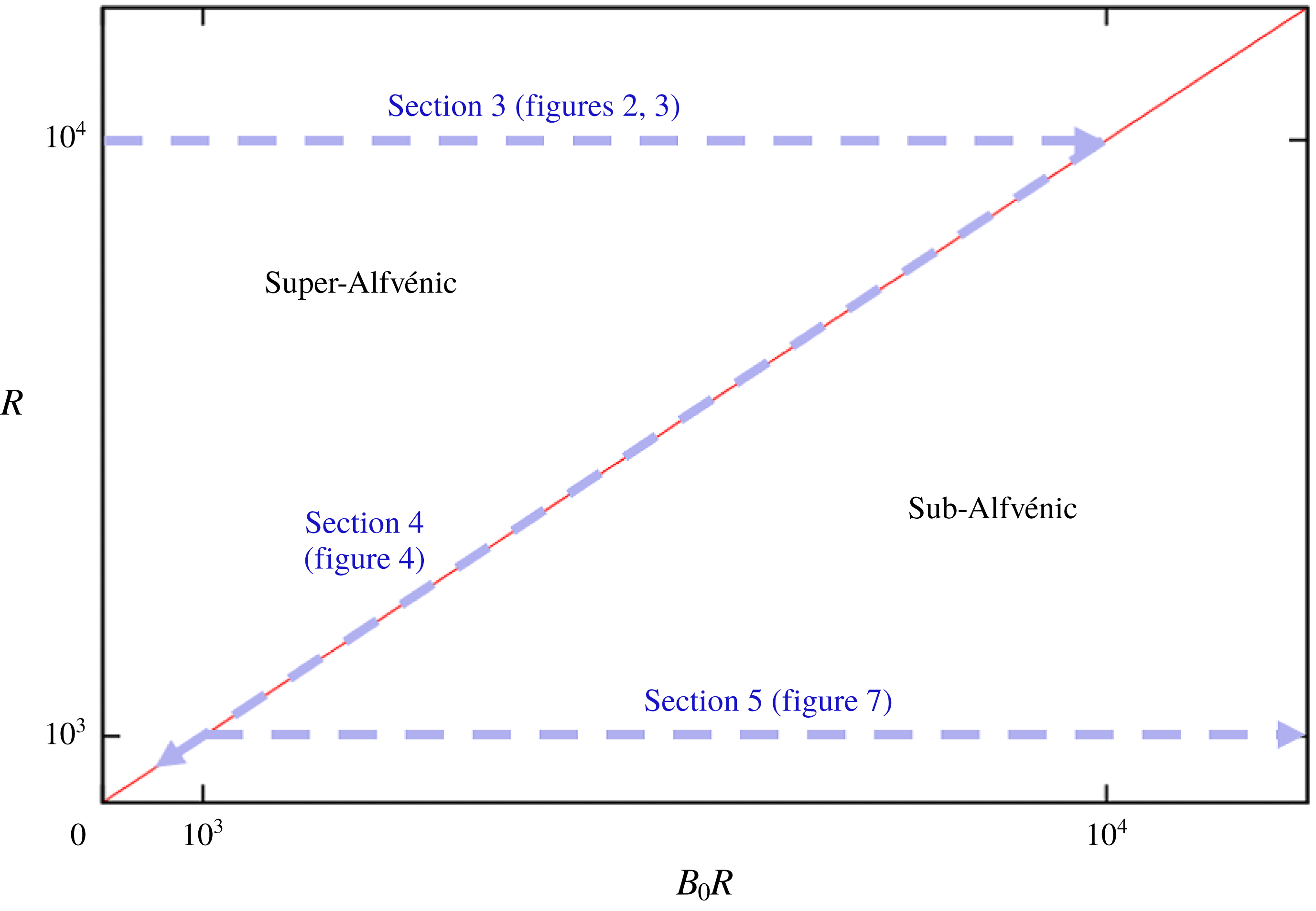
The parameter range explored in this paper. The vertical axis is the Reynolds number
 $R$
, which measures the strength of the base shear relative to the viscous effect. The horizontal axis is
 $B_{0}R$
, i.e. the same quantity but for the base magnetic field. The red diagonal line is the Chandrasekhar state
 $B_{0}=1$
. The region above this line is called the super-Alfvénic regime (
 $B_{0}<1$
), while below this line we have the sub-Alfvénic regime (
 $B_{0}>1$
).

After formulating the problem in the next section, we begin our numerical and theoretical analyses in §§ 3–5. The parameter range studied in those sections is summarised in figure 1. The first half of § 3 briefly reviews the numerical result of Deguchi (Reference Deguchi2019b
) where the nonlinear solutions are found for the super-Alfvénic regime using perfectly insulating walls. In the same section, we repeat the same computation but with perfectly conducting walls. In the latter case, the solution branch can be continued slightly beyond the Chandrasekhar limit. Section 4 analyses the Chandrasekhar flow in detail, using the energy equations. In § 5 we study the sub-Alfvénic solutions using small
 $P_{m}$
to show that the solution branch exists for very large
 $B_{0}$
. Finally, § 6 discusses some conclusions.
2 Formulation of the problem
Consider the non-dimensional viscous–resistive MHD equations
 $$\begin{eqnarray}\displaystyle & \displaystyle (\unicode[STIX]{x2202}_{t}+\boldsymbol{V}\boldsymbol{\cdot }\unicode[STIX]{x1D735})\boldsymbol{V}-(\boldsymbol{B}\boldsymbol{\cdot }\unicode[STIX]{x1D735})\boldsymbol{B}=-\unicode[STIX]{x1D735}Q+R^{-1}\unicode[STIX]{x1D6FB}^{2}\boldsymbol{V}, & \displaystyle\end{eqnarray}$$
 $$\begin{eqnarray}\displaystyle & \displaystyle (\unicode[STIX]{x2202}_{t}+\boldsymbol{V}\boldsymbol{\cdot }\unicode[STIX]{x1D735})\boldsymbol{B}-(\boldsymbol{B}\boldsymbol{\cdot }\unicode[STIX]{x1D735})\boldsymbol{V}=R_{m}^{-1}\unicode[STIX]{x1D6FB}^{2}\boldsymbol{B}, & \displaystyle\end{eqnarray}$$
 $$\begin{eqnarray}\displaystyle & \displaystyle \unicode[STIX]{x1D735}\boldsymbol{\cdot }\boldsymbol{V}=0,\quad \unicode[STIX]{x1D735}\boldsymbol{\cdot }\boldsymbol{B}=0, & \displaystyle\end{eqnarray}$$
where
 $\unicode[STIX]{x1D735}=(\unicode[STIX]{x2202}_{x},\unicode[STIX]{x2202}_{y},\unicode[STIX]{x2202}_{z})$
,
 $\boldsymbol{V}$
is the velocity,
 $\boldsymbol{B}$
is the magnetic field and
 $Q$
is the sum of the pressure and the magnetic pressure. We choose the velocity and length scales from the typical scales of the base flow (1.1). For the magnetic field, the corresponding Alfvén velocity is normalised by the velocity scale. The Reynolds number
 $R$
is the inverse of the kinematic viscosity normalised by the velocity and length scales. The magnetic Reynolds number
 $R_{m}$
is equal to
 $RP_{m}$
, where the magnetic Prandtl number
 $P_{m}$
is the ratio of the kinematic and magnetic diffusivities.
The specific flow configuration we choose is the plane Couette flow driven by mutually moving walls placed at
 $y=\pm 1$
. The base flow solution is
 $\boldsymbol{V}_{b}=U_{b}(y)\boldsymbol{i}$
with
 $U_{b}(y)=y$
, where
 $\boldsymbol{i}$
is the unit vector pointing in the direction of the generated flow. We take this direction to be an
 $x$
coordinate. For the velocity perturbation
 $\boldsymbol{v}=\boldsymbol{V}-\boldsymbol{V}_{b}=[u,v,w]$
we apply the no-slip conditions
 $\boldsymbol{v}=\mathbf{0}$
on the walls. The boundary conditions for the magnetic perturbation
 $\boldsymbol{b}=\boldsymbol{B}-\boldsymbol{B}_{b}=[a,b,c]$
are more complicated as they are dependent on the conductivity of the walls (Roberts Reference Roberts1964). We consider two popularly used extreme cases investigated in magnetised Taylor–Couette flow studies (see Rüdiger et al.
Reference Rüdiger, Schultz, Stefani and Mond2015; Gellert et al.
Reference Gellert, Rüdiger, Schultz, Guseva and Hollerbach2016; Rüdiger et al.
Reference Rüdiger, Gellert, Hollerbach, Schultz and Stefani2018), namely the perfectly conducting conditions
 $$\begin{eqnarray}\displaystyle \boldsymbol{n}\boldsymbol{\cdot }\boldsymbol{b}=\boldsymbol{n}\times (\unicode[STIX]{x1D735}\times \boldsymbol{b})=0\quad \text{at the walls} & & \displaystyle\end{eqnarray}$$
and the perfectly insulating conditions
 $$\begin{eqnarray}\displaystyle \boldsymbol{b}=\unicode[STIX]{x1D735}\unicode[STIX]{x1D711}\quad \text{at the walls}. & & \displaystyle\end{eqnarray}$$
Here,
 $\boldsymbol{n}$
is the unit vector normal to the wall and
 $\unicode[STIX]{x1D711}$
is the outer magnetic potential, which satisfies
 $\unicode[STIX]{x1D6FB}^{2}\unicode[STIX]{x1D711}=0$
in the outer domain (
 $y>1$
and
 $y<-1$
).
The equations for the perturbations are (the pressure perturbation is denoted as
 $q$
)
 $$\begin{eqnarray}\displaystyle & \displaystyle (\unicode[STIX]{x2202}_{t}+U_{b}\unicode[STIX]{x2202}_{x}+\boldsymbol{v}\boldsymbol{\cdot }\unicode[STIX]{x1D735}-R^{-1}\unicode[STIX]{x1D6FB}^{2})\boldsymbol{v}-(B_{0}U_{b}\unicode[STIX]{x2202}_{x}+\boldsymbol{b}\boldsymbol{\cdot }\unicode[STIX]{x1D735})\boldsymbol{b}+U_{b}^{\prime }(v-B_{0}b)\boldsymbol{i}=-\unicode[STIX]{x1D735}q,\quad & \displaystyle\end{eqnarray}$$
 $$\begin{eqnarray}\displaystyle & \displaystyle (\unicode[STIX]{x2202}_{t}+U_{b}\unicode[STIX]{x2202}_{x}+\boldsymbol{v}\boldsymbol{\cdot }\unicode[STIX]{x1D735}-R_{m}^{-1}\unicode[STIX]{x1D6FB}^{2})\boldsymbol{b}-(B_{0}U_{b}\unicode[STIX]{x2202}_{x}+\boldsymbol{v}\boldsymbol{\cdot }\unicode[STIX]{x1D735})\boldsymbol{v}+U_{b}^{\prime }(B_{0}v-b)\boldsymbol{i}=0,\quad & \displaystyle\end{eqnarray}$$
 $$\begin{eqnarray}\displaystyle & \displaystyle \unicode[STIX]{x1D735}\boldsymbol{\cdot }\boldsymbol{v}=\unicode[STIX]{x1D735}\boldsymbol{\cdot }\boldsymbol{b}=0. & \displaystyle\end{eqnarray}$$
 $x$
and
 $z$
directions with respective wavenumbers
 $\unicode[STIX]{x1D6FC}$
and
 $\unicode[STIX]{x1D6FD}$
. Unless otherwise stated,
 $\unicode[STIX]{x1D6FC}=1$
and
 $\unicode[STIX]{x1D6FD}=2$
; the corresponding computational box is
 $[0,2\unicode[STIX]{x03C0}]\times [-1,1]\times [0,\unicode[STIX]{x03C0}]$
. The periodicity of the domain allows us to use the toroidal–poloidal potential decomposition for the divergence-free fields:
 $$\begin{eqnarray}\left[\begin{array}{@{}c@{}}u\\ v\\ w\end{array}\right]=\left[\begin{array}{@{}c@{}}\overline{\overline{u}}+\unicode[STIX]{x1D719}_{xy}+\unicode[STIX]{x1D713}_{z}\\ -\unicode[STIX]{x1D719}_{xx}-\unicode[STIX]{x1D719}_{zz}\\ \overline{\overline{w}}+\unicode[STIX]{x1D719}_{yz}-\unicode[STIX]{x1D713}_{x}\end{array}\right],\quad \left[\begin{array}{@{}c@{}}a\\ b\\ c\end{array}\right]=\left[\begin{array}{@{}c@{}}\overline{\overline{a}}+f_{xy}+g_{z}\\ -f_{xx}-f_{zz}\\ \overline{\overline{c}}+f_{yz}-g_{x}\end{array}\right].\end{eqnarray}$$
Here the double overline represents the average in
 $x$
and
 $z$
, and so the mean fields
 $\overline{\overline{u}},\overline{\overline{w}},\overline{\overline{a}},\overline{\overline{c}}$
are functions of
 $y$
only. The poloidal potentials
 $\unicode[STIX]{x1D719},f$
and the toroidal potentials
 $\unicode[STIX]{x1D713},g$
are expanded by Fourier series in the two periodic directions:
 $$\begin{eqnarray}\unicode[STIX]{x1D719}=\mathop{\sum }_{m,n}\widehat{\unicode[STIX]{x1D719}}_{m,n}(y)\text{e}^{\text{i}m\unicode[STIX]{x1D6FC}x+\text{i}n\unicode[STIX]{x1D6FD}z},\quad \unicode[STIX]{x1D713}=\mathop{\sum }_{m,n}\widehat{\unicode[STIX]{x1D713}}_{m,n}(y)\text{e}^{\text{i}m\unicode[STIX]{x1D6FC}x+\text{i}n\unicode[STIX]{x1D6FD}z},\end{eqnarray}$$
 $$\begin{eqnarray}f=\mathop{\sum }_{m,n}\widehat{f}_{m,n}(y)\text{e}^{\text{i}m\unicode[STIX]{x1D6FC}x+\text{i}n\unicode[STIX]{x1D6FD}z},\quad g=\mathop{\sum }_{m,n}\widehat{g}_{m,n}(y)\text{e}^{\text{i}m\unicode[STIX]{x1D6FC}x+\text{i}n\unicode[STIX]{x1D6FD}z}.\end{eqnarray}$$
For the
 $y$
direction we use the collocation method with the modified Chebyshev basis functions carefully chosen to satisfy the boundary conditions. The boundary conditions for the Fourier coefficients are
 $$\begin{eqnarray}\widehat{\unicode[STIX]{x1D719}}_{m,n}=\unicode[STIX]{x2202}_{y}\widehat{\unicode[STIX]{x1D719}}_{m,n}=\widehat{\unicode[STIX]{x1D713}}_{m,n}=\overline{\overline{u}}=\overline{\overline{w}}=0\quad \text{at }y=\pm 1\end{eqnarray}$$
for the hydrodynamic components. Hence the appropriate basis functions for
 $\widehat{\unicode[STIX]{x1D719}}_{m,n}$
and (
 $\widehat{\unicode[STIX]{x1D713}}_{m,n},\overline{\overline{u}},\overline{\overline{w}}$
) are
 $$\begin{eqnarray}\displaystyle {\mathcal{B}}_{l}^{(1)}=(1-y^{2})^{2}T_{l}\quad \text{and}\quad {\mathcal{B}}_{l}^{(2)}=(1-y^{2})T_{l}, & & \displaystyle\end{eqnarray}$$
respectively, where
 $T_{l}(y)$
is the
 $l$
th Chebyshev polynomials.
When perfectly insulating walls are used, Deguchi (Reference Deguchi2019b ) showed that
 $$\begin{eqnarray}\displaystyle \unicode[STIX]{x2202}_{y}\widehat{f}_{m,n}\pm \sqrt{L}\,\widehat{f}_{m,n}=\widehat{g}_{m,n}=\overline{\overline{a}}=\overline{\overline{c}}=0\quad \text{at }y=\pm 1, & & \displaystyle\end{eqnarray}$$
where
 $L=(m\unicode[STIX]{x1D6FC})^{2}+(n\unicode[STIX]{x1D6FD})^{2}$
must be satisfied. Thus we can employ
 ${\mathcal{B}}_{l}^{(2)}$
to expand (
 $\widehat{g}_{m,n},\overline{\overline{a}},\overline{\overline{c}}$
) whilst for
 $\widehat{f}_{m,n}$
the basis functions can be chosen as
 $$\begin{eqnarray}\displaystyle {\mathcal{B}}_{l,m,n}^{(3)}={\mathcal{B}}_{l}^{(2)}+\frac{1+(-1)^{l}}{\sqrt{L}}+\frac{1-(-1)^{l}}{\sqrt{L}+1}y & & \displaystyle\end{eqnarray}$$
so that
 $\unicode[STIX]{x2202}_{y}{\mathcal{B}}_{l,m,n}^{(3)}\pm \sqrt{L}{\mathcal{B}}_{l,m,n}^{(3)}=0$
is satisfied.
The appropriate boundary conditions for the perfectly conducting case are
 $$\begin{eqnarray}\displaystyle \widehat{f}_{m,n}=\unicode[STIX]{x2202}_{y}\widehat{g}_{m,n}=\unicode[STIX]{x2202}_{y}\overline{\overline{a}}=\unicode[STIX]{x2202}_{y}\overline{\overline{c}}=0\quad \text{at }y=\pm 1. & & \displaystyle\end{eqnarray}$$
(In order to ensure (2.2),
 $\unicode[STIX]{x2202}_{y}^{2}\widehat{f}_{m,n}=0$
must also be satisfied on the walls. However this condition is automatically satisfied from the
 $y$
component of the induction equations.) Thus the basis
 ${\mathcal{B}}_{l}^{(2)}$
can be used to expand
 $\widehat{f}_{m,n}$
. For (
 $\widehat{g}_{m,n},\overline{\overline{a}},\overline{\overline{c}}$
), we can for example use the basis functions
 $$\begin{eqnarray}\displaystyle {\mathcal{B}}_{l}^{(4)}={\mathcal{B}}_{l}^{(2)}+(1-(-1)^{l})y+(1+(-1)^{l})\frac{2y^{2}-1}{4}, & & \displaystyle\end{eqnarray}$$
satisfying
 $\unicode[STIX]{x2202}_{y}{\mathcal{B}}_{l}^{(4)}=0$
on the walls.
The discretisation yields algebraic equations that can be solved by the multidimensional Newton method. The methodology allows us to continue the solution branches in the parameter space, without regarding their stability. Deguchi (Reference Deguchi2019b
) studied MHD solutions for non-rotating shear flows at large
 $R$
, while the earlier works by Rincon et al. (Reference Rincon, Ogilvie and Proctor2007) and Riols et al. (Reference Riols, Rincon, Cossu, Lesur, Longaretti, Ogilvie and Herault2013) concerned a system rotation effect in addition to the shear. Vaz, Boshier & Mestel (Reference Vaz, Boshier and Mestel2018) also used a similar method to find a dynamo solution for more idealised infinite cylindrical flows. The dynamo solutions found in Deguchi (Reference Deguchi2019a
) and in this paper are more similar to the shear-driven dynamos studied in Cline, Brummell & Cattaneo (Reference Cline, Brummell and Cattaneo2003), Yousef et al. (Reference Yousef, Heinemann, Schekochihin, Kleeorin, Rogachevskii, Iskakov, Cowley and McWilliams2008), Tobias & Cattaneo (Reference Tobias and Cattaneo2013) and Teed & Proctor (Reference Teed and Proctor2017), although unlike those previous studies there is no external body forcing term introduced here.
The steady solution found in Deguchi (Reference Deguchi2019b ) has the symmetries
 $$\begin{eqnarray}\displaystyle [u,v,w,a,b,c](x,y,z) & = & \displaystyle [-u,-v,w,-a,-b,c](-x,-y,z+\unicode[STIX]{x03C0}/\unicode[STIX]{x1D6FD})\nonumber\\ \displaystyle & = & \displaystyle [u,v,-w,a,b,-c](x+\unicode[STIX]{x03C0}/\unicode[STIX]{x1D6FC},y,-z).\end{eqnarray}$$
Throughout the nonlinear computations, the number of unknowns is reduced using those symmetries. For more details of the code, see Deguchi (Reference Deguchi2019b
). Typically 120 Chebyshev polynomials are used in
 $y$
, while 4 and 30 Fourier modes are used for
 $x$
and
 $z$
, respectively. In order to resolve the upper-branch state shown in figure 4, the number of streamwise Fourier modes is increased to 24.
As with most of the previous plane Couette flow studies, we use the shear on the wall to measure the deviation of a nonlinear solution from the basic laminar solution:
 $$\begin{eqnarray}\displaystyle \unicode[STIX]{x1D6E5}\equiv u_{y}|_{y=1}-1. & & \displaystyle\end{eqnarray}$$
The laminar solution has
 $\unicode[STIX]{x1D6E5}=0$
, while nonlinear solutions must have
 $\unicode[STIX]{x1D6E5}>0$
. One can alternatively choose a suitably defined amplitude of the perturbation, but here we prefer to use the physically important and experimentally measurable quantity.
The code can also be used to analyse the linear stability of the base flow with a little modification. To the best of the author’s knowledge, there is no unstable mode found for either magnetic boundary condition.
3 Super-Alfvénic cases
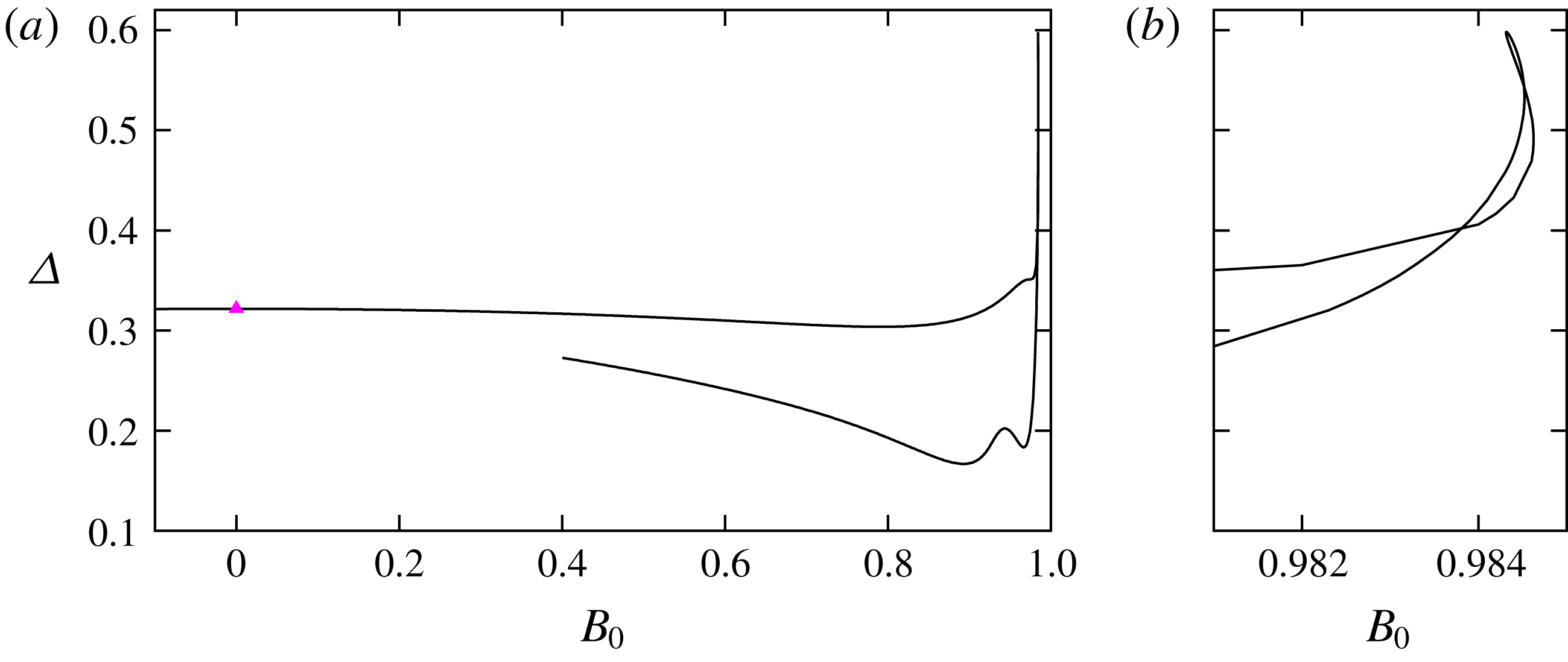
The bifurcation diagram of nonlinear steady solution in magnetised plane Couette flow with perfectly insulating walls. Here
 $(R,P_{m},\unicode[STIX]{x1D6FC},\unicode[STIX]{x1D6FD})=(10\,000,1,1,2)$
. This is the same result as Deguchi (Reference Deguchi2019b
, figure 7). The magenta triangle at
 $B_{0}=0$
is the NBC solution. The bifurcation diagram is symmetric with respect to
 $B_{0}=0$
. (b) is a close-up of (a) near the Chandrasekhar state
 $B_{0}=1$
.


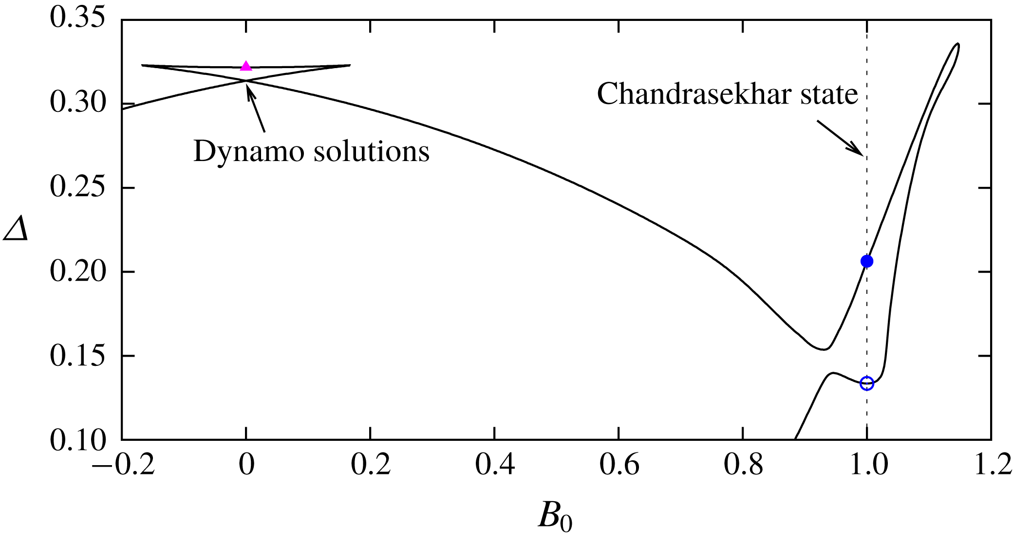
The bifurcation diagram for the Chandrasekhar state
 $B_{0}=1$
. Perfectly conducting walls are used. The solid curve is the sinuous mode, while the dashed curve is the mirror-symmetric mode.

In Deguchi (Reference Deguchi2019b
), various external magnetic fields were applied to plane Couette flow using perfectly insulating walls and
 $P_{m}=1$
; the flow (1.1) corresponds to the case where the spanwise uniform current is applied. The bifurcation diagram obtained in that paper is reproduced in figure 2. Here
 $\unicode[STIX]{x1D6E5}$
is the deviation of the drag on the wall from the laminar value, defined in (2.14). The start point of the computation is the NBC solution found for a purely hydrodynamic set-up by Nagata (Reference Nagata1990) and Clever & Busse (Reference Clever and Busse1992); the solution is shown by the magenta triangle at
 $B_{0}=0$
in the figure. The magnetised solution was referred to as the sinuous mode in Deguchi (Reference Deguchi2019b
), because it has symmetries (2.13) that generate three-dimensional sinusoidal fluid motion and magnetic field. The solution branch can be continued by the Newton method until we encounter the sharp turning point at
 $B_{0}=0.9846$
, which is very close to the Chandrasekhar limit
 $B_{0}=1$
. The branch then returns to the unmagnetised limit
 $B_{0}=0$
to produce a dynamo, but the branch is truncated in the figure for the sake of clarity (the major aim of the computation in Deguchi (Reference Deguchi2019b
) was to produce a dynamo solution at
 $B_{0}=0$
).
The main interest here is the singular behaviour of the solution branch around
 $B_{0}=1$
, which acts as a barrier in the continuation. That barrier also exists for other choices of
 $R$
and wavenumbers, and apparently the solution cannot be continued for the sub-Alfvénic regime. This phenomenon reminds us of the statement of the Chandrasekhar theorem; however, conditions (i) and (iii) mentioned in § 1 are not satisfied. This raises the question of whether we could extend the theory to show the non-existence of nonlinear solutions. In view of the MRI study by Rüdiger et al. (Reference Rüdiger, Schultz, Stefani and Mond2015), the choice
 $P_{m}=1$
would be crucial in finding the extension.
In Chandrasekhar’s theorem the condition (iii) can be replaced by the perfectly conducting conditions. Thus the effect of the conductivity of the walls on the nonlinear solutions is worth checking. Figure 3 is the same continuation result as figure 2 but with perfectly conducting walls. As seen in the figure, the behaviour of the branch is more complicated than for the insulating case. First, with increasing
 $B_{0}$
from the NBC state, the solution branch soon experiences the turning point at
 $B_{0}=0.17$
, and then returns to the unmagnetised limit. The new solution at
 $B_{0}=0$
maintains a magnetic field so it is a dynamo solution. There should be another dynamo solution with opposite polarity there, because of the symmetry of the MHD equations. However, the symmetry becomes imperfect for non-zero
 $B_{0}$
, and hence the behaviour of the other solution branch for
 $B_{0}>0$
is different from that of the previous branch. We can continue the new branch further up to
 $B_{0}=1.15$
beyond the Chandrasekhar limit. This is a rather unexpected result, because from Chandrasekhar’s theorem, one may think that the perfectly conducting case is more stable than the perfectly insulating case. In fact, Rüdiger et al. (Reference Rüdiger, Schultz, Stefani and Mond2015) found instability for the perfectly insulating case, while the flow seems to be stable when perfectly conducting walls are used.
Also, the large-Reynolds-number asymptotic theory by Deguchi (Reference Deguchi2019a
) suggests that the condition (ii) may not be satisfied as well. The assumption (ii) is only valid for large Reynolds numbers, but the largeness of
 $R$
does not mean diffusivity is negligible in the asymptotic limit. Deguchi (Reference Deguchi2019b
) confirmed that the Reynolds number of 10 000 used in the figure is sufficiently large so as to be able to employ the asymptotic result by Deguchi (Reference Deguchi2019a
), called the vortex–Alfvén wave interaction theory. The theory uses the mean-fluctuation decomposition; hereafter the
 $x$
-averaged part is called the roll-streak part (or the vortex part), and the fluctuation part is called the wave part. As was also shown in the hydrodynamic study by Hall & Sherwin (Reference Hall and Sherwin2010) for both components the diffusivity is not negligible. The roll-streak equations are fully diffusive, because the main convection mechanism in those equations is from the sweeping by the roll flow (i.e. the cross-streamwise components of the roll-streak part), which is much weaker than the base flow. For the wave part the ideal approximation can be used almost everywhere. However, the diffusivity is the leading-order effect within a thin layer around the singular point of the ideal problem. The mechanism by which the singular behaviour of the flow is reconciled within a thin diffusion layer surrounding the singular point is well known in the plasma physics community; see Sakurai, Goossens & Hollweg (Reference Sakurai, Goossens and Hollweg1991) and Goossens, Ruderman & Hollweg (Reference Goossens, Ruderman and Hollweg1995) for examples.
In the next section, we develop a theory to explain the numerical result obtained in this section. Analysis of the energy budget helps us to see the effect of the boundary terms and the diffusion terms. We shall see that the key to resolving the above rather paradoxical result is that the energy input from the perfectly conducting boundary term vanishes only when the ideal approximation is used. Thus when diffusive effects are present, both conducting and insulating walls may cause instability. We will then use the vortex–Alfvén wave interaction theory to see a special structure appear in the perfectly insulating boundary terms when the roll-streak–wave decomposition is applied. This special structure leads us to show the non-existence of non-trivial asymptotic solutions when
 $P_{m}=1$
.
4 The Chandrasekhar limit
4.1 The energy budget in the full MHD equations
Let us set
 $B_{0}=1$
in (2.1) (the result is also valid for
 $B_{0}=-1$
by the symmetry of the MHD equations). Using the Elsässer variables
 $\boldsymbol{\unicode[STIX]{x1D702}}_{\pm }=\boldsymbol{v}\pm \boldsymbol{b}=[\unicode[STIX]{x1D709}_{\pm },\boldsymbol{\unicode[STIX]{x1D702}}_{\pm },\unicode[STIX]{x1D701}_{\pm }]$
, equations (2.1) can be transformed into
 $$\begin{eqnarray}\displaystyle & \displaystyle (\unicode[STIX]{x2202}_{t}+2U_{b}\unicode[STIX]{x2202}_{x}+\boldsymbol{\unicode[STIX]{x1D702}}_{+}\boldsymbol{\cdot }\unicode[STIX]{x1D735}-R^{-1}\unicode[STIX]{x1D6FB}^{2})\boldsymbol{\unicode[STIX]{x1D702}}_{-}=-\unicode[STIX]{x1D735}q+R^{-1}(1-P_{m}^{-1})\unicode[STIX]{x1D6FB}^{2}\boldsymbol{b}, & \displaystyle\end{eqnarray}$$
 $$\begin{eqnarray}\displaystyle & \displaystyle (\unicode[STIX]{x2202}_{t}+\boldsymbol{\unicode[STIX]{x1D702}}_{-}\boldsymbol{\cdot }\unicode[STIX]{x1D735}-R^{-1}\unicode[STIX]{x1D6FB}^{2})\boldsymbol{\unicode[STIX]{x1D702}}_{+}+2U_{b}^{\prime }\boldsymbol{\unicode[STIX]{x1D702}}_{-}\boldsymbol{i}=-\unicode[STIX]{x1D735}q-R^{-1}(1-P_{m}^{-1})\unicode[STIX]{x1D6FB}^{2}\boldsymbol{b}. & \displaystyle\end{eqnarray}$$
 $$\begin{eqnarray}\displaystyle E_{\pm }=\frac{\langle |\boldsymbol{\unicode[STIX]{x1D702}}_{\pm }|^{2}\rangle }{2}, & & \displaystyle\end{eqnarray}$$
where the angle brackets denote the spatial average over the computational domain
 $[0,2\unicode[STIX]{x03C0}/\unicode[STIX]{x1D6FC}]\times [-1,1]\times [0,2\unicode[STIX]{x03C0}/\unicode[STIX]{x1D6FD}]$
. Averaging
 $\boldsymbol{\unicode[STIX]{x1D702}}_{-}\boldsymbol{\cdot }(4.1a)$
and
 $\boldsymbol{\unicode[STIX]{x1D702}}_{+}\boldsymbol{\cdot }(4.1b)$
, we can derive two energy budget equations
 $$\begin{eqnarray}\displaystyle & \displaystyle \frac{\text{d}E_{-}}{\text{d}t}=-R^{-1}D_{-}-\unicode[STIX]{x1D6E4}+R^{-1}(\unicode[STIX]{x1D6EC}-\unicode[STIX]{x1D706})+R^{-1}(1-P_{m}^{-1})\langle \boldsymbol{\unicode[STIX]{x1D702}}_{-}\boldsymbol{\cdot }\unicode[STIX]{x1D6FB}^{2}\boldsymbol{b}\rangle , & \displaystyle\end{eqnarray}$$
 $$\begin{eqnarray}\displaystyle & \displaystyle \frac{\text{d}E_{+}}{\text{d}t}=2I-R^{-1}D_{+}+\unicode[STIX]{x1D6E4}+R^{-1}(\unicode[STIX]{x1D6EC}+\unicode[STIX]{x1D706})-R^{-1}(1-P_{m}^{-1})\langle \boldsymbol{\unicode[STIX]{x1D702}}_{+}\boldsymbol{\cdot }\unicode[STIX]{x1D6FB}^{2}\boldsymbol{b}\rangle . & \displaystyle\end{eqnarray}$$
 $$\begin{eqnarray}D_{\pm }=\langle |\unicode[STIX]{x1D735}\boldsymbol{\unicode[STIX]{x1D702}}_{\pm }|^{2}\rangle \quad \text{and}\quad I=-\langle U_{b}^{\prime }\boldsymbol{\unicode[STIX]{x1D702}}_{-}\unicode[STIX]{x1D709}_{+}\rangle\end{eqnarray}$$
are the diffusion term and the energy input term due to the base flow, respectively.
The boundary terms
 $$\begin{eqnarray}\unicode[STIX]{x1D6E4}=\frac{1}{2}\left[\overline{\overline{b\left(\frac{|\boldsymbol{b}|^{2}}{2}-q\right)}}\right]_{-1}^{1},\quad \unicode[STIX]{x1D6EC}=\frac{1}{2}\left[\overline{\overline{(aa_{y}+bb_{y}+cc_{y})}}\right]_{-1}^{1},\end{eqnarray}$$
 $$\begin{eqnarray}\unicode[STIX]{x1D706}={\textstyle \frac{1}{2}}[\overline{\overline{(au_{y}-cw_{y})}}]_{-1}^{1}\end{eqnarray}$$
may also act as an energy input mechanism (recall that the double overline is the
 $x$
–
 $z$
average). Those terms can be simplified by using the magnetic boundary conditions, as summarised in table 1. The assumption (iii) mentioned in § 1 essentially requires that all the boundary terms are negligibly small; this case may occur when the coherent structure is localised at the mid-channel (as seen in Deguchi (Reference Deguchi2015)), or the problem is considered in an unbounded domain. For the perfectly insulating case (2.3), all the boundary terms are non-zero. At perfectly conducting walls,
 $a_{y},c_{y}$
and
 $b$
must vanish from (2.2), and hence
 $\unicode[STIX]{x1D6E4}$
and
 $\unicode[STIX]{x1D6EC}$
must be zero, while
 $\unicode[STIX]{x1D706}$
may not be zero.

Under Chandrasekhar’s assumptions (i)–(iii), all the terms on the right-hand side of (4.3) can be dropped except for the energy input term
 $2I$
from the base flow. In the linear framework, a time derivative can be replaced by the exponential growth rate of the flow amplitude. From the first equation (4.3a
), clearly the velocity and magnetic field eigenfunctions must be identical to have a non-zero growth rate. However, from the second equation (4.3b
), this class of eigenfunctions must also have a zero growth rate, because
 $I\equiv 0$
. Therefore the Chandrasekhar theorem follows. Note that the only boundary term that survives in the diffusionless approximation is
 $\unicode[STIX]{x1D6E4}$
; therefore, as widely accepted, the theorem is valid for perfectly conducting conditions (see table 1).
We further remark here that for unidirectional flows the theorem can be used whatever the magnetic boundary conditions. From the linearised ideal induction equations, we can deduce that
 $(U_{b}-s)b=U_{b}v$
must hold, where
 $s$
is the complex phase speed of the wave. Therefore, except for the unlikely situation that the wave is neutral and its travelling speed coincides with the speed of the base flow on one of the walls,
 $b$
must vanish on the walls (and hence
 $\unicode[STIX]{x1D6E4}=0$
) as long as the impermeability conditions are satisfied there.
The mechanism of the linear instability seen in Rüdiger et al. (Reference Rüdiger, Schultz, Stefani and Mond2015) can be explained using (4.3). When
 $P_{m}=1$
, the stability result is consistent with the Chandrasekhar theorem, and hence the stability property can be explained by the ideal mechanism. However, the existence of the instability for
 $P_{m}\neq 1$
suggests that the terms multiplied by
 $(1-P_{m}^{-1})$
in (4.3) have some destabilisation effects. Those terms indeed play a role when a singularity occurs in the ideal problem, even when the instability is predominantly driven by some ideal mechanism almost everywhere (e.g. Bogdanova-Ryzhova & Ryzhov Reference Bogdanova-Ryzhova and Ryzhov1994; Sakurai et al.
Reference Sakurai, Goossens and Hollweg1991). The absorption of the wave at the singularity occurs in a small scale, and hence the derivative of the flow appearing in the corresponding terms in (4.3) may not be small.
Now we turn our attention to the nonlinear regime. The stability of the Chandrasekhar state can actually be shown even when nonlinearity and diffusivity are present in the flow. More precisely, the assumptions (i) and (ii) are not necessary to prove the stability, as long as
 $P_{m}=B_{0}=1$
and the assumption (iii) is satisfied. The proof of this new result follows from (4.3a
) and the total energy equation, which can be obtained for example by adding (4.3a
) and (4.3b
):
 $$\begin{eqnarray}\displaystyle \frac{\text{d}E}{\text{d}t}=I-R^{-1}D, & & \displaystyle\end{eqnarray}$$
where
 $E=(\langle |\boldsymbol{v}|^{2}+|\boldsymbol{b}|^{2}\rangle /2)+{\mathcal{E}}\geqslant 0$
and
 $D=\langle |\unicode[STIX]{x1D735}\boldsymbol{v}|^{2}+|\unicode[STIX]{x1D735}\boldsymbol{b}|^{2}\rangle +{\mathcal{D}}\geqslant 0$
. The functions
 ${\mathcal{E}}$
and
 ${\mathcal{D}}$
are defined in appendix A; they have come from the boundary term
 $\unicode[STIX]{x1D6EC}$
, and
 $D=E=0$
occurs only for the trivial solution. The other boundary terms
 $\unicode[STIX]{x1D6E4}$
and
 $\unicode[STIX]{x1D706}$
are cancelled out. When (iii) is satisfied, there is no energy input term in (4.3a
) and thus
 $E_{-}$
must decay monotonically; thus the equipartitioned state
 $\boldsymbol{v}=\boldsymbol{b}$
is realised ultimately. Approaching the equipartition state the shear energy input term behaves like
 $I\rightarrow 0$
. If
 $I=0$
, from (4.6) we can show that
 $E$
is a Lyapunov function of the base state in the entire phase space.
The extended version of the Chandrasekhar theorem above implies that if a non-trivial nonlinear state exists in the Chandrasekhar state, the magnetic perturbation generated by it should strongly interact with the walls. Unlike the original Chandrasekhar theorem, the extended result is not valid when (iii) is replaced by perfectly conducting conditions, because of the non-vanishing viscous boundary terms
 $\unicode[STIX]{x1D706}$
and
 $\unicode[STIX]{x1D6EC}$
. Also, for the perfectly insulating problem, the boundary terms hinder further theoretical progresses.
The next step we can take towards a theoretical understanding of the numerical result in § 3 is to apply some rational reduction to the governing equations. In § 4.3, we use the vortex–Alfvén wave interaction theory derived at the large-Reynolds-number limit for this purpose. Before the asymptotic analysis, in the next section, we give a detailed look at the nonlinear solutions found in the Chandrasekhar state using the perfectly conducting conditions. The examination of the flow structure computed at moderately large Reynolds number may also help the reader’s understanding of the asymptotic theory.
4.2 Nonlinear states at
 $P_{m}=B_{0}=1$
for the perfectly conducting conditions

For the perfectly conducting case, non-trivial solutions can be found even when
 $P_{m}=B_{0}=1$
as seen in § 3. Therefore, the best we can do in (4.6) for this case is to find the critical energy Reynolds number
 $R_{E}$
below which the laminar flow is globally stable. To compute
 $R_{E}$
, first the maximum of
 $I/D$
over all
 $\boldsymbol{b}$
and divergence-free
 $\boldsymbol{v}$
must be computed. The maximum
 $M$
can be found by solving the Euler–Lagrange equations
 $$\begin{eqnarray}U_{b}^{\prime }(v-b)=-q_{x}+2M\unicode[STIX]{x0394}u,\quad U_{b}^{\prime }(u+a)=-q_{y}+2M\unicode[STIX]{x0394}v,\quad 0=-q_{z}+2M\unicode[STIX]{x0394}w,\end{eqnarray}$$
 $$\begin{eqnarray}u_{x}+v_{y}+w_{z}=0,\quad U_{b}^{\prime }(v-b)=2M\unicode[STIX]{x0394}a,\quad U_{b}^{\prime }(u+a)=2M\unicode[STIX]{x0394}b,\end{eqnarray}$$
where
 $u=v=w=b=a_{y}=0$
at
 $y=\pm 1$
. The optimum perturbation found at
 $(\unicode[STIX]{x1D6FC},\unicode[STIX]{x1D6FD})=(1.79,0)$
gives the energy Reynolds number
 $R_{E}=M^{-1}=72.58$
. The value found is remarkably higher than that for purely hydrodynamic plane Couette flow (
 $(R_{E},\unicode[STIX]{x1D6FC},\unicode[STIX]{x1D6FD})=(20.66,0,1.56)$
; see Joseph (Reference Joseph1966)), implying that the magnetic field causes a stabilisation effect to the flow.
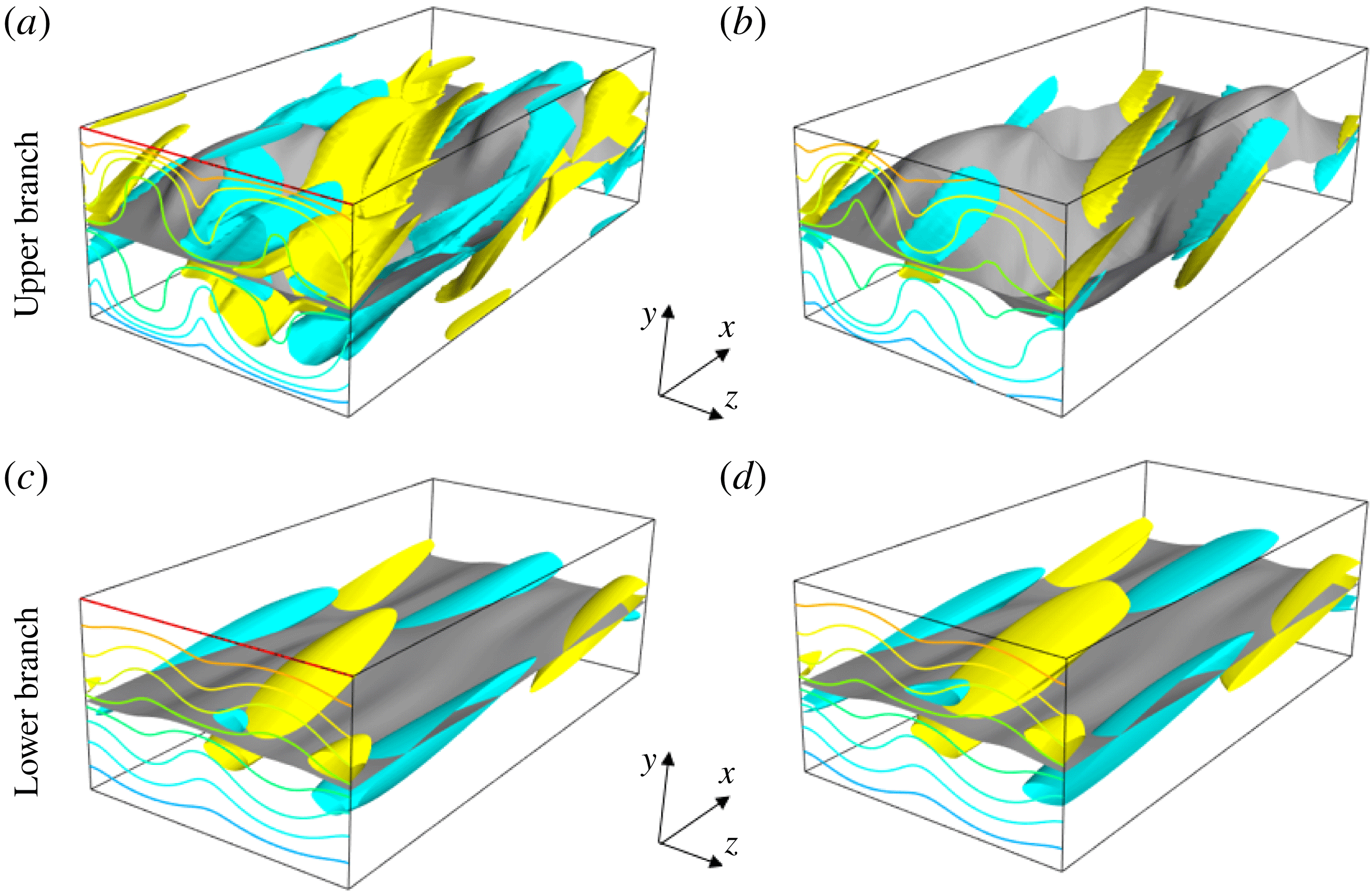
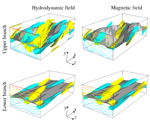
The flow visualisation of the mirror-symmetric nonlinear solutions seen in figure 4. The Chandrasekhar state at
 $R=1000$
. The (a,c) left- and (b,d) right-hand panels show the hydrodynamic and magnetic fields, respectively. Yellow and blue represent isosurface of 50 % streamwise vorticity (current) which are dominated by the wave component excited by the resonance occurring at the middle of the channel. The grey surface is the zero of the streamwise velocity (magnetic field). The contour of the hydrodynamic (magnetic) streak is also shown at the front of the computational box (
 $[0,2\unicode[STIX]{x03C0}]\times [-1,1]\times [0,\unicode[STIX]{x03C0}]$
).

All non-trivial equilibrium solutions should exist for
 $R>R_{E}$
. This can be checked by varying
 $R$
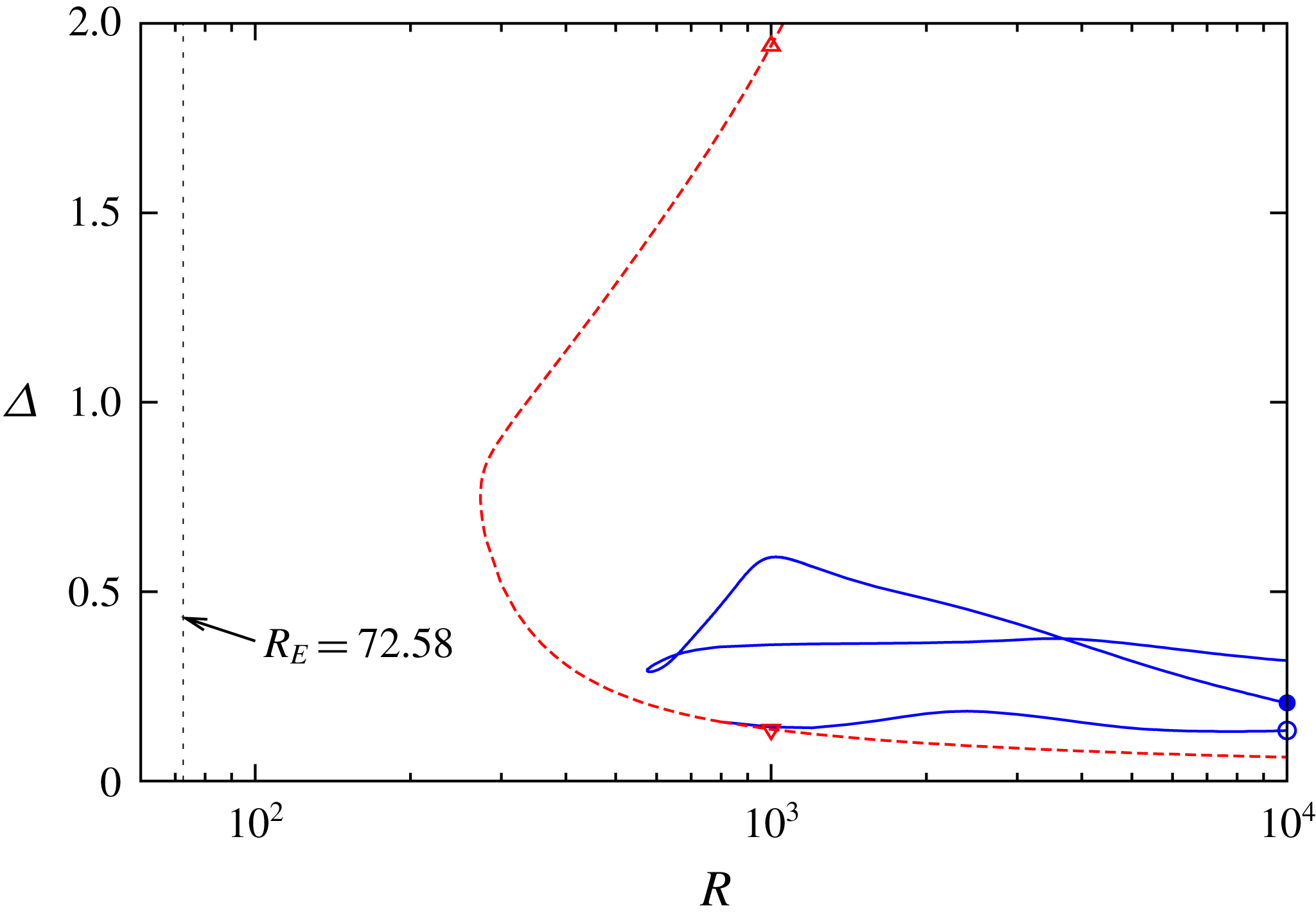
from the solutions obtained in figure 3. In figure 4 the bifurcation diagram for
 $B_{0}=P_{m}=1$
is shown. The two points marked by the open and filled circles are those seen in figure 3. From the upper point, we can trace the branch towards the saddle-node point at
 $R=575$
, but the turned branch does not return to the lower point. The branch continued from the lower point revealed that it is originated from the bifurcation point
 $R=802$
, at which the solid curve connects to the dashed curve. The solution on the dashed curve has the mirror symmetry
 $$\begin{eqnarray}\displaystyle ~[u,v,w,a,b,c](x,y,z)=[u,v,-w,a,b,-c](x,y,-z+\unicode[STIX]{x03C0}/\unicode[STIX]{x1D6FD}) & & \displaystyle\end{eqnarray}$$
in addition to (2.13) (the hydrodynamic part of the symmetry is the same as EQ7/EQ8 in Gibson, Halcrow & Cvitanovic (Reference Gibson, Halcrow and Cvitanovic2009) and Itano & Generalis (Reference Itano and Generalis2009)). In figure 4, blue solid curves are used for the sinuous mode that has the symmetry (2.13) but does not satisfy (4.8). This mirror-symmetric mode has a saddle-node point sitting at a lower Reynolds number (
 ${\approx}273$
) than that of the sinuous mode. Nevertheless, this value is much higher than that for the purely hydrodynamic plane Couette flow,
 $R\approx 162$
(see Deguchi Reference Deguchi2019a
).
Deguchi (Reference Deguchi2019b ) found that there are two typical types of asymptotic behaviours of the solutions at large Reynolds numbers. The upper and lower branches of the mirror-symmetric solution seen in figure 4 best illustrate the difference of those two.
For the lower branch, the shear
 $\unicode[STIX]{x1D6E5}$
seems to converge towards some constant with increasing
 $R$
. This is because the flow asymptotes to the vortex–Alfvén wave interaction type of state studied in Deguchi (Reference Deguchi2019a
,Reference Deguchi
b
); the sinuous mode solutions we have seen in figures 2 and 3 are also of this type. The lower panels of figure 5 display the structure of the lower-branch solution at
 $R=1000$
. The mechanism sustaining the solution can be explained by the asymptotic theory as follows. First we note in the figure that the grey surfaces showing the isosurface of the zero streamwise velocity field are almost flat (recall that the streamwise direction is
 $x$
). In fact, the velocity and magnetic fields are dominated by the
 $x$
average of the streamwise component, called the streak. The origin of the less dominant three-dimensional structure can be explained by the ideal linear neutral stability of that streak; therefore, only one streamwise Fourier mode is necessary to describe the leading-order structures. The structure of the lower-branch states is similar to the so-called alpha–omega dynamo, where the strong shear generates fields in the
 $x$
direction from transverse fields; meanwhile waves on the flow can give an alpha effect so that diffusion can sustain the transverse fields. The idea of using mean-fluctuation decomposition can be seen in various mean-field dynamo theories (Braginsky Reference Braginsky1964; Moffatt Reference Moffatt1978; Krause & Rädler Reference Krause and Rädler1980).
However, the vortex–Alfvén wave interaction theory is more than the mean-field theory, because the closure problem inevitably associated with the decomposition is rationally resolved by only assuming the largeness of the Reynolds number. The key to the resolution was the use of the matched asymptotic expansions. The stability problem possesses a singularity at the resonant position, where the velocity relative to the phase speed of the wave coincides with the Alfvén velocity. For the mirror-symmetric mode, by symmetry, the resonant position is simply
 $y=0$
, where the grey surface sits. The absorption of the Alfvén wave there creates the strong streamwise vortex and current shown by the blue and yellow surfaces. The vorticity/current is trapped within a thin diffusive layer, whose thickness gets thinner with increasing
 $R$
. The strong fluctuation emerging within the diffusive layer causes a nonlinear feedback effect to the
 $x$
-averaged field through the Reynolds stress. Thus the wave causes a strongly nonlinear feedback effect to the mean field, despite its rather simple structure in the streamwise direction. The entire mechanism outlined here is very similar to the purely hydrodynamic counterpart studied in Hall & Sherwin (Reference Hall and Sherwin2010), which can be found on the edge of laminar and turbulent attractors, as shown by Wang et al. (Reference Wang, Gibson and Waleffe2007).
For the upper branch, by contrast, the value of
 $\unicode[STIX]{x1D6E5}$
increases indefinitely for large
 $R$
(see figure 4). This asymptotic behaviour of
 $\unicode[STIX]{x1D6E5}$
is typical in turbulence simulations, due to the presence of a near-wall boundary-layer structure in the flow. In the upper panels of figure 5, where the upper-branch solution at
 $R=1000$
is visualised, the presence of the near-wall boundary layer structure can indeed be seen in the contour of the streamwise field shown at the front of the computational box. The streamwise velocity and magnetic fields are no longer dominated by the
 $x$
average, as can be seen in the strongly modulated wavy grey surfaces. The streamwise vorticity and current fields have very complicated structures spread out in the entire channel. The existence of a formal asymptotic theory for that complicated flow remains an open question.
4.3 Non-existence of the vortex–Alfvén wave interaction type of nonlinear states for perfectly insulating conditions
The large-Reynolds-number limit corresponds to the singular perturbation problem, and thus the limit of the diffusive problem may not coincide with the ideal results. Deguchi (Reference Deguchi2019a
) derived a set of reduced nonlinear equations by taking the large-Reynolds-number limit of the viscous–resistive MHD equations. We shall shortly see that the diffusivity is in fact not negligible in the limiting reduced leading-order problem. The aim of this section is to show that there is no nontrivial solution in the reduced problem when
 $B_{0}=P_{m}=1$
and the perfectly insulating conditions are used. That theoretical result may explain the numerical result obtained in figure 2.
The vortex–Alfvén wave interaction theory derived in Deguchi (Reference Deguchi2019a
) is valid for travelling-wave solutions propagating in
 $x$
with speed
 $s$
. The leading-order flow has the form
 $$\begin{eqnarray}\displaystyle & \displaystyle \boldsymbol{V}=U_{b}\boldsymbol{i}+[\overline{u}(y,z),R^{-1}\overline{v}(y,z),R^{-1}\overline{w}(y,z)]^{T}+\unicode[STIX]{x1D716}R^{-1}\{\widetilde{\boldsymbol{v}}(y,z)\text{e}^{\text{i}\unicode[STIX]{x1D6FC}(x-st)}+\text{c.c.}\}, & \displaystyle\end{eqnarray}$$
 $$\begin{eqnarray}\displaystyle & \displaystyle \boldsymbol{B}=U_{b}\boldsymbol{i}+[\overline{a}(y,z),R^{-1}\overline{b}(y,z),R^{-1}\overline{c}(y,z)]^{T}+\unicode[STIX]{x1D716}R^{-1}\{\widetilde{\boldsymbol{b}}(y,z)\text{e}^{\text{i}\unicode[STIX]{x1D6FC}(x-st)}+\text{c.c.}\}, & \displaystyle\end{eqnarray}$$
 $$\begin{eqnarray}\displaystyle & \displaystyle Q=R^{-2}\overline{q}(y,z)+\unicode[STIX]{x1D716}R^{-1}\{\widetilde{q}(y,z)\text{e}^{\text{i}\unicode[STIX]{x1D6FC}(x-st)}+\text{c.c.}\}. & \displaystyle\end{eqnarray}$$
 $x$
-averaged components called the ‘vortex’, or ‘roll-streak’, part; the streamwise and cross-streamwise components are referred to as the streak and roll, respectively. The ‘wave’ part is the component fluctuating in
 $x$
; the amplitude
 $\unicode[STIX]{x1D716}$
is to be specified later. Only one Fourier mode is needed in this component because it is determined by a linear stability of the streak field.
Substituting (4.9) into (2.1), and then applying the large-Reynolds-number asymptotic reduction, Deguchi (Reference Deguchi2019a
) found a closure for the leading-order solution. If
 $B_{0}$
and
 $P_{m}$
are both unity, the
 $x$
-average parts of the leading-order equations are
 $$\begin{eqnarray}\displaystyle & & \displaystyle [(\overline{v}\unicode[STIX]{x2202}_{y}+\overline{w}\unicode[STIX]{x2202}_{z})-\unicode[STIX]{x1D6FB}^{2}]\left[\begin{array}{@{}c@{}}\overline{u}\\ \overline{v}\\ \overline{w}\end{array}\right]-[\overline{b}\unicode[STIX]{x2202}_{y}+\overline{c}\unicode[STIX]{x2202}_{z}]\left[\begin{array}{@{}c@{}}\overline{a}\\ \overline{b}\\ \overline{c}\end{array}\right]+\left[\begin{array}{@{}c@{}}0\\ \overline{q}_{y}\\ \overline{q}_{z}\end{array}\right]\nonumber\\ \displaystyle & & \displaystyle \qquad =\left[\begin{array}{@{}c@{}}U_{b}^{\prime }(\overline{b}-\overline{v})\\ 0\\ 0\end{array}\right]-\frac{\unicode[STIX]{x1D716}^{2}}{\unicode[STIX]{x1D6FC}^{2}}\left[\begin{array}{@{}c@{}}0\\ \{(|\widetilde{v}|^{2}-|\widetilde{b}|^{2})_{y}+(\widetilde{v}\widetilde{w}-\widetilde{b}\widetilde{c})_{z}\}+\text{c.c.}\\ \{(|\widetilde{w}|^{2}-|\widetilde{c}|^{2})_{z}+(\widetilde{v}\widetilde{w}-\widetilde{b}\widetilde{c})_{y}\}+\text{c.c.}\end{array}\right],\end{eqnarray}$$
 $$\begin{eqnarray}[(\overline{v}\unicode[STIX]{x2202}_{y}+\overline{w}\unicode[STIX]{x2202}_{z})-\unicode[STIX]{x1D6FB}^{2}]\left[\begin{array}{@{}c@{}}\overline{a}\\ \overline{b}\\ \overline{c}\end{array}\right]-[\overline{b}\unicode[STIX]{x2202}_{y}+\overline{c}\unicode[STIX]{x2202}_{z}]\left[\begin{array}{@{}c@{}}\overline{u}\\ \overline{v}\\ \overline{w}\end{array}\right]=\left[\begin{array}{@{}c@{}}U_{b}^{\prime }(\overline{b}-\overline{v})\\ 0\\ 0\end{array}\right],\end{eqnarray}$$
 $$\begin{eqnarray}\overline{v}_{y}+\overline{w}_{z}=0,\quad \overline{b}_{y}+\overline{c}_{z}=0,\end{eqnarray}$$
whilst the fluctuation part becomes
 $$\begin{eqnarray}\left(\frac{\widetilde{q}_{y}}{(U-s)^{2}-A^{2}}\right)_{y}+\left(\frac{\widetilde{q}_{z}}{(U-s)^{2}-A^{2}}\right)_{z}-\unicode[STIX]{x1D6FC}^{2}\frac{\widetilde{q}}{(U-s)^{2}-A^{2}}=0.\end{eqnarray}$$
Equation (4.11) comes from the ideal linear stability problem of the hydrodynamic streak
 $U=U_{b}+\overline{u}$
, and the magnetic streak
 $A=U_{b}+\overline{a}$
. Having determined
 $\widetilde{q}$
, we can easily relate it to
 $\widetilde{\boldsymbol{v}}$
and
 $\widetilde{\boldsymbol{b}}$
. In particular,
 $$\begin{eqnarray}\widetilde{v}=-\frac{\widetilde{q}_{y}(U-s)}{i\unicode[STIX]{x1D6FC}((U-s)^{2}-A^{2})},\quad \widetilde{w}=-\frac{\widetilde{q}_{z}(U-s)}{i\unicode[STIX]{x1D6FC}((U-s)^{2}-A^{2})}\end{eqnarray}$$
and the ‘frozen’ condition
 $$\begin{eqnarray}\displaystyle (U-s)[\widetilde{b},\widetilde{c}]=A[\widetilde{v},\widetilde{w}] & & \displaystyle\end{eqnarray}$$
holds.
On a curve where either
 $\overline{u}-s=\overline{a}$
or
 $\overline{u}-s=-\overline{a}$
is satisfied,
 $(U-s)^{2}-A^{2}$
vanishes and hence equation (4.11) becomes singular. Around the critical curves at which the singularity occurs, we must retain the diffusive effects to regularise the flow. The thickness of the diffusion layer is
 $O(R^{-1/3})$
, which is well known in resonant absorption studies (Sakurai et al.
Reference Sakurai, Goossens and Hollweg1991; Goossens et al.
Reference Goossens, Ruderman and Hollweg1995). Two types of diffusion-layer structures were determined in Deguchi (Reference Deguchi2019a
) together with the appropriate wave amplitude
 $\unicode[STIX]{x1D716}$
. Type 1 occurs when the two diffusive layers are well separated; the amplitude in this case is
 $\unicode[STIX]{x1D716}=1$
. In type 2, the two diffusive layers merge so that the resonance there becomes stronger; as a consequence, a smaller size of the wave amplitude
 $\unicode[STIX]{x1D716}=R^{-1/6}$
must be used.
The sharp structure within the thin diffusive layer creates a jump in the derivative of the outer hydrodynamic roll components. The appropriate forms of the jump for types 1 and 2 were found in Deguchi (Reference Deguchi2019a ). Equations (4.10) and (4.11) form a closure valid at the large-Reynolds-number limit together with the jump condition.
Although the reduced equations may look complicated, the important point here is twofold; first, the wave fields
 $\widetilde{\boldsymbol{v}},\widetilde{\boldsymbol{b}}$
are generated by the ideal linear stability problem of the streak fields (4.11); second, there is no direct feedback from the wave to the streak as one can easily confirm in (4.10). Hence, the perturbation streak fields
 $\overline{u},\overline{a}$
are maintained indirectly through the roll fields driven by the wave field, which is induced by the instability of the streak. The three-point cyclic coupling between the wave, roll and streak fields is similar to that seen in the hydrodynamic theory (Hall & Smith Reference Hall and Smith1991; Wang et al.
Reference Wang, Gibson and Waleffe2007; Hall & Sherwin Reference Hall and Sherwin2010).
Now, let us show that there is no solution if the wall is perfectly insulating. The core of the theoretical result are the following cross-energy equations similar to (4.3) but for the perturbation Elsässer streak field
 $\overline{\unicode[STIX]{x1D709}}_{\pm }=\overline{u}\pm \overline{a}$
:
 $$\begin{eqnarray}\langle |\unicode[STIX]{x1D735}\overline{\unicode[STIX]{x1D709}}_{-}|^{2}\rangle =-\unicode[STIX]{x1D6FE}_{-},\quad \langle |\unicode[STIX]{x1D735}\overline{\unicode[STIX]{x1D709}}_{+}|^{2}\rangle =2{\mathcal{I}}-\unicode[STIX]{x1D6FE}_{+},\end{eqnarray}$$
where
 ${\mathcal{I}}=-\langle U_{b}^{\prime }\overline{v}\overline{\unicode[STIX]{x1D709}}_{+}\rangle$
and
 $$\begin{eqnarray}\unicode[STIX]{x1D6FE}_{\pm }=\frac{1}{2}\left[\overline{\overline{\overline{a}\overline{\unicode[STIX]{x1D709}}_{\pm }}}\right]_{-1}^{1}.\end{eqnarray}$$
Those equations can be derived by the
 $x$
components of (4.10). As remarked earlier, there is no energy input from the wave activity, because of the asymptotic reduction. Thus, the diffusion terms on the left-hand side of (4.14) are maintained by the roll energy input term
 ${\mathcal{I}}$
and the boundary terms
 $\unicode[STIX]{x1D6FE}_{\pm }$
.
For the insulating case, the magnetic streak
 $\overline{a}=\overline{\overline{a}}+\overline{g}_{z}$
must vanish on the walls, from (2.5) and (2.9). Thus there is no contribution from the the boundary terms
 $\unicode[STIX]{x1D6FE}_{\pm }$
. From the first equation in (4.14), we see that the streak components must satisfy the equipartition condition
 $\overline{u}=\overline{a}$
. We then recall that the wave component is generated through the ideal linear stability problem of the streak. Thus, we can show by the generalised version of Chandrasekhar’s theorem that there is no wave component generated from the equipartitioned streaks (see § 4.1). Without the wave, the roll component cannot be maintained, and thus
 ${\mathcal{I}}=0$
. Therefore, using (4.14) again, we arrive at the conclusion that the perturbation streaks
 $\overline{u}$
and
 $\overline{a}$
must be identically zero (more technical details of the discussion here can be found in appendix B).
The discussion above critically relies on the behaviour of the boundary terms in the streak energy equations (4.14). For perfectly conducting walls,
 $\overline{a}$
is non-vanishing on the walls, and hence the equipartitioned streaky fields are not realised, as indeed can be seen in figure 5. This may be the reason why we can compute nonlinear solutions even when
 $B_{0}=P_{m}=1$
.
We close this section by noting that the mechanism behind the equipartitioning of the streaky fields is somewhat similar to the Reynolds analogy seen in stratified shear flows (i.e. the mean temperature is approximately proportional to the mean streamwise velocity when the Prandtl number is close to unity). In fact, the analysis in § 3 is very similar to that in Deguchi (Reference Deguchi2017), where the vortex–wave interaction theory was applied for stratified plane Couette flow and it was found that the Reynolds analogy exactly holds. This result and the outcome in this section are good examples showing the usefulness of the asymptotic reduction in deducing further theoretical results unreachable in the full equations.
5 Sub-Alfvénic cases
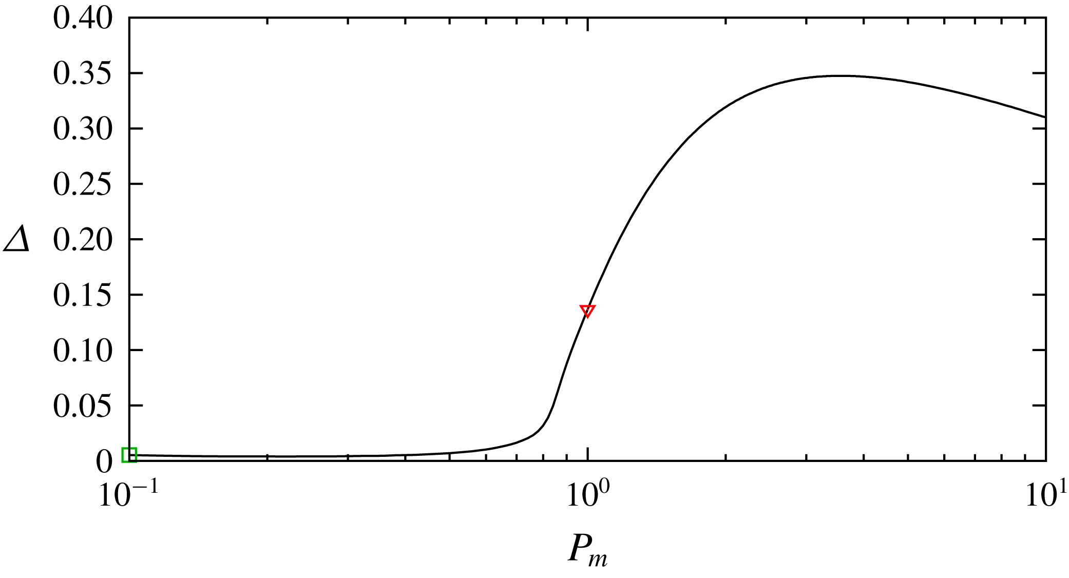
The magnetic Prandtl number dependence of the solutions found at the Chandrasekhar state
 $B_{0}=1$
. Here
 $R=1000$
. The mirror-symmetric mode found for the perfectly conducing conditions is used (the solution at
 $P_{m}=1$
corresponds to the lower triangle on the lower branch of the dashed curve in figure 3).

The numerical results so far have revealed that for
 $P_{m}=1$
the nonlinear solutions continued from small
 $B_{0}$
eventually disappear for large
 $B_{0}$
. For the perfectly insulating case, the solution branch never crosses the Chandrasekhar limit
 $B_{0}=1$
. Solutions can be found at
 $B_{0}=1$
for the perfectly insulating case, but the maximum
 $B_{0}$
that the solution can reach is only slightly greater than unity. This would cast some doubt on the existence of subcritical instability in the sub-Alfvénic regime.
The solution can be found for much larger
 $B_{0}$
when
 $P_{m}$
is large or small. Here we demonstrate this by using the mirror-symmetric mode computed for the perfectly conducting case (the behaviour of the solutions is qualitatively similar for the sinuous mode/perfectly insulating case). We vary
 $P_{m}$
from this solution as shown in figure 6 to see that the nonlinear solution exists for a wide range of
 $P_{m}$
. The starting point of the computation is indicated by the lower triangle, which corresponds to that on the lower branch seen in figure 4. As one can expect from figure 6, the character of the solution is different for
 $P_{m}>1$
and
 $P_{m}<1$
.
With increasing
 $P_{m}$
and
 $B_{0}$
, the solution tends to possess a complicated flow structure similar to that of figure 5(a,b). Some tentative computations for
 $P_{m}=10$
show that along the solution branch the value of
 $B_{0}$
can be increased up to about
 $2$
. However, we do not go into much detail for the range of existence of the solutions in this paper, as our numerical resolution eventually becomes unreliable.
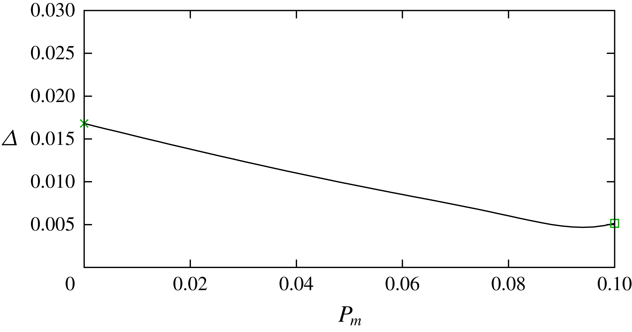
The continuation of the mirror-symmetric mode solution branch towards the inductionless limit
 $P_{m}\rightarrow 0$
. Here
 $R=1000$
. The perfectly conducing conditions are used. The strength of the external magnetic field is changed as
 $B_{0}=1/\sqrt{10P_{m}}$
(the Hartmann number
 $H\approx 316.2$
).

For small
 $P_{m}$
, on the other hand, the structure of the solution remains the relatively simple vortex–Alfvén wave interaction form (see figure 5
c,d) and thus the computation is not too difficult. The smaller the value of
 $P_{m}$
, the greater the value of
 $B_{0}$
we can reach along the solution branch. This is because on decreasing
 $P_{m}$
the Ohmic diffusion term in the induction equations will become significant, and hence a stronger external magnetic field is necessary to support the nonlinear solution. The ultimate behaviour of the solution as
 $P_{m}\rightarrow 0$
and
 $B_{0}\rightarrow \infty$
can be described by the so-called inductionless limit (e.g. Davidson Reference Davidson2001). The limiting result follows by first considering the Hartmann number
 $H=B_{0}RP_{m}^{1/2}$
as a constant. Then assuming the scaled magnetic field
 $\widetilde{\boldsymbol{b}}=P_{m}^{-1/2}\boldsymbol{b}$
, the velocity
 $\boldsymbol{v}$
and the total pressure
 $q$
are all
 $O(P_{m}^{0})$
quantities, the limit of
 $P_{m}\rightarrow 0$
in (2.4) gives the inductionless limit equations
 $$\begin{eqnarray}\displaystyle & \displaystyle (\unicode[STIX]{x2202}_{t}+U_{b}\unicode[STIX]{x2202}_{x}+\boldsymbol{v}\boldsymbol{\cdot }\unicode[STIX]{x1D735}-R^{-1}\unicode[STIX]{x1D6FB}^{2})\boldsymbol{v}-R^{-1}H(U_{b}\unicode[STIX]{x2202}_{x}\widetilde{\boldsymbol{b}}+U_{b}^{\prime }\widetilde{b}\boldsymbol{i})=-\unicode[STIX]{x1D735}q, & \displaystyle\end{eqnarray}$$
 $$\begin{eqnarray}\displaystyle & \displaystyle \unicode[STIX]{x1D6FB}^{2}\widetilde{\boldsymbol{b}}=H(U_{b}^{\prime }v\boldsymbol{i}-U_{b}\unicode[STIX]{x2202}_{x}\boldsymbol{v}), & \displaystyle\end{eqnarray}$$
 $$\begin{eqnarray}\displaystyle & \displaystyle \unicode[STIX]{x1D735}\boldsymbol{\cdot }\boldsymbol{v}=\unicode[STIX]{x1D735}\boldsymbol{\cdot }\widetilde{\boldsymbol{b}}=0, & \displaystyle\end{eqnarray}$$
Figure 7 presents the solution branch continued towards the inductionless limit. The starting point of the computation is the green square at
 $P_{m}=0.1$
, which exactly corresponds to that seen in figure 6. Unlike figure 6, here the value of
 $B_{0}$
is varied as
 $1/\sqrt{10P_{m}}$
so that the Hartmann number becomes a constant. The solution branch indeed reaches very small
 $P_{m}$
, and then the inductionless limit equations (2.4) are used to compute the solution at
 $P_{m}=0$
. Because of the inductionless limit scaling used, the value of
 $B_{0}$
becomes formally infinite there.
The parameter dependence of the inductionless limit is important as it gives the leading-order behaviour of the small
 $P_{m}$
solutions. When
 $R$
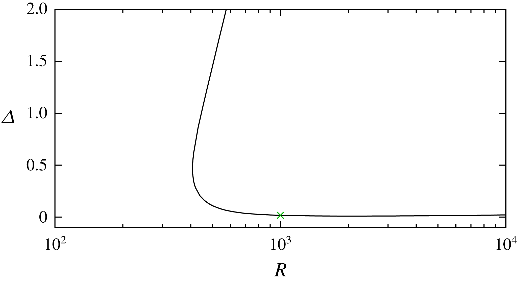
is decreased, the solution branch is expected to have a saddle-node point because the energy analysis gives
 $R_{E}=20.66$
, which is identical to that of the purely hydrodynamic plane Couette flow. Figure 8 shows the bifurcation diagram of the inductionless limit solution found in figure 7; the saddle-node point numerically found is at
 $R=407.4$
. Similar to figure 4, the flow regime of the solutions on the lower branch is found to be of the vortex–Alfvén wave interaction type, while that on the upper branch is not. This means that at least the lower-branch state would persist for asymptotically large Reynolds number; we confirm the existence of the solution by increasing
 $R$
up to 10 000. Thus the result obtained in this section strongly suggests that the subcritical instability exists in a broad range of sub-Alfvénic regime, when
 $P_{m}$
is small.
The bifurcation diagram of the inductionless state found in figure 7 (
 $P_{m}=0$
and the inverse of the magnetic Mach number
 $B_{0}$
is infinite). The mirror-symmetric mode solution is shown for
 $R=1000$
and
 $H\approx 316.2$
. The perfectly conducing conditions are used on the walls.

6 Conclusion
We have theoretically and numerically studied subcritical MHD instabilities by computing finite-amplitude solutions of magnetised plane Couette flow in a wide parameter range of
 $B_{0}$
,
 $P_{m}$
and
 $R$
. Perfectly conducting or insulating conditions are used on the walls. As seen in the purely hydrodynamic studies, we expect that the existence of the steady solutions is strongly correlated with that of subcritical transition to turbulence (Itano & Toh Reference Itano and Toh2001; Hof et al.
Reference Hof, van Doorne, Westerweel, Nieuwstadt, Faisst, Eckhardt, Wedin, Kerswell and Waleffe2004; Skufca et al.
Reference Skufca, Yorke and Eckhardt2006; Wang et al.
Reference Wang, Gibson and Waleffe2007; De Lozar et al.
Reference De Lozar, Melibovsky, Avila and Hof2012).
It was shown in Deguchi (Reference Deguchi2019b
) and § 3 that the nonlinear solutions exist for almost the entire super-Alfvénic regime (
 $B_{0}\in [0,1]$
), if the Reynolds number
 $R$
is not too small. The shear on the walls,
 $\unicode[STIX]{x1D6E5}$
, is monitored to measure the solutions. When
 $\unicode[STIX]{x1D6E5}$
tends to a constant for large
 $R$
, the asymptotic flow structure can be described by the vortex–Alfvén wave interaction theory of Deguchi (Reference Deguchi2019a
).
When
 $P_{m}=1$
, whether the solution branch can be continued to the Chandrasekhar state
 $B_{0}=1$
depends significantly on the conductivity of the walls. From the numerical result using perfectly insulating conditions, it is likely that the solution branch cannot pass through
 $B_{0}=1$
. This may look like a manifestation of Chandrasekhar’s theorem at first glance, although the theorem is deduced assuming the smallness of the perturbation. Curiously, for the perfectly conducting case, numerical solutions are found at the Chandrasekhar limit. This result suggests that for finite-amplitude states, conductivity of the walls acts as a destabilisation mechanism, as opposed to the linear MRI found by Rüdiger et al. (Reference Rüdiger, Schultz, Stefani and Mond2015).
Motivated by those numerical results, in § 4, an extension of the Chandrasekhar theorem to the nonlinear regime was attempted. Using the energy budget equations for Elsässer variables, we found that as long as the assumption (iii) is satisfied and
 $P_{m}=B_{0}=1$
, we can establish stability against the nonlinear and diffusive perturbations. However, the diffusivity affects the stability property in a more complicated manner than that for ideal flows through the boundary terms, and therefore the extended theory cannot work for both perfectly conducting and insulating walls. Nevertheless, we were able to explain the numerical results in § 3, by showing the non-existence of nontrivial solutions in the reduced problem based on the vortex–Alfvén wave interaction theory, when the perfectly insulating conditions are used. The diffusivity is the leading-order effect everywhere for the roll-streak component in the reduced problem, unlike the linear MRI studied by Rüdiger et al. (Reference Rüdiger, Schultz, Stefani and Mond2015). For the perfectly insulating conditions, we can show that there is no energy input to the streak fields (i.e. the
 $x$
component of the mean field) through the boundary. This special property of the flow eventually led us to show that the hydrodynamic and magnetic streak components must take similar form. Thus no wave driving the whole self-sustaining process can be generated because of Chandrasekhar’s theorem for the ideal stability problem of the streak fields. When the walls are perfectly conducting, on the other hand, there may be some energy input through the boundary, and hence the above arguments cannot hold.
In § 5, we showed that the nonlinear solution branch can be continued for large
 $B_{0}$
, when
 $P_{m}$
is small. The solutions at the asymptotic limit
 $P_{m}\rightarrow 0$
can be computed by using the inductionless limit equations. In order to find the limiting solution, the magnetic Mach number is scaled as
 $B_{0}^{-1}\sim O(P_{m}^{1/2})$
. The existence of nonlinear solutions for
 $B_{0}\in [1,\infty )$
is confirmed under this scaling.
In summary, solutions that may be responsible for subcritical transition to MHD turbulence have been found for almost the whole range of
 $B_{0}$
and not too small
 $R$
. Their existence and properties are largely influenced by
 $P_{m}$
and the conductivity of the walls. This paper exemplified a few cases where some theoretical analyses are possible, but our understanding of the subcritical MHD instability is still far from complete. The precise role played by the solutions in subcritical transition to turbulence must be studied using direct numerical simulations in the future. Aside from that obvious issue, there are many problems left open. For example, an interesting question would be whether there is a subcritical instability driven purely by a linear unidirectional magnetic field. The numerical results in this paper suggest a negative conclusion for the existence because solutions cannot be found unless they are subjected to a finite amount of shear. Another issue is that the range of
 $P_{m}$
studied in this paper is rather narrow compared with some real world problems. For typical astrophysical and planetary flows,
 $P_{m}$
is usually very small (e.g. stars, disks) or very large (e.g. galaxies) depending on the object. Thus the
 $P_{m}$
dependence of the solutions in particular for large
 $P_{m}$
would deserve a more careful future study.
The results here may be of interest in the context of energy dissipation in magnetised plasmas such as stellar coronas, where resonant absorption can commonly be found. For certain astrophysical objects such as accretion discs, the effect of the streamline curvature in the base state is known to be important, as it causes a number of linear instability mechanisms such as centrifugal instability and the MRI. Such curvature effects are ignored in the present paper, but the numerical methods used here can be modified to work in cylindrical geometry to study the MHD Taylor–Couette flow. Thus there would undoubtedly be considerable scope for conducting numerical continuation on that flow to study possibly more complex interplay between the various MRIs and the subcritical MHD instability recently found by Guseva et al. (Reference Guseva, Hollerbach, Willis and Avila2017).
Acknowledgements
This work was supported by Australian Research Council Discovery Early Career Researcher Award DE170100171. The author acknowledges the helpful comments of the referees.
Appendix A. Derivation of (4.6)
In order to derive (4.6), we have to show
 $$\begin{eqnarray}\unicode[STIX]{x1D6EC}=-{\mathcal{D}}-R\frac{\text{d}{\mathcal{E}}}{\text{d}t}.\end{eqnarray}$$
We first remark that for the perfectly conducting case,
 ${\mathcal{D}}={\mathcal{E}}=0$
from
 $\unicode[STIX]{x1D6EC}=0$
(see table 1). For the perfectly insulating case, from the
 $y$
component of the induction equations
 $$\begin{eqnarray}\frac{\text{d}\widehat{f}_{m,n}}{\text{d}t}+U_{b}\text{i}m\unicode[STIX]{x1D6FC}\widehat{f}_{m,n}=R^{-1}(\widehat{f}_{m,n}^{\prime \prime }-L\widehat{f}_{m,n})\end{eqnarray}$$
must be satisfied on the walls. Then using (2.9) and (A 2),
 $$\begin{eqnarray}\displaystyle & & \displaystyle \hspace{-30.0pt}2\unicode[STIX]{x1D6EC}=[\overline{\overline{(aa_{y}+bb_{y}+cc_{y})}}]_{-1}^{1}=\mathop{\sum }_{m,n}[L\widehat{f}^{\prime \ast }(L\widehat{f}_{m,n}+\widehat{f}_{m,n}^{\prime \prime })]_{-1}^{1}\nonumber\\ \displaystyle & & \displaystyle \hspace{-30.0pt}\quad =\mathop{\sum }_{m,n}\!\left(\!-2L^{5/2}(|\,\widehat{f}_{m,n}(1)|^{2}+|\,\widehat{f}_{m,n}(-1)|^{2})-RL^{3/2}\frac{\text{d}}{\text{d}t}\!\left\{\frac{|\,\widehat{f}_{m,n}(1)|^{2}+|\widehat{f}_{m,n}(-1)|^{2}}{2}\right\}\!\right)\!.\end{eqnarray}$$
Therefore, comparing this result with (A 1),
 $$\begin{eqnarray}\displaystyle & \displaystyle {\mathcal{D}}=\mathop{\sum }_{m,n}L^{5/2}(|\,\widehat{f}_{m,n}(1)|^{2}+|\,\widehat{f}_{m,n}(-1)|^{2}), & \displaystyle\end{eqnarray}$$
 $$\begin{eqnarray}\displaystyle & \displaystyle {\mathcal{E}}=\mathop{\sum }_{m,n}L^{3/2}\left\{\frac{|\,\widehat{f}_{m,n}(1)|^{2}+|\widehat{f}_{m,n}(-1)|^{2}}{4}\right\}. & \displaystyle\end{eqnarray}$$
Appendix B. Theoretical details of the discussion in § 4.3
Here we show that the wave components cannot maintain the roll-streak components when the streak fields are equipartitioned (i.e.
 $\overline{u}=\overline{a}$
).
When
 $s=0$
, the only possible solution of the streak stability problem is
 $\widetilde{q}=0$
. In the absence of the wave components, the roll components cannot be sustained because there is no energy input. Then
 ${\mathcal{I}}$
in the second streak energy equation (4.14) can be neglected, leading to that the streak components must be zero identically. Therefore, no non-trivial solution is possible.
When
 $s\neq 0$
we have a type 1 interaction. In this case, we use the fact that the equation for
 $E_{-}$
, equation (4.3a
), is now significantly simplified from the complete case. First, the left-hand side of this equation is of course zero, because we are considering equilibrium states. Next, we consider the contribution from the wave components on the right-hand side; here note that the diffusion effect in the thin resonant layer does not contribute to the leading-order interaction problem, as shown by Deguchi (Reference Deguchi2019a
). Since the wave is predominantly ideal, the contribution is negligibly small in the terms originating from the diffusion effects, namely
 $D_{-}$
,
 $\unicode[STIX]{x1D6EC}$
and
 $\unicode[STIX]{x1D706}$
. The other boundary term
 $\unicode[STIX]{x1D6E4}$
vanishes as well because the impermeability condition
 $\widetilde{v}=0$
at
 $y=\pm 1$
also ensures
 $\widetilde{b}=0$
there through the frozen condition (4.13). Finally, the contribution from the roll-streak components must be treated. The boundary terms
 $\unicode[STIX]{x1D6EC},\unicode[STIX]{x1D706}$
are actually zero, because
 $\overline{a}=0$
on the walls. Therefore, we have
 $D_{-}=0$
, from which we can deduce that the hydrodynamic roll components
 $[\overline{v},\overline{w}]$
must vanish identically; this also means that the wave amplitude driving them is zero. Turning back to (4.14), we see that
 $\overline{u}=\overline{a}=0$
because now
 ${\mathcal{I}}=0$
. Thence, we merely have a trivial solution.