1. INTRODUCTION
Layout is the arrangement of elements, usually within a given area for a particular purpose. In the context of architecture and urban design it relates to the arrangement of spatial elements (e.g., parcels, buildings, rooms) on certain scales. Scales denote the different contexts of a design (e.g., urban neighborhood, building volumes, functional areas, floor plans). Jo and Gero (Reference Jo and Gero1998) describe layout as “the assignment of discrete space elements to their corresponding locations while the space elements have relationships among each other.”
The design of layouts is of central importance in architecture and urban design. The arrangement, shape, and proportions of elements have a decisive impact on the quality and sustainability of buildings, neighborhoods, or entire cities. Depending on the project and the context a range of different requirements needs to be met. To meet these requirements, the conventional design process involves making assumptions at the beginning of the process, which are then constantly reviewed and refined. A prerequisite for this is a significant reduction in the complexity of a design problem with the aid of guiding images or principles (Lawson, Reference Lawson2006). These guiding principles, which are set at the highest level of scale or abstraction, then define the framework for design decisions at lower levels of scale. Such procedures are known as top-down strategies, whereby the functional requirements are usually subordinated to the guiding image. The aim of the efforts in the development of computer-based methods for solving layout problems is to assist the designer in complex tasks using bottom-up strategies that make it possible to take into account complex functional criteria on different scales more or less equally.
The creative development of a design task usually takes place independently of the optimization of functional considerations. Conversely, the automated generation of designs using computer-based methods is undertaken without taking account of subjective ideas or creative intentions. A central area of potential for improving computer-aided design processes can be seen in the consideration of both creative design and optimization methods. In this paper we will first clarify which generative methods are suitable for such an approach (Section 2) and the need for interaction in such systems (Section 3). We then present a mechanism for solving layout problems (Section 4) and apply it to hierarchical structured and nonhierarchical structured layout problems. Finally, we review the special characteristics, advantages and disadvantages of both types (Section 5).
2. METHODS FOR THE COMPUTER-BASED GENERATION OF LAYOUTS
The solution of layout problems using computer-based methods is a central issue in the application of artificial intelligence in the field of architecture. Layout problems are usually very complex problems, which need to meet a variety of requirements. The number of solutions increases exponentially with each factor to be considered, for example, the number of rooms (March & Steadman, Reference March and Steadman1971). From the perspective of complexity theory, layout problems fall into the category of so-called nondeterministic polynomial time complete problems.
Since the early 1960s different methods have been developed for the computer-based solution of such problems (Whitehead & Eldars, Reference Whitehead and Eldars1964). Common to all of these methods is a generative mechanism for the production of alternative solutions and an evaluation mechanism to evaluate the variants. The difference we want to take closer look in this section lies in the respective weighting of the two mechanisms.
In terms of design support systems we can distinguish between direct and iterative methods. Direct methods provide an exact solution for a problem within a finite time period. They are usually based on a comprehensive analytical consideration of the problem. Iterative methods, by contrast, usually deliver only approximate solutions to a problem by gradually adapting them to ideal requirements. Another important differentiating factor is the amount of knowledge initially required to obtain useful results. On the one hand, there are methods that require extensive knowledge for the generative mechanism and comparatively little for the evaluation mechanism. This ensures that an appropriate generative system does not deliver useless results to begin with. On the other hand, there are methods that require little knowledge of the problem for the generative mechanism, but require an elaborate evaluation mechanism. Based on the results of the evaluation, useful alternative solutions are improved in an iterative process until they reach a certain quality.
In this context it is important to clarify the difference between problem knowledge and evaluation criteria. Problem knowledge includes a detailed analysis of an actual state as well as a precise specification of the steps to be performed in order to achieve a particular state. Evaluation criteria, however, specify how properties of a solution should be evaluated. Because it is generally easier to expand the evaluation criteria than to adapt a generative mechanism to a new problem, iterative methods that require little problem knowledge are easier to adapt to changing problems than direct methods.
In general, we can state that in approaches that require extensive problem knowledge, the solution of a problem is already largely determined in the specifications, and in procedures that require little problem knowledge, the solution is not explicitly described in the generative mechanism but framed by the evaluation criteria. Approaches that require extensive problem knowledge include logic programming methods (Coyne, 1988), the classic shape grammar method (Stiny & Mitchell, Reference Stiny and Mitchell1978; Duarte, Reference Duarte2000) and the pure constraint-based systems (Li et al., Reference Li, Frazer and Tang2000; Medjdoub & Yannou, Reference Medjdoub and Yannou2001). These methods are particularly suitable for processing well-defined problems, such as the imitation of certain forms based on shape grammars. Approaches that require little problem knowledge include methods such as cellular automata (Batty & Xie, Reference Batty and Xie1994; Coates et al., Reference Coates, Healy, Lamb, Voon, Rossignac and Sillion1996), agent-based systems (Coates & Schmid, Reference Coates and Schmid2000), and evolutionary algorithms (EAs; Hower, Reference Hower1997; Rosenman, Reference Rosenman, Dasgupta and Michalewicz1997; Jo & Gero, Reference Jo and Gero1998). In the following section we examine why from our point of view the latter are more suitable for solving design problems.
2.1. Design problems
In dealing with design support methods, it is necessary to distinguish between operational and nonoperational problems. A problem is operational if it can be described so precisely that one can specify the steps needed to resolve it. The concrete, definable, tangible criteria for describing the problem are called operational criteria. In contrast, nonoperational problems, are “vaguely defined, important elements of the task are unknown or not (quantitatively) definable, their solution criterion is not formulated clearly, the decision process is less concerned with finding solutions, but rather with the specification and differentiation of the problem as well as with the closure of open constraints” (Röpke, Reference Röpke1977). For these problems, there is no clear right or wrong solution. Design problems are usually about nonoperational problems, what distinguishes them from most of the problems of scientific research (Simon, Reference Simon1969). The solution of nonoperational problems always depends on subjective and contextual aspects.
With regard to the aforementioned distinction between methods that require extensive or little problem knowledge one can add that, although both approaches require operational criteria, the latter does not have to include a complete analysis of the complex problem. Generally it is sufficient to specify heuristics that provide reasonable assumptions for solving a problem but do not guarantee a solution. The fact that a problem solution cannot be guaranteed means that the method employed will make mistakes in the search for solutions. At best, these errors can be used productively to identify new, unexpected solutions. Such system characteristics open the possibility of finding creative solutions to problems, which computer systems at present are not very capable of.
2.2. Evolutionary algorithms
A solution can be called creative when it is not apparent from a detailed description of the problem. This situation illustrates why direct methods, which require extensive problem knowledge are not suitable for supporting creative processes. EAs are so-called heuristic methods that do not guarantee the solution of a problem in any particular case, but considerably reduce the time required to solve the problem. Of course, EA, like all computer programs, only function if all the individual steps to be performed are defined. Compared with other algorithms, however, they require very little problem knowledge. Stochastic processes thereby ensure a certain range of possible variants, which can lead to surprising results.
When solving design problems we are usually dealing with several contradictory requirements. A good solution for such multicriteria problems is always a compromise in the form of a balanced account of the various requirements. In the field of computer-based optimization problems such problems are called multiobjective optimization problems (MOOP). EA have the potential to find all the possible compromise solutions, which are known as pareto-optimal or nondominated solutions (Deb, Reference Deb2001; Coello et al., Reference Coello, Lamont and Veldhuizen2007).
2.3. Interactive systems
Even with EAs there is still the problem that certain requirements, such as the definition of the objective functions (operational criteria) for a design problem, need to be specified explicitly. A common approach for the input of these criteria is to integrate the user. The importance of interactivity in design support systems has already been emphasized in several similar projects such as in Weinzapfel et al. (Reference Weinzapfel, Johnson and Perkins1971), Ruch (Reference Ruch1978), Michalek and Papalambros (Reference Michalek and Papalambros2002), Arvin and House (Reference Arvin and House2002), and Elezkurtaj (Reference Elezkurtaj2004). The aim when developing interactive systems is to achieve an interplay between the generative system and the subjective ideas of the user.
With regard to the aforementioned distinction between direct and iterative process, one can note that interaction with direct systems is limited to changing initial values and running calculations after each change. With iterative systems, by contrast, interventions during the generative process are permitted, either by changing the rules of the generative mechanism or the evaluation criteria.
3. THE REQUIREMENTS OF AN INTERACTIVE DESIGN SYSTEM
Although operational problems are usually straightforward to solve algorithmically, nonoperational problems depend on the interpretation of a problem by a human. The integration of human capabilities is necessary to reduce certain aspects of the design process to operational problems. Because “all that is possible is the conversion of particular problems from ill-structured to well-structured via the one transducer that exists, namely, man” (Ernst & Newell, Reference Ernst and Newell1969, p. 363). Requirements for adequately integrating human capabilities into a generative design system have been discussed in Schneider et al. (Reference Schneider, Fischer and König2010). These requirements are clarified and extended by the following four desirable system properties:
1. Adaptive: A generative system should allow the definition of new constraints/requirements for a problem at any point in time because designing is not simply searching a solution space but also its continual adjustment. This process of ongoing adjustment does not follow a predefined scheme. Adaptive therefore means that the problem definition can be defined by the users themselves and changed during the problem solving process. A prerequisite for such an adaptive system is circularity.
2. Iterative: Designing is an iterative process that brings forth new problems. Once a solution is found new problems emerge that need to be addressed in further iterations. To solve these new problems, it may be necessary to discard old solutions, which can lead to complex dependencies between different solutions. Design problems are therefore not clearly definable in advance but gradually emerge during the design process. Unlike “presented problem situations” one has to deal with “discovered problem situations” (Getzel & Csikszentmihalyi, 1967).
3. Exploratory: Where contradictory criteria are involved, it is important that a generative system offers a broad range of equivalent compromise solutions. This means that the system offers solutions that are distributed as evenly as possible across the so-called Pareto front (which contains all compromise solutions). This ensures that all relevant solutions are provided. The choice between the compromises must be made by a user unless no additional criteria are introduced.
4. Immediacy: The impact of changes to the generative rules and evaluation criteria should be visible as quickly as possible, that is, ideally in a fraction of a second. Immediacy makes it possible to understand the connection between cause and effect during the search process. In this context it is important to choose a suitable representation for the solution variants to facilitate rapid appraisal of the relevant properties of a variant. In general, this should be done in a graphical or diagrammatic way. User interaction is most successfully realized through graphic representation and not separately via text-based parameters.
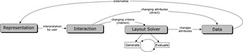
To consider these properties, it is important to carefully coordinate the various aspects of the layout system. These aspects relate to the graphical representation, user interaction, the layout solver, and management of data. The interplay of these aspects can be considered as a circular process, where interventions at each level have a direct impact on the overall system (see Fig. 1).
Partial aspects of the interactive layout system (Schneider et al., Reference Schneider, Fischer and König2010).

In the following section we concentrate on the description of the layout solver and then, based on this solution mechanism, examine two different types of layout problems (hierarchical and nonhierarchical layout) and discuss their properties within the interactive layout system.
4. LAYOUT SOLVER
In this section we present a mechanism for solving layout problems with the aim of generating layout solutions as quickly as possible. For the user interaction, high computational speed is especially important so that the effects of changes are immediately visible (see point 4 in the previous section). To this end, an additive method is used, which first produces a dense packing of the elements considered, and secondly ensures the topological relations between the elements. For the elements we use rectangles.
4.1. Dense packing
The problem of dense packing occurs when a certain number of spatial elements need to be arranged within a given area without overlapping and with as few gaps as possible. The elements and the bounding area can have fixed values, as, for example, in the case of packing cargo boxes in a truck. In architectural layout design, both the elements to be packed (the rooms) and the surrounding area (the building) can vary within certain limits. In the test scenario discussed in this section, we assume a fixed building outline and deal with the two-dimensional packing of individual rooms that are flexible in their dimensions, within defined minimum and maximum limits, but always have to respect a given area. The sum of the areas to the elements corresponds to the area of the building outline.
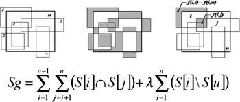
The problem to be solved was described formally by Elezkurtaj and Frank (Reference Elezkurtaj and Franck2001, Reference Elezkurtaj and Franck2002) as follows (Fig. 2): minimize the sum of all intersection areas S g. This is calculated as the sum of the intersection areas of all elements (S i\S j) and the weighted sum of the intersection areas arising from the overlapping of the elements with the surrounding area (S i\S u).
A graphical and formal representation of the calculation of the total intersection areas by Elezkurtaj and Franck (Reference Elezkurtaj and Franck2001).

The restriction that rectangles may not extend beyond the limits of the surrounding area, as shown in Figure 2, can be integrated in the calculation of S g and used for the minimization of S g. As an alternative to this method overlaps with the bounding rectangle can be avoided in advance by immediately shifting any rectangles that overlap the bounding box within the boundary so that no overlap occurs. This alternative simplifies the calculation of S g to

where t indicates the number of the iteration.
4.1.1. Collision detection
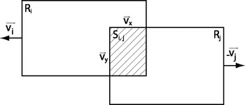
For the algorithmic solution of the problem illustrated in Figure 2, the process of collision detection between two geometric elements (rectangles) is useful in order to reduce their degree of overlap by mutually repelling the elements. If two rectangles intersect, as shown in Figure 3, the smallest rebounding vector (v x or v y) is chosen, so that each rectangle can be shifted by half of this vector in different directions (v i and v j).
The calculation of the rebound vectors of two overlapping rectangles.

The rebounding of the rectangles is an efficient method for reducing the sum of all intersection areas S g. With this method only the positions of the rectangles are adjusted (location change). For an overlap-free packing of rectangles (S g = 0) it is usually also necessary to change the proportions, that is, length and width, of the rectangles.
For the adjustment of the proportions the same method can be used as used for the rebounding of the rectangles. The only difference is that in this case, the vectors are not used to move the rooms, but to change the width or height of the rectangles. In the example in Figure 3, the width of R i would be reduced by the amount of the vector v i, while simultaneously increasing the height. Thus, the area F i remains constant, despite the change of proportions. The same is done with the second rectangle Rj.
For the implementation of the previously described procedure the following additional operators are introduced: the factor β for weighting the rebound vectors, the probability ρL of executing the rebound function when two rectangles overlap, the factor α for weighting the proportion change vectors and ρG, which describes the probability of executing the proportion change function. To summarize, we can represent the two functions for the adjustment of the rectangles as follows:
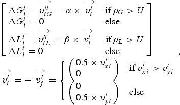
where ΔG i specifies the proportion change and ΔL i specifies the localization change at the iteration step t and U is a uniformly distributed random number on the interval [0, 1], which is redrawn at every call.
Because the collision process itself does not serve as a satisfactory solution algorithm for dense packing, the following section introduces the technique of evolutionary strategy (ES) and demonstrates how collision detection can be combined with an ES.
4.1.2. Evolutionary strategy
The simplest form of the ES is the so-called two-tier (1 + 1)-ES (Rechenberg, Reference Rechenberg1994). (µ + λ)-ES represents the general notation for an ES with a (+)-selection, where µ displays the number of parents and λ the number of children in a population P. (+)-Selection means that for the next generation the parents remains unchanged and are selected together with the children. As a result, good solutions will not be lost through mutation or crossover, but can be replaced only by better solutions. The (+)-selection is relative continuous because there are no abrupt changes between different solutions. With the (,)-selection, by contrast, the pool for the next generation is only selected from the children. This can lead to a degradation of the fitness values because the best individuals may be changed by mutation and recombination. The advantage of the (,)-selection is that the ES does not get stuck so easily in local optima and can adapt better to changing targets.
The quality of an individual is calculated on the basis of the evaluation function f. From λ individuals µ individuals with the highest quality are taken to the next generation while the others are deleted. The evaluation function used in our case is the function for the calculation of S g given in formula (1). The smaller S g is, the higher the quality of an individual.
In the simplest form of an ES, an individual a k with the index k includes with the specific set of object parameters X k and an evaluation function f (Xk):

A specific object parameter Xk for an individual a k, in turn, includes the parameters of a single element Xk = {X 1, X 2, … , X i}. Here, X i is also referred to as a gene that encodes the x and y position (px and py), height h and breadth b of a rectangle:

The iterative scheme of the ES can be applied to this set of parameters. The mutation operations, which are used to randomly change the object parameters, are specified with

The parameter h i is calculated automatically after changing b i to fulfill the condition of keeping the area F i of the rectangle constant: h i = F i/b i.
For the ES, the functions for changing the proportion and location (2) are used as mutation operators. To allow purely random changes, further mutation operators are introduced that cause a random change in the position or proportion with a probability of ρZ:
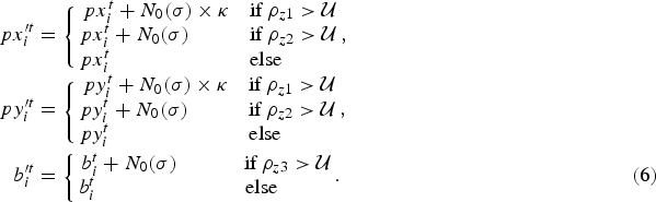
N 0 denotes a normal distributed random number; the factor κ allows greater changes.
Because of the combination of specific proportion and localization changes (2) and purely random changes, the method developed so far can be termed a hybrid algorithm or hybrid ES.
4.1.3. Hybrid (µ + λ)-ES with recombination operators
When using several parents per generation µ > 1, ρ parents can be involved in the production of a child. Accordingly the notation of an ES is supplemented by the parameter ρ: (µ/ρ + λ)-ES. For our purposes, we consider the discrete recombination (Bäck et al., Reference Bäck, Hoffmeister and Schwefel1991) in which each object parameter is randomly chosen from one of the ρ parents (Deb, Reference Deb2001, p. 137; ρ = 3):
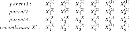
Furthermore, the recombination operator r is introduced. For ρ = 2, the recombination of two individuals can be described as follows:

where X b and X c represent two randomly selected parents selected via the recombination operator r.
At this point it is important to realize that, as noted in (4) above, a gene X i includes the complete set of properties of a rectangle, which should not be destroyed by recombination. This fact is relevant because we do not want to change predefined area of a rectangle. If we were to subject the properties of the rectangles to recombination, new rectangles would arise as a result of new values for heights and widths, which would necessarily entail new surface areas. If the surface area is allowed to vary, the population would rapidly be dominated by small elements because they cause fewer overlaps. The sum of the area of the rectangles must therefore always be equal to the area of the surrounding rectangle.
After (8), the vectors X i of two parents are randomly combined for the generation of X i′. Here, U denotes a uniformly distributed random number on the interval [0, 1], which is redrawn on every call. The recombination operator is not used for the production of every child, but only according to a certain probability ρr. The best system properties, that is, the best possible continuous improvement of solutions along with a fast response to changing conditions can be achieved by using a (+)-selection, where the parents can be mutated but to a lesser extent than their children.
Before we look at methods for taking into account topological relationships, the algorithm developed so far (referred to as standard ES) can be summarized as follows:
Step 1. Initialize a population P with µ individuals.
Step 2. Create λ children by
Step 3. Select the µ best individuals from parent and children population for the next generation of parents.
Step 4. If the termination criterion is met, terminate the algorithm otherwise go to step 2.
4.2. Topological relations
Topological relation refers to the adjacency of individual rooms. Two rooms are adjacent to each other when there is no distance between them and they touch on one edge each for a certain length. If we interpret a layout as a plan with individual rooms, this requirement should ensure a minimal passage between two rooms. We consider only cases in which rooms are adjacent to each other or not. Other restrictions that specify, for example, how close a room should be to another or that two rooms should be as far apart as possible are not considered here. In the authors' opinion, such an inclusion makes little sense as in the user's perception two mutually adjacent spaces may occur relatively distant from each other when there is no connection (passage) between them.
Formally, the topological constraint can be expressed as follows:

For the calculation of the function f the distance d between two rectangles with the indices i and j and the contact lengths c of the rectangles are added. To create the desired topological relationships, the objective function f 2 needs to be minimized.
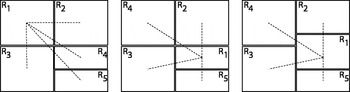
In this section we will examine three ways to achieve the required topological relationships. In the first, the proportions of the rooms are changed (Fig. 4, right), in the second, the spaces are interchanged (permutation; Fig. 4, center) and in the third virtual springs are drawn between rectangles with an existing topological relationship.
Successive approximations of the required topological relations (dashed lines) by permutation (see left and center layout configuration) and proportion change (see center and right layout configuration). The representation does not consider the consistency of the surface area of the individual rooms.

The function for changing proportions of the rooms has already been expressed with the equation ΔG i (2) and needs no further detailing.
4.2.1. Permutation
To achieve a topological relation between elements, one possible method is to exchange elements. The interchange of elements and the consequent change in their arrangement is called a permutation.
Each room or each gene X has an index i. Using this index, particular functions can be allocated to each room and the topological relationships can be defined. When using the recombination and mutation operators, we must now ensure that an individual who represents a layout solution has only one particular index for one particular room. For recombination this requirement is ensured using the “partially mapped crossover” method developed by Goldberg and Lingle (Reference Goldberg and Lingle1985). The mutation of an individual, either swaps two genes with one another, or a randomly chosen gene order is inverted.
4.2.2. Attractions using virtual springs
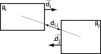
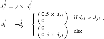
The calculation of the attraction vectors between two adjacent rectangles is done by means of virtual springs between these rectangles (Arvin & House, Reference Arvin and House2002). Their tension is calculated in a similar way to the repelling vectors in Section 4.1.1. First, the distance d i,j between the two rectangles is established (Fig. 5). If d i,j > 0, that is, they are not directly adjacent, the x or y vector component is checked to see which is greater (10). The attraction of the two rectangles occurs in the direction of the larger vector component. Consequently, the resulting attraction vectors either follow the x or y direction, so that the rectangles only move perpendicular to each other.
The greatest difficulty now is to combine all the methods presented so far in such a way that several objective functions can be optimized simultaneously. How this issue can be handled is explained in the next section.
The calculation of the attraction vectors of two rectangles that are adjacent to each other.

4.2.3. Multiobjective optimization problem
With the introduction of topological relationships as a further restriction, we now have two objective functions f 1 (1) and f 2 (9), which both need to be optimized by the layout system. We are therefore dealing with a MOOP (see Section 2.2). These problems are distinguished into conflicting and nonconflicting objective functions. With conflicting objectives not every criterion can be fulfilled completely; the best that is possible is a compromise. For such a compromise, there are usually many different variants that are described as pareto-optimal. A Pareto-optimal state is characterized by the fact that it is not possible to improve a solution without simultaneously degrading another. In the case of nonconflicting objective functions, each criterion can be fully met. In the two objective functions f 1 and f 2 we are usually dealing with nonconflicting objective functions. This is valid as long as we do not stipulate a topological configuration for f 2, for which there is no overlap-free layout of the elements for f 1.
The classical method of solving a MOOP is to reduce it to simple optimization problems by combining all the criteria into one combined criterion (Deb, Reference Deb2001, pp. 13 and 46). For the reduction to one criterion, there are several methods of which the weighted sum is the most common and easiest to implement. Because of the difficulties associated with classical methods, such as the problem of weighting each criterion (Deb, Reference Deb2001, pp. 49–80), these were not used in this case for the MOOP. Rather, we examine an approach to solving the MOOP by combining the vector evaluated genetic algorithm (VEGA) after Schaffer (Reference Schaffer1985) and the vector-optimized evolution strategy after Kursawe (Reference Kursawe1990). The two basic methods are described in detail in Deb (Reference Deb2001, pp. 179–189). To differentiate this from other methods, we refer to the proposed technique as Layout-MOES or L-MOES.
In the context of the present problem, ES for MOOP based on the concept of nondominated solutions, such as the Pareto Envelope-Based Selection Algorithm (Corne et al., Reference Corne, Knowles and Martin2000), have not shown any improvement in system performance. This was mainly due to the choice of selecting the best solutions so far (nondominated set) as the parent population (elite-preserving). This property has led to difficulties in overcoming the local pareto front.
For the EA we use the (µ/ρ + λ)-ES, as defined in Section 4.1.3. The significant extension of the standard ES in this instance is how individuals are selected for the next generation. We still create λ recombined and mutated children from µ parents. Afterward, parents and children are selected together by (+)-selection. For this we calculate two fitness values for each of the two objective functions f 1 and f 2 for each individual. Then the child population is sorted according to the first objective function. A certain percentage of individuals is selected for the next generation of parents. Similarly, we proceed for the second objective function. Relation V = (f 1/f 2) defines the number of individuals selected for the two objective functions f 1 and f 2. During the initialization of V = (µ*0.1/µ*0.9) was chosen. This means, for example, for µ = 10 that only one individual is selected for the minimum overlapping area and nine are selected for the minimum distance. For lower values of µ at least one individual is selected for f 1. If the number of individuals selected for f 1 is increased from the beginning, the system converges more easily at a local pareto front, which approximately corresponds to a local optimum of optimization problems with only one criterion.
Once a layout has been found that exhibits after f 2 a very small distance sum, we introduce a threshold ΨV for changing the ratio V in order to minimize its overlapping areas as soon as possible. It has proven effective to alter the threshold as soon as the individual with the lowest value for f 1 (overlapping areas) falls below a value for f 2 (distances) that is less than twice the number of rooms N R:

The definition of the threshold by the number of rooms works well in the test system, but has to be changed with the scale of the system. We use a similar rule for the selection method. As long as a parent individual a has a value for f 2, which is greater than the threshold ΨV, a (,)-selection is applied, otherwise a (+)-selection is applied with collision detection and random movement of parents, which we already introduced in the standard-ES:

To summarize, the algorithm for the L-MOES can be specified as the following:
Step 1. Initialize a population P with µ individuals.
Step 2. Create λ children by
a. only for (+) selection, see (12): mutation of the parents [purely random mutations (6) and collision detection (2)]
b. Recombination of ρ parents to produce the children [(7)–(8) ρr = 0.75]
c. Mutation of the children (recombinants) [using (6) and (2), permutation (see Section 4.2.1) and virtual springs (10)].
Step 3. Select after (3) and (9), the µ best individuals according to the rules (11) and (12) for the next generation of parents.
Step 4. If the termination criterion is met, terminate the algorithm otherwise go to step 2.
5. HIERARCHICAL STRUCTURED LAYOUT PROBLEMS
In the following, the layout solver presented above is applied to two different types of layout problems. A distinction is drawn between hierarchical and nonhierarchical layout problems. It is shown that for hierarchical layout problems, it is necessary to define relations across hierarchical boundaries. Finally, the advantages and disadvantages for the calculation of both types of layout problems are discussed.
5.1. Hierarchical structuring of elements and the need for cross-border relations
In the previous sections we dealt with the arrangement of elements on a certain level of scale under the premise of ensuring their topological relations. This type of layout problem is referred to as a simply structured or nonhierarchical structured layout problem (NHLP). Another approach lies in the hierarchical structuring of a layout problem (HLP). A layout is termed hierarchically structured when its elements are nested into each other several times. This means that elements can be located within other elements and itself be part of other elements. As an example of an HLP, we can consider a residential building where the corridor and several apartments are arranged on one floor. Within each of the flats, several rooms have to be accommodated and inside these rooms the furniture needs to be arranged. It is worth noting, that the means of hierarchical structuring depends on the situation and can be defined freely by the designer. It is possible to describe a house either as single apartments, or to structure it in certain zones (such as private and public). The concept of HLP was also considered by Flemming et al. (Reference Flemming, Baykan, Coyne, Fox and Gero1992, p. 20), among others.
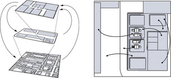
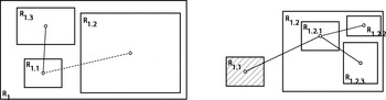
With regard to the relations between the elements, for HLP it is necessary to establish cross-border relations. Cross-border designates the crossing of hierarchical levels or boundaries. Relations refer to the topological relations, which were described in Section 4.2. The need for cross-border relations is obvious since, as shown in Figure 6, elements of one hierarchical level may have relations with elements outside the level. For example, in a residential house, a cross-border relationship is required to connect the corridor of the apartment with the corridor of the house. Consequently, cross-border relations are indispensable for adequately describing layout problems with hierarchically nested elements.
The hierarchical structure (left) and cross-border relations (right).

Thus, on the one hand, HLPs include nested elements. On the other hand, they can include relationships between elements that are located on different levels of hierarchy. The extent to which HLPs with cross-border relations can be solved with the layout solver and what needs to be considered will be clarified below.
5.2. Explicit and implicit internal and external relations
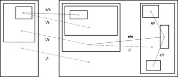
Considering the interaction of a user with the layout system we can distinguish between explicit and implicit requirements (constraints) for a layout. Explicit requirements are requirements that a user explicitly specifies via inputs. Implicit requirements however are requirements that result from the explicit requirements and were not explicitly defined. In the example of defining topological relations in a HLP, this becomes obvious: if two rooms are linked together, there are basically two different types of relations: internal and external. Internal relations are relations of elements within a certain hierarchy level, such as the topological relationship of rooms within an apartment. External relations are relations of elements from different hierarchical levels, for example, the relation of a corridor in an apartment to the access hallway of the building in which the apartment is located. In this case, the apartment and the house's access hallway lie on the same hierarchical level, but the house hallway and the apartment's corridor lie on different levels. This means that the house's access hallway must be adjacent to both: to the corridor of the apartment and to the apartment itself. Because the spatial relation house access hallway–corridor was not explicitly given, this means that this relation has to be created implicitly by linking the apartment corridor with the house's access hallway. In a HLP, two different types of relations exist: internal and external. Relations between elements on the same hierarchical level are called internal; relations between elements on different hierarchical levels are called external. Both internal and external relations can be explicitly specified (by the user). Implicit relations arise only indirectly through the specification of external relations. Here, both internal implicit, as well as external implicit relations, which arise in deeply nested layout problems, can occur (see Fig. 7).
Different types of relations in a problem description of hierarchical structuring of a layout problem; e/i, explicit-internal; e/e, explicit-external; i/i, implicit-internal; i/e, implicit-external.

If the layout solver presented in Section 4 is applied to HLPs, various cases have to be considered. For layout problems where there are only internal relations, the mechanism is readily applicable. For layout problems in which external relationships are present, these must be treated differently. The previously established distinction between implicit and explicit relations is solely important for the user interaction because the user only considers the explicit requirements he or she stipulates. The subsequent automatically created implicit requirements are invisible to the user. The layout solver treats implicit and explicit requirements equally.
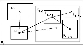
To better understand these special cases, it helps to clarify the procedure of the layout solvers when solving HLPs. Once an element contains other elements, the solver tries to arrange the subelements within the superior element. If there is more than one superior element, these are considered simultaneously. Several optimization processes then run in parallel. The HLP is divided into several NHLP. By way of example, this is shown in Figure 8 and Figure 9. The complex problem in Figure 8 is divided in into two problems (Fig. 9): the arrangement of R 1.1, R 1.2, and R 1.3 in R 1 and the arrangement of R 1.2.1, R 1.2.2, and R 1.2.3 in R 1.2.
The implicit and explicit relations in a simple hierarchical structuring of a layout problem.

Different kinds of relations connecting different level hierarchies for (left) the partial problem R 1 and (right) the partial problem R 1.2.

With regard to achieving dense packing (see Section 4.1), both problems shown in Figure 9 (R 1 and R 1.2) are solvable separately. The creation of dense packing in R 1 can take place independently of the one in R 1.2, because for the subelements R 1.2.1, R 1.2.2, and R 1.2.3 it only means that the height h and width w of the surrounding area R 1.2 can change while packing.
When considering the topological relations, we have to distinguish between internal and external relations. Although internal relations are treated as described in Section 4.2, external relations must be considered separately. First, it is important that external relations impact in only one direction, from the deeper to the higher hierarchical level. On the one hand, this is related to the fact that an implicit link (from R 1.1 and R 1.2) already ensures the requirement for corresponding external adjacency (of R 1.1 and R 1.2.1). On the other hand, potential feedbacks between the subproblems are avoided by considering only one direction. For the solution of R 1 the topological relations between R 1.1 and R 1.2, and R 1.1 and R 1.3 have to be taken into account. For solving R 1.2, however, it is also necessary to consider the external relation to R 1.1 in addition to the internal relations. During the solution of R 1.2 the external element R 1.1 is locked for changes in location and size. The changes to R 1.1 take place in R 1. The solver for R 1.2 treats R 1.1 passively, trying to place the item R 1.2.1 as close as possible to R 1.1.
For the calculation of the distance between the elements that are connected by an external relation, the sum of the distances of the parent element to the external elements needs to be subtracted from the sum of the all the considered distances. In our example, this means that for the calculation of the distance between R 1.2.1 and R 1.1, the distance between R 1.2 and R 1.1 needs to be subtracted.
5.3. Performance comparison of HLP versus NHLP
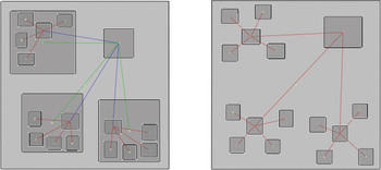
In this section HLP and NHLP are compared with each other in terms of their properties when solving a given test scenario. This scenario consists of generating a layout for a residential building with three apartments (Fig. 10). For the formulation of an HLP, the first level of the hierarchy involves the arrangement of three apartments and one hallway. On the second level, the individual rooms need to be arranged within each apartment. The internal relations on the hierarchical level of each apartment are shaped radially. The corridor within in each apartment has an external relation to the hallway of the house. These external relations generate implicit internal relations from the apartments to the corridor of the building (Fig. 10, left). The formulation of the NHLP consists in the arrangement of individual elements for the rooms of the flats and the house corridor to a single level. Consequently, only internal relations are required (Fig. 10, right).
A schematic representation of the test scenarios each with 16 rooms: (left) hierarchical structuring of a layout problem and (right) nonhierarchical structuring of a layout problem. Red lines are internal relationships, blue lines are external relationships, and green lines are implicit relationships. [A color version of this figure can be viewed online at http://journals.cambridge.org/aie]

The focus of the comparison between the two test scenarios (HLP vs. NHLP) lies on the speed of convergence through which the system finds a useful solution. This is crucial to ensure good user interaction with the system. For a definition of what can be understood as a useful layout solution, the fitness values for f 1 (overlapping areas) and f 2 (distances) are normalized to the interval [0, 1]. This normalization is carried out by assuming maximum values for f 1 and f 2 that lead to a scaling of the fitness values, which primarily covers the value range of useful solutions. For the following analysis and the diagrams in Figure 11 the following scaling functions were used:

where b p and h p specify the breadth and height of the superior rectangle and N rel describes the number of relations in a layout problem. Based on this normalization it is now possible to specify that the layout solutions can be described as useful when the corresponding fitness values fall below certain values:
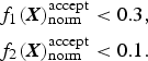
The speed of convergence with which the system provides useful solutions, is counted in generations t of the L-MOES. For rapid user interaction values in (14) should be reached after t = 20 generations [on a computer with average performance (2.4 GHz) this requires ~5 s]. The system should respond with roughly the same speed to interactions by a user, which can be interpreted as interferences to a once optimized layout.
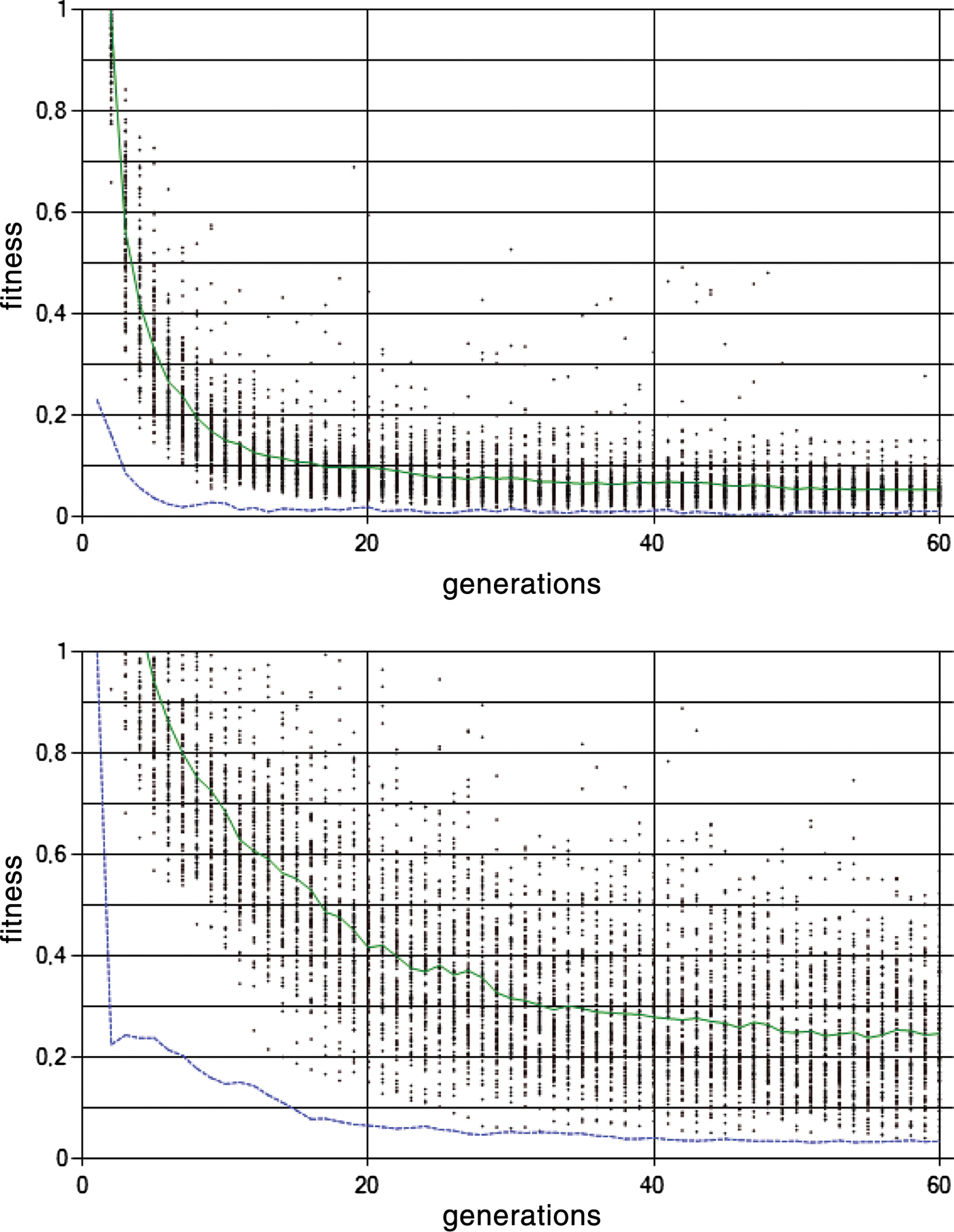
Analysis diagrams for the generation of layouts via L-MOES after 100 runs of the program, each with t = 60 generations. The green solid line represents the average values for f 1, and the blue dotted line represents the mean values for f 2. The diagrams show the analysis of the (top) hierarchical structuring of a layout problem and (bottom) that of the nonhierarchical structuring of a layout problem. The system was initialized with the corresponding scenario from Figure 10. [A color version of this figure can be viewed online at http://journals.cambridge.org/aie]

With the definitions made so far we can now analyze the diagrams in Figure 11. The diagrams represent measurements that were collected during 100 repetitions of the layout system based on the two test scenarios in Figure 10. In both graphs in Figure 11 the data points indicate the fitness values for f 1 (overlap) of each individual run. The green solid line represents the average values for f 1, and the blue dotted line represents the mean values for f 2 after 100 runs.
Comparing the two diagrams in Figure 11 it can be seen that in HLP (left diagram) the mean curve for both f 1 and f 2 falls steeply and reaches lower levels. According to the previous definitions, this means that by using HLP good solutions can be generated in an acceptable speed for appropriate user interaction. In contrast, the two mean curves for NHLP (Fig. 11, right diagram) are much flatter and do not at any time reach values as low as those for HLP. Furthermore, viable solutions are only found for f 1 after an average of about t = 40 generations, which is too slow for responsive user interaction. In addition, the distribution of data points exhibits a much wider spread in NHLPs, which indicates that the system often finds no viable solutions in the considered range of generations. In both diagrams in Figure 11, the average curve for f 2 (distances) returns good results quickly, which can be traced back to rules (11) and (12) of the L-MOES, which first prefer the optimization of f 2.
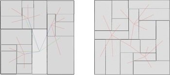
To give an idea of the layout results that lies behind the diagrammatic representation in Figure 11, Figure 12 shows geometric solutions for an HLP (left) and NHLP (right). The effects of the use of different strategies are shown by the fact that in the HLP (left), the apartments are organized within the parent rectangles that were inserted by applying a hierarchy to the problem. In contrast, in the NHLP the rooms are not attached to superior boundaries, resulting in a spatial entanglement of the three apartments.
Typical solutions in the calculation of (left) a hierarchical structuring of a layout problem and (right) a nonhierarchical structuring of a layout problem via L-MOES after t = 60 generations. The corresponding fitness values of both solutions fall below the thresholds defined in (14); accordingly both solutions are defined as useful. [A color version of this figure can be viewed online at http://journals.cambridge.org/aie]

Finally, the advantages and the disadvantages of the compared strategies (NHLP and HLP) can be summarized as follows. The main weakness of NHLPs lies in the slow generation of viable solutions. This is especially problematic when a large amount of elements with many relations needs to be arranged. The main advantage of NHLP is that there is no prior hierarchy applied to the elements, resulting in solutions that remain unaffected by certain conventions, which are otherwise given in the indication of hierarchies. In the example shown, such a convention represents the grouping of rooms of an apartment within a rectangular superior element (Fig. 12).
With regard to the interactive layout system presented in this paper, the usage of HLPs delivers two significant advantages. First, in terms of user interaction the use of hierarchies provides a better overview of the elements to be arranged. This is advantageous because a user can usually only consider a limited number of elements simultaneously (Miller, Reference Miller1956). Second, complex problems with many elements and relationships are solved much faster compared with NHLPs. A disadvantage is that because of the a priori definition of hierarchies, certain solutions are excluded which compromises the requirement in Section 3 that a system should be as exploratory as possible. Consequently, the spectrum of equivalent compromise solutions in HLP is restricted by reducing the search and solution space. The smaller search space also partially explains the higher speed of convergence in HLPs.
It was mentioned in Section 5.1 that the idea of HLPs is not new. For example Coyne and Flemming (Reference Coyne, Flemming and Gero1990) presented it in the ABLOOS framework for layout design. ABLOOS is a hierarchical extension of a system called LOOS (Flemming, Reference Flemming1989), which introduces orthogonal structures for the representation of loosely packed arrangements of rectangles. Although these systems use a different generative mechanism, we can approximately compare their performance with the system presented in this paper.
Flemming et al. (Reference Flemming, Baykan, Coyne, Fox and Gero1992, p. 18) evaluate the performance of the LOOS system. It generates 26 solutions for a test problem with 8 rooms and 11 topological relations in 188 s. Of course, this system would perform faster on current computers, but there is reason to doubt that the generation time for a more complex problem similar to that presented in Section 5.3 (Fig. 10) with 16 rooms and 15 topological relations, would be faster than 5 s, because LOOS calculates all possible solutions using its hierarchical generate and test method. The L-MOES presented in Section 4.2.3 needs approximately 5 s to generate one solution for a given problem. Although the generation of only one solution may be considered as a disadvantage in other contexts, for the requirements of interaction time it can be regarded as suitable strategy.
Harada et al. (Reference Harada, Witkin and Baraff1995) have shown a method for fluid user interaction with discrete constrained layout problems (LOOS can be classified in this category). They trigger a local discrete search, during which certain transformations may be performed. The transition to a new state is visualized using animated visual effects. Such techniques show, that one can also use other generative mechanisms to create a layout system with appropriate user interaction. The advantage of the L-MOES presented here is that it works with continuous parameters that can be manipulated directly by the user, so we do not need further techniques to achieve proper user interaction.
6. CONCLUSION AND OUTLOOK
The present work was developed within a research project that deals with computer-based design methods to support the creative design process. The project aims to develop a system to solve layout problems in architecture, which quickly provides viable results without initially requiring extensive problem knowledge. By gradually adding problem knowledge (in the form of constraints) these results can be elaborated interactively. This approach is contrary to those that require extensive problem knowledge at the very beginning of the solving process and are thereby less able to adapt to constantly changing requirements during the design process.
To solve layout problems, an iterative approach based on EAs was chosen. The method ensures a nonoverlapping arrangement of elements and their topological relationships. Afterward the hierarchical structuring for describing layout problems was discussed. This type of layout description was compared with a nonhierarchical description. Their advantages and disadvantages with regard to the interactive layout system were discussed. It was shown that HLP delivers good results with regard to the speed of convergence. The system is capable of finding viable solutions, even in complex problems after a reasonable time.
In this study we have used an abstract test scenario with a configuration of rectangles to focus on the basic functionality of the system presented. The results shown in Figure 12 can be considered as first design sketches, for example, for the layout of a residential building. Of course, some important aspects are missing, for example, the proportions of rooms need to be considered, the orientation of the rooms in certain directions has to be defined, and the placement of windows needs to be added. From our point of view, however, these are comparatively small problems that can be solved relatively easily in a next development stage based on a flexible and robust layout system.
In this exploration, we have concentrated on the use of only rectangular elements. The use of free forms would increase the search and solution space considerably and thus reduce the convergence speed significantly. A fast generation of solutions for fluent user interaction would not at present be possible. Future work will, however, examine ways for dealing with nonrectangular forms (Schneider et al., Reference Schneider, Koenig and Pohle2011).
ACKNOWLEDGMENT
This project is funded by the German Research Council (DFG) under Funding Number DO-551/19-1.
Reinhard Koenig studied architecture and urban planning and completed his PhD thesis in 2009 at the University of Karlsruhe. He has worked as a Research Assistant at the Chair for Computer Science in Architecture (InfAR) at the Bauhaus-University Weimar since 2007 and heads research projects on the complexity of urban systems as well as the development of evolutionary design methods. In October 2009 he was appointed Interim Professor of the Chair for Computer Science in Architecture.
Sven Schneider studied media informatics and architecture at several universities, completing his diploma in architecture in 2009 at the Bauhaus-University Weimar, where he now works as a Research and Teaching Assistant. His primary research interests lie in supporting design processes with computational tools for generative as well as analytic purposes. Currently he is writing his PhD dissertation, investigating ways in which spatial characteristics (measured, e.g., using space syntax methods) can be integrated into the automatic generation of layouts.