2 Dimensionless numbers

The first dimensionless number that comes to mind for virtually any fluid dynamics problems is the Reynolds number, more specifically the Taylor-scale Reynolds number $R_{\unicode[STIX]{x1D706}}$ as is customary in homogeneous and isotropic turbulence. Parameter $R_{\unicode[STIX]{x1D706}}$ sets the scale separation between $L$ and $\unicode[STIX]{x1D702}$. In the context of bubble dynamics in turbulence, as long as $R_{\unicode[STIX]{x1D706}}$ is large enough so that $\unicode[STIX]{x1D702}\ll D\ll L$ is satisfied, $R_{\unicode[STIX]{x1D706}}$ is not important.

For bubbles with $\langle w_{b}\rangle /u_{D}\lesssim 1$, turbulence stresses turn out to be sufficiently large to deform bubbles. The key dimensionless number for quantifying deformation is the Weber number, $\text{We}=2.13\unicode[STIX]{x1D70C}(\unicode[STIX]{x1D716}D)^{2/3}D/\unicode[STIX]{x1D70E}$ (2.13 is the Kolmogorov constant for the second-order longitudinal structure function), which measures the ratio between the dynamic pressure gradients and the restoring Laplace pressure driven by the surface tension (Kolmogorov Reference Kolmogorov1949; Hinze Reference Hinze1955). When $\text{We}\gtrsim 1$, the turbulence-induced deformation starts to become important. Meanwhile, given that we focus primarily on air bubbles in water with large density difference between the two phases, the buoyancy-induced deformation, measured by the Eötvös number $Eo=\unicode[STIX]{x0394}\unicode[STIX]{x1D70C}gD^{2}/\unicode[STIX]{x1D70E}$, could also be important.

For weak turbulence (small $\unicode[STIX]{x1D716}$; $\unicode[STIX]{x1D716}\ll 0.5~\text{m}^{2}~\text{s}^{-3}$), millimetre-sized bubbles are either solely deformed by buoyancy, $Eo>1\gg We$, or completely spherical, $1>Eo\gg We$. Since $We\sim D^{5/3}$, $We$ can be larger than one for large centimetre-sized bubbles, which may lead to a conclusion that the turbulence-induced deformation can still be important in weak turbulence. However, $Eo\sim D^{2}$ grows faster than $We$ as $D$ increases; for bubbles with $We>1$ in weak turbulence, their $Eo$ is significantly larger. For example, in turbulence with $\unicode[STIX]{x1D716}\approx 10^{-3}~\text{m}^{2}~\text{s}^{-3}$ (Mercado et al. Reference Mercado, Prakash, Tagawa, Sun and Lohse2012), $We$ becomes larger than one if $D>33~\text{mm}$. At that size, $Eo=$148, which is more than two orders of magnitude larger than $We$, indicating a dominant role played by buoyancy.

Turbulence-induced deformation starts to play a role if $We\gtrsim Eo>1$. This relationship can actually be solved to determine the range of bubble sizes and the minimum $\unicode[STIX]{x1D716}$ needed: $\unicode[STIX]{x1D716}\gtrsim 0.57~\text{m}^{2}~\text{s}^{-3}$. Much lower than this number, bubbles will either stay spherical or be deformed primarily by buoyancy, never by turbulence, regardless of the bubble size. Throughout the rest of this paper, weak turbulence refers to turbulence with low $\unicode[STIX]{x1D716}\ll 0.5~\text{m}^{2}~\text{s}^{-3}$, which also means $Eo\gg We$ and $We\ll 1$. Strong turbulence represents turbulence with high $\unicode[STIX]{x1D716}\sim 0.5~\text{m}^{2}~\text{s}^{-3}$. At this $\unicode[STIX]{x1D716}$, there will be a range of bubble sizes ($D\approx 2{-}3~\text{mm}$) that satisfies the criterion of $We\approx Eo\gtrsim 1$.

It would be tempting to relate the non-dimensionalized velocity $\langle w_{b}\rangle /u_{D}$ to either $We$ or $Eo$. But it is easy to show that $Eo/We=(\langle w_{b}\rangle /u_{D})^{2}/2.13$ if $\langle w_{b}\rangle =\sqrt{gD}$. This relationship implies that these dimensionless groups are not independent. In other words, $\langle w_{b}\rangle /u_{D}\lesssim 1$ and $We\gtrsim Eo$ are equivalent conditions. So rather than adopting the dimensionless forms, in this paper, we decide to present $\langle w_{b}\rangle$ as a function of bubble physical size $D$. Nevertheless, the dimensionless lift and drag coefficients can still be linked to $We$, $Eo$ and the bubble-scale Reynolds number $Re_{b}$.

3 Experimental facility

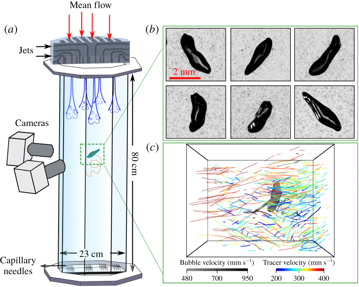
In this paper, as shown in figure 1, experiments were performed in the V-ONSET facility (Masuk et al. Reference Masuk, Salibindla, Tan and Ni2019b), a vertical water tunnel with an octagonal test section. The octagonal test section was designed to provide optical access to the centre of the tunnel through multiple flat surfaces (figure 1a). An array with 88 nozzles (5 mm in diameter) was fabricated using additive manufacturing and was utilized to inject high-speed water jets (up to $12~\text{m}~\text{s}^{-1}$) into the test section to drive turbulence. The resulting turbulence is close to being homogeneous and isotropic with a large energy dissipation rate $\unicode[STIX]{x1D716}\approx 0.5~\text{m}^{2}~\text{s}^{-3}$. The Kolmogorov length scale ($\unicode[STIX]{x1D702}$) and time scale ($\unicode[STIX]{x1D70F}_{\unicode[STIX]{x1D702}}$) of the system are $38~\unicode[STIX]{x03BC}\text{m}$ and 1.4 ms, respectively. Here $L$ is 3.2 cm and the fluctuation velocity $u^{\prime }=0.25~\text{m}~\text{s}^{-1}$. Finally, $Re_{\unicode[STIX]{x1D706}}$ is kept at around 346 in our system.

Figure 1.

(a) Schematic of the test section of V-ONSET (Masuk et al. Reference Masuk, Salibindla, Tan and Ni2019b). (b) Images of a deforming bubble with surrounding tracer particles on six cameras. (c) Sample of reconstructed three-dimensional tracer tracks around a bubble (Masuk, Salibindla & Ni Reference Masuk, Salibindla and Ni2019a). The instantaneous velocity magnitudes of both the bubble and surrounding tracers are colour-coded.

Air bubbles were injected into this system using capillary needles located at the bottom of the test section. Varying the needle size and airflow rates allows for the injection of bubbles of different sizes. These bubbles slowly rose up into the centre of the test section, where they interacted with the homogeneous isotropic turbulence generated by the jet array. In addition to the turbulence created by jets, a constant downward mean flow was employed to keep bubbles in the view area for an extended period of time. Furthermore, the carrier phase was seeded with $50~\unicode[STIX]{x03BC}\text{m}$ tracer particles that were used to quantify local flows around bubbles. The details of this facility and its flow characteristics can be found in Masuk et al. (Reference Masuk, Salibindla, Tan and Ni2019b).

The dynamics of bubbles and surrounding tracer particles were tracked by six high-speed cameras within a view volume of roughly $6\times 6\times 6~\text{cm}^{3}$. These cameras are capable of recording images at 4000 frames per second with one-megapixel resolution. Each camera had a dedicated light-emitting diode panel at the opposing side across the tunnel that cast shadows of bubbles and tracer particles onto the camera imaging plane. These images, as shown in figure 1(b), were then processed to separate the two phases. Six cameras were employed primarily for accurately reconstructing bubble shape. The collected images were processed by a virtual-camera visual hull method (Masuk et al. Reference Masuk, Salibindla and Ni2019a) to optimize the geometry by enforcing constraints imposed by the surface tension. After reconstruction, we tracked the centre of mass of roughly 29 000 bubbles (an example of such is shown in figure 1c). The trajectory of each bubble, on average, consists of 360 frames. In total, about $10^{7}$ data points of the local vertical bubble velocity $u_{z,b}$ were collected. Simultaneously, the mean volumetric flow rate of water through the tunnel was monitored by a digital flow meter, from which the mean vertical flow velocity $\overline{w}$, averaged over the entire cross-section, can be determined. Velocity $\overline{w}$ has to be subtracted from $u_{z,b}$ to obtain the bubble rise velocity: $w_{b}=u_{z,b}-\overline{w}$.

In addition, in each frame, over 6000 tracer particles were tracked simultaneously using our in-house high-concentration particle tracking code (Tan et al. Reference Tan, Salibindla, Masuk and Ni2019, Reference Tan, Salibindla, Masuk and Ni2020). A snapshot of our three-dimensional reconstructed results, including both three-dimensional bubble geometry and three-dimensional tracks of surrounding tracers, is shown in figure 1(c). Within a certain search radius ($\text{SR}=1.5D{-}3D$) from the centre of a bubble, $N$ tracer particles can be identified ($N$ ranges from 5 to 30 particles). Averaging the velocity of all these tracer particles $u_{z,i}$ helps to estimate the local flow velocity $u_{z,l}=\sum _{i=1}^{N}u_{z,i}/N$ at the centre of the bubble. In the governing equation ((4.1) in § 4) for bubbles (Magnaudet & Eames Reference Magnaudet and Eames2000), it is clearly stated that the fluid velocity used has to be the unperturbed ambient flow taken at the centre of a bubble if the bubble was not there. The local flow velocity $\overline{w_{s}}$, averaged across a small region where bubbles passed by, is found to be larger than $\overline{w}$ for the remaining regions because rising bubbles always drag surrounding fluid with them (Liu et al. Reference Liu, Zheng, Jia and Zhang2005; Lewandowski et al. Reference Lewandowski, Fertig, Krekel and Ulbricht2018; Risso Reference Risso2018). This perturbed flow $\overline{w_{s}}$ has to be subtracted from $u_{z,l}$ to estimate the unperturbed vertical flow velocity, i.e. $w_{l}=u_{z,l}-\overline{w_{s}}$.

4 Results and discussion

Figure 2.

Mean bubble rise velocity $\langle w_{b}\rangle$ as a function of bubble diameter $D$ in purified water (Clift, Grace & Weber Reference Clift, Grace and Weber2005) ($\times$); contaminated water (Clift et al. 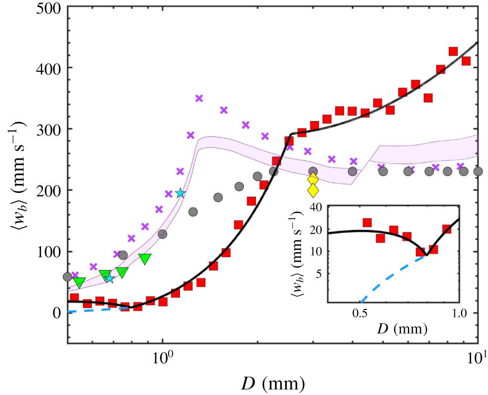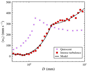Reference Clift, Grace and Weber2005) (●); weak turbulence ($We\ll 1<Eo$), including Aliseda & Lasheras (Reference Aliseda and Lasheras2011) (▼), Poorte & Biesheuvel (Reference Poorte and Biesheuvel2002) ($\star$) and Prakash et al. (Reference Prakash, Tagawa, Calzavarini, Mercado, Toschi, Lohse and Sun2012) (♦); and our experiments for intense turbulence (▪). Lines represent the model prediction for different conditions. The solid black line is calculated from our model, based on (4.3)–(4.5) at a high $\unicode[STIX]{x1D716}=0.5~\text{m}^{2}~\text{s}^{-3}$. The purple shaded area represents the model prediction for weak turbulence ($We\ll 1<Eo$) with $\unicode[STIX]{x1D716}=1.3\times 10^{-4}$–$6\times 10^{-3}~\text{m}^{2}~\text{s}^{-3}$ in clean water. The inset shows the same model prediction but using two lift models as shown in (4.8) and figure 3(b).

Figure 2 shows the ensemble average of bubble rise velocity $\langle w_{b}\rangle$ as a function of bubble size. Three groups of data, including bubbles rising in a quiescent medium (Clift et al. Reference Clift, Grace and Weber2005), weak turbulence ($We\ll Eo$, $\unicode[STIX]{x1D716}=1.3\times 10^{-4}$–$6\times 10^{-3}~\text{m}^{2}~\text{s}^{-3}$) (Poorte & Biesheuvel Reference Poorte and Biesheuvel2002; Aliseda & Lasheras Reference Aliseda and Lasheras2011; Prakash et al. Reference Prakash, Tagawa, Calzavarini, Mercado, Toschi, Lohse and Sun2012) and our experiments (strong turbulence, $\unicode[STIX]{x1D716}=0.5~\text{m}^{2}~\text{s}^{-3}$), are shown and compared to each other. For bubbles rising in a quiescent medium, $\langle w_{b}\rangle$ of small bubbles increases as $D$ grows because of buoyancy. For large bubbles, the pressure drag induced by flow separation and wake formation limit $\langle w_{b}\rangle$. When the background flow becomes weakly turbulent, $\langle w_{b}\rangle$ still maintains a trend similar to that observed for bubbles rising in an otherwise quiescent medium, but the magnitude is about 30–40 % smaller.

Once $\unicode[STIX]{x1D716}$ reaches $0.5~\text{m}^{2}~\text{s}^{-3}$ ($We$ becomes important), a clear deviation from both the quiescent and weakly turbulent cases is observed; not just the magnitude, but the entire dependence of $\langle w_{b}\rangle$ on the bubble size $D$ is altered. Three regimes are clearly observed: (i) $\langle w_{b}\rangle$ decreases by a factor of two as $D$ grows from 0.5 mm ($13.5\unicode[STIX]{x1D702}$) to 0.8 mm ($21.3\unicode[STIX]{x1D702}$), as shown in the inset of figure 2; (ii) $\langle w_{b}\rangle$ increases by over an order of magnitude for $D=0.8{-}2.2~\text{mm}$ ($21.3\unicode[STIX]{x1D702}{-}58.5\unicode[STIX]{x1D702}$); at 2.2 mm, $\langle w_{b}\rangle$ finally recovers the value in a quiescent medium; and (iii) for $D=2.2{-}10~\text{mm}$ ($58.5\unicode[STIX]{x1D702}{-}266\unicode[STIX]{x1D702}$), $\langle w_{b}\rangle$ continues to grow, exceeding the bubble rise velocity in a quiescent medium, although at a reduced growth rate. In sum, $\langle w_{b}\rangle$ varies from a factor of 11 (small bubbles) below that in a quiescent medium to almost two times above.

Figure 3.

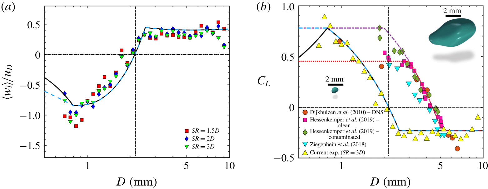
(a) The normalized mean vertical flow velocity $\langle w_{l}\rangle$ as a function of the bubble size $D$. Values of $\langle w_{l}\rangle$ are calculated based on three different SRs to find tracer particles around bubbles. (b) The lift coefficient $C_{L}$ as a function of bubble size. Yellow triangles represent results obtained from $\langle w_{l}\rangle$ and $\langle w_{b}\rangle$ based on (4.4). Other symbols represent results from laminar shear flows for air–water systems, which were fitted with a piece-wise linear function for purified water (dotted red line, equation (4.6)) and contaminated water (dash-dotted purple line, equation (4.7)). Cyan dashed line and black solid line (4.9) represent the revised lift models for intense turbulence. The vertical dashed lines in both panels mark the transition point where turbulence-based $We$ increases beyond 1. Two three-dimensional green blobs show the reconstructed three-dimensional shapes of small and large bubbles.

The observed change of $\langle w_{b}\rangle$ in intense turbulence must be a result of the coupling between bubbles and surrounding turbulent flows. To estimate the nearby flow velocity, similar to $\langle w_{b}\rangle$, $\langle w_{l}\rangle$ is determined by performing an ensemble average of $w_{l}$ over all bubbles of a particular size $D$. Figure 3(a) shows $\langle w_{l}\rangle$ as a function of the bubble size $D$. That $\langle w_{l}\rangle$ is negative for small bubbles clearly shows that the nearby flows around small bubbles, on average, move downward. Velocity $\langle w_{l}\rangle$ increases, crosses zero and finally becomes positive as $D$ grows, implying that the flows switch from hindering to assisting the rising motion of bubbles, which qualitatively explains why $\langle w_{b}\rangle$ exhibits such a dramatic change in figure 2. Different symbols in figure 3(a) correspond to different SRs used for selecting tracer particles around a bubble to estimate $w_{l}$. Note that very few particles can be triangulated within $1D$ away from the bubble centre as tracers close to a bubble can be easily shadowed by the bubble itself. Nevertheless, as flows in the close vicinity of a bubble ($\text{SR}<1D$) are heavily modulated by the bubble motion, excluding these tracers from the statistics could help to avoid statistical bias. From $\text{SR}=1.5D$ to $3D$, although with some variations, the observed trend of $\langle w_{l}\rangle$ seems to be consistent and insensitive to SR for bubbles with $D>1~\text{mm}$. As SR also affects the number of tracer particles included for calculating $\langle w_{l}\rangle$, this consistent trend also implies well-converged statistics for bubbles with $D>1~\text{mm}$. For small bubbles, results become sensitive to SR because of the insufficient number of tracers found within such a small SR.

Independent measurements of bubbles and surrounding tracers provide a consistent picture that bubbles of different sizes seem to be preferentially swept to regions with apparently opposing flow directions. The proposed mechanism of preferential sampling seems to be supported by the observed trend of $\langle w_{l}\rangle$. The surprising new finding is that bubbles do not always preferentially sample the downward flow side; the flow direction can be reversed for bubbles of large sizes. On the other hand, it may also imply that the vortex trapping idea does not apply to large bubbles, as vortex trapping is often linked to the pressure gradient force without considering the lift force. As a result, bubbles of all sizes would end up being trapped in the centre of eddies with an overall reduced rise velocity, which does not agree with our observation.

To understand the reason behind the reversal of the preferential sampling direction, we start from the governing equation for finite-sized bubbles (Magnaudet & Eames Reference Magnaudet and Eames2000):

(4.1)$$\begin{eqnarray}\displaystyle V_{b}(\unicode[STIX]{x1D70C}_{b}+C_{A}\unicode[STIX]{x1D70C}_{l})\frac{\text{D}\boldsymbol{u}_{\boldsymbol{b}}}{\text{D}t} & = & \displaystyle \unicode[STIX]{x1D70C}_{l}V_{b}C_{A}\frac{\text{D}\boldsymbol{u}_{\boldsymbol{l}}}{\text{D}t}+V_{b}(\unicode[STIX]{x1D70C}_{l}-\unicode[STIX]{x1D70C}_{b})g\hat{\boldsymbol{e}}_{z}+\frac{\unicode[STIX]{x1D70C}_{l}}{2}AC_{D}(\boldsymbol{u}_{l}-\boldsymbol{u}_{b})|\boldsymbol{u}_{l}-\boldsymbol{u}_{b}|\nonumber\\ \displaystyle & & \displaystyle +\,\unicode[STIX]{x1D70C}_{l}C_{L}(\boldsymbol{u}_{l}-\boldsymbol{u}_{b})\times (\unicode[STIX]{x1D735}\times \boldsymbol{u}_{\boldsymbol{l}})-\frac{1}{2}V_{b}\unicode[STIX]{x1D735}P_{w}+\boldsymbol{F}_{b},\end{eqnarray}$$

where $\unicode[STIX]{x1D70C}_{l}$ and $\unicode[STIX]{x1D70C}_{b}$ are the density of water and gas, respectively; $V_{b}$ is the bubble volume; $A$ is the projected area of a sphere with an equivalent volume of the bubble; $\boldsymbol{u}_{\boldsymbol{l}}$ is the velocity of the unperturbed ambient flow taken at the centre of the bubble; $\boldsymbol{F}_{b}$ is the Basset history force; and $C_{D}$, $C_{L}$ and $C_{A}$ are the drag coefficient, lift coefficient and added mass coefficient, respectively.

Taking an ensemble average of both sides of (4.1) yields

(4.2)$$\begin{eqnarray}0=V_{b}(\unicode[STIX]{x1D70C}_{l}-\unicode[STIX]{x1D70C}_{b})g\hat{\boldsymbol{e}}_{z}+\frac{\unicode[STIX]{x1D70C}_{l}}{2}AC_{D}\langle (\boldsymbol{u}_{l}-\boldsymbol{u}_{b})|\boldsymbol{u}_{l}-\boldsymbol{u}_{b}|\rangle +\unicode[STIX]{x1D70C}_{l}C_{L}\langle (\boldsymbol{u}_{l}-\boldsymbol{u}_{b})\times (\unicode[STIX]{x1D735}\times \boldsymbol{u}_{\boldsymbol{l}})\rangle -\frac{1}{2}V_{b}\langle \unicode[STIX]{x1D735}P_{w}\rangle\end{eqnarray}$$

as $\langle \text{D}\boldsymbol{u}_{l}/\text{D}t\rangle =0$ and $\langle D\boldsymbol{u}_{\boldsymbol{b}}/\text{D}t\rangle =0$ in homogeneous and isotropic turbulence, and the unsteady forces, including added mass and the Basset history force, become zero. In addition, the slip velocity between the two phases $\langle \boldsymbol{u}_{l}-\boldsymbol{u}_{b}\rangle$ is zero along the lateral directions and non-zero only along the vertical direction, which have been directly calculated from experiments and confirmed: $\langle \boldsymbol{u}_{l}-\boldsymbol{u}_{b}\rangle =\langle (w_{l}-w_{b})\rangle =\langle w_{l}\rangle -\langle w_{b}\rangle$. The same principle applies to $\langle (\boldsymbol{u}_{l}-\boldsymbol{u}_{b})|\boldsymbol{u}_{l}-\boldsymbol{u}_{b}|\rangle$, where only the vertical direction survives after the ensemble average: $\langle (\boldsymbol{u}_{l}-\boldsymbol{u}_{b})|\boldsymbol{u}_{l}-\boldsymbol{u}_{b}|\rangle \approx (\langle w_{b}\rangle -\langle w_{l}\rangle )^{2}$.

Figure 4.

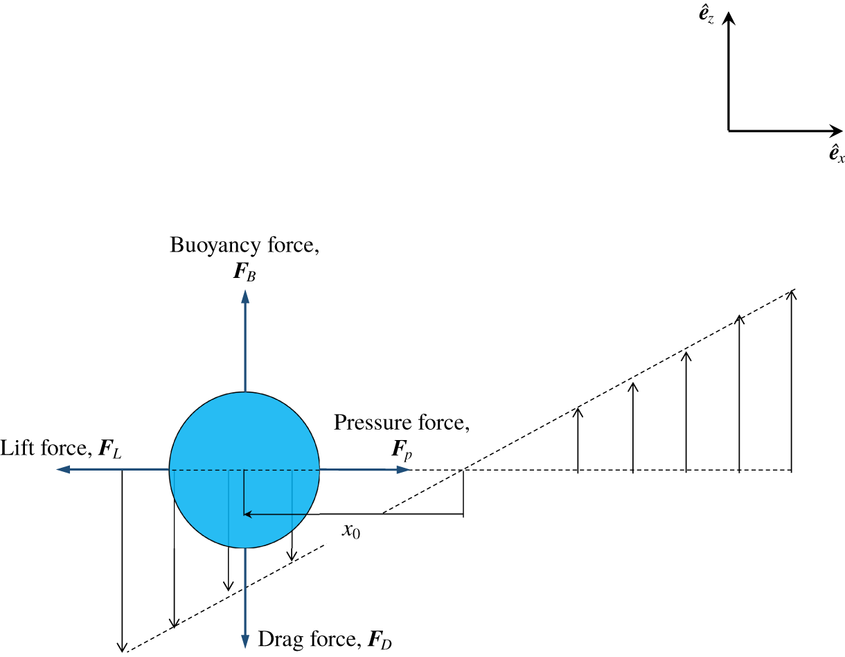
Schematic of a model for a bubble interacting with a uniform shear flow of constant shear rate ($\unicode[STIX]{x1D6FE}$) to represent the ensemble-averaged bubble–eddy interaction. Four forces experienced by the bubble in (4.2) must balance with each other along two orthogonal directions.

The remaining two terms, the lift force and the pressure force, are associated with $\langle \unicode[STIX]{x1D735}\times \boldsymbol{u}_{\boldsymbol{l}}\rangle$. We assume that the interaction between a bubble and its surrounding flows can be modelled as a bubble interacting with local shear with shear rate of $\unicode[STIX]{x1D6FE}=\langle \unicode[STIX]{x1D735}\times \boldsymbol{u}_{\boldsymbol{l}}\rangle =\text{d}\langle w_{l}\rangle /\text{d}x$, as depicted in figure 4. For the mean pressure force $\boldsymbol{F}_{p}=V_{b}\langle \unicode[STIX]{x1D735}P_{w}/2\rangle$, solving the Poisson equation for pressure yields $\unicode[STIX]{x1D735}P_{w}=\unicode[STIX]{x2202}P_{w}(x)/\unicode[STIX]{x2202}x=\unicode[STIX]{x1D70C}_{l}\unicode[STIX]{x1D6FE}^{2}x\hat{\boldsymbol{e}_{\boldsymbol{x}}}$. This indicates that the pressure force acts mainly along the horizontal direction $\hat{\boldsymbol{e}_{\boldsymbol{x}}}$. For the same configuration, the ensemble average of lift $\boldsymbol{F}_{L}=\unicode[STIX]{x1D70C}_{l}C_{L}(\boldsymbol{u}_{l}-\boldsymbol{u}_{b})\times (\unicode[STIX]{x1D735}\times \boldsymbol{u}_{\boldsymbol{l}})$ can be approximated as $\unicode[STIX]{x1D70C}_{l}C_{L}(\langle w_{l}\rangle -\langle w_{b}\rangle )|\unicode[STIX]{x1D6FE}|\hat{\boldsymbol{e}_{\boldsymbol{x}}}$. In figure 4, it may seem that we picked the flow orientation so that the direction of $\boldsymbol{F}_{L}$, i.e. $\hat{\boldsymbol{e}_{\boldsymbol{x}}}$, aligns with that of $\boldsymbol{F}_{\boldsymbol{p}}$. But this is not a coincidence. As shown in the vector equation (4.2), out of four terms, buoyancy and the ensemble-averaged drag are along the vertical direction, $\hat{\boldsymbol{e}_{\boldsymbol{z}}}$. The remaining two terms either have to share the same direction, or both of them have to be zero.

Following this argument, equation (4.2) can be written as two explicit equations along the vertical and lateral directions:

(4.3)$$\begin{eqnarray}\displaystyle & \displaystyle V_{b}(\unicode[STIX]{x1D70C}_{l}-\unicode[STIX]{x1D70C}_{b})g\hat{\boldsymbol{e}}_{z}={\textstyle \frac{1}{2}}AC_{D}(\langle w_{b}\rangle -\langle w_{l}\rangle )^{2}\hat{\boldsymbol{e}_{\boldsymbol{ z}}}, & \displaystyle\end{eqnarray}$$

(4.4)$$\begin{eqnarray}\displaystyle & \displaystyle \unicode[STIX]{x1D70C}_{l}C_{L}(\langle w_{l}\rangle -\langle w_{b}\rangle )|\unicode[STIX]{x1D6FE}|\hat{\boldsymbol{e}_{\boldsymbol{x}}}=\unicode[STIX]{x1D70C}_{l}\unicode[STIX]{x1D6FE}^{2}x_{0}\hat{\boldsymbol{e}_{\boldsymbol{x}}}, & \displaystyle\end{eqnarray}$$

where $x_{0}$ represents the steady lateral location of bubbles within the shear flow (figure 4). The mean flow velocity $\langle w_{l}\rangle$ at this location can be calculated:

(4.5)$$\begin{eqnarray}\langle w_{l}\rangle =\unicode[STIX]{x1D6FE}x_{0}.\end{eqnarray}$$

Positive or negative values of $x_{0}$ represent a bubble being swept to the upward or downward side of the shear, respectively. Shear rate $\unicode[STIX]{x1D6FE}$ scales with the velocity gradient of scale $D$, which can be related to the transverse second-order structure function $D_{NN}=4(\unicode[STIX]{x1D716}D)^{2/3}/3$ in the form of $\unicode[STIX]{x1D6FE}\sim 2(\sqrt{D_{NN}})/D=\sqrt{16/3}(\unicode[STIX]{x1D716}/D^{2})^{1/3}$. This is where $\unicode[STIX]{x1D716}$ enters the model.

Equations (4.3)–(4.5) provide a simple model for the ensemble-averaged fluid and bubble velocity, which can be measured directly from our experiments. There are three unknowns in these three equations: $C_{D}$, $C_{L}$ and $x_{0}$. This indicates that these three unknowns can be linked to the measured results exactly without any fitting parameters. Solving these linear equations is straightforward. For example, from (4.4), $x_{0}=C_{L}(\langle w_{l}\rangle -\langle w_{b}\rangle )/\unicode[STIX]{x1D6FE}$. As shown in figure 4, once $x_{0}$ is known based on (4.5), the flow velocity experienced by bubbles is simply the velocity at location $x_{0}$: $\langle w_{l}\rangle =\unicode[STIX]{x1D6FE}x_{0}=C_{L}(\langle w_{l}\rangle -\langle w_{b}\rangle )$.

This relationship suggests that $C_{L}$ can be directly obtained from our measurements of $\langle w_{l}\rangle$ and $\langle w_{b}\rangle$. The results are shown as yellow triangles in figure 3(b). Only one SR, i.e. $3D$, is used as $\langle w_{l}\rangle$ is not very sensitive to SR. For small bubbles ($D<2~\text{mm}$), $C_{L}$ is positive. As $D$ increases, $C_{L}$ continues to decrease until it reaches a negative value of $-0.23$. This transition indicates an inversion of the direction of this lateral lift.

Similar lift direction inversion has also been observed in different types of flows: bubbles rising in laminar shear flows (Tomiyama et al. Reference Tomiyama, Tamai, Zun and Hosokawa2002; Dijkhuizen, van Sint Annaland & Kuipers Reference Dijkhuizen, van Sint Annaland and Kuipers2010; Ziegenhein, Tomiyama & Lucas Reference Ziegenhein, Tomiyama and Lucas2018; Hessenkemper, Ziegenhein & Lucas Reference Hessenkemper, Ziegenhein and Lucas2019) and bubbles in channel flows (Lu & Tryggvason Reference Lu and Tryggvason2008, Reference Lu and Tryggvason2013; Dabiri, Lu & Tryggvason Reference Dabiri, Lu and Tryggvason2013). Although neither of these two cases is turbulent, the mean shear is large enough to allow for the lift force to drive bubbles in the lateral directions. It was shown that small spherical bubbles tend to migrate towards the low-speed side whereas large deforming bubbles favour the opposing high-speed side (Tomiyama et al. Reference Tomiyama, Tamai, Zun and Hosokawa2002) because of the interaction between shear and bubble deformation (Lu & Tryggvason Reference Lu and Tryggvason2008; Adoua, Legendre & Magnaudet Reference Adoua, Legendre and Magnaudet2009). Although no mean shear exists in our system – flow is close to homogeneous and isotropic (Masuk et al. Reference Masuk, Salibindla, Tan and Ni2019b) – deformable bubbles could respond to the local shear created by turbulent eddies.

To compare $C_{L}$ in the two systems more quantitatively, in figure 3(b), several recent datasets of $C_{L}$ for bubbles rising in laminar shear flows (limited to air–water systems) (Dijkhuizen et al. Reference Dijkhuizen, van Sint Annaland and Kuipers2010; Ziegenhein et al. Reference Ziegenhein, Tomiyama and Lucas2018; Hessenkemper et al. Reference Hessenkemper, Ziegenhein and Lucas2019) are also shown. All results are consistent – $C_{L}$ decays as $D$ grows and eventually it becomes negative, which marks the direction reversal of the bubble transverse migration driven by lift. The transition location of $C_{L}$ is believed to be associated with the buoyancy-induced deformation measured by $Eo$.

The inversion of $C_{L}$ seems to occur at a larger $D$ for the buoyancy-induced deformation than for the turbulence-driven cases. This difference can be attributed to different driving mechanisms of bubble deformation. In laminar shear flows, bubble deformation is only driven by buoyancy, measured by $Eo$. In our experiments, the lift inversion occurs when the bubble size increases from 2.2 mm ($We=0.71$) to 2.7 mm ($We=1.00$). As $We$ crosses from below to above one, turbulence-induced bubble deformation becomes important. Note that this $We$ does not account for bubble slip velocity or turbulence intermittency, which will only intensify the turbulence-induced deformation. Nevertheless, even without other compounding effects, this Weber number alone already indicates a possibility of an early lift inversion because of turbulence.

Other than the transition diameter, the trend of $C_{L}$ from our experiments is very similar to that from laminar shear flows, both of which can be fitted with piece-wise linear functions. For laminar shear flows, given the difference between contaminated water and purified water, two separate fits can be provided:

(4.6)$$\begin{eqnarray}\displaystyle & \displaystyle C_{L}=\left\{\begin{array}{@{}ll@{}}0.45\quad & Eo<1.25\text{ (pure water)},\\ 1.453-0.9\sqrt{Eo}\quad & 1.25<Eo<4,\\ -0.23\quad & 4<Eo,\end{array}\right. & \displaystyle\end{eqnarray}$$

(4.7)$$\begin{eqnarray}\displaystyle & \displaystyle C_{L}=\left\{\begin{array}{@{}ll@{}}0.78\quad & Eo<0.5\text{ (contaminated)},\\ 1.453-0.9\sqrt{Eo}\quad & 0.5<Eo<4,\\ -0.23\quad & 4<Eo.\end{array}\right. & \displaystyle\end{eqnarray}$$

In figure 3(b), equations (4.6) and (4.7) are shown as the red dotted line and purple dash-dotted line, respectively. The two equations are essentially the same; the only difference resides at the small-$Eo$ limit. Note that these two equations are different from the proposed more complicated correlations of Legendre & Magnaudet (Reference Legendre and Magnaudet1998), Tomiyama et al. (Reference Tomiyama, Tamai, Zun and Hosokawa2002), Hibiki & Ishii (Reference Hibiki and Ishii2007) and Dijkhuizen et al. (Reference Dijkhuizen, van Sint Annaland and Kuipers2010). But the piece-wise linear correlations provide equally good fits for the data.

When turbulence becomes important ($We\gtrsim Eo$), the lift equation is adjusted to use $We$ rather than $Eo$. Since many tracer particles are present in our system, bubble behaviours in our system should be similar to those in a contaminated case (equation (4.7)). Based on this argument, by adopting the same two limiting values of $C_{L}$ from (4.7), a new equation of $C_{L}$ for the turbulence-induced deformation is obtained:

(4.8)$$\begin{eqnarray}C_{L}=\left\{\begin{array}{@{}ll@{}}0.78~(2.671We^{3/5})\quad & We<0.1\\ 1.25-1.608We^{3/5}\quad & 0.1<We<0.9,\\ -0.23\quad & 0.9<We.\end{array}\right.\end{eqnarray}$$

The equation is shown as the cyan dashed line in figure 3(b). Equation (4.8) seems to agree with the data very well. Note that both (4.7) and (4.8) are piece-wise linear as a function of the bubble size $D$. Once $Eo$ and $We$ are used, the equations become dependent on $\sqrt{Eo}$ and $We^{3/5}$ simply because $Eo\sim D^{2}$ and $We\sim D^{5/3}$.

The agreement between (4.8) and data is not perfect for small bubbles ($D<1~\text{mm}$) because many bubbles do not have an adequate number of tracer particles within a small SR of $3D$ to calculate $\langle w_{l}\rangle$. Unfortunately, this range is crucial to constrain the behaviour of $C_{L}$ for small bubbles, regarding which the community has not reached a consensus. The value of $C_{L}$ could either be constant (Hibiki & Ishii Reference Hibiki and Ishii2007; Ziegenhein et al. Reference Ziegenhein, Tomiyama and Lucas2018) or decrease to zero (Tomiyama et al. Reference Tomiyama, Tamai, Zun and Hosokawa2002). Equation (4.8) lists two possibilities of $C_{L}$ for $We<0.1$. These are that $C_{L}$ either stays constant at 0.78 (cyan dashed line in figure 3b) or decreases from 0.78 to 0 linearly as $D$ decreases from 0.8 mm to zero: $2.671We^{3/5}$ (solid line). Both of these lines are also shown in figure 3(a).

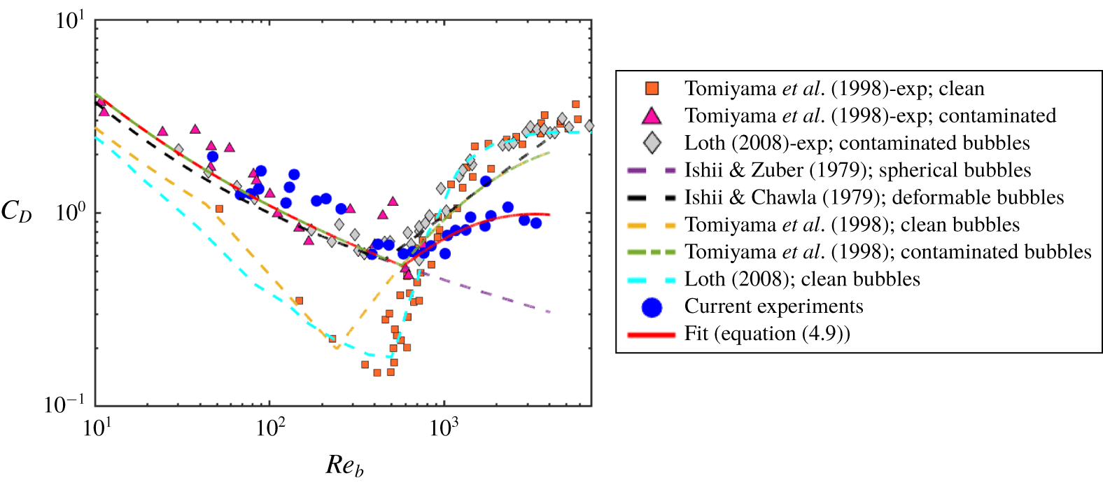
Once $C_{L}$ is known, the last unknown $C_{D}$ can be determined from (4.3). Figure 5 shows the calculated $C_{D}$ (blue circles) as a function of the bubble-scale Reynolds number, defined as $Re_{b}=(\langle w_{l}\rangle -\langle w_{b}\rangle )D/\unicode[STIX]{x1D708}$. For comparison, $C_{D}$ from other experiments (Ishii & Chawla Reference Ishii and Chawla1979; Ishii & Zuber Reference Ishii and Zuber1979; Tomiyama et al. Reference Tomiyama, Kataoka, Zun and Sakaguchi1998; Loth Reference Loth2008), including both clean and contaminated water, are also compiled in the same figure.

For small bubbles ($Re_{b}<400$), our results agree very well with the data of Tomiyama et al. (Reference Tomiyama, Kataoka, Zun and Sakaguchi1998) for bubbles rising in contaminated water (magenta triangles). As $Re_{b}$ exceeds 400, $C_{D}$ in intense turbulence becomes systematically lower. Since it occurs in the range of $Re_{b}$ where pressure drag induced by bubble wake also significantly increases $C_{D}$, it may imply that turbulence modulates the bubble wake dynamics. The eddy turnover time ($\unicode[STIX]{x1D70F}=\sqrt{4/3}(\unicode[STIX]{x1D716}^{-1/3}r^{2/3})=36.7~\text{ms}$ for $D=4~\text{mm}$) is much shorter than the wake shedding period based on the Strouhal number calculation ($\unicode[STIX]{x1D70F}_{w}=100~\text{ms}$ for $D=4~\text{mm}$) (Lindt Reference Lindt1972; Brücker Reference Brücker1999). This suggests that it is challenging for a bubble to develop an established wake as the incoming flow direction keeps varying. It may explain the smaller $C_{D}$ observed in intense turbulence compared to what has been found in a quiescent medium.

Figure 5.

The drag coefficient for bubbles versus the bubble-size-based Reynolds number $Re_{b}$. Data obtained from our experiments are shown as blue circles. The proposed corrected drag model is shown as the red solid line (equation (4.9)). Previous works on bubbles rising in clean and contaminated quiescent water as well as different models are shown as symbols and lines, respectively.

Here, we propose a corrected $C_{D}$ curve based on the turbulence-based Weber number. This revised drag coefficient model is

(4.9)$$\begin{eqnarray}C_{D}=\max (24/Re_{b}(1+0.15Re_{b}^{0.687}),\min (f(Eo),f(Eo)/We^{1/3})),\end{eqnarray}$$

where $f(Eo)=8Eo/3(Eo+4)$. Although the formulation seems long, it is essentially a combination of three equations for three regimes: (i) solid-sphere model $C_{D}=24/Re_{b}(1+0.15Re_{b}^{0.687})$ (Clift & Gauvin Reference Clift and Gauvin1971) for small bubbles with slightly contaminated interfaces, (ii) the phase velocity model $C_{D}=f(Eo)=8Eo/3(Eo+4)$ for large bubbles (Tomiyama et al. Reference Tomiyama, Kataoka, Zun and Sakaguchi1998) and (iii) our corrected model based on the Weber number $We$. For $We<1$, $C_{D}$ recovers the original formulation of $8Eo/3(Eo+4)$. For $We>1$, drag for large $Re_{b}$ is corrected to account for the modified wake effect. As shown in figure 5, this revised curve fits well to the measured results of $C_{D}$.

Based on (4.8) for $C_{L}$ and (4.9) for $C_{D}$, we can finally explain the surprising behaviour of $\langle w_{b}\rangle$ shown in figure 2. First of all, the overall trend of this curve is determined primarily by the direction inversion of the lateral lift. Intense turbulence with a large $\unicode[STIX]{x1D716}$ brings in two effects: (i) a strong local velocity gradient, which effectively increases the contribution of lift and pressure gradient, and (ii) enhanced eddy velocity. The first effect can markedly change the mean bubble rise velocity as bubbles are swept to different sides of eddies, and the second effect amplifies the magnitude change of $\langle w_{b}\rangle$. The behaviour of $\langle w_{b}\rangle$ for small bubbles ($D<1~\text{mm}$) is shown in the zoomed-in inset of figure 2. Two lines correspond to two different $C_{L}$ curves provided in (4.8). The solid line ($C_{L}=2.671We^{3/5}$ ($We<0.1$)) seems to agree better with $\langle w_{b}\rangle$.

Although our experiments were collected at a fixed $\unicode[STIX]{x1D716}$, we found three prior works (Poorte & Biesheuvel Reference Poorte and Biesheuvel2002; Aliseda & Lasheras Reference Aliseda and Lasheras2011; Prakash et al. Reference Prakash, Tagawa, Calzavarini, Mercado, Toschi, Lohse and Sun2012) involving different $\unicode[STIX]{x1D716}$ (ranging from $1.3\times 10^{-4}$ to $6\times 10^{-3}~\text{m}^{2}~\text{s}^{-3}$) that can also be used to test the model. For $\unicode[STIX]{x1D716}<0.1~\text{m}^{2}~\text{s}^{-3}$, $We$ is much smaller than $Eo$ for bubbles of size $D=0.5{-}3~\text{mm}$. Therefore, for these cases, bubble deformation is primarily driven by buoyancy, and the turbulence effect is secondary. Moreover, in weak turbulence, $We$ is not large enough to produce an early lift inversion. As a result, both $C_{L}$ and $C_{D}$ will recover that in a quiescent medium (red dotted line in figure 3(b) for $C_{L}$, and dashed green line in figure 5 for $C_{D}$). Taking both effects into consideration, the model prediction of $\langle w_{b}\rangle$ is shown in figure 2 as the purple shaded area (area covers the range of $\unicode[STIX]{x1D716}$ used in the three works), which passes through all the reported values. This area is indeed systematically lower than that for a quiescent medium by 20–40 %. This percentage change seems to be quite similar among these works despite a large range of $\unicode[STIX]{x1D716}$ used, which could be attributed to the saturation of $\langle w_{l}\rangle$. Since lift scales with $\unicode[STIX]{x1D6FE}$ and the pressure force scales with $\unicode[STIX]{x1D6FE}^{2}$, for small $\unicode[STIX]{x1D716}$, lift is always dominant, pushing bubbles to the edge of an eddy and saturating $\langle w_{l}\rangle$ at the maximum eddy velocity, ${\sim}\unicode[STIX]{x1D6FE}D/2$.

5 Summary

In summary, a new vertical water tunnel with a large energy dissipation rate was developed to study bubble dynamics in intense turbulence, in which turbulence-induced bubble deformation, measured by $We$, becomes close to or larger than buoyancy-induced deformation, quantified by $Eo$. Unlike other previous works conducted in weak turbulence ($Eo\gg We$), a surprising new behaviour of bubble rise velocity has been observed: within a small range of bubble sizes, bubble rise velocity transitions from an order of magnitude smaller to a factor of two larger than that in an otherwise quiescent medium.

Simultaneous measurements of dense tracer particles around bubbles show that flows around small bubbles move preferentially downward, hindering the rising motion of bubbles. Opposite upward flows are observed surrounding large bubbles, effectively increasing their rise velocity. This confirms the proposed preferential sampling mechanism that bubbles with different sizes tend to be swept to different regions in turbulence, rather than being trapped in the centre of eddies.

A model was derived by taking the ensemble average of both sides of the governing equation for bubble motion in turbulence. Since unsteady forces get averaged out in the process, only four forces, lift, buoyancy, drag and pressure gradient, are left in the equation. Two pairs of forces, buoyancy versus drag and lift versus pressure gradient, can be balanced along two orthogonal directions, which helps to utilize the measurable quantities, i.e. mean bubble and flow vertical velocity to estimate the drag and lift coefficients.

The lift coefficient shows clear direction inversion, similar to what has been extracted from experiments studying bubbles migrating in laminar shear flows. But in intense turbulence, $We\gtrsim Eo$, the transition occurs at a smaller bubble size when turbulence $We$ switches from below to above one. The drag coefficient is also modified for large bubbles. Strong turbulence potentially affects the formation of bubble wakes, which leads to a smaller drag coefficient. This effect also contributes to the enhanced rise velocity of bubbles. Finally, the model has also been tested on other datasets from previous works involving lower $\unicode[STIX]{x1D716}$; excellent agreement between the model predictions and the experimental results is observed without using any fitting parameters.